Phase transitions of quasistationary states in the Hamiltonian Mean Field model

Abstract

The out-of equilibrium dynamics of the Hamiltonian Mean Field (HMF) model is studied in presence of an externally imposed magnetic field $h$. Lynden-Bell’s theory of violent relaxation is revisited and shown to adequately capture the system dynamics, as revealed by direct Vlasov based numerical simulations in the limit of vanishing field. This includes the existence of an out-of-equilibrium phase transition separating magnetized and non magnetized phases. We also monitor the fluctuations in time of the magnetization, which allows us to elaborate on the choice of the correct order parameter when challenging the performance of Lynden-Bell’s theory. The presence of the field $h$ removes the phase transition, as it happens at equilibrium. Moreover, regions with negative susceptibility are numerically found to occur, in agreement with the predictions of the theory.

Long-range interacting systems are characterized by a slowly decaying interparticle potential, which in fact results in a substantial degree of coupling among far away components. In these systems, energy is consequently non-additive and this fact yields a large gallery of peculiar, apparently unintuitive, phenomena: the specific heat can be negative in the microcanonical ensemble, and temperature jumps may appear at microcanonical first-order phase transitions reviewRuffo ; Leshouches . Canonical and microcanonical statistical ensembles can therefore be non-equivalent in presence of long-range interactions, an intriguing possibility which has been thoroughly discussed working within simplified toy models.

Systems subject to long range couplings also display unexpected dynamical features. Starting from out-of-equilibrium initial conditions they are occasionally trapped in long lasting regimes, termed Quasi Stationary States (QSS), whose lifetime diverges with the number of elements, $N$, belonging to the system under scrutiny Yamaguchi .

The QSSs have been shown to relate to the stable steady states of the Vlasov equation, which governs the dynamical evolution of the single particle distribution function in the continuum limit $N\rightarrow\infty$ reviewRuffo ; Yamaguchi ; AntoniazziPRL1 ; fel . Working within this setting, one can implement an analytical procedure, fully justified from first principles, to clarify some aspects of QSS emergence. The idea, inspired to the seminal work of Lynden-Bell LyndenBell68 , is based on the definition of a locally-averaged (“coarse-grained”) distribution function, which translates into an entropy functional, as follows from standard statistical mechanics prescriptions. By maximizing such an entropy, while imposing the constraints of the dynamics, returns a closed analytical expression for the single particle distribution function of the system in its QSS regime. The predictive adequacy of the technique was tested versus numerical simulations for specific applications relevant in e.g. plasma physics, and for the Hamiltonian Mean Field (HMF) model antoni-95 , to which we will make extensive reference in the following. Furthermore, the Lynden-Bell approach allows one to successfully identify out-of-equilibrium phase transitions separating homogeneous and non homogeneous steady states Chavanis_phasetransition ; AntoniazziPRL2 . More recently, the Lynden-Bell procedure was applied to an open HMF system, modified by the inclusion of an externally imposed field, prognosticating the existence of regions of negative susceptibility which were then observed in direct simulations of the discrete Hamiltonian DeninnoFanelliEPL .

In this paper we revisit the Lynden-Bell analysis for the HMF model. The theoretical scenario is tested versus Vlasov based simulations, returning an overall good agreement. We discuss also the impact of the choice of a monitored quantity on the characterization of the order of the phase transition in absence of the external field. The role of the externally imposed field is assessed, with emphasis on the modification of the Lynden-Bell transition. The response of the system to the external forcing results in a smoothing of the transition that separates homogeneous and non homogeneous regimes, an observation which a posteriori supports the identification of such phenomenon with a genuine phase transition. We here anticipate that regions with negative susceptibility will be also identified in agreement with the Lynden-Bell scenario depicted in DeninnoFanelliEPL .

The paper is organized as follows. The next section is devoted to introducing the HMF model and to discussing its continuous analogue. In Section II we present the Lynden-Bell calculation, revisiting the results with reference to the unforced system. In Section III we present the results of the numerical simulations, based on a Vlasov code, aimed at verifying Lynden-Bell’s prediction of the presence of an out-of-equilibrium phase transition in the HMF model. The effect of applying an external magnetic field $h$ is discussed in Section IV. Finally, in Section V we sum up and conclude.

I The Hamiltonian Mean Field model

The Hamiltonian Mean-Field (HMF) model antoni-95 describes the motion of $N$ classical rotors coupled through a mean-field interaction. The system, in its standard formulation, can be straightforwardly modified to include an external perturbation that acts on the particles as a magnetic-like field Chavanis_h . The model is mathematically defined by the following Hamiltonian:

$$H=\frac{1}{2}\sum_{j=1}^{N}p_{j}^{2}+\frac{1}{2N}\sum_{i,j=1}^{N}\left[1-\cos(\theta_{j}-\theta_{i})\right]-h\sum_{j=1}^{N}\cos(\theta_{j}),$$ (1)

where $\theta_{j}$ represents the orientation of the $j$-th rotor and $p_{j}$ is its angular momentum. The scalar parameter $h$ measures the strength of the magnetic field. Hamiltonian (1) with $h=0$ has been widely studied in the past as a prototype model of long-range interacting systems. To monitor the dynamics of the systems, one often refers to the magnetization, a collective variable defined as

$${\mathbf{m}}=\frac{1}{N}\sum_{i=1}^{N}(\cos\theta_{i},\sin\theta_{i})=(m_{x},m_{y})~{}.$$ (2)

The modulus of ${\mathbf{m}}$, $m=\sqrt{m_{x}^{2}+m_{y}^{2}}$, measures the degree of bunching of the rotors along a given direction. The model can be also interpreted as describing $N$ particles moving on a circle. Within this interpretation, magnetized regimes signal the presence of a localized agglomeration of particles on the circle.

As previously reported in the literature Yamaguchi , starting from an out-of-equilibrium initial condition, the system gets trapped in long lasting QSSs, whose macroscopic characteristics differ significantly from those associated to the corresponding equilibrium configurations. QSSs develop for both $h=0$ and $h\neq 0$ settings. In the $N\to\infty$ limit, the system is indefinitely stuck in the QSS phase.

On the other hand, when performing the limit for infinite system size, the discrete model Hamiltonian (1) admits a rigorous continuous analogue. This is the Vlasov equation which governs the evolution of the single particle distribution function $f(\theta,p,t)$:

$$\frac{\partial f}{\partial t} + p\,\frac{\partial f}{\partial\theta}-\frac{dV[f]}{d\theta}\frac{\partial f}{\partial p}=0\;,$$ (3)

$$V[f](\theta) = 1-\left(m_{x}[f]+h\right)\cos\theta-m_{y}[f]\sin\theta\;,$$ (5)

$$m_{x}[f] = \int d\theta\,dp\,f\cos\theta\;,$$ (6)

$$m_{y}[f] = \int d\theta\,dp\,f\sin\theta\;,$$ (7)

where $V$ is the interaction potential that depends self-consistently on $f(\theta,p,t)$. According to this kinetic picture the free streaming of the particles is opposed by a potential term $V[f]$, reminiscent of the discrete formulation, expressed as a self-consistent function of the dynamically varying distribution $f(\theta,p,t)$.

In light of the above, the QSSs have been interpreted as stable steady states of the underlying Vlasov equation. Working within this setting, and invoking the aforementioned Lynden–Bell violent relaxation theory LyndenBell68 , one can progress analytically at least for a simplified choice of the initial condition. A short account of the technicalities is provided in the following section.

II The maximum entropy solution

Assume the particles to be confined within a bounded domain of phase space, therein displaying a uniform probability distribution. Label $f_{0}$ the constant value of $f(\theta,p,t)$ within the selected domain, as imposed by the normalization condition. This working ansatz corresponds to dealing with the “waterbag” distribution:

$$f(\theta,p,0)=\left\{\begin{array}[]{ll}f_{0}=\frac{1}{4\Delta\theta\Delta p}&\textrm{if }-\Delta p<p<\Delta p\\ &\textrm{and }-\Delta\theta<\theta<\Delta\theta\\ 0&\textrm{otherwise,}\\ \end{array}\right.$$ (8)

that is even in both $\theta$ and $p$: $f(-\theta,-p,0)=f(\theta,p,0)$. For distributions endowed with this symmetry, it can be straightforwardly proven that, being $m_{y}=0$ initially, its value remains zero during time evolution. This in turn implies that also the total momentum $P=\int pf(\theta,p,t)d\theta dp$, which is zero initially, remains zero during the whole time evolution, i.e. there is no global rotation of the particles on the circle. With this choice, one parametrizes the initial condition in terms of the energy density $u=H/N$ and the initial magnetization ${\mathbf{m}}=(m_{0},0)$. Momentum $P$ cannot be considered as a global invariant, because the presence of an external magnetic field breaks the translation symmetry $\theta\to\theta+\alpha$. However, for the initial distributions (8), momentum is fixed to zero.

Under the Vlasov evolution, the waterbag gets distorted and filamented at smaller scales, while preserving its surface in phase space. The distribution stays two-level ($0,f_{0}$) as time progresses. By performing a local average of $f$ inside a given mesoscopic box, one gets a coarse-grained profile which is hereafter labelled $\bar{f}$. As opposed to $f$, the locally averaged function $\bar{f}$ converges to an asymptotic equilibrium solution which can be explicitly evaluated via a rigorous statistical mechanics procedure, adapted from the pioneering analysis of Lynden-Bell. An entropy functional $s(\bar{f})$, can be in fact associated to $\bar{f}$, through a direct combinatorial calculation LyndenBell68 . In the two-level waterbag scenario, the mixing entropy density $s$ takes the form:

$$s[\bar{f}]=-\int\!\!{\mathrm{d}}p{\mathrm{d}}\theta\,\left[\frac{\bar{f}}{f_{0}}\ln\frac{\bar{f}}{f_{0}}+\left(1-\frac{\bar{f}}{f_{0}}\right)\ln\left(1-\frac{\bar{f}}{f_{0}}\right)\right].$$ (9)

The energy density

$$u[\bar{f}]=\iint{\mathrm{d}}\theta{\mathrm{d}}p\frac{p^{2}}{2}f(\theta,p,t)+\frac{1-m_{x}^{2}-m_{y}^{2}}{2}-hm_{x}$$ (10)

is conserved. In addition, the normalization of the distribution $\bar{f}$ has to be imposed, which physically corresponds to assume constant mass. Requiring the entropy to be stationary, while imposing the conservation of energy and mass, result in a variational problem that admits the following solution:

$$\bar{f}_{\text{QSS}}(\theta,p)=\\ \frac{f_{0}}{1+e^{\displaystyle\beta f_{0}(p^{2}/2-{m}_{x}\cos\theta-{m}_{y}\sin\theta-h\cos\theta)+\alpha}},$$ (11)

where $\alpha$ and $\beta$ are Lagrange multipliers associated, respectively, to mass and energy conservation and $m_{x}$ and $m_{y}$ depend on $\bar{f}_{\text{QSS}}$. The self-consistent nature of Eq. (11) is evident: $m_{x}[\bar{f}_{\text{QSS}}]$ and $m_{y}[\bar{f}_{\text{QSS}}]$ are functionals of $\bar{f}_{\text{QSS}}$ and both enter in the determination of $\bar{f}_{\text{QSS}}$ itself. We also emphasize that the label QSS is introduced to recall that the stationary solution of the Vlasov equation are indeed associated to QSSs of the discrete $N$-body dynamics.

Back to solution (11), one can determine the predicted values of $m_{x}$, $m_{y}$, $\alpha$ and $\beta$ once the energy $e$, the field $h$ and the waterbag height $f_{0}$ are being assigned. This step is performed numerically, at sought accuracy, via a Newton-Raphson method.

Consider first the limiting case $h=0$. Depending on the value of the predicted magnetization $m$, one can ideally identify two different regimes: the homogeneous case corresponds to $m=0$ (non-magnetized), while the non-homogeneous setting is found for (magnetized) $m\neq 0$ solutions. A phase transition Chavanis_phasetransition ; AntoniazziPRL1 materializes in the parameters plane $(m_{0},u)$ and the resulting scenario is depicted in Fig. 1. When fixing the initial magnetization and decreasing the energy density, the system passes from homogeneous to non-homogeneous QSS. The parameters plane can be then formally partitioned into two zones respectively associated to an ordered non-homogeneous phase, $m\neq 0$, (lower part of Fig. 1), and a disordered homogeneous state, $m=0$ (upper part). These regions are delimited by a transition line, collection of all the critical points ($m_{0}^{c},u^{c}$), which can be in turn segmented into two distinct parts.

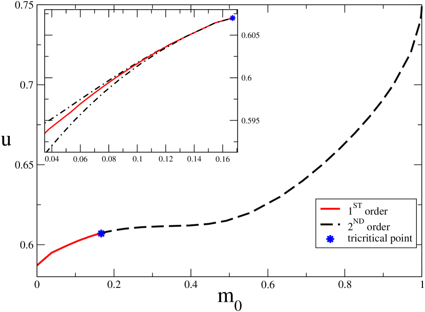
Figure 1: Phase diagram in the $(m_{0},u)$ plane at $h=0$. The full line refers to the the first order transition, while the dashed line stands for the second order one. The symbol traces the exact location of the tricritical point. Inset: lateral edges of the coexistence regions in the first order region, as predicted by the theory.

The full line stands for a first order phase transition: the magnetization experiences a finite jump when crossing the critical value ($m_{0}^{c},u^{c}$). Conversely, the dashed line refers to a second order phase transition: the magnetization is continuously modulated, from zero to positive values, when passing the curve from top to bottom. First and second lines merge in a tricritical point.

The case with $h\neq 0$ has been recently addressed in DeninnoFanelliEPL for what concerns the Lynden-Bell theory and working at constant $f_{0}$, while the equilibrium properties have been thoroughly studied in Chavanis_h . Again, the Lynden Bell approach proves accurate in predicting the macroscopic behavior as seen in the $N$-body simulations. Interestingly, below a threshold in energy the system shows negative susceptibility $\chi=\partial M/\partial h$, the magnetization decreasing when the strength of $h$ is enhanced. Conversely, above the critical energy value, the magnetization amount grows with $h$, which corresponds to dealing with positive susceptibility. Besides providing an a posteriori evidence on the adequacy of the Lynden-Bell technique, the presence of a region with negative susceptibility, was interpreted in DeninnoFanelliEPL as the signature of an out-of-equilibrium ensemble inequivalence. Furthermore, the presence of the field $h$ removes the phase transition and the magnetization continuously decreases from unity, at zero temperature, to zero, at infinite temperature. Therefore, a modest, though non negligible spatial polarization of the rotors is present also in the parameters region that was destined to homogeneous phases in the limiting case $h=0$.

Starting from this setting, we have decided to perform a campaign of Vlasov based simulations to challenge the rich scenario predicted within the realm of the Lynden-Bell violent relaxation theory. By numerically solving the Vlasov equation, we avoid dealing with finite size effects, as stemming in direct $N$-body schemes, and so provide a more reliable assessment of the overall correctness of the theory. The results of the investigations are reported in the forthcoming sections.

III Magnetization and its fluctuations

The Vlasov equation (3) can be resolved numerically. To this end, we use the semi-Lagrangian method with cubic spline interpolation, as implemented in the vmf90 program that has been used already in Ref. de_buyl_cnsns_2010 with the HMF model.

In order to study the properties of the QSS regime, we adopt the following procedure:

1. The system is started with a waterbag initial condition (8).

2. It is run without collecting data between times $t_{0}=0$ and $t_{1}=100$.

3. Time averages of the magnetization $m$, of $m_{x}$ and of the variance of the magnetization $m$ are performed in the time range between $t_{1}=100$ and $t_{2}=200$, defining

   $$\overline{m}=\frac{1}{t_{2}-t_{1}}\int_{t_{1}}^{t_{2}}m(t)dt~{},$$ (12)

   $$\overline{m}_{x}=\frac{1}{t_{2}-t_{1}}\int_{t_{1}}^{t_{2}}m_{x}(t)dt~{},$$ (13)

   $$\sigma_{m}^{2}=\frac{1}{t_{2}-t_{1}}\int_{t_{1}}^{t_{2}}(m(t)-\overline{m})^{2}dt~{}.$$ (14)

We thus skip the strong oscillations of the initial violent relaxation and focus on the subsequent dynamical regime, where, anyway, some oscillations are still present, which we quantify by the standard deviation $\sigma_{m}$. We repeat the above procedure on a grid of 39 by 39 points in the $(m_{0},u)$ plane, each one corresponding to a simulation. Performing such a study allows us to assess in a systematic manner the behaviour of the average magnetization in the QSS regime and to compare numerical results with Lynden-Bell’s theory. Whether the theory is flexible enough to accommodate all the general features of the resulting diagram depends on it taking into account in a comprehensive manner the behaviour of the model.

The average value of the magnetization taken from Vlasov simulations is displayed in Fig. 2. The line of transition provided by Lynden-Bell’s theory is displayed on top and we observe that it separates satisfactorily the region $m>0$ from the region $m\approx 0$ for $m_{0}\lesssim 0.6$. The transition is sharp for low values of $m_{0}$, corresponding to the prediction of Lynden-Bell’s theory that the transition is of first order. The transition is smoother for larger values of $m_{0}$, corresponding to the Lynden-Bell’s prediction of a second order transition.

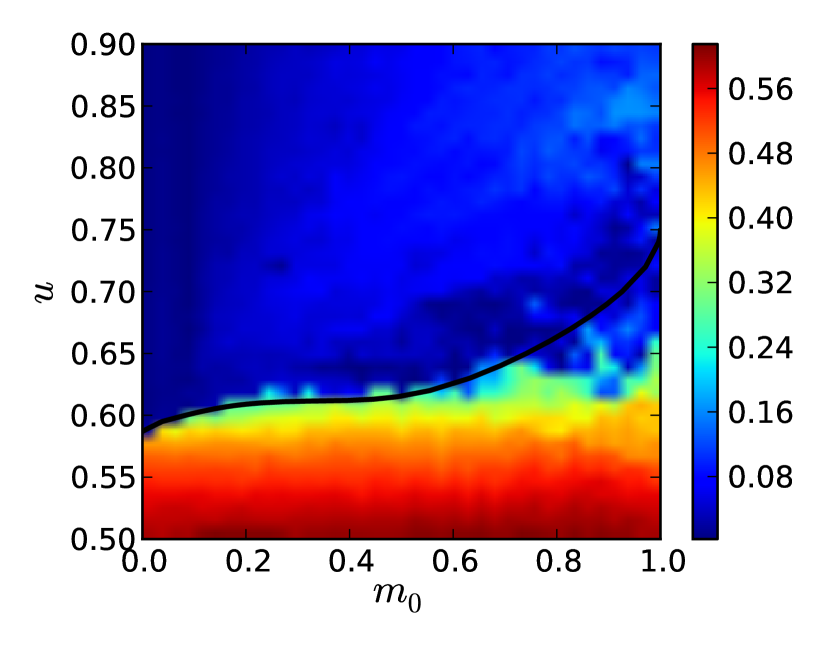
Figure 2: Average magnetization $\bar{m}$ for the HMF model with no external field. The transition predicted by Lynden-Bell’s theory is indicated by the full black line.

We display in Fig. 3 the same diagram as the one of Fig. 2, but using $\overline{m}_{x}$ instead of $\overline{m}$. The general aspect of the diagram is similar, although, as remarked in pakter_levin_prl_2011 , the transition looks overall sharper when using $\overline{m}_{x}$ as an order parameter. We note that Lynden-Bell’s transition line separates very well the non-homogeneous from the homogeneous phase for $m_{0}\lesssim 0.4$. For higher values of $m_{0}$ there are simulations for which $\overline{m}_{x}<0$ (blue spots below the Lynden-Bell’s transition line in Fig. 3). This occurs when the phase of ${\mathbf{m}}$ is $\pi$ (instead of zero). The phase could in principle take any value in $[-\pi,\pi]$, but since $m_{y}=0$ the only dynamically accessible values are $0$ and $\pi$. The fact that $m_{x}$ can flip from positive to negative values is also an indication of the presence of a second-order phase transition. Indeed, these flips are not present in the first order phase transition region, where an entropic barrier at the phase transition separates positive and negative values of $m_{x}$.

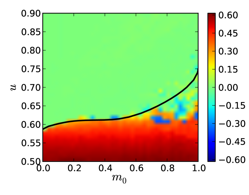
Figure 3: Average of the $x$-component of the magnetization $\overline{m}_{x}$ for the HMF model with no external field. The transition predicted by Lynden-Bell’s theory is indicated by the full black line.

The difference in the values of $\overline{m}$ and $\overline{m}_{x}$ can only arise from time fluctuations of $m_{x}(t)$. Indeed

$$\overline{m^{2}}=\overline{m_{x}^{2}}=\overline{m_{x}}^{2}+\sigma_{m}^{2}$$ (15)

To illustrate the difference between these two quantities, we compare them in Fig. 4 for $m_{0}=0.1$ and $0.4$.

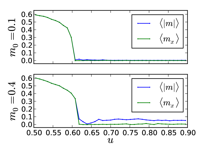
Figure 4: Comparison of $\overline{m}$ and $\overline{m}_{x}$ as a function of $u$ for $m_{0}=0.1$ and $m_{0}=0.4$.

In the low energy phase the two quantities are indistinguishable, prooving that the fluctuations are small. It is confirmed that $\overline{m}_{x}$ goes sharply to zero at the transitions energy and remains zero in the whole high energy phase, as found in pakter_levin_prl_2011 . On the contrary, $\overline{m}$, the quantity measured in AntoniazziPRL2 , has a tail of positive values at high energy, especially visible for $m_{0}=0.4$, proving that fluctuations are here larger.

The variance of the magnetization, $\sigma_{m}$, is displayed in Fig. 5. It is confirmed that, below the transition line predicted by Lynden-Bell’s theory, fluctuations of $m$ are small. They are instead large in the high energy region above the Lynden-Bell’s transition line for $m_{0}>0.4$.

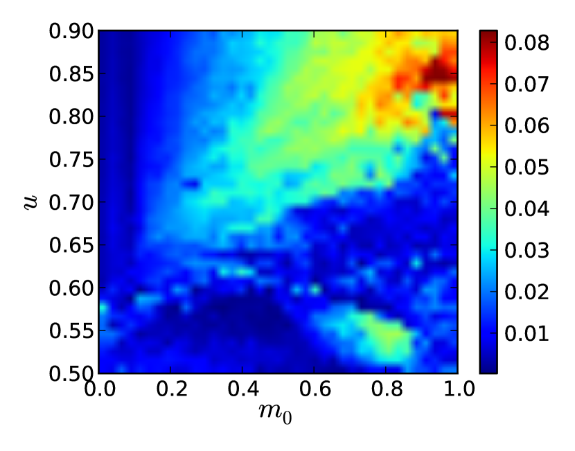
Figure 5: Amplitude of oscillations measured by $\sigma_{m}$ for the HMF model with no external field.

By pointing out the different results that arise from the choice of different order parameters, $\overline{m}$ or $\overline{m}_{x}$, we hope that in future studies the problem of the out-of-equilibrium phase transition in the HMF model will be analyzed more carefully.

IV Response to the application of a small magnetic field

In this Section, we present the results of simulations for the HMF model with a small external magnetic field, we choose $h=0.1$. The average value of the magnetization $\overline{m}$ obtained from Vlasov simulations is displayed in Fig. 6.

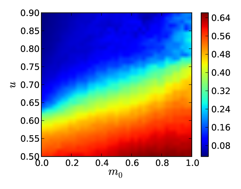
Figure 6: Average magnetization $\overline{m}$ for the HMF model with an external field $h=0.1$.

The phase transition is removed by the application of the field, as it happens for equilibrium phase transitions. The magnetization, for all values of $m_{0}$, decreases smoothly to zero as the energy is increased.

Magnetic susceptibility $\chi=\partial m/\partial h$ characterizes the response of the system to the application of an external field. It has been shown in Ref. DeninnoFanelliEPL that certain parameter regions display a negative magnetic susceptibility. This is a signature of ensemble inequivalence, shown here in a out-of-equilibrium setting, as the system is trapped in the QSS regime and does not reach equilibrium. In this Section, we provide a similar measure by taking the difference of the average magnetization between simulations with $h=0.1$ and simulations with $h=0$. The result is displayed in Fig. 7.

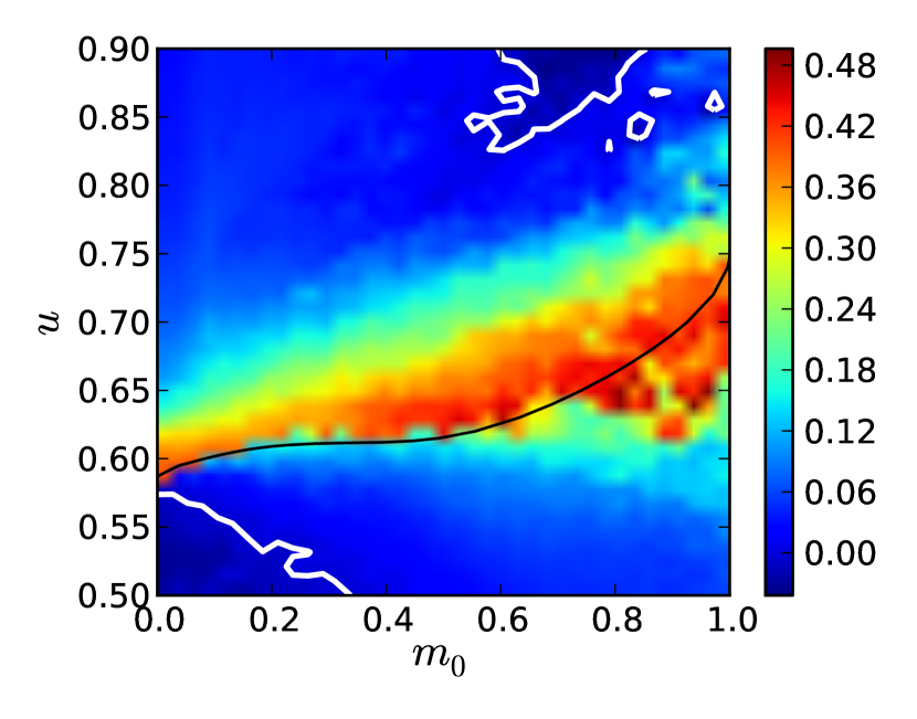
Figure 7: Difference of average magnetization between simulations with $h=0.1$ and simulations with $h=0$. The white lines indicate the zero level, so that the darker region close to ($m_{0}=0$,$u=1/2$) is a region of negative magnetic susceptibility.

While our computations provide a discrete difference instead of a derivative, obtaining a lower value of the average magnetization for $h=0.1$ than for $h=0$ is the sign of a negative susceptibility nonetheless. As expected from Ref. DeninnoFanelliEPL , a region of Fig. 7 displays $\chi<0$ for low values of $m_{0}$, in the vicinity of the first-order transition found in the theory. We are thus able to confirm the theoretical prediction on the basis of Vlasov simulations. Figure 7 also displays a large value of $\chi$ around the transition line predicted by Lynden-Bell’s theory.

V Conclusions

We have performed a study on the adequateness of Lynden-Bell’s theory as compared to numerical simulations of the Vlasov equation for the Hamiltonian Mean-Field model. Our results confirm previous studies based on $N$-body simulations on the general quality of the phase diagram. We extended the knowledge of the phase diagram by several additional measurements: the amplitude of oscillations, $\sigma_{m}$, the magnetic susceptibility. By doing so, we point out that in regions where non negligible fluctuations of the magnetization $m$ occur, the theory is not expected to work, whereas the agreement is quite good between numerical simulations and theory in regions where fluctuations are small. We also confirmed that there are regions of negative susceptibility, as predicted in Ref. DeninnoFanelliEPL .

Finally, we also discuss the more fundamental, but related issue, of the appropriate thermodynamical quantity to follow in the simulations. This latter issue is not touched upon in the literature but reveals qualitatively different results for the transition from magnetized to non-magnetized regimes. As of now, Lynden-Bell’s theory provides a clear determination of the order of the transition and a tricritical point is found in the phase diagram. However, the dynamical aspects of the transitions are not yet elucidated, as is known from numerical simulations, even if steps are taken in that direction pakter_levin_prl_2011 ; de_buyl_et_al_rsta_2011 ; de_buyl_et_al_in_prep .

VI Acknowledgements

D.F. thanks Giovanni De Ninno for discussions. S. R. acknowledges support of the contract LORIS (ANR-10-CEXC-010-01).

References

- (1) A. Campa, T. Dauxois and S. Ruffo, Phys. Rep. 480, 57 (2009).
- (2) T. Dauxois, S. Ruffo and L. Cugliandolo (Eds.), Long-Range Interacting Systems, Lecture Notes of the Les Houches Summer School: Volume 90, August 2008, Oxford University Press (2009).
- (3) Y.Y. Yamaguchi, J. Barré, F. Bouchet, T. Dauxois and S. Ruffo, Physica A 337, 36 (2004).
- (4) A. Antoniazzi, F. Califano, D. Fanelli and S. Ruffo, Phys. Rev. Lett. 98, 150602 (2007).
- (5) J. Barré, T. Dauxois, G. De Ninno, D. Fanelli and S. Ruffo, Phys. Rev. E 69, 045501(R) (2004).
- (6) D. Lynden-Bell and R. Wood, Mon. Not. R. Astron. Soc. 138, 495 (1968).
- (7) M. Antoni and S. Ruffo, Phys. Rev. E 52, 2361-2374 (1995).
- (8) P. H. Chavanis, Eur. Phys. J. B 53, 487 (2006).
- (9) A. Antoniazzi, D. Fanelli, S. Ruffo, Y.Y. Yamaguchi, Phys. Rev. Lett. 99, 040601 (2007).
- (10) G. De Ninno and D. Fanelli, Europhys. Lett. in press arXiv:1011.2981 (2011).
- (11) P. H. Chavanis, Eur. Phys. J. B 80, 275 (2011).
- (12) P. de Buyl,Commun. Nonlinear Sci. Numer. Simulat. 15, 2133-2139 (2010).
- (13) R. Pakter and Y. Levin, Phys. Rev. Lett. 106, 200603 (2011).
- (14) P. de Buyl, D. Mukamel and S. Ruffo, Phil. Trans. R. Soc. A, 369, 439 (2011).
- (15) P. de Buyl, D. Mukamel and S. Ruffo, arXiv:1012.2594 (2010).