Linear response theory for long-range interacting systems in quasistationary states

Abstract

Long-range interacting systems, while relaxing to equilibrium, often get trapped in long-lived quasistationary states which have lifetimes that diverge with the system size. In this work, we address the question of how a long-range system in a quasistationary state (QSS) responds to an external perturbation. We consider a long-range system that evolves under deterministic Hamiltonian dynamics. The perturbation is taken to couple to the canonical coordinates of the individual constituents. Our study is based on analyzing the Vlasov equation for the single-particle phase-space distribution. The QSS represents a stable stationary solution of the Vlasov equation in the absence of the external perturbation. In the presence of small perturbation, we linearize the perturbed Vlasov equation about the QSS to obtain a formal expression for the response observed in a single-particle dynamical quantity. For a QSS that is homogeneous in the coordinate, we obtain an explicit formula for the response. We apply our analysis to a paradigmatic model, the Hamiltonian mean-field model, which involves particles moving on a circle under Hamiltonian dynamics. Our prediction for the response of three representative QSSs in this model (the water-bag QSS, the Fermi-Dirac QSS, and the Gaussian QSS) is found to be in good agreement with $N$-particle simulations for large $N$. We also show the long-time relaxation of the water-bag QSS to the Boltzmann-Gibbs equilibrium state.

I Introduction

Systems with long-range interactions are ubiquitous in nature review3 ; review4 ; review5 . In these systems, the interaction potential between two particles decays asymptotically with separation $r$ as $1/r^{\alpha}$, where $\alpha$ is smaller than or equal to the spatial dimension of the system. Examples are dipolar ferroelectrics and ferromagnets, self-gravitating systems, non-neutral plasmas, two-dimensional geophysical vortices, etc. Long-range interactions result in non-additivity, thereby giving rise to equilibrium properties which are unusual for short-range systems, e.g., a negative microcanonical specific heat, inequivalence of statistical ensembles, and others review3 .

Long-range systems often exhibit intriguingly slow relaxation toward equilibrium Yamaguchi:2004 ; Joyce:2010 ; Levin:2010 ; Gupta:2011 . Such slow relaxation has been widely investigated in a model of globally coupled particles moving on a unit circle and evolving under Hamiltonian dynamics. This model is known as the Hamiltonian mean-field (HMF) model Ruffo:1995 . In this model, a wide class of initial conditions relaxes to equilibrium over times that diverge with the system size. It has been demonstrated that, depending on the initial condition, the relaxation to equilibrium for some energy interval occurs through intermediate long-lived quasistationary states (QSSs). These non-Boltzmann states involve slow evolution of thermodynamic observables over time, and have a lifetime which grows algebraically with the system size Yamaguchi:2004 . An immediate consequence is that the system, in the limit of infinite size, never attains the Boltzmann-Gibbs equilibrium, but remains trapped in the QSSs. Generalizations of the HMF model to include anisotropy terms in the energy Jain:2007 , and to particles which are confined to move on a spherical surface rather than on a circle Nobre:2003 have also shown slow relaxation toward equilibrium and the presence of QSSs.

Dynamics of systems with long-range interaction, in the infinite-size limit, is described by the Vlasov equation that governs the time evolution of the single-particle phase-space distribution Nicholson:1992 . This equation allows a wide class of stationary solutions. Their stability can be determined from the temporal behavior of small fluctuations by linearizing the Vlasov equation around the stationary solutions. Stable stationary states of the Vlasov equation correspond to QSSs of the finite-size system. The first clear demonstration of this correspondence was achieved for the HMF model Yamaguchi:2004 . In this paper, we refer interchangeably to stable stationary states of the Vlasov equation and QSSs of the finite-size dynamics.

The study of the time evolution of fluctuations around a stationary solution of the Vlasov dynamics is relevant in many applications, for instance, in the phenomenon of Landau damping that arises due to energy exchange between particles and waves in an electrostatic plasma Landau:1946 . In this process and in many others, spontaneous statistical fluctuations around a stable stationary state of the Vlasov equation are considered, and their rate of exponential decay in time is determined by solving an initial value problem involving the linearized Vlasov equation through a careful use of the Laplace-Fourier transform.

In this paper, we follow a different approach to the study of fluctuations by the linearized Vlasov equation. Inspired by Kubo linear response theory KuboJPSJ:1957 , we analyze the response of a Vlasov-stable stationary state to the application of a small external perturbation described by a time-dependent term in the Hamiltonian. The perturbation induces forced fluctuations around the stationary state that we treat to linear order in the strength of the perturbation, and study their evolution in time by using the linearized Vlasov equation. Such forced fluctuations are known to be generically finite for Boltzmann-Gibbs equilibrium states. We show here theoretically that they are finite and small, of the order of the perturbation, also for Vlasov-stable stationary states. We support our analysis with $N$-particle numerical simulations of the HMF model.

The paper is organized as follows. In Sec. II, we develop the linear response theory for a general QSS by using the Vlasov framework. In Sec. III, we specialize to a QSS that is homogeneous in the coordinate, and derive a closed form expression for the change induced by the external perturbation in a single-particle dynamical quantity. Section IV is devoted to the application of the theory to study the response of three representative homogeneous QSSs in the HMF model, namely, the widely studied water-bag QSS, the Fermi-Dirac QSS and the homogeneous equilibrium state, which is also a QSS. In the following section, we compare results from $N$-particle numerical simulations of the HMF dynamics with those from the linear response theory, and obtain good agreement. We also discuss the long-time relaxation of the water-bag QSS to Boltzmann-Gibbs equilibrium under the action of the perturbation. We draw our conclusions in Sec. VI.

II Linear response theory for QSS

Consider a system of $N$ particles interacting through a long-ranged pair potential. The Hamiltonian of the system is

$$H_{0}=\sum_{i=1}^{N}\frac{p_{i}^{2}}{2}+\frac{1}{N}\sum_{i<j}^{N}v(q_{i}-q_{j}),$$ (1)

where $q_{i}$ and $p_{i}$ are, respectively, the canonical coordinate and momentum of the $i$th particle, while $v(q_{i}-q_{j})$ is the interaction potential between the $i$th and $j$th particles. We assume that $v(q)$ is suitably regularized for zero argument. We regard $q_{i}$’s and $p_{i}$’s as one-dimensional variables, though our formalism may be easily extended to higher dimensions. The mass of the particles is taken to be unity. The factor $1/N$ in Eq. (1) makes the energy extensive, in accordance with the Kac prescription Kac:1963 . In this work, we take unity for the Boltzmann constant. The system evolves under deterministic Hamiltonian dynamics: the equations of motion for the $i$th particle are

$$\dot{q}_{i}=p_{i},~{}\dot{p}_{i}=-\frac{\partial}{\partial q_{i}}\frac{1}{N}\sum_{i<j}^{N}v(q_{i}-q_{j}),$$ (2)

where dots denote differentiation with respect to time.

We start with the system in a quasistationary state (QSS) at time $t=0$, and apply an external field $K(t)$. A QSS represents a stable stationary solution of the dynamics (2) in the limit $N\rightarrow\infty$. For finite $N$, however, size effects lead to instability and a slow relaxation of the QSS to the Boltzmann-Gibbs equilibrium state over a timescale that diverges with $N$ Yamaguchi:2004 ; Joyce:2010 ; Levin:2010 ; Gupta:2011 ; Jain:2007 ; Nobre:2003 .

Assuming the field $K(t)$ to couple to the coordinates of the individual particles, the perturbed Hamiltonian is

$$H(t)=H_{0}+H_{\rm ext}=H_{0}-K(t)\sum_{i=1}^{N}b(q_{i}).$$ (3)

Here, $b(q_{i})$ denotes the dynamical quantity for the $i$th particle that is conjugate to $K(t)$. The equations of motion are modified from Eq. (2) to

$$\dot{q}_{i}=p_{i},~{}\dot{p}_{i}=-\frac{\partial}{\partial q_{i}}\frac{1}{N}\sum_{i<j}^{N}v(q_{i}-q_{j})+K(t)\frac{\partial b(q_{i})}{\partial q_{i}}.$$ (4)

In this work, we study the temporal response of the initial QSS to the field $K(t)$, in particular, the linear response. We ask: How does a single-particle dynamical quantity $a(q)$, that starts from a value corresponding to the QSS, evolve in time under the action of $K(t)$? We seek answers to this question by considering the system in the limit $N\to\infty$, so that size effects are negligible and the evolution of the QSS is due to the field $K(t)$ alone. We also regard $K(t)$ to satisfy the following conditions: $K(t)$ is a monotonically increasing function of $t$ and has a value $\ll 1$ at all times, $K(t=0)=0$, and $K(t\to\infty)=$ a constant much smaller than $1$. While discussing the time-asymptotic response, we will mean the ordering of limits $N\to\infty$ first, followed by $t\to\infty$. Note that the perturbed dynamics Eq. (4) does not conserve the total energy of the system as does Eq. (2), although the variation is expected to be small for small $K(t)$.

The framework we adopt to address our queries is that of the Vlasov equation for the time evolution of the single-particle phase space distribution. For a system like Eq. (1) in the limit $N\to\infty$, such an equation faithfully describes the $N$-particle dynamics in Eq. (2) Braun:1977 ; Nicholson:1992 . That for small $K(t)$ the Vlasov equation describes the perturbed dynamics of Eq. (4) in the infinite-size limit is illustrated later in the paper by comparing the predictions of our analysis with $N$-particle simulations for large $N$.

Let the function $f_{d}(q,p,t)$ count the fraction of particles with coordinate $q$ and momentum $p$ at time $t$:

$$f_{d}(q,p,t)=\frac{1}{N}\sum_{j=1}^{N}\delta\Big{(}q-q_{j}(t)\Big{)}\delta\Big{(}p-p_{j}(t)\Big{)}.$$ (5)

In the limit $N\to\infty$, the function $f_{d}(q,p,t)$ converges to the smooth function $f(q,p,t)$, which may be interpreted as the single-particle phase space distribution function. The Vlasov equation for the time evolution of $f(q,p,t)$ may be derived by using the equations of motion (4) and following standard approaches Nicholson:1992 ; Braun:1977 , and is given by

$$\frac{\partial f}{\partial t}-\mathcal{L}(q,p,t)[f]f=0,$$ (6)

where the operator $\mathcal{L}(q,p,t)[f]$ is given by

$$\mathcal{L}(q,p,t)[f]=-p\frac{\partial}{\partial q}+\frac{\partial\Phi(q,t)[f]}{\partial q}\frac{\partial}{\partial p}-K(t)\frac{\partial b}{\partial q}\frac{\partial}{\partial p},$$ (7)

while $\Phi(q,t)[f]$ is the mean-field potential:

$$\Phi(q,t)[f]=\iint dq^{\prime}dp^{\prime}~{}v(q-q^{\prime})f(q^{\prime},p^{\prime},t).$$ (8)

We investigate the response of the system to the external field by monitoring the observable

$$\langle a(q)\rangle(t)\equiv\iint dqdp~{}a(q)f(q,p,t).$$ (9)

To obtain its time dependence, we need to solve Eq. (6) for $f(q,p,t)$, with the initial condition

$$f(q,p,0)=f_{0}(q,p).$$ (10)

Here, $f_{0}(q,p)$ characterizes a QSS, i.e., a stable stationary solution of the Vlasov equation for the unperturbed dynamics (2). Thus, $f_{0}(q,p)$ satisfies

$$\mathcal{L}_{0}(q,p)[f_{0}]f_{0}=0,$$ (11)

where

$$\mathcal{L}_{0}(q,p)[f_{0}]=-p\frac{\partial}{\partial q}+\frac{\partial\bar{\Phi}(q)[f_{0}]}{\partial q}\frac{\partial}{\partial p},$$ (12)

and

$$\bar{\Phi}(q)[f_{0}]=\iint dq^{\prime}dp^{\prime}~{}v(q-q^{\prime})f_{0}(q^{\prime},p^{\prime}).$$ (13)

To solve Eq. (6) for $K(t)\ll 1$, we expand $f(q,p,t)$ to linear order in $K(t)$ as

$$f(q,p,t)=f_{0}(q,p)+\Delta f(q,p,t),$$ (14)

with the initial condition

$$\Delta f(q,p,0)=0.$$ (15)

Substituting Eq. (14) in Eq. (6), and separating terms to order $1$ and $K(t)$, we get, respectively,

$$\frac{\partial f_{0}}{\partial t}-\mathcal{L}_{0}(q,p)[f_{0}]f_{0}=0,$$ (16)

and

$$\frac{\partial\Delta f}{\partial t}-\mathcal{L}_{0}(q,p)[f_{0}]\Delta f=\mathcal{L}_{\rm ext}(q,p,t)[\Delta f]f_{0}.$$ (17)

Here, the operator

$$\mathcal{L}_{\rm ext}(q,p,t)[\Delta f]=\frac{\partial\Phi(q,t)[\Delta f]}{\partial q}\frac{\partial}{\partial p}-K(t)\frac{\partial b}{\partial q}\frac{\partial}{\partial p}$$ (18)

describes the effects of the external field, which are two-fold: (i) to generate a potential due to its direct coupling with the particles, and (ii) to modify the mean-field potential (8) from its value $\bar{\Phi}(q)[f_{0}]$ in the absence of the field. Defining an effective single-particle potential,

$$v_{\rm eff}(q,t)[\Delta f]=\Phi(q,t)[\Delta f]-K(t)b(q),$$ (19)

Eq. (17) may be written as

$$\frac{\partial\Delta f}{\partial t}-\mathcal{L}_{0}(q,p)[f_{0}]\Delta f=\frac{\partial v_{\rm eff}(q,t)[\Delta f]}{\partial q}\frac{\partial f_{0}}{\partial p}.$$ (20)

Equation (16) is satisfied by virtue of the definition of $f_{0}(q,p)$. We thus solve Eq. (20) for $\Delta f(q,p,t)$ in order to determine $f(q,p,t)$ from Eq. (14). With the condition (15), the formal solution is

$$\Delta f(q,p,t)=\int\limits_{0}^{t}d\tau~{}e^{(t-\tau)\mathcal{L}_{0}(q,p)[f_{0}]}\frac{\partial v_{\rm eff}(q,\tau)[\Delta f]}{\partial q}\frac{\partial f_{0}(q,p)}{\partial p}.$$ (21)

Using Eq. (21) in Eqs. (9) and (14) gives the change in the value of $\langle a(q)\rangle(t)$ due to the external field:

$$\langle\Delta a(q)\rangle(t)\equiv\iint dqdp~{}a(q)\Big{(}f(q,p,t)-f_{0}(q,p)\Big{)}$$

$$=\int\limits_{0}^{t}d\tau\iint dqdp~{}a(q)e^{(t-\tau)\mathcal{L}_{0}(q,p)[f_{0}]}$$

$$\times\frac{\partial v_{\rm eff}(q,\tau)[\Delta f]}{\partial q}\frac{\partial f_{0}(q,p)}{\partial p}$$

$$=-\int\limits_{0}^{t}d\tau\Big{\langle}\frac{\partial a(t-\tau)}{\partial p}\frac{\partial v_{\rm eff}(q,\tau)[\Delta f]}{\partial q}\Big{\rangle}_{f_{0}}.$$ (22)

Here, angular brackets with $f_{0}$ in the subscript denote averaging with respect to $f_{0}(q,p)$, e.g.,

$$\langle a(q)\rangle_{f_{0}}\equiv\iint dqdp~{}a(q)f_{0}(q,p),$$ (23)

while

$$a(t-\tau)=e^{-(t-\tau)\mathcal{L}_{0}(q,p)[f_{0}]}a(q)$$ (24)

is the time-evolved $a(q)$ under the dynamics of the unperturbed system. In obtaining the last equality in Eq. (22), we have used the definition of $\mathcal{L}_{0}$, have performed integration with respect to $q$, and have assumed the boundary terms involving $f_{0}(q,p)$ to vanish.

Defining the Poisson bracket between two dynamical variables $g(q,p)$ and $g^{\prime}(q,p)$ in the single-particle phase space as

$$\{g(q,p),g^{\prime}(q,p)\}\equiv\frac{\partial g}{\partial q}\frac{\partial g^{\prime}}{\partial p}-\frac{\partial g^{\prime}}{\partial q}\frac{\partial g}{\partial p},$$ (25)

Eq. (22) may be rewritten as

$$\langle\Delta a(q)\rangle(t)$$

$$=\int\limits_{0}^{t}d\tau\Big{\langle}\{a(t-\tau),v_{\rm eff}(q,\tau)[\Delta f]\}\Big{\rangle}_{f_{0}}.$$ (26)

This is the central result of the paper. The above equation has a form similar to the Kubo formula for the response of a dynamical quantity defined in the full $2N$-dimensional phase space to an external perturbation KuboJPSJ:1957 . The relation of formula (26) with more general ones derived by Ruelle Ruelle:2009 in the context of dynamical system theory remains to be investigated. In the following section, we discuss the special case of a homogeneous QSS, i.e., $f_{0}(q,p)=P(p)$ is a function solely of the momentum, to obtain an explicit form of the formal solution (21).

III Homogeneous QSS

We consider a homogeneous QSS with $f_{0}(q,p)=P(p)$, where $P(p)$ is any distribution of the momentum, with the normalization

$$\int dqdp~{}P(p)=1,~{}~{}~{}~{}\int dp~{}P(p)=\frac{1}{V},$$ (27)

where

$$V\equiv\int dq$$ (28)

is the total volume of the coordinate space.

For a homogeneous QSS, Eq. (12) gives

$$\mathcal{L}_{0}(q,p)[f_{0}]=-p\frac{\partial}{\partial q},$$ (29)

so that Eq. (21) becomes

$$\Delta f(q,p,t)=\int\limits_{0}^{t}d\tau~{}e^{-(t-\tau)p\frac{\partial}{\partial q}}\frac{\partial v_{\rm eff}(q,\tau)[\Delta f]}{\partial q}\frac{\partial P(p)}{\partial p},$$ (30)

which implies that the spatial Fourier and temporal Laplace transform of $\Delta f(q,p,t)$ satisfies FourierLaplace

$$\widehat{\Delta f}(k,p,\omega)=\frac{\partial P(p)}{\partial p}ikL[e^{-tpik}]$$

$$\times\Big{[}2\pi\widetilde{v}(k)\int dp^{\prime}~{}\widehat{\Delta f}(k,p^{\prime},\omega)-\widehat{K}(\omega)\widetilde{b}(k)\Big{]}.$$ (31)

Here, $L$ denotes the Laplace transform:

$$L[e^{-tpik}]=\int_{0}^{\infty}dt~{}e^{i\omega t-tpik}=\frac{1}{i(kp-\omega)},$$ (32)

assuming Im$(\omega)$ to be positive. Thus,

$$\widehat{\Delta f}(k,p,\omega)$$

$$=\frac{\partial P(p)}{\partial p}\frac{k}{kp-\omega}\Big{[}2\pi\widetilde{v}(k)\int dp^{\prime}~{}\widehat{\Delta f}(k,p^{\prime},\omega)-\widehat{K}(\omega)\widetilde{b}(k)\Big{]}.$$

(33)

Now, integrating both sides of Eq. (33) with respect to $p$ gives

$$\int dp~{}\widehat{\Delta f}(k,p,\omega)=\frac{\widehat{K}(\omega)\widetilde{b}(k)}{2\pi\widetilde{v}(k)}\Big{(}\frac{\epsilon(k,\omega)-1}{\epsilon(k,\omega)}\Big{)}.$$ (34)

Here, $\epsilon(k,\omega)$ is the “dielectric function” review3 :

$$\epsilon(k,\omega)=1-2\pi k\widetilde{v}(k)\int_{LC}\frac{dp}{kp-\omega}\frac{\partial P(p)}{\partial p},$$ (35)

where the integral has to be performed along the Landau contour $LC$ that makes Eq. (34) valid in the whole of the $\omega$-plane; we have Nicholson:1992 ; Chavanis:2009 :

$$\epsilon(k,\omega)=\left\{\begin{array}[]{l}1-2\pi k\widetilde{v}(k)\int\limits_{-\infty}^{\infty}\frac{dp}{kp-\omega}\frac{\partial P(p)}{\partial p}\\ ~{}~{}~{}~{}~{}~{}~{}~{}~{}~{}~{}~{}~{}~{}~{}~{}~{}~{}~{}~{}({\rm Im}(\omega)>0),\\ \\ 1-2\pi k\widetilde{v}(k){\rm P}\int\limits_{-\infty}^{\infty}\frac{dp}{kp-\omega}\frac{\partial P(p)}{\partial p}\\ -i2\pi^{2}\widetilde{v}(k)\left.\frac{\partial P(p)}{\partial p}\right|_{\omega/k}\\ ~{}~{}~{}~{}~{}~{}~{}~{}~{}~{}~{}~{}~{}~{}~{}~{}~{}~{}~{}~{}({\rm Im}(\omega)=0),\\ \\ 1-2\pi k\widetilde{v}(k)\int\limits_{-\infty}^{\infty}\frac{dp}{kp-\omega}\frac{\partial P(p)}{\partial p}\\ -i4\pi^{2}\widetilde{v}(k)\left.\frac{\partial P(p)}{\partial p}\right|_{\omega/k}\\ ~{}~{}~{}~{}~{}~{}~{}~{}~{}~{}~{}~{}~{}~{}~{}~{}~{}~{}~{}~{}({\rm Im}(\omega)<0),\\ \end{array}\right.$$

(45)

where ${\rm P}$ denotes the principal part.

From Eq. (14), the change in the distribution due to the external field is

$$f(q,p,t)-P(p)=\frac{1}{2\pi}\int_{C}d\omega~{}e^{-i\omega t}\int dk~{}e^{ikq}\widehat{\Delta f}(k,p,\omega),$$

where $C$ is the Laplace contour. Integration over $p$ gives

$$\int dp~{}f(q,p,t)=\frac{1}{V}$$

$$+\frac{1}{2\pi}\int_{C}d\omega~{}e^{-i\omega t}\int dk~{}e^{ikq}\Big{[}\frac{\widehat{K}(\omega)\widetilde{b}(k)}{2\pi\widetilde{v}(k)}\Big{(}\frac{\epsilon(k,\omega)-1}{\epsilon(k,\omega)}\Big{)}\Big{]},$$

(47)

where we have used Eq. (34). Let us suppose that the expression enclosed by square brackets has singularities which are isolated poles of any order. Let $\{\omega_{\rm p}(k)\}$ be the set of poles, while $\{r_{\rm p}(k)\}$ is the set of residues at these poles. Then, by the theorem of residues, we get

$$\int dp~{}f(q,p,t)=\frac{1}{V}+\frac{1}{2\pi}\int dk~{}e^{ikq}\sum_{\rm p}(2\pi i)r_{\rm p}(k)e^{-i\omega_{\rm p}(k)t}.$$ (48)

From Eq. (47), we see that the poles correspond either to poles of $\widehat{K}(\omega)$ or to the zeros of the dielectric function, i.e., values $\omega_{\rm p}(k)$ (complex in general) that satisfy

$$\epsilon(k,\omega_{\rm p}(k))=0.$$ (49)

Equation (48) implies that these poles determine the growth or decay of the difference $\int dp~{}f(q,p,t)-\frac{1}{V}$ in time depending on the location of the poles in the complex-$\omega$ plane. For example, when there are poles in the upper-half complex $\omega$-plane, the difference grows in time. If, on the other hand, the poles lie either on or below the real-$\omega$ axis, the difference does not grow in time, but oscillates or decays in time, respectively.

We have to ensure that our analysis leading to Eq. (48) is consistent with the decomposition in Eq. (14) for perturbations about a stable stationary state $f_{0}(q,p)=P(p)$. It is thus required that $\int dp~{}f(q,p,t)-\frac{1}{V}$ does not grow in time, which means that the aforementioned poles cannot lie in the upper-half $\omega$-plane. Now, since $K(t)$ was chosen to satisfy the conditions $K(t=0)=0$ and $K(t\to\infty)=$ a constant much smaller than $1$, it follows that $\widehat{K}(\omega)$ cannot have poles in the upper-half $\omega$-plane. We therefore conclude that Eq. (48) is valid when the poles $\omega_{\rm p}(k)$ that come from the zeros of $\epsilon(k,\omega)$ satisfy

$$\epsilon(k,\omega_{\rm p}(k))=0;~{}~{}~{}~{}{\rm Im}(\omega_{\rm p}(k))\leq 0,$$ (50)

corresponding to linear stability of the stationary state $P(p)$. The condition ${\rm Im}(\omega_{\rm p}(k))=0$ corresponds to marginal stability of $P(p)$. In this case, the zeros of the dielectric function lie on the real-$\omega$ axis so that $\omega_{\rm p}(k)=\omega_{\rm pr}(k)$ is real. From Eqs. (49) and (45), we find that $\omega_{\rm pr}(k)$ satisfies

$$1-2\pi k\widetilde{v}(k){\rm P}\int_{-\infty}^{\infty}\frac{dp}{kp-\omega_{\rm pr}(k)}\frac{\partial P(p)}{\partial p}$$

$$-i2\pi^{2}\widetilde{v}(k)\left.\frac{\partial P(p)}{\partial p}\right|_{\omega_{\rm pr}(k)/k}=0.$$ (51)

Equating the real and the imaginary parts to zero, we get

$$1-2\pi k\widetilde{v}(k){\rm P}\int_{-\infty}^{\infty}\frac{dp}{kp-\omega_{\rm pr}(k)}\frac{\partial P(p)}{\partial p}=0,$$ (52)

$$\left.\frac{\partial P(p)}{\partial p}\right|_{\omega_{\rm pr}(k)/k}=0.$$ (53)

We now move on to apply our analysis to the Hamiltonian mean-field model, a paradigmatic model of long-range interactions.

IV Application to the Hamiltonian mean-field model

IV.1 Model

The Hamiltonian mean-field (HMF) model belongs to the class of models with Hamiltonian (1), with the additional feature that the potential $v(q)$ is even:

$$v(q)=1-\cos q,$$ (54)

so that the Hamiltonian is Ruffo:1995

$$H_{0}=\sum_{i=1}^{N}\frac{p_{i}^{2}}{2}+\frac{1}{N}\sum_{i<j}^{N}\left[1-\cos(q_{i}-q_{j})\right].$$ (55)

The model describes particles moving on a unit circle under Hamiltonian dynamics (2). The canonical coordinate $q_{i}\in[0,2\pi]$ specifies the angle for the location of the $i$th particle on the circle with respect to an arbitrary fixed axis, while $p_{i}$ is the conjugate momentum noteXYspins .

The model in the equilibrium state shows a continuous transition from a low-energy clustered phase, in which the particles are close together on the circle, to a high-energy homogeneous phase corresponding to a uniform distribution of particles on the circle. The clustering of the particles is measured by the magnetization vector $\langle\mathbf{m}\rangle(t)$ with components

$$(\langle m_{x}\rangle(t),\langle m_{y}\rangle(t))=\iint dqdp~{}(\cos q,\sin q)f(q,p,t),$$ (56)

and magnitude $\langle m\rangle(t)=\sqrt{\langle m_{x}\rangle^{2}(t)+\langle m_{y}\rangle^{2}(t)}$. In terms of $\langle m\rangle(t)$, the energy density is

$$e=\Big{\langle}\frac{p^{2}}{2}\Big{\rangle}(t)+\frac{1}{2}\Big{[}1-\langle m\rangle^{2}(t)\Big{]},$$ (57)

where the kinetic energy $\Big{\langle}\frac{p^{2}}{2}\Big{\rangle}(t)$ defines the temperature $T$ of the system:

$$\Big{\langle}\frac{p^{2}}{2}\Big{\rangle}(t)=\iint dqdp~{}\frac{p^{2}}{2}f(q,p,t)=\frac{T}{2}.$$ (58)

Note that $e$ is conserved under the dynamics.

In equilibrium, the single-particle distribution assumes the canonical form, $f_{\rm eq}(q,p)$, which is Gaussian in $p$ with a non-uniform distribution for $q$ below the transition energy density $e_{c}$ and a uniform one above Rapisarda:1999 :

$$f_{\rm eq}(q,p)=\frac{\sqrt{\beta}\exp\Big{[}-\beta\left(\frac{p^{2}}{2}-m_{x}^{eq}\cos(q-\phi)\right)\Big{]}}{(2\pi)^{3/2}I_{0}(\beta m_{x}^{eq})}.$$ (59)

Here, $I_{0}$ is the modified Bessel function of zero order, $\beta$ is the inverse temperature, while $m_{x}^{eq}$ is the equilibrium magnetization that decreases continuously from unity at zero energy density to zero at $e_{c}$ and remains zero at higher energies. The arbitrary phase $\phi$ in Eq. (59) is a result of the rotational invariance of the Hamiltonian (55). The energy at equilibrium is

$$e=\frac{1}{2\beta}+\frac{1-(m_{x}^{eq})^{2}}{2}.$$ (60)

The phase transition in the HMF model occurs within both microcanonical and canonical ensembles Ruffo:1995 ; Barre:2005 . Thus, ensemble equivalence, though not guaranteed for long-range interacting systems, holds for the HMF model review3 . The microcanonical transition energy is $e_{c}=3/4$, which corresponds to a transition temperature $T_{c}=1/2$ in the canonical ensemble.

IV.2 Linear response of homogeneous QSS

Consider the QSS distribution $f_{0}(q,p)=P(p)$ which is homogeneous in coordinate (thus, $\langle m_{x}\rangle_{f_{0}}=\langle m_{y}\rangle_{f_{0}}=0$), but has an arbitrary normalized distribution for the momentum. Here, we study the response of this QSS to the external perturbation

$$H_{\rm ext}=-K(t)\sum_{i=1}^{N}\cos q_{i},$$ (61)

which corresponds to the choice

$$b(q)=\cos q.$$ (62)

in Eq. (3). The specific $K(t)$ we choose is a step function:

$$K(t)=\left\{\begin{array}[]{l l l}0&{\rm for~{}}t<0,\\ h&{\rm for~{}}t\geq 0;~{}~{}~{}~{}h\ll 1.\end{array}\right.$$ (63)

The changes in the magnetization components due to the field are

$$\langle\Delta m_{x}\rangle(t)=\iint dqdp~{}\Big{(}f(q,p,t)-P(p)\Big{)}\cos q$$

$$=\frac{1}{2}\int_{C}d\omega~{}e^{-i\omega t}\int dp~{}\Big{(}\widehat{\Delta f}(1,p,\omega)+\widehat{\Delta f}(-1,p,\omega)\Big{)},$$ (64)

and

$$\langle\Delta m_{y}\rangle(t)=\iint dqdp~{}\Big{(}f(q,p,t)-P(p)\Big{)}\sin q$$

$$=\frac{1}{2i}\int_{C}d\omega~{}e^{-i\omega t}\int dp~{}\Big{(}\widehat{\Delta f}(-1,p,\omega)-\widehat{\Delta f}(1,p,\omega)\Big{)}.$$ (65)

Using

$$\widetilde{v}(k)=\Big{[}\delta_{k,0}-\frac{\delta_{k,-1}+\delta_{k,1}}{2}\Big{]},$$ (66)

$$\widetilde{b}(k)=\frac{\delta_{k,-1}+\delta_{k,1}}{2},$$ (67)

$$\widehat{K}(\omega)=-\frac{h}{i\omega},$$ (68)

and Eq. (34) in Eqs. (64) and (65) gives

$$\langle\Delta m_{x}\rangle(t)=\frac{h}{2\pi}\int_{C}d\omega~{}e^{-i\omega t}\frac{1}{i\omega}\Big{(}\frac{\epsilon(1,\omega)-1}{\epsilon(1,\omega)}\Big{)},$$ (69)

and

$$\langle\Delta m_{y}\rangle(t)=0.$$ (70)

Here, we have used the fact that for the HMF model,

$$\epsilon(1,\omega)=\epsilon(-1,\omega),$$ (71)

as may be easily checked by using Eq. (66) in Eq. (35). It may also be seen that

$$\epsilon(k,\omega)=1{\rm~{}for~{}}k\neq\pm 1.$$ (72)

Now, using the fact that $\langle m_{x}\rangle_{f_{0}}=\langle m_{y}\rangle_{f_{0}}=0$, Eqs. (69) and (70) imply that

$$\langle m_{x}\rangle(t)=\frac{h}{2\pi}\int_{C}d\omega~{}e^{-i\omega t}\frac{1}{i\omega}\Big{(}\frac{\epsilon(1,\omega)-1}{\epsilon(1,\omega)}\Big{)},$$ (73)

and

$$\langle m_{y}\rangle(t)=0.$$ (74)

It can be proven straightforwardly from the Vlasov equation (6) that Eq. (74) holds also in the non-linear response regime ($K(t)$ not necessarily small) for all homogeneous $P(p)$ which are even in $p$.

When the zeros of $\epsilon(1,\omega)$ lie only in the lower-half complex-$\omega$ plane, Eq. (73) gives the time-asymptotic response:

$$\overline{m}_{x}\equiv\lim_{t\to\infty}\langle m_{x}\rangle(t)=h\Big{(}\frac{1-\epsilon(1,0)}{\epsilon(1,0)}\Big{)}.$$ (75)

This equation implies diverging magnetization at $\epsilon(1,0)=0$, which is clearly not possible as the magnetization is bounded above by unity. Therefore, in such a case, the linear response theory makes an incorrect prediction. Thus, we rely on formula (75) only when the result is much smaller than unity.

Note that $\widehat{K}(\omega)$, given in Eq. (68), has a pole only at $\omega=0$. Following the discussions in Sec. III, we thus conclude that the conditions (52) and (53) solely determine the parameters characterizing the distribution $P(p)$ such that it is marginally stable. For the HMF model, we need to consider only $k=\pm 1$ in these conditions. Since $\epsilon(1,\omega)=\epsilon(-1,\omega)$, we write $\omega_{\rm pr}(1)=\omega_{\rm pr}(-1)=\omega_{\rm pr}$, so that these conditions become

$$1+\pi{\rm P}\int_{-\infty}^{\infty}\frac{dp}{p\mp\omega_{\rm pr}}\frac{\partial P(p)}{\partial p}=0,$$ (76)

$$\left.\frac{\partial P(p)}{\partial p}\right|_{\omega_{\rm pr}}=0.$$ (77)

We now consider two representative $P(p)$ and obtain the linear response of the corresponding QSS by using Eq. (73). For the first case, we obtain the full temporal behavior of the response, while in the second case, we discuss only the time-asymptotic response.

IV.2.1 Water-bag QSS

The water-bag state corresponds to coordinates uniformly distributed in $[0,2\pi]$ and momenta uniformly distributed in $[-p_{0},p_{0}]$:

$$P(p)=\frac{1}{2\pi}\frac{1}{2p_{0}}\Big{[}\Theta(p+p_{0})-\Theta(p-p_{0})\Big{]};~{}~{}~{}p\in[-p_{0},p_{0}].$$ (78)

Here, $\Theta(x)$ denotes the unit step function. The energy density is obtained from Eq.  (57) as

$$e=\frac{p_{0}^{2}}{6}+\frac{1}{2}.$$ (79)

The dielectric function may be obtained straightforwardly by using Eq. (35) to get

$$\epsilon(1,\omega)=1-\frac{1}{2(p_{0}^{2}-\omega^{2})},$$ (80)

which is analytic in the whole of the $\omega$-plane, except at the two points $\omega=\pm p_{0}$.

As discussed in Sec. III, the zeros of the dielectric function determine the temporal behavior of the difference $\int dp~{}f(q,p,t)-1/V$ (here $V=2\pi$). The zeros of Eq. (80) occur at $\omega_{\rm p}=\pm\sqrt{p_{0}^{2}-1/2}$. For $p_{0}<p_{0}^{*}=1/\sqrt{2}$, (correspondingly, $e<e^{*}=7/12$), the pair of zeros lies on the imaginary-$\omega$ axis, one in the upper half-plane and one in the lower. The one in the upper half-plane makes the water-bag state linearly unstable for $e<e^{*}$. As $e$ approaches $e^{*}$ from below, the zeros move along the imaginary-$\omega$ axis and hit the origin when $e=e^{*}$. At higher energies, the zeros start moving on the real-$\omega$ axis away from the origin in opposite directions. The fact that the zeros of the dielectric function are strictly real for $e\geq e^{*}$ implies that the water-bag state is marginally stable at these energies, and is therefore a QSS at these energies.

From the discussions in Sec. III and those following Eq. (75), it follows that the result of the linear Vlasov theory, Eq. (73), is valid and physically meaningful only when $p_{0}^{2}>1/2$. Using Eq.  (80) in Eq. (73) and performing the integral by the residue theorem gives

$$\langle m_{x}\rangle(t)=\frac{2h}{2p_{0}^{2}-1}\sin^{2}\Big{(}\frac{t}{2}\sqrt{p_{0}^{2}-\frac{1}{2}}\Big{)};~{}~{}~{}~{}p_{0}^{2}>\frac{1}{2}.$$ (81)

Thus, the linear Vlasov theory predicts that in the presence of an external field along $x$, the corresponding magnetization exhibits oscillations for all times and does not approach any time-asymptotic constant value. This prediction is verified in numerical simulations discussed in Sec. V.1. The average of $\langle m_{x}\rangle(t)$ over a period of oscillation is

$$\langle m_{x}\rangle_{\rm Time~{}average}\equiv\frac{1}{T}\int_{0}^{T}dt~{}\langle m_{x}\rangle(t)=\frac{h}{2p_{0}^{2}-1};~{}~{}~{}~{}p_{0}^{2}>\frac{1}{2},$$ (82)

where $T$ is the period of oscillation. In Sec. V, we will compare this average with numerical results.

IV.2.2 Fermi-Dirac QSS

We now consider a Fermi-Dirac state in which the coordinate is uniformly distributed in $[0,2\pi]$, while the momentum has the usual Fermi-Dirac distribution:

$$P(p)=A\frac{1}{2\pi}\frac{1}{1+e^{\beta(p^{2}-\mu)}};~{}~{}~{}p\in[-\infty,\infty].$$ (83)

Here, $\beta\geq 0$ and $\mu\geq 0$ are parameters characterizing the distribution, while $A$ is the normalization constant. We consider the state (83) in the limit of large $\beta$ in which analytic computations of various physical quantities is possible. As $\beta\to\infty$ the Fermi-Dirac state converges to the water-bag state (78) with $p_{0}=\sqrt{\mu}$.

As shown in the Appendix, to leading order in $1/\beta^{2}$, the normalization is given by

$$A=\frac{1}{2\sqrt{\mu}}\Big{(}1+\frac{\pi^{2}}{24\beta^{2}\mu^{2}}\Big{)},$$ (84)

while the energy density is

$$e=\frac{\mu}{6}\Big{(}1+\frac{\pi^{2}}{6\beta^{2}\mu^{2}}\Big{)}+\frac{1}{2}.$$ (85)

Let us now investigate the conditions (76) and (77) for the marginal stability of the state (83). Since $P(p)$ satisfies $\left.\frac{\partial P(p)}{\partial p}\right|_{p=0}=0$, the condition (77) implies that $\omega_{\rm pr}=0$, which on substituting in condition (76) gives

$$\epsilon(1,0)=0,$$ (86)

where, as shown in the Appendix, to order $1/\beta^{2}$, we have

$$\epsilon(1,0)=1-\frac{1}{2\mu}\Big{(}1+\frac{\pi^{2}}{6\beta^{2}\mu^{2}}\Big{)}.$$ (87)

Solving Eq.  (86) gives $\mu^{*}$, the value of $\mu$ at the marginal stability of the state (83). To order $1/\beta^{2}$, we get

$$\mu^{*}=\frac{1}{2}+\frac{2\pi^{2}}{3\beta^{2}},$$ (88)

which gives the corresponding energy density

$$e^{*}=\frac{7}{12}+\frac{\pi^{2}}{6\beta^{2}},$$ (89)

such that at higher energies, the state (83) is a QSS.

Following our earlier discussions on the regime of validity of the linear Vlasov theory, and using Eq. (87) in Eq. (75), we get

$$\overline{m}_{x}=\frac{h\Big{(}1+\frac{\pi^{2}}{6\beta^{2}\mu^{2}}\Big{)}}{2\mu-1-\frac{\pi^{2}}{6\beta^{2}\mu^{2}}};~{}~{}~{}~{}\mu>\mu^{*}.$$ (90)

IV.3 Linear response of the homogeneous equilibrium state

It is interesting to consider the response of the distribution (59) with magnetization $m_{x}^{eq}=0$, which is the equilibrium state of the HMF model for energies $e>e_{c}$. We thus consider the choice

$$P(p)=\sqrt{\frac{\beta}{2\pi}}\exp\Big{[}-\frac{\beta p^{2}}{2}\Big{]}.$$ (91)

It is known that the equilibrium state (91) is also a QSS review3 . Indeed, stability condition (77) gives $\omega_{\rm pr}=0$, so that Eq. (76) gives

$$\epsilon(1,0)=0,$$ (92)

where $\epsilon(1,0)$ is given by

$$\epsilon(1,0)=1-\frac{\beta}{2}.$$ (93)

Thus, the state (59) is marginally stable at $\beta=2$, and correspondingly, $e=e^{*}=3/4=e_{c}$. For $e>e^{*}$, the state is a QSS and also the Boltzmann-Gibbs equilibrium state.

Using Eqs. (93) and (75), one gets

$$\overline{m}_{x}=\frac{h}{2/\beta-1};~{}~{}~{}~{}\beta<2.$$ (94)

Therefore, under the perturbation, Eqs. (61) and (63), the equilibrium state evolves to an inhomogeneous QSS predicted by our linear response theory. Let us compare the value of $\overline{m}_{x}$ in Eq. (94) with the one predicted by equilibrium statistical mechanics, $m_{x}^{eq}(\beta,h)$, at the same values of the energy and $h$. This latter quantity is obtained by solving the implicit equation review3 ,

$$\frac{X}{\beta}-h=\frac{I_{1}(X)}{I_{0}(X)},$$ (95)

with $I_{1}(X)$ the modified Bessel function of first order, and using the solution $\bar{X}(\beta,h)$ to get

$$m_{x}^{eq}(\beta,h)=\frac{I_{1}(\bar{X})}{I_{0}(\bar{X})}.$$ (96)

The corresponding energy is

$$e=\frac{1}{2\beta}+\frac{1-(m_{x}^{eq}(\beta,h))^{2}}{2}-hm_{x}^{eq}(\beta,h).$$ (97)

The two values given in Eqs. (94) and (96) are in general different. However, in the high-energy regime, one can solve Eq. (95) for small $X$ to obtain for the equilibrium magnetization the same formula as the one obtained by the linear response theory, Eq. (94). While comparing the two magnetization values with numerical results at high energies in Sec. V.2, we are thus not able to distinguish between equilibrium and QSS magnetization in the presence of the field.

V Comparison with $N$-particle simulations

To verify the analysis presented in Sec. IV, we performed extensive numerical simulations of the $N$-particle dynamics (4) for the HMF model for large $N$. The equations of motion were integrated using a fourth-order symplectic scheme McLachlan:1992 , with a time step varying from $0.01$ to $0.1$. In simulations, we prepare the HMF system at time $t=0$ in an initial state by sampling independently for every particle the coordinate $q$ uniformly in $[0,2\pi]$ and the momentum according to either the water-bag, the Fermi-Dirac, or the Gaussian distribution. Thus, the probability distribution of the initial state is

$$P(q_{1},p_{1},q_{2},p_{2},\ldots,q_{N},p_{N})=\prod_{i=1}^{N}P(p_{i})$$ (98)

where $P(p)$ is given by either Eq. (78), (83), or (91). The energy of the initial state is chosen to be such that it is a QSS. Then, at time $t_{0}>0$, we switch on the external perturbation, Eqs. (61) and (63), and follow the time evolution of the $x$-magnetization.

In obtaining numerical results, two different approaches were adopted. In one approach, we followed in time the evolution of a single realization of the initial state. These simulations are intended to check if our predictions based on the Vlasov equation for the smooth distribution $f(q,p,t)$ for infinite $N$ are also valid for a typical time-evolution trajectory of the empirical measure $f_{d}(q,p,t)$ for finite $N$, where the initial condition $f_{d}(q,p,0)$ is obtained from Eqs. (98) and (5), while $f(q,p,0)=P(p)$. Rigorous results from Braun and Hepp and further analysis by Jain et al. show that these typical trajectories stay close to the trajectory of $f(q,p,t)$ for times that increase logarithmically with $N$ Braun:1977 ; Jain:2007 . When $P(p)$ is a stable stationary solution of the Vlasov equation, it is known numerically Yamaguchi:2004 and analytically Caglioti:2008 that these times diverge as a power of $N$, and are therefore sufficiently long to allow us to check even for moderate values of $N$ the predictions of our linear Vlasov theory for perturbations about Vlasov-stable stationary solution $P(p)$.

In a second approach, we obtained numerical results by averaging over an ensemble of realizations of the initial state. The time evolution that we get using this second method is different from the first one. This approach allows us to reach the average and/or asymptotic value of an observable, here $\langle m_{x}\rangle(t)$, on a faster time scale because of a mechanism of convergence in time, as we describe below.

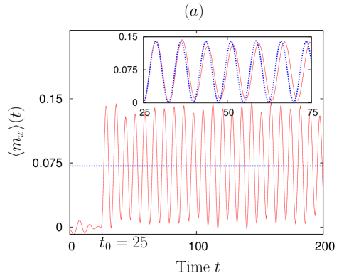
V.1 Linear response of homogeneous QSS: Single realization

The oscillatory behavior of $\langle m_{x}\rangle(t)$ predicted for the water-bag state, see formula (81), is checked in Fig. 1(a). Oscillations around a well-defined average persist indefinitely with no damping, as predicted by the theory. In the inset of the same panel, the theoretical prediction is compared with the numerical result for a few oscillations. While the agreement is quite good for the first two periods of the oscillations, the numerical data display a small frequency shift with respect to the theoretical prediction. Moreover, an amplitude modulation may also be observed. We have checked in our $N$-particle simulations that different initial realizations produce different frequency shifts, which has a consequence when averaging over an ensemble of initial realizations, as discussed below.

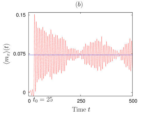
In Fig. 1(b), we show $\langle m_{x}\rangle(t)$ for the Fermi-Dirac QSS. In this case, we have the theoretical prediction only for the asymptotic value $\overline{m}_{x}$ given in Eq. (90). The time evolution of $\langle m_{x}\rangle(t)$ displays beatings and revivals of oscillations around this theoretical value, shown by the dashed horizontal line in the figure. There is no sign of asymptotic convergence, even running for longer times. For this high value of $\beta$, which makes the Fermi-Dirac distribution very close to the water-bag one, we cannot conclude that there will be damping in time. We have observed a damping for smaller values of $\beta$ when the Fermi-Dirac distribution comes closer to a Gaussian.

Figure 1: (Color online) $\langle m_{x}\rangle(t)$ vs. time $t$ for the (a) water-bag QSS, and (b) Fermi-Dirac QSS, in the HMF model under the action of the perturbation, Eqs. (61) and (63), with $h=0.1$ switched on at time $t_{0}=25$. (a) The full line in the main plot shows the result of $N$-particle simulation, while the dashed horizontal line is the theoretical time-averaged value of $\langle m_{x}\rangle(t)$ given in Eq. (82). The system size is $N=10^{5}$, while the parameter $p_{0}$, corresponding to energy $e=0.7$, is approximately $1.095$. In the inset, the numerical result (full line) is compared with the theoretical prediction (81) (dashed line). (b) The full line represents simulation results, while the horizontal dashed line is the theoretical asymptotic value given in Eq. (90). The system size is $N=10^{5}$, while $\beta=10$ and $\mu=1.2$, giving energy $e\approx 0.7$.

V.2 Linear response of the homogeneous equilibrium state: Single realization

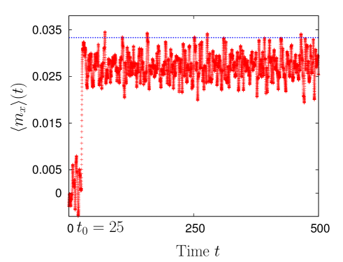
In Fig. 2, we show $\langle m_{x}\rangle(t)$ for the Gaussian QSS. After the application of the external field, the magnetization sharply increases and fluctuates around a value which is slightly below the theoretical prediction, Eq. (94). Convergence to this latter value is observed on longer times.

Figure 2: (Color online) $\langle m_{x}\rangle(t)$ vs. time $t$ for the Gaussian QSS in the HMF model under the action of the perturbation, Eqs. (61) and (63), with $h=0.1$ switched on at time $t_{0}=25$. The line made of pluses represents the result of $N$-particle simulation, while the dashed horizontal line is the theoretical asymptotic value given in Eq. (94). The system size is $N=10^{5}$, while $\beta=0.5$, so that the energy $e=1.5$.

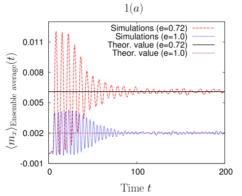
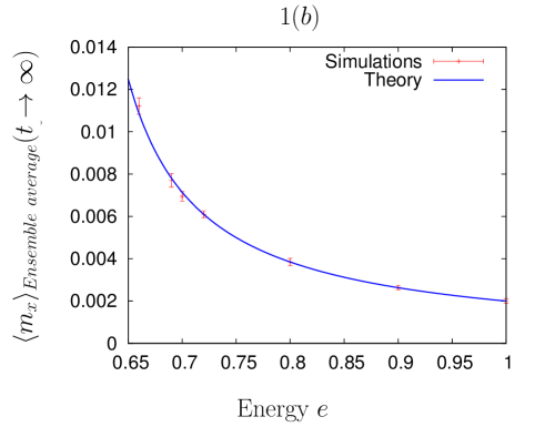
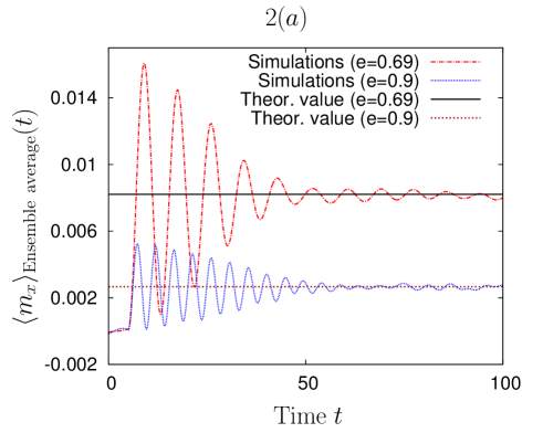
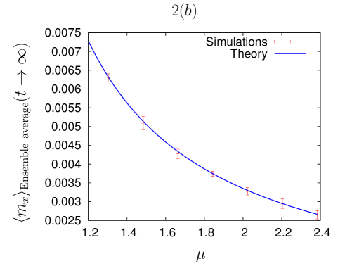
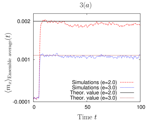
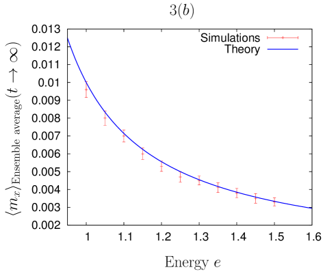
Figure 3: (Color online) Linear response of a water-bag QSS (panels 1(a), 1(b)), a Fermi-Dirac QSS with $\beta=10$ (panels 2(a), 2(b)), and the homogeneous equilibrium state (panels 3(a), 3(b)) for the HMF model under the perturbation, Eqs. (61) and (63), with $h=0.01$. All simulation data have been averaged over several thousand realizations of the initial state; for details, see text. In each case, panel (a) shows the time evolution of the averaged magnetization $\langle m_{x}\rangle_{\mbox{Ensemble average}}(t)$ as obtained from $N$-particle simulations, and its asymptotic approach either to the time average in Eq. (82) for the water-bag initial state or to $\overline{m}_{x}$ given in Eq. (90) for the Fermi-Dirac QSS, or to $\overline{m}_{x}$ given in Eq. (94) for the Gaussian QSS. In panel (b), we show the $N$-particle simulation results for the asymptotic magnetization as a function of energy (the parameter $\mu$ in the Fermi-Dirac case). The error bars denote the standard deviation of fluctuations around the asymptotic value. The results compare well with the theoretical predictions. The system size $N$ is $16,000$ for panels 1(a), 1(b) and panels 2(a), 2(b), and $10,000$ for panels 3(a), 3(b).

V.3 Average over initial realizations

In this section, we present numerical results for the three initial QSSs (water-bag, Fermi-Dirac, Gaussian), obtained after averaging the time evolution of $\langle m_{x}\rangle(t)$ over a set of realizations (typically a thousand) of the initial state. We define the average

$$\langle m_{x}\rangle_{\mbox{Ensemble average}}(t)=\frac{1}{N_{s}}\sum_{n=1}^{N_{s}}\langle m_{x}\rangle_{n}(t),$$ (99)

where $\langle\cdot\rangle_{n}$ labels the sample and $N_{s}$ is the total number of different realizations.

In all cases, we observe a relaxation to an asymptotic value. For the water-bag distribution, this value compares quite well with the time-averaged magnetization given in formula (82), see Fig. 3 panels (a) and (b). The mechanism by which the relaxation to the asymptotic value occurs in the water-bag case, in the absence of a true relaxation of a single initial realization, is the frequency shift present in the different initial realizations. This leads at a given time to an incoherent superposition of the oscillations of the magnetization. For other distributions, the numerically determined asymptotic value is compared with the theoretical value for the single realization $\overline{m}_{x}$, given in Eq. (90) and Fig. 3 panels 2(a) and 2(b), and formula (94) and Fig. 3 panels 3(a) and 3(b). The agreement is quite good.

V.4 Relaxation of QSS to equilibrium

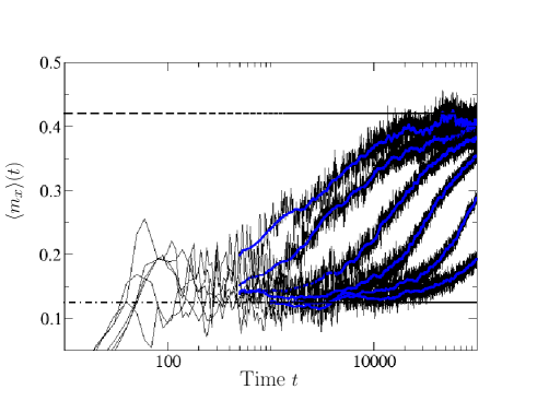
Figure 4: (Color online) Two-step relaxation of the water-bag QSS toward the Boltzmann-Gibbs equilibrium: $\langle m_{x}\rangle(t)$ vs. time $t$ for increasing system size from $N=2000$ to $N=64000$ (left to right). Under the perturbation, Eqs. (61) and (63) with $h=0.01$, the water-bag initial QSS with $e=0.65$ relaxes to an intermediate inhomogeneous QSS with $\langle m_{x}\rangle\approx 0.125$ (lower horizontal dash-dotted line) and then to the equilibrium state with $\langle m_{x}\rangle\approx 0.42$ (upper horizontal dashed line). The blue thick lines refer to running averages performed to smooth out local fluctuations.

For finite values of $N$, the perturbed HMF system finally relaxes to the Boltzmann-Gibbs equilibrium state. The presence of a two-step relaxation of the initial water-bag QSS with energy $e=0.65$, first to the perturbed Vlasov state and then to equilibrium, is shown in Fig. 4 for increasing system sizes for perturbation, Eqs. (61) and (63), with $h=0.01$. The relaxation to the first magnetization plateau with value $\approx 0.125$ predicted by the linear response theory takes place on a time of $O(1)$. The final relaxation to the equilibrium value of the magnetization $\approx 0.42$ occurs on a timescale that increases with system size, presumably with a power law that remains to be investigated further.

VI Concluding remarks

In this paper, we studied the response of a Hamiltonian long-range system in a quasistationary state (QSS) to an external perturbation. The perturbation couples to the canonical coordinates of the individual constituents. We pursued our study by analyzing the Vlasov equation for the time evolution of the single-particle phase space distribution. The QSSs represent stable stationary states of the Vlasov equation in the absence of the external perturbation. We linearized the perturbed Vlasov equation about the QSS for weak enough external perturbation to obtain a formal expression for the response observed in a single-particle dynamical quantity. For a QSS that is homogeneous in the coordinate, we derived a closed form expression for the response function. We applied this formalism to a paradigmatic model, the Hamiltonian mean-field model, and compared the theoretical prediction for three representative QSSs (the water-bag QSS, the Fermi-Dirac QSS and the Gaussian QSS) with $N$-particle simulations for large $N$. We also showed the long-time relaxation of the water-bag QSS to the Boltzmann-Gibbs equilibrium state.

VII Acknowledgments

S. G. and S. R. acknowledge support of the contract LORIS (ANR-10-CEXC-010-01). C. N. acknowledges support from the Ministère des Affaires Étrangères. Numerical simulations were done at the PSMN platform, ENS-Lyon. We acknowledge useful discussions with P. de Buyl, T. Dauxois, K. Gawedski, and especially, with F. Bouchet. We thank Yoshi Yamaguchi for discussions, for a careful reading of the manuscript, and for letting us know of a similar project he is pursuing on linear response.

Appendix A Normalization, energy density, and stability criterion for the Fermi-Dirac distribution [Eq. (83)]

Normalization: Consider the distribution Eq. (83). The normalization $A$ satisfies

$$A\int_{-\infty}^{\infty}\frac{dp}{1+e^{\beta(p^{2}-\mu)}}=1.$$ (100)

Changing variables and doing an integration by parts, we get

$$2\beta A\int_{0}^{\infty}dx~{}\frac{\sqrt{x}~{}e^{\beta(x-\mu)}}{\Big{[}1+e^{\beta(x-\mu)}\Big{]}^{2}}=1.$$ (101)

The left hand side may be written in terms of the derivative $\partial f_{\rm FD}(x)/\partial x$ of the Fermi-Dirac-like function $f_{\rm FD}(x)=1/[1+e^{\beta(x-\mu)}]$. We get

$$2A\int_{0}^{\infty}dx~{}\sqrt{x}\Big{(}\frac{-\partial f_{\rm FD}(x)}{\partial x}\Big{)}=1.$$ (102)

In the limit of large $\beta$, the derivative $\partial f_{\rm FD}(x)/\partial x$ approaches the Delta function: $\lim_{\beta\to\infty}\partial f_{\rm FD}(x)/\partial x=-\delta(x-\mu)$. In this limit, we may expand $\sqrt{x}$ in a Taylor series about $\mu$,

$$\sqrt{x}=\sqrt{\mu}+\frac{x-\mu}{2\sqrt{\mu}}-\frac{(x-\mu)^{2}}{8\mu^{3/2}}+\ldots,$$ (103)

which on substituting in Eq. (102) gives

$$A\Big{(}2\sqrt{\mu}I_{0}+\frac{1}{\beta\sqrt{\mu}}\mathcal{I}_{1}-\frac{1}{4\beta^{2}\mu^{3/2}}\mathcal{I}_{2}+\ldots\Big{)}=1.$$ (104)

Here,

$$\mathcal{I}_{0} = \int_{0}^{\infty}dx~{}\Big{(}\frac{-\partial f_{\rm FD}(x)}{\partial x}\Big{)}$$ (105)

$$= \int_{-\beta\mu}^{\infty}dy~{}\frac{e^{y}}{(1+e^{y})^{2}}$$

$$\stackrel{{\scriptstyle\beta\to\infty}}{{\longrightarrow}} \int_{-\infty}^{\infty}dy~{}\frac{e^{y}}{(1+e^{y})^{2}}=1,$$

$$\mathcal{I}_{1} = \beta\int_{0}^{\infty}dx~{}(x-\mu)\Big{(}\frac{-\partial f_{\rm FD}(x)}{\partial x}\Big{)}$$ (106)

$$= \int_{-\beta\mu}^{\infty}dy~{}\frac{ye^{y}}{(1+e^{y})^{2}}$$

$$\stackrel{{\scriptstyle\beta\to\infty}}{{\longrightarrow}} \int_{-\infty}^{\infty}dy~{}\frac{ye^{y}}{(1+e^{y})^{2}}=0,$$

$$\mathcal{I}_{2} = \beta^{2}\int_{0}^{\infty}dx~{}(x-\mu)^{2}\Big{(}\frac{-\partial f_{\rm FD}(x)}{\partial x}\Big{)}$$ (107)

$$= \int_{-\beta\mu}^{\infty}dy~{}\frac{y^{2}e^{2}}{(1+e^{y})^{2}}$$

$$\stackrel{{\scriptstyle\beta\to\infty}}{{\longrightarrow}} \int_{-\infty}^{\infty}dy~{}\frac{y^{2}e^{y}}{(1+e^{y})^{2}}=\frac{\pi^{2}}{3}.$$

Thus, to order $1/\beta^{2}$, we find from Eq. (104) that

$$A\Big{(}2\sqrt{\mu}-\frac{\pi^{2}}{12\beta^{2}\mu^{3/2}}\Big{)}=1,$$ (108)

which gives

$$A=\frac{1}{2\sqrt{\mu}}\Big{(}1+\frac{\pi^{2}}{24\beta^{2}\mu^{2}}\Big{)}.$$ (109)

Average energy: The average energy density is obtained from Eq. (57) as

$$e=A\int_{-\infty}^{\infty}dp~{}\frac{p^{2}/2}{1+e^{\beta(p^{2}-\mu)}}+\frac{1}{2}.$$ (110)

Changing variables and doing an integration by parts, we get

$$e=\frac{A}{3}\int_{0}^{\infty}dx~{}x^{3/2}\Big{(}\frac{-\partial f_{\rm FD}(x)}{\partial x}\Big{)}+\frac{1}{2}.$$ (111)

Expanding $x^{3/2}$ in a Taylor series about $\mu$ and substituting in Eq. (111) give

$$e = \frac{A}{3}\Big{(}\mu^{3/2}\mathcal{I}_{0}+\frac{3}{2\beta}\sqrt{\mu}\mathcal{I}_{1}+\frac{3}{8\beta^{2}\sqrt{\mu}}\mathcal{I}_{2}+\ldots\Big{)}+\frac{1}{2}$$ (112)

$$= \frac{A\mu^{3/2}}{3}\Big{(}1+\frac{\pi^{2}}{8\beta^{2}\mu^{2}}\Big{)}+\frac{1}{2}.$$

Using Eq. (109), we find that to $O(1/\beta^{2})$, the energy density is

$$e=\frac{\mu}{6}\Big{(}1+\frac{\pi^{2}}{6\beta^{2}\mu^{2}}\Big{)}+\frac{1}{2}.$$ (113)

Dielectric function: Using Eqs. (83) and (35), we get

$$\epsilon(1,0)=1-A\int_{0}^{\infty}dx~{}\frac{1}{\sqrt{x}}\Big{(}\frac{-\partial f_{\rm FD}(x)}{\partial x}\Big{)}.$$ (114)

Expanding $1/\sqrt{x}$ in a Taylor series about $\mu$, and substituting in Eq. (114) give

$$\epsilon(1,0)=1-A\Big{(}\frac{\mathcal{I}_{0}}{\sqrt{\mu}}-\frac{\mathcal{I}_{1}}{2\beta\mu^{3/2}}+\frac{3\mathcal{I}_{2}}{8\beta^{2}\mu^{5/2}}+\ldots\Big{)},$$ (115)

so that to $O(1/\beta^{2})$, we get

$$\epsilon(1,0)=1-\frac{1}{2\mu}\Big{(}1+\frac{\pi^{2}}{6\beta^{2}\mu^{2}}\Big{)},$$ (116)

where we have used Eq. (109).

References

• (1) A. Campa, T. Dauxois, and S. Ruffo, Phys. Rep. 480, 57 (2009).
• (2) Long-Range Interacting Systems, edited by T. Dauxois, S. Ruffo, and L. F. Cugliandolo (Oxford University Press, New York, 2010).
• (3) F. Bouchet, S. Gupta, and D. Mukamel, Physica A 389, 4389 (2010).
• (4) Y. Y. Yamaguchi, J. Barré, F. Bouchet, T. Dauxois, and S. Ruffo, Physica A 337, 36 (2004).
• (5) M. Joyce and T. Worrakitpoonpon, J. Stat. Mech.: Theory Exp. P10012 (2010); A. Gabrielli, M. Joyce, and B. Marcos, Phys. Rev. Lett. 105, 210602 (2010)
• (6) T. N. Teles, Y. Levin, R. Pakter, and F. B. Rizzato, J. Stat. Mech.: Theory Exp. P05007 (2010).
• (7) S. Gupta and D. Mukamel, J. Stat. Mech.: Theory Exp. P03015 (2011).
• (8) M. Antoni and S. Ruffo, Phys. Rev. E 52, 2361 (1995).
• (9) K. Jain, F. Bouchet, and D. Mukamel, J. Stat. Mech.: Theory Exp. P11008 (2007).
• (10) F. D. Nobre and C. Tsallis, Phys. Rev. E 68, 036115 (2003).
• (11) D. R. Nicholson, Introduction to Plasma Physics (Krieger Publishing Company, Florida, 1992).
• (12) L. Landau, J. Phys. USSR, 10, 25 (1946).
• (13) R. Kubo, J. Phys. Soc. Japan 12, 570 (1957).
• (14) M. Kac, G. E. Uhlenbeck, and P. C. Hemmer, J. Math. Phys. 4, 216 (1963).
• (15) W. Braun and K. Hepp, Comm. Math. Phys. 56, 101 (1977).
• (16) D. Ruelle, Nonlinearity 22, 855 (2009).
• (17) In this paper, we adopt the following convention to define spatial Fourier and temporal Laplace transforms: An arbitrary function F(q,p,t)𝐹𝑞𝑝𝑡F(q,p,t) of the canonical coordinate, momentum, and time has the spatial Fourier transform
F~(k,p,t)=12π𝑑qF(q,p,t)eikq,~𝐹𝑘𝑝𝑡12𝜋differential-d𝑞𝐹𝑞𝑝𝑡superscript𝑒𝑖𝑘𝑞\widetilde{F}(k,p,t)=\frac{1}{2\pi}\int dq~{}F(q,p,t)e^{-ikq},
so that the inverse Fourier transform is given by
F(q,p,t)=𝑑kF~(k,p,t)eikq.𝐹𝑞𝑝𝑡differential-d𝑘~𝐹𝑘𝑝𝑡superscript𝑒𝑖𝑘𝑞F(q,p,t)=\int dk~{}\widetilde{F}(k,p,t)e^{ikq}.
The temporal Laplace transform of F~(k,p,t)~𝐹𝑘𝑝𝑡\widetilde{F}(k,p,t) for t>0𝑡0t>0 is defined as
F^(k,p,ω)=0𝑑tF~(k,p,t)eiωt,^𝐹𝑘𝑝𝜔superscriptsubscript0differential-d𝑡~𝐹𝑘𝑝𝑡superscript𝑒𝑖𝜔𝑡\widehat{F}(k,p,\omega)=\int_{0}^{\infty}dt~{}\widetilde{F}(k,p,t)e^{i\omega t},
so that the inverse Laplace transform is given by
F~(k,p,t)=12πC𝑑ωF^(k,p,ω)eiωt,~𝐹𝑘𝑝𝑡12𝜋subscript𝐶differential-d𝜔^𝐹𝑘𝑝𝜔superscript𝑒𝑖𝜔𝑡\widetilde{F}(k,p,t)=\frac{1}{2\pi}\int_{C}d\omega~{}\widehat{F}(k,p,\omega)e^{-i\omega t},
where the Laplace contour C𝐶C is a horizontal line in the complex ω𝜔\omega-plane that passes above all singularities of F^(k,p,ω)^𝐹𝑘𝑝𝜔\widehat{F}(k,p,\omega).
• (18) P. H. Chavanis and L. Delfini, Eur. Phys. J. B 69, 389 (2009).
• (19) The model may also be interpreted as a mean-field XY𝑋𝑌XY model of magnetism, though this identification is only superficial in the sense that the dynamics (2) of the model is very different from that of XY𝑋𝑌XY spins Gupta:2011 .
• (20) V. Latora, A. Rapisarda, and S. Ruffo, Physica D 131, 38 (1999).
• (21) J. Barré, F. Bouchet, T. Dauxois, and S. Ruffo, J. Stat. Phys. 119, 677 (2005).
• (22) R. I. McLachlan and P. Atela, Nonlinearity 5, 541 (1992).
• (23) E. Caglioti and F. Rousset, J. Stat. Phys. 129, 241 (2007); E. Caglioti and F. Rousset, Arch. Rational Mech. Anal. 190, 517 (2008).