Resolving multiple supermassive black hole binaries with pulsar timing arrays

Abstract

We study the capability of a pulsar timing array (PTA) to individually resolve and localize in the sky monochromatic gravitational wave (GW) sources. Given a cosmological population of inspiralling massive black hole binaries, their observable signal in the PTA domain is expected to be a superposition of several nearly-monochromatic GWs of different strength. In each frequency bin, the signal is neither a stochastic background nor perfectly resolvable in its individual components. In this context, it is crucial to explore how the information encoded in the spatial distribution of the array of pulsars might help recovering the origin of the GW signal, by resolving individually and locating in the sky the strongest sources. In this paper we develop a maximum-likelihood based method finalized to this purpose. We test the algorithm against noiseless data showing that up to $P/3$ sources can be resolved and localized in the sky by an array of $P$ pulsars. We validate the code by performing blind searches on both noiseless and noisy data containing an unknown number of signals with different strengths. Even without employing any proper search algorithm, our analysis procedure performs well, recovering and correctly locating in the sky almost all the injected sources.

I Introduction

Within this decade the detection of gravitational waves (GWs) may be a reality, opening a completely new window on the Universe. Precision timing of millisecond pulsars within a pulsar timing array (PTA) provides a unique opportunity to get the very first low-frequency GW detection. GWs affect the propagation of radio signals from the pulsar to the receiver on Earth, leaving a characteristic fingerprint in the time of arrival of the radio pulses (e.g., sazhin78, ; hellings83, ). This technique is particularly sensitive in the $10^{-9}-10^{-7}$Hz window, where genuinely supermassive black hole binaries (SMBHBs, $10^{8}-10^{9}\,{\rm M_{\odot}}$) at low redshift ($z<2$) will dominate the signal (Sesana et al. 2009). The Parkes Pulsar Timing Array (PPTA,  manchester2008, ), the European Pulsar Timing Array (EPTA,  janssen2008, ) and the North American Nanohertz Observatory for Gravitational Waves (NANOGrav,  jenet2009, ), joining together in the International Pulsar Timing Array (IPTA,  hobbs2010, ), are already collecting data and improving their sensitivity in the frequency range of $\sim 10^{-9}-10^{-6}$ Hz. In the coming years, the Chinese five hundred meter aperture spherical telescope (FAST,  smits09, ) and the planned Square Kilometer Array (SKA,  lazio2009, ) will provide a major leap in sensitivity.

The signal expected from a cosmological population of inspiralling SMBHBs consists of a superposition of quasi-monochromatic waves, similar to the white dwarf-white dwarf foreground (e.g., Nelemans01, ) in the mHz window relevant to space based interferometry. Such signal can be divided into two distinct contributions: (i) a stochastic background generated by the incoherent superposition of radiation from the whole SMBHB population rr95 ; jaffe03 ; sesana08 and (ii) individually resolvable, deterministic signals produced by single sources that are sufficiently massive and/or close so that the gravitational signal stands above the root-mean-square (rms) level of the background sesana09 . Accordingly, signal recovery and data analysis investigations have been developed in the limiting cases of either an isotropic stochastic background described by a power-law spectrum jen05 ; jen06 ; anholm09 ; vanh09 ; vanh11 , or of a single GW source jen04 ; SesanaVecchio10 ; corbin2010 ; yardley10 ; lee11 .

The actual expected signal, however, is far from being isotropically distributed in the sky, with just few sources dominating the power at each frequency sesana08 ; KS11 . The GW signal generated by an astrophysically motivated SMBHB population is neither isotropic and stochastic, nor dominated by a single source. It is therefore important to fully characterize such signal, and to assess how much of the information enclosed in it can be recovered. It is, in fact, not clear a priori how such inhomogeneous combination of multiple sources emitting in the same frequency bin will appear in the time residuals: whether they will look almost isotropic over the sky, or they will superpose and appear as a single one, or as few bright spots in the sky.

This paper is a proof of concept of how the spatial information enclosed in a PTA can be exploited to disentangle a superposition of signals coming from different directions in the sky. We utilize a maximum-likelihood based algorithm designed to identify the sky origin and relative strengths of a collection of incoherently superposed monochromatic signals. We test the algorithm performances on different noiseless datasets, and then we apply it to noisy datasets. In agreement with simple counting arguments and with previous analytical results boyle10 we find that $P/3$ sources can be resolved and localized in the sky by an array of $P$ pulsars. If the number of sources is more than $P/3$ we might identify the presence of extra sources with poor localization precision, and we will not be able to estimate their parameters. When few sources are present, the maximum likelihood estimator allows to infer the correct number of contributing sources, and the algorithm locates them in the sky with good accuracy. The same is true when noise is added to the data. Also in a situation of source SNR$\approx 10$, the algorithm is able to correctly disentangle signals and to locate the sources in the sky.

This pilot study demonstrates the potential of PTAs of resolving and locating in the sky a sizable number of sources. We stress that we do not implement any proper search algorithm when looking for solutions that maximize the likelihood estimator, and we do not draw sources from expected astrophysical SMBHB populations. We plan to consider these aspects of the problem in the future, to test our method under more realistic assumptions.

The paper is organized as follows. We spell out the objectives and the assumptions of our data analysis method in Section II. The model used for the sources and a detailed mathematical description of the detection strategy can be found in Section III. We discuss source identification and resolvability in Section IV and test our method against blind datasets in Section V. We summarize and discuss future research directions in Section VI.

II Objectives and basic assumptions

The main aim of this paper is to provide a proof of concept of the potential of PTAs to resolve individual contributions to a GW signal formed by the incoherent superposition of several monochromatic sources. We are primarily interested here in disentangling the source contribution to the signal and in estimating their sky location. As we aim at a proof of concept, we make a set of simplifying assumptions:

1. only GW sources contribute to the timing residuals, i.e., we test our method on noiseless data. We will relax this assumption in the last Section, testing the effectiveness of our technique on noisy synthetic data. When included, noise is modelled as white and Gaussian, with equal magnitude in all the pulsars forming the array;

2. we only consider few GW sources contributing to the data streams. We will consider more realistic source populations where few bright sources might dominate over a large distribution of weaker ones in future investigations;

3. we look at signals in a particular ‘frequency bin’, i.e, we do not perform any frequency search. Throughout the paper we deal with monochromatic signals at $f=14$ nHz ($f=20$ nHz for the blind challenges). We assume that the frequency is known. We intend to include frequency scanning in the analysis in forthcoming studies;

4. when modelling the GW signal, we use the leading quadrupole approximation for non-spinning binaries in quasi-circular orbit, as we will describe in the details in Section III;

5. we consider the “Earth” term only in the pulsar response, excluding the “pulsar” term. GW sources aligned along the Earth-pulsar line of sight do not contribute to the timing residuals if the full response is considered (Earth$+$pulsar terms), however excluding the “pulsar” term makes the response infinite in this case. We therefore exclude GW sources within 5 degrees of any pulsar sky location. We will give more details on the “pulsar” and the “Earth” terms in Section III;

6. the sky location of the pulsars in the array is drawn from a uniform distribution on the sphere;

7. we assume 10 years of uninterrupted equally-sampled (once every two weeks) observations of each pulsar in the array;

8. we do not implement any proper search algorithm in maximizing the likelihood. The sky maps and maximum likelihood estimates are computed by randomly (uniformly on the sphere) drawing points in the sky. We will optimize the search algorithm in future investigations.

Each residual series is monochromatic in our set up, and therefore contains two measurable quantities: the amplitude and the initial phase. On the other hand, in the approximation of circular non evolving sources, the GW signal is described by six parameters: overall amplitude ${\cal A}$, inclination $\iota$, initial orbital phase $\Phi_{0}$, polarization angle $\psi$, sky location angles $\{\phi,\theta\}$. The simple counting of the measurable quantities (two per pulsar) and of the number of unknowns (six per GW source) suggests that we will need $P=3\times N$ pulsars to detect and to estimate parameters of $N$ GW sources. In general this counting is correct if one knows the exact number of signals in the data and wants to estimate parameters of all these signals. In a real situation the exact number of GW signals is unknown. In addition the strength of different GW sources could vary significantly, with a large fraction of weak sources forming an anisotropic (in the sky) background for the brighter ones.

III GW source model and detection strategy

The analysis is built around the maximum likelihood estimator of the source parameters. We notice that the likelihood could be maximized analytically over some (what are called extrinsic) parameters characterizing the GW source, in a way similar to the $F$-statistic JKS . We therefore need to write the signal in a mathematical form suitable to such analytical maximization.

III.1 Gravitational wave model

We consider monochromatic GW sources assuming that the orbital frequency does not change appreciably over the observation period (see, e.g., SesanaVecchio10, ) which we took to be 10 years. The signal is characterized by the six parameters introduced in the previous Section $\{{\cal A},\iota,\Phi_{0},\psi,\phi,\theta\}$, plus the GW frequency $f$, which we assume to be known here. Those parameters describe the GW signal from a widely separated SMBHB in quasi-circular orbit. We neglect all modulations due to spin-orbital coupling vecchio04 , so effectively we consider two non-spinning SMBHs. We refer the reader for more detailed discussion on the waveforms and on the computing the timing residuals to SesanaVecchio10 . The waveform in the radiative frame reads

$$h_{ij} = \epsilon_{ij}^{+}h_{+}+\epsilon_{ij}^{\times}h_{\times},$$ (1)

$$\epsilon_{ij}^{+} = p_{i}p_{j}-q_{i}q_{j},\;\;\;\epsilon_{ij}^{\times}=p_{i}q_{j}+p_{j}q_{i},$$ (2)

where $\hat{p},\hat{q}$ is the polarization basis. The polarization basis associated to the Earth (or to the Solar system barycenter) is

$$\hat{u} = \{\cos{\theta}\cos{\phi},\cos{\theta}\sin{\phi},-\sin{\theta}\},$$ (3)

$$\hat{v} = \{\sin{\phi},-\cos{\phi},0\},$$ (4)

$$\hat{p} = \hat{u}\cos{\psi}-\hat{v}\sin{\psi},\;\;\;\hat{q}=\hat{v}\cos{\psi}+\hat{u}\sin{\psi}.$$ (5)

The rotation in the last line defines the polarization angle $\psi$. The components of the GW signal are

$$h_{+} = \mathcal{A}(1+\cos^{2}{\iota})\cos(\Phi(t)+\Phi_{0})$$

$$h_{\times} = -2\mathcal{A}\cos{\iota}\sin(\Phi(t)+\Phi_{0})$$ (6)

where we have written explicitly the initial GW phase, and

$$\mathcal{A}=2\frac{\mathcal{M}_{c}^{5/3}}{D_{L}}(\pi f)^{2/3}.$$ (7)

In the last equation $\mathcal{M}_{c}=M_{1}^{3/5}M_{2}^{3/5}/(M_{1}+M_{2})^{1/5}$ is the chirp mass of the source, and $D_{L}$ is its luminosity distance. The residuals in the arrival time of the radio pulses due to the propagation of the electromagnetic waves in the field of the GW can be written as

$$r(t)=\int_{0}^{t}\frac{\delta\nu}{\nu}(t^{\prime})dt^{\prime},$$ (8)

$$\frac{\delta\nu}{\nu}=\frac{1}{2}\frac{\hat{n}^{i}\hat{n}^{j}}{1+\hat{n}\cdot\hat{k}}\Delta h_{ij},$$ (9)

where $\hat{n}$ denotes the position of the pulsar on the sky, and $\hat{k}$ is the direction of the GW propagation. The last term depends on the strain of the GW at the location of the pulsar $h_{ij}(t_{p})$ and at the Earth $h_{ij}(t)$:

$$\Delta h_{ij}=h_{ij}(t_{p})-h_{ij}(t).$$ (10)

Since the pulsars are not correlated ($t_{p}$, the emission time of the pulse detected at the time $t$ on the Earth, is different for all pulsars) the “pulsar” terms do not add up coherently and for this work we will neglect them and concentrate on the “Earth” terms only. The pulsar terms can be considered as part of the noise, which for the time being we do not include in our analysis. Substituting equation (III.1) into equation (8), the Earth part of the residual is written as

$$r_{\alpha}^{E}(t)=\frac{\mathcal{A}}{2\pi f}\left\{(1+\cos^{2}{\iota})F_{\alpha}^{+}\left[\sin(\Phi(t)+\Phi_{0})-\sin{\Phi_{0}}\right]+\right.$$

$$\left.2\cos{\iota}F_{\alpha}^{\times}\left[\cos(\Phi(t)+\Phi_{0})-\cos{\Phi_{0}}\right]\right\},$$ (11)

where the index $\alpha$ refers to a particular pulsar in the array, and the antenna-response functions are

$$F_{\alpha}^{+} = \frac{1}{2}\frac{(\hat{n}^{\alpha}\cdot\hat{p})^{2}-(\hat{n}^{\alpha}\cdot\hat{q})^{2}}{1+\hat{n}^{\alpha}\cdot\hat{k}}$$ (12)

$$F_{\alpha}^{\times} = \frac{(\hat{n}^{\alpha}\cdot\hat{p})(\hat{n}^{\alpha}\cdot\hat{q})}{1+\hat{n}^{\alpha}\cdot\hat{k}}.$$ (13)

It is convenient to rewrite the above expressions isolating the terms containing the polarization angle:

$$F_{\alpha}^{+} = F^{\alpha}_{c}\cos(2\psi)+F^{\alpha}_{s}\sin(2\psi)$$ (14)

$$F_{\alpha}^{\times} = -F^{\alpha}_{s}\cos(2\psi)+F^{\alpha}_{c}\sin(2\psi)$$ (15)

where

$$F^{\alpha}_{c} = \left\{-\frac{1}{4}(\sin^{2}(\chi_{\alpha})-2\cos^{2}(\chi_{\alpha}))\sin^{2}(\theta)-\right.$$

$$\left.\frac{1}{2}\cos(\chi_{\alpha})\sin(\chi_{\alpha})\sin(2\theta)\cos(\phi-\gamma_{\alpha})+\right.$$

$$\left.\frac{1}{4}(1+\cos^{2}(\theta))\sin^{2}(\chi_{\alpha})\cos(2\phi-2\gamma_{\alpha})\right\}\frac{1}{1+\hat{n}^{\alpha}\cdot\hat{k}}$$

$$F^{\alpha}_{s} = \left\{\cos(\chi_{\alpha})\sin(\chi_{\alpha})\sin(\theta)\sin(\phi-\gamma_{\alpha})+\right.$$ (16)

$$\left.\frac{1}{2}\sin^{2}(\chi_{\alpha})\cos(\theta)\sin(2\gamma_{\alpha}-2\phi)\right\}\frac{1}{1+\hat{n}^{\alpha}\cdot\hat{k}}.$$

Note that $F^{\alpha}_{c}$ and $F^{\alpha}_{s}$ depend only on the sky locations of the pulsar $\{\gamma_{\alpha},\chi_{\alpha}\}$ and of the GW source $\{\phi,\theta\}$. Using these expressions we can rewrite the residuals as

$$r_{\alpha}^{E}(t)=\sum_{j=1}^{4}a_{(j)}h_{(j)}^{\alpha},$$ (17)

where

$$h_{(1)}=F^{\alpha}_{c}\sin[\Phi(t)],\;\;\;h_{(2)}=F^{\alpha}_{s}\sin[\Phi(t)],$$

$$h_{(3)}=F^{\alpha}_{c}\cos[\Phi(t)],\;\;\;h_{(4)}=F^{\alpha}_{s}\cos[\Phi(t)],$$ (18)

and

$$a_{(1)}=\frac{\mathcal{A}}{2\pi f}[(1+\cos^{2}{\iota})\cos(2\psi)\cos(\Phi_{0})-2\cos{\iota}\sin(2\psi)\sin(\Phi_{0})],$$

$$a_{(2)}=\frac{\mathcal{A}}{2\pi f}[(1+\cos^{2}{\iota})\sin(2\psi)\cos(\Phi_{0})+2\cos{\iota}\cos(2\psi)\sin(\Phi_{0})],$$

$$a_{(3)}=\frac{\mathcal{A}}{2\pi f}[(1+\cos^{2}{\iota})\cos(2\psi)\sin(\Phi_{0})+2\cos{\iota}\sin(2\psi)\cos(\Phi_{0})],$$

$$a_{(4)}=\frac{\mathcal{A}}{2\pi f}[(1+\cos^{2}{\iota})\sin(2\psi)\sin(\Phi_{0})-2\cos{\iota}\cos(2\psi)\cos(\Phi_{0})].$$

III.2 Detection strategy

We have now brought the timing residuals into a form that allows analytic maximization of the likelihood (to be introduced in the next paragraph) over the parameters $a_{(i)}$, in a way similar to the $F$-statistic. We introduce the inner product:

$$<x|h>\equiv\frac{T_{o}}{S(f)}(x||h),\;\;\;(x||h)\equiv\frac{2}{T_{o}}\int_{0}^{T_{o}}x(t)h(t)dt,$$ (19)

where $T_{o}$ is the observation timespan and $S(f)$ is the two-sided noise spectral density.

Consider now a dataset $x_{\alpha}$; the log-likelihood that this dataset contains a GW signal $r_{\alpha}(t;\vec{\lambda})$ , where $\vec{\lambda}$ is a vector of GW parameters describing the signal, is

$$\log{\Lambda_{\alpha}}\sim<x_{\alpha}|r_{\alpha}>-\frac{1}{2}<r_{\alpha}|r_{\alpha}>\sim(x_{\alpha}||r_{\alpha})-\frac{1}{2}(r_{\alpha}||r_{\alpha}).$$ (20)

Since we consider monochromatic sources and noise-less data, $S(f)$ is just a scaling constant in our calculations; in the following, we neglect numerical coefficients, and we compute scaled log-likelihoods. Let us now assume we have a collection of datasets $x_{\alpha}$, $\alpha=1,...,P$, corresponding to observations of $P$-pulsars, and let us infer that a single GW is present in the datasets. The total log-likelihood evaluated on the $P$ datasets is simply the sum of the individual log-likelihoods, and substituting $r_{\alpha}$ given in equation (17) into equation (20), can be written as:

$$\log(\Lambda) = \sum_{\alpha=1}^{P}\log(\Lambda_{\alpha})$$ (21)

$$\sim \sum_{j=1}^{4}a_{(j)}X_{j}-\frac{1}{2}\sum_{j=1}^{4}\sum_{k=1}^{4}a_{(j)}a_{(k)}M_{jk},$$

where

$$X_{j}\equiv\sum_{\alpha=1}^{P}(x_{\alpha}||h^{\alpha}_{(j)}),\;\;\;\;M_{jk}\equiv\sum_{\alpha=1}^{P}(h_{(j)}^{\alpha}||h_{(k)}^{\alpha})$$ (22)

As in the $F$-statistics case, we can maximize the log-likelihood over the extrinsic parameters $a_{(j)}$:

$$\frac{\partial\log(\Lambda)}{\partial a_{(j)}}=0,\;\;\;\;\to a_{(k)}=M^{-1}_{kj}X_{j},$$ (23)

$$\{\log(\Lambda)\}_{{\rm max}\{a_{(j)}\}}=\frac{1}{2}X_{k}M^{-1}_{jk}X_{j}$$ (24)

where the sum over the repeated indices $j,k=1,...,4$ is assumed. Note that such maximization absorbs the four parameters ${\cal A}$, $\iota$, $\psi$ and $\Phi_{0}$; the maximized log-likelihood has therefore a form similar to the $F$-statistic and (for a fixed frequency) is function of the sky location $\{\phi,\theta\}$ of the GW source only. From now on, when we talk about log-likelihood, we mean log-likelihood maximized over $a_{(j)}$ according to equations (23) and (24), and for an individual GW source is a function of two parameters only. The $M$-matrix is block-diagonal, and is given by

$$M_{jk}=\sum_{\alpha}\left(\begin{array}[]{cccc}(F^{\alpha}_{c})^{2}&F^{\alpha}_{c}F_{\alpha}^{s}&0&0\\ F^{\alpha}_{c}F^{\alpha}_{s}&(F^{\alpha}_{s})^{2}&0&0\\ 0&0&(F^{\alpha}_{c})^{2}&F^{\alpha}_{c}F^{\alpha}_{s}\\ 0&0&F^{\alpha}_{c}F^{\alpha}_{s}&(F^{\alpha}_{s})^{2}\end{array}\right).$$ (29)

Clearly one does not know a priori how many GW sources contribute to the dataset; the extension of the model to $N$ sources is mathematically straightforward. For each source we simply have four $a_{(j)}$ coefficients, meaning that all the summations in equations (21) and (22) have to be performed over $j,k=1,...,4N$. Now the coefficients $a_{(j)}$ become a $4\times N$ array, $X_{j}$ is also a $4\times N$ array, while the $M$-matrix is now a $4N\times 4N$, 2-D matrix

$$M_{jk}=\sum_{\alpha=1}^{P}(h_{(j)}^{\alpha}||h_{(k)}^{\alpha}).$$ (30)

(where indices $j,k$ run over $1,...,4N$) and it takes into account for correlations between the different GW signals.

When considering a multi-source model we can also estimate the relative contribution of each individual source to the overall likelihood estimator. For each source the analytical maximization of the likelihood according to equation (23) provides an estimate of the four parameters characterizing the waveform. The relative contribution of each source to the maximum likelihood solution normalized to the strongest source can therefore be written as

$$C_{n}=\log(\Lambda)\frac{\sqrt{\sum_{j=1}^{4}{(a_{(j)}^{n})^{2}}}}{{\rm max}_{m}\left(\sqrt{\sum_{j=1}^{4}{(a_{(j)}^{m}})^{2}}\right)}$$ (31)

where $n,m=1,...,N$. In the above expression ${\rm max}_{m}$ identifies the brightest source in the dataset, and the sums are over the four coefficients of each $n$ source. Note that $C_{n}$ is a function of the source inclination and of the overall GW amplitude, and is proportional to $\sqrt{h_{+}^{2}+h_{\times}^{2}}$, as introduced in equation (III.1). Note that in this definition, if we have identical GW sources but at different sky locations, then all the individual $C_{n}$ are the same and are equal to the total likelihood.

In the following sections we will perform a search of the GW source sky locations by maximizing the log-likelihood given by equation (21). We will compute the log-likelihood assuming a variable number of GW sources contributing to the residuals, to check whether our analysis allows us to infer the correct number of sources present in the dataset. As a result the log-likelihood parameter space is generally a function of $2\times N$ parameters, corresponding to the sky locations of the $N$ GW sources. In plotting multi-source sky maps we will usually show regions of the parameter space which are within 10 % of the maximum likelihood, and we will call them ambiguity or error regions. Actual ambiguity regions depend on the SNR of the GW signals, and are therefore meaningless in the noise-less case, nevertheless we think that the introduced error regions are still useful to indicate the degeneracies/ambiguities in the parameter space.

IV Testing the algorithm performance

In this section we apply the theory outlined above to some test cases to assess its effectiveness in resolving individual sources (and dependence on the number of sources and on the number of pulsars in the array used for detection). We consider here the limit of few GW sources present in the dataset; extension of the analysis to a realistic population of sources is deferred to future investigations.

IV.1 Minimum requirements for source localization

We first test the statement that $3N$ pulsars are required to resolve $N$ GW sources. We start by considering one GW source and one pulsar and we add pulsars and sources one by one to see how the likelihood pattern describing the source sky location changes. We start by injecting a first source at a location $\{4.26,0.78\}$, then we add a second source at a location $\{1.50,1.52\}$. Pulsars are placed randomly in the sky.

Figure 1: Log-likelihood sky map for the sky position of the GW source (black star), in a detection with three pulsars (green circles). Note that only relative values of the log-likelihood are meaningful. The best estimate for the source position is $\{4.27,0.78\}$, whereas the true one is $\{4.26,0.78\}$.

• One GW signal and one pulsar. In this case we might only say whether the GW signal is present or not. Our method cannot estimate the parameters of the source. Mathematically this correspond to a singular (determinant equal to zero) $M$-matrix.

• One GW signals and two pulsars. With two pulsars we can estimate four parameters but we cannot get any information about the sky position: $\Lambda(\phi,\theta)=const$, with the exact value depending on the relative position of the pulsars and the source.

• One GW signal and three pulsars. Finally, we have enough measurable quantities to estimate the position of the source on the sky. The accuracy depends on the relative position of the pulsars and the source. In figure 1 we give an example of the log-likelihood map of the source sky position. The shape and area of the likelihood peak strongly depend on the relative position of the source and the pulsars. The presence of the noise will make the picture worse by (possibly) promoting false local maxima. Conversely, adding more pulsars significantly improves the accuracy of the localization.

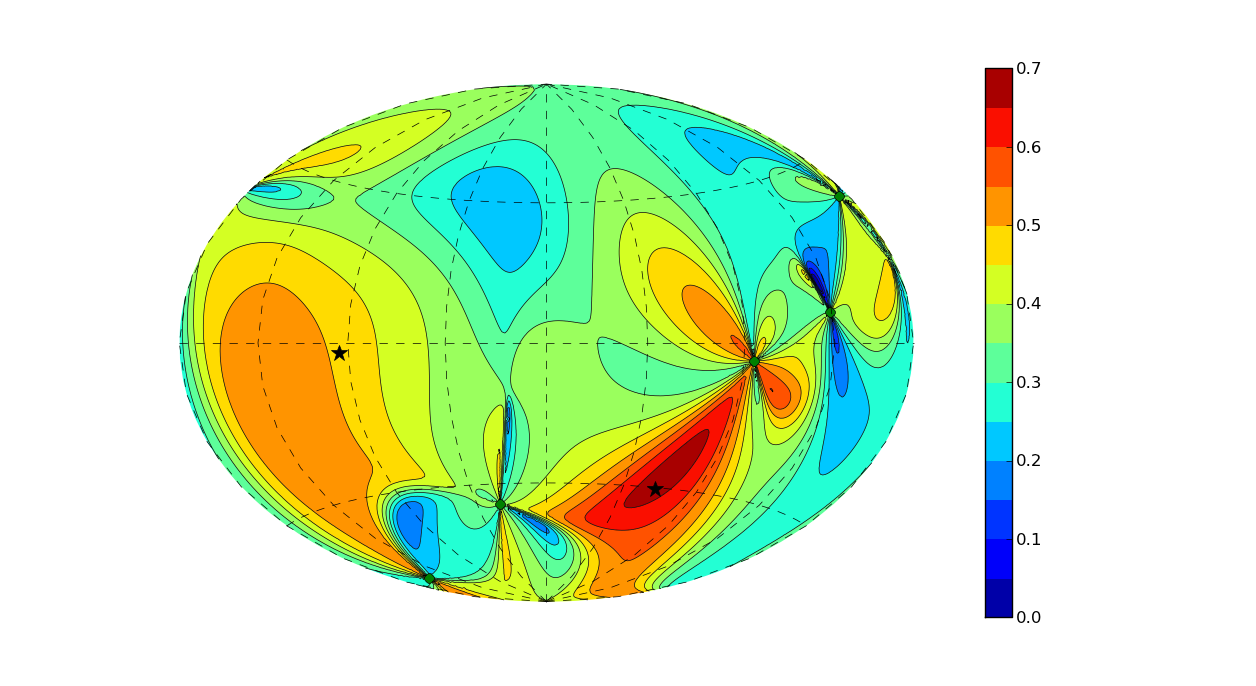
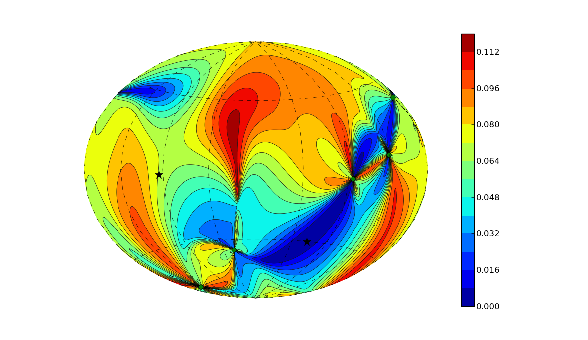
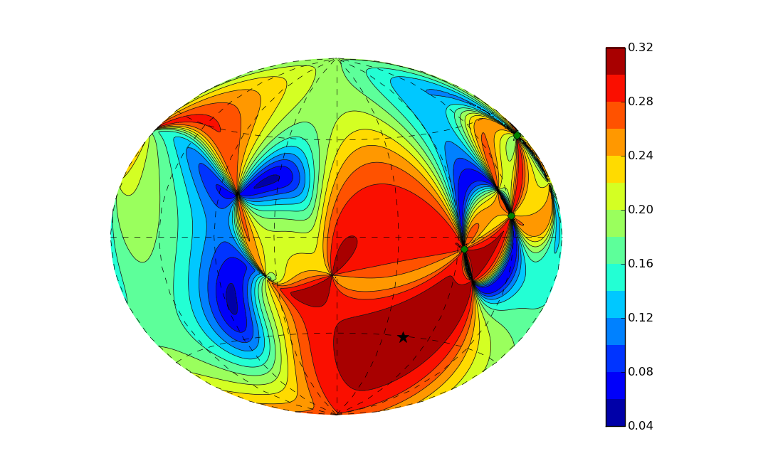
  Figure 2: Top panel: five pulsars (green circles) and two sources (black stars): the source log-likelihood map is constructed assuming a one source model, whereas there are two sources in the dataset. The best source position estimate is $\{4.33,0.89\}$; the true positions of the sources are $\{1.50,1.52\}$ and $\{4.26,0.78\}$. Bottom panel: log-likelihood map, assuming a single GW source, constructed after the removal of the best estimate shown in the top panel. Although there are hints of the presence of a second source, its inferred sky location does not match the actual position of the second GW source at $\{1.50,1.52\}$.

• Two GW signals and three pulsars. We do not have enough measured quantities to determine the parameters of both GW sources; again, the $M$-matrix is degenerate. However we can compute the likelihood map assuming that there is only one GW source contributing to the measured timing residuals. The result depends on the strength of the GW signals (both on the intrinsic strength and on the pulsar response function, i.e., on the relative source-pulsar sky location). We tested the most degenerate case: we took two identical GW sources, and we placed them at different sky locations ($\{4.26,0.78\}$, $\{1.50,1.52\}$). Not surprisingly, being the signal a superposition of two monochromatic plane waves, the two sources show up like a single one at a midway sky location. Adding a forth pulsar does not significantly improve the situation.

• Two GW signals and five pulsars. Still we do not have enough measured quantities (10) to measure all the source parameters (12). However, in a single GW source model, we start to see evidence of two likelihood maxima for the source sky location, a strong indication that there is more than one source. As shown in the upper panel of figure 2, we now resolve one source and we have a large local maximum next to the second one. The result varies with the relative source-pulsar position, but for fixed (chosen above) positions of the GW sources we usually resolve one source or the other. In addition we have computed the log-likelihood map assuming two GW sources in the data. Since we still do not have enough measurements to estimate all the parameters, the likelihood forms a complicated pattern in the sky reflecting this degeneracy. However the value of the log-likelihood for the two-source model is higher (by about 13%) than the single source model, strongly favoring the presence of two signals in the data. To further check what can be possibly done in this situation, we have tried to take the best estimate obtained by the single-source model, subtract it from the dataset and re-analyze it again searching for the second GW source (using again a single-source model). Unfortunately the procedure does not work well. The maximum likelihood estimators of the amplitude parameters of the first source have large errors (estimated values are $a_{(i)}=\{6.15,-1.71,-5.44,-2.57\}\times 10^{-10}$ instead of the correct values: $a^{true}_{(i)}=\{4.08,-2.54,-2.53,-4.09\}\times 10^{-10}$): when subtracting it, we are effectively partially removing the second GW source. The result after the removal is shown in the lower panel of figure 2. There is an indication of a second GW signal but it is in a completely wrong location. We can conclude that in an array of five pulsars there is enough information to identify the presence of two sources, but it is impossible to correctly localize both of them in the sky.

  

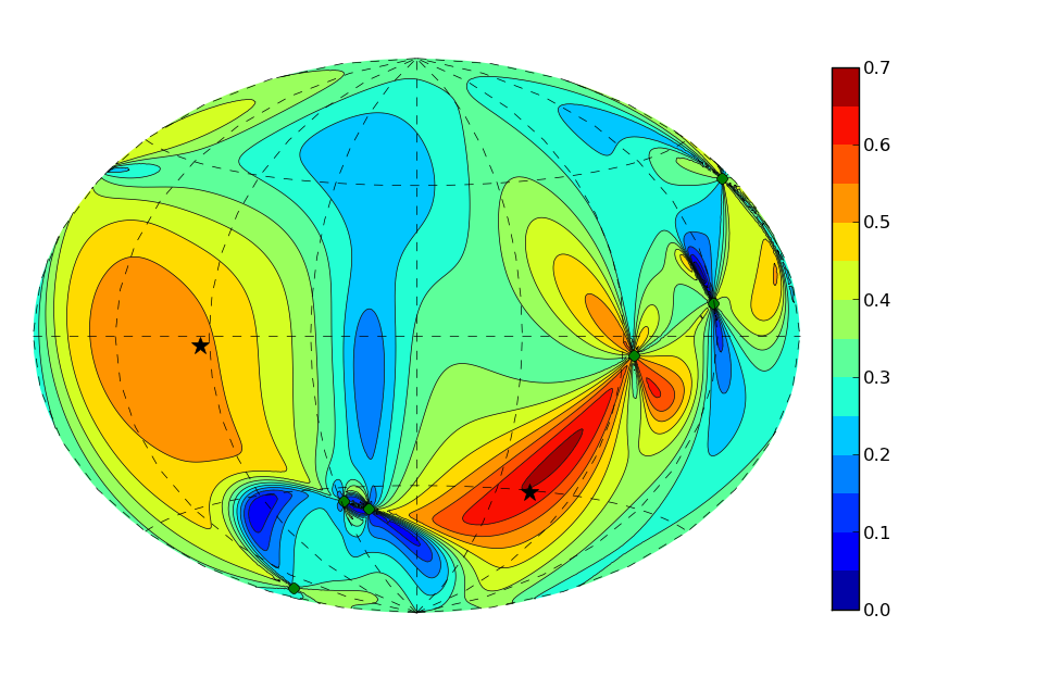
  Figure 3: Same as the top panel of figure 2, but now using six pulsars for the detection. The log-likelihood map clearly shows two extended maxima around the true location of the sources. The best single source sky location estimate is $\{4.35,0.94\}$, the true positions are the same as in figure 2.

• Two GW signals and six pulsars. Finally we have enough pulsars to estimate all the GW parameters, however the randomly chosen sixth pulsar is quite close to one of the previous five, so some level of degeneracy remains. The log-likelihood contour plot for the single source model shown in figure 3 clearly has two maxima centered at the true location of the sources. We also successfully tested a two source model: the pair of points in the sky which returned the highest log-likelihood were $\{1.48,1.55\},\{4.31,0.78\}$, close to the true values.

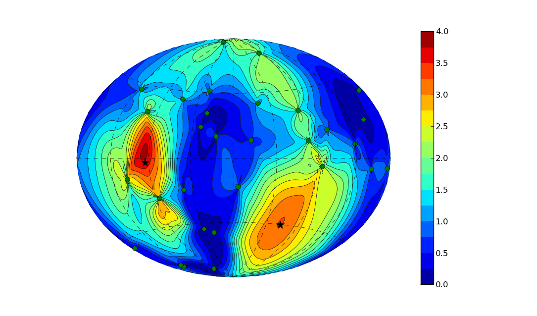
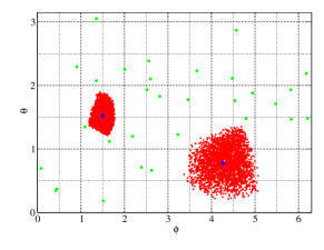
  Figure 4: Top panel: same as in figure 2, but now using 30 pulsars for the detection. The best single source position estimate is now shifted to the other source, and the inferred location is $\{1.48,1.63\}$, whereas the true position is $\{1.50,1.52\}$. Bottom panel: log-likelihood map assuming that there are two GW sources (blue diamonds), with measurements from 30 pulsars (green circles). We have selected all the pairs of points which are within 10% of the maximum likelihood estimate. The best source sky location estimates are $\{1.48,1.55\},\{4.31,0.78\}$, whereas the true positions are $\{1.50,1.52\},\{4.26,0.78\}$.

• Two GW signals and thirty pulsars. By adding pulsars to the array, uncertainty regions shrink and secondary maxima disappear. Here is an example of what we would see with data from 30 pulsars. The log-likelihood contour plot for the single source model shown in the top panel of figure 4 nails down the true location of the sources. We plot the results of a two source model in the lower panel of figure 4. In this case, the likelihood is a function of four parameters (the angles defining the sky location of the two sources) and a visual representation is not straightforward. We randomly choose pair of points in the sky and computed the log-likelihood. In the figure we plot all the pair of points which are within 10% of the maximum likelihood estimate (note that a 10% drop in the log-likelihood roughly corresponds to the uncertainty region of a pair of sources with combined SNR$=10$).

IV.2 Resolving a cluster of GW sources

Figure 5: Detection of a cluster of sources (black stars in each plot). The log-likelihood sky map for a single source model is shown, assuming detection with 6 (top) and 100 (bottom) pulsars (green circles). The color coding corresponds to the (scaled) log-likelihood value.

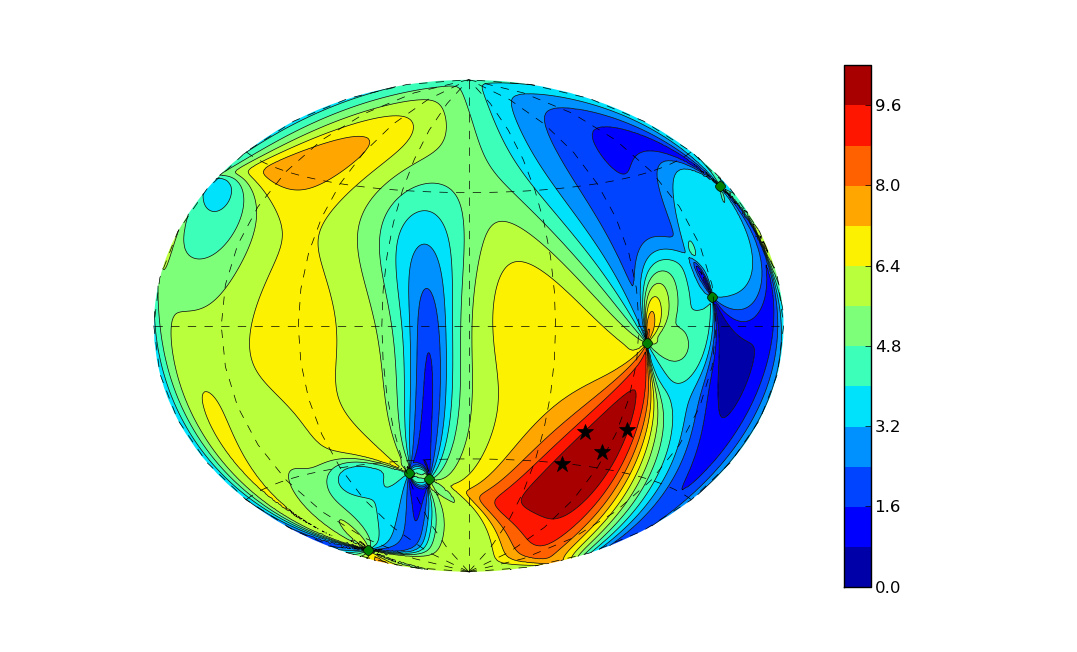
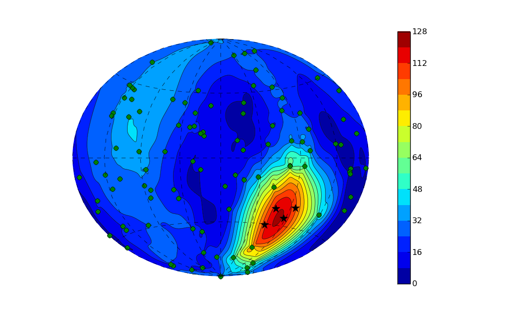
In the previous subsection we looked at the detection and sky location of one or two GW sources with variable number of pulsars. We have chosen on purpose widely separated sources. We consider now a small group (cluster) of GW sources located close to each other in the sky. The idea is to check whether we can still infer the number of sources in the cluster and resolve them individually. We consider sources of equal intrinsic strength. We start with computing the log-likelihood sky map assuming a single GW source and incrementing the number of pulsars from 6 to 100. Even with 100 pulsars the cluster looks like a single maximum in the likelihood extending over the whole cluster. The size of this maximum shrinks as we include more and more pulsars, but we do not see the development of multiple maxima corresponding to the true locations of the sources. We show likelihood contour plots in figure 5 for 6 and 100 pulsars in the array.

We then tried multiple GW source models. We started with 6 pulsars; in this case we cannot try models with more than two GW sources. The best guess for a two-source model is $\{4.60,0.90\};\{4.22,0.96\}$, to be compared to the true positions of the sources: $\{4.26,0.78\};\{4.37,0.98\};\{4.66,0.88\};\{4.82,1.01\}$. Increasing the number of pulsars to 12, we can test models with up to 4 sources. Unfortunately the result is a significant increase in the ambiguity area with poor source localization. For example, the best guess with a three source model is $\{4.84,2.03,0.0004\};\{4.28,0.88,0.123\};\{4.71,0.94,0.161\}$. The third number in each parenthesis is the estimate of the relative contribution of the source to the log-likelihood, i.e., $C_{n}$ as defined by equation (31). The first source in the solution contributes negligibly to the result: the best solution is essentially still a two-source model.

The result improves by increasing the number of pulsars and running models with 2-, 3- and 4-sources. The best guess with 100 pulsars is close to the true positions of the GW sources, and all four points give a significant contribution to the likelihood: $\{4.20,0.81,0.67\}$; $\{4.41,0.92,1.19\}$; $\{4.63,0.89,1.2281\}$; $\{4.90,1.04,0.65\}$. However the maximum likelihoods of the best 1-, 2-, 3- and 4-source solutions are very similar: 1.2144, 1.2279, 1.2281, 1.22815 (to be compared to a true likelihood of 1.22818). This means that we might not be able to differentiate between those models in practice (in presence of noise).

IV.3 Determining the number of GW sources

Figure 6: Log-likelihood sky map for the single-source model in the case of five unequal GW sources detected with an array of 50 pulsars. The true position of the five GW sources is shown as black circles, with relative size corresponding to their relative strength. Pulsars are shown as green dots.

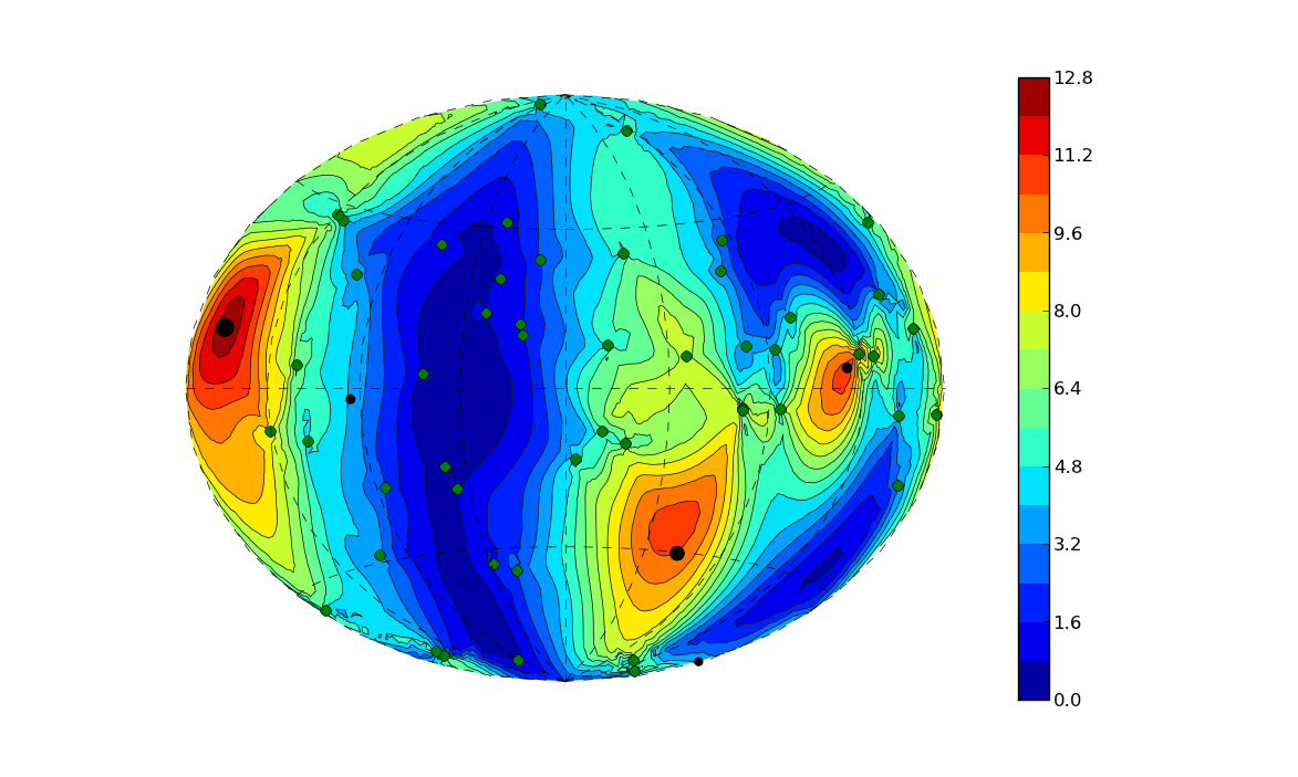
We consider now a signal generated by the superposition of five sources with known sky location and relative strength. We test two cases: in the first case, all sources have equal strength; in the second one, we take the relative source strengths of the five brightest sources found in a realization of the cosmic SMBHB population from KS11 . Sources are placed randomly in the sky, and their location is the same for both cases.

As a first test, we estimate the likelihood function of a single-source model as a function of the number $P$ of pulsars in the array. Results are similar in the two cases. In the equal strength case, when $P$ is small, we observe a single maximum resulting from the combination of the five sources. When $P\approx 30$, we detect two local maxima corresponding to the true location of two of the GW sources, and when $P\approx 50$, the local maxima correctly recover three sources. A similar situation occurs in the unequal case, with the difference that now, when $P$ is small, the single maximum corresponds to the actual position of the brightest source. Again, increasing $P$ up to 50, we observe three maxima, corresponding to the three brightest sources. The log-likelihood sky map for $P=50$ in the unequal case is shown in figure 6.

Figure 7: Maximum estimated log-likelihood of the $N$-source models as a function of $N$. The dataset contained five GW sources, and detection was performed by an array of 50 pulsars. Left panel: equal strength sources; right panel: unequal strength sources. In both cases, the maximum log-likelihood flattens out for models with more than five sources.

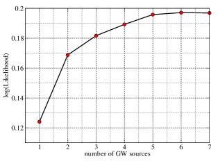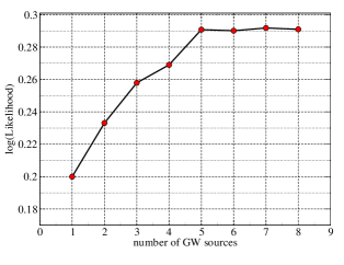
Using 50 pulsars we then tried 2-, 3-, 4-, 5-, 6-, 7-, 8-source models. We should emphasize here that our maximum likelihood search is far from being optimal, so we had to do quite extended searches for models with more than 4 GW sources. We plan to apply proper search algorithms to this problem in future work. In figure 7 we show the maximum recovered log-likelihood as a function of the number of GW sources included in the model for the two examined cases. In the equal case, we see a steady increase of the maximum likelihood up to five sources, beyond which the curve suddenly flattens out. A similar behaviour is seen in the unequal case, with the difference that now the maximum likelihood growth for 3-to-5 source models is much shallower than before. This is simply due to the unequal strength of the sources. Also in this case, the likelihood flattens out if more than five sources are included. We can therefore safely say that, at least in the limit of few sources contributing to the signal, the algorithm is capable of unambiguously identifying the number of sources present in the data.

Figure 8: Log-likelihood sky maps of the source sky positions for an injection of 5 source with equal strength, detected with an array of 50 pulsars. From the top left to the bottom right, panels show the likelihood for a 2-, 3-, 4- and 5-source model. We plot all the points which have $C_{n}$ within 10% of the maximum likelihood for each model.

Table 1: Recovered sky position of GW sources for models with different number of sources. For each model we also give the maximum likelihood estimator of the sky location $\{\phi,\theta,C_{n}\}$.

Equal strength sources
True position	2-source model	3-source model	4-source model	5-source model	6-source model	7-source model
4.262, 0.779	-	-	-	4.24, 0.57, 0.29	4.43, 1.11, 0.22	4.40, 0.72,0.24
1.496, 1.522	-	1.43, 1.46, 0.21	1.46, 1.50, 0.27	1.49, 1.53, 0.23	1.52, 1.67, 0.25	1.50, 1.52, 0.25
5.363, 1.653	5.43, 1.69, 0.17	5.38, 1.68, 0.25	5.42, 1.68, 0.22	5.30, 1.63, 0.26	5.35, 1.62, 0.25	5.27, 1.63, 0.27
6.250, 0.361	-	-	6.2, 1.03, 0.20	6.22, 0.32, 0.29	6.21, 0.42, 0.25	6.20, 0.38, 0.29
0.317, 1.794	0.57, 1.49, 0.23	0.28, 1.55, 0.26	0.37, 1.99, 0.21	0.45 1.81, 0.22	0.39, 1.86, 0.29	0.45, 1.73, 0.28
-	-	-	-	-	1.08, 1.42, 0.04	1.36, 2.17, 0.04
-	-	-	-	-	-	2.92, 1.70, 0.03
-	-	-	-	-	-	-
Unequal strength sources
True position	2-source model	3-source model	4-source model	5-source model	6-source model	7-source model
4.262, 0.779, 0.83	4.34, 086, 0.13	4.22, 0.58, 0.17	4.37, 0.61, 0.19	4.42, 0.66, 0.20	4.39, 0.70, 0.17	4.37, 0.74, 0.16
1.496, 1.522, 0.52	-	-	1.62, 1.35, 0.08	1.61, 1.55, 0.11	1.45, 1.44, 0.10	1.49, 1.41, 0.10
5.363, 1.653, 0.58	-	5.25, 1.60, 0.13	5.19, 1.70, 0.10	5.26, 1.68, 0.12	5.28, 1.65, 0.12	5.19, 1.61, 0.11
6.250, 0.361, 0.44	-	-	-	5.97, 0.39, 0.07	6.03, 0.33, 0.08	6.28, 0.30, 0.07
0.317, 1.794, 1.0	0.30, 1.73, 0.17	0.41, 1.68, 0.18	0.35, 1.65, 0.16	0.30 1.85, 0.19	0.30, 1.78, 0.20	0.34, 1.82, 0.20
-	-	-	-	-	5.09, 2.31, 0.01	3.04, 2.23, 0.01
-	-	-	-	-	-	5.64, 2.74, 0.02

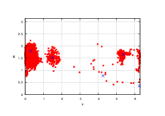
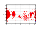
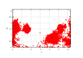
In figure 8 we try to give a sense of how the likelihood map behaves for models with more than one source. As already pointed out before, a visualization of the likelihood is not straightforward, since it is now function of $2\times N$ parameters, and is not easily represented in a 2-D plot. Here we consider the equal strength case, and we show the points giving a contribution $C_{n}$ within 10% of maximum likelihood value. In the 2-source model (upper left panel) we already clearly see three clusters around the true location of three of the injected sources. The situation does not significantly change adding a third source, but clusters around all the five sources begin to appear in the 4-source model (lower left panel) and are clearly resolved in the 5-source model (lower right panel). If we go beyond a 5-source model, the likelihood map becomes more and more diluted (increase of the ambiguity regions) without showing any significant new “cluster of points”, or any improvement of the maximum likelihood. Note that also in the 5-source model, the ambiguity areas are quite large, which would, for example, pose a serious problem to a putative search for electromagnetic counterparts to the sources sesana11 ; tanaka11 . However we have noticed that the ambiguity regions around the bright sources in the 2-source model search (see upper left panel) are notably smaller than the areas around the corresponding sources in the 5-source model search (lower right panel). We want to take this into account while constructing a proper search algorithm, by restricting the ambiguity region in the five source search to that found in the 2-3 source model. This should allow us more accurate localization of the GW sources.

As a final step, we give the best recovered source parameters for each $N$-source model in table 1. Notice that for a noiseless dataset, in principle, for a 5-source model, the best answer giving the maximum likelihood is the true one. However it might take quite a long time to converge to that answer. What we show in the table is the result of our (limited) search algorithm, which should give some ideas about the abilities to find and locate maxima. The detection strategy performs well in both cases. As $N$ increases up to 5, we recover $N$ sources almost at the right sky location. And for $N>5$, the additional sources always have a relative contribution to the likelihood which is an order of magnitude smaller than the true ones. Notice also that the recovered values of $C_{n}$, representing the relative contribution of the sources to the signal, are very close to the injected relative source strengths. In the future work we intend to apply advanced search algorithms (see, e.g., Littenberg:2009bm, ; vanderSluys:2008qx, ; Petiteau:2010zu, ; Feroz:2009de, ) developed and used for GW data analysis in present and future interferometric detectors.

V Blind searches

After testing the effectiveness of our detection strategy, we performed two sets of blind searches. For this exercise, datasets were generated by A. Sesana, and searches were performed by S. Babak without any previous knowledge of the content of the datasets, except for the fact that there were less than 10 sources.

V.1 Noiseless data

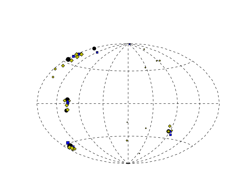
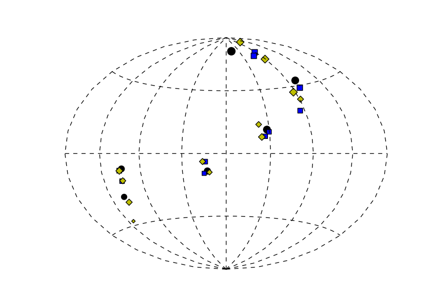
In the first round of blind searches, we used noiseless datasets. We used equally sampled (once every two weeks) time series for 50 pulsars located randomly in the sky. Two datasets were analyzed, both of them containing six sources with unequal strengths at a frequency $f=2\times 10^{-8}$Hz. The first search inferred 5 or 7 sources (corresponding to maximum likelihoods of 0.131 and 0.133, to be compared with 0.1345 which is the likelihood for the actual position of the 6 injected sources). In the second blind search the best guesses were 5 or 6 sources with maximum likelihood of 0.0699 and 0.071 respectively (to be compared to 0.077 for the true injection). In the first dataset there were two close pairs of sources, while in the second one there was only one tight pair. The presence of tight pairs makes the source recovery problematic, especially because we do not use any optimized search algorithm (note that in both cases, the maximum estimated likelihood is quite smaller than the true one). Results are visualized in figure  9. Here, filled black circles denote the true location of the GW sources, and coloured diamonds and squares correspond to points extracted by the best model solutions. The relative size of the symbols represent either the relative strength of the sources, or the relative contribution to the likelihood of the recovered points. Isolated sources are clearly identified, and their inferred position is usually within few degrees of the true one. Close pairs are more problematic, because sometimes the search algorithm recognize a single source, midway between the two. We expect these results to improve in a optimized search.

Figure 9: Results of the noiseless blind searches. Left panel: few points from the best 5-source (blue) and 7-source (yellow) solutions for the first dataset. Right plot: best guesses from the 5-source model (blue) and from the 6-source model (yellow). The relative size of the symbols indicates the relative contribution of each point to the combined likelihood. In both panels, the injected sources are shown as filled circles, with relative size corresponding to their relative strength.

V.2 Noisy data

We finally tackled a more ‘realistic’ situation in which white noise was added to the data (note that the spectral properties of the noise is irrelevant here, since we perform a ‘monochromatic’ exercise). We considered two situation representative of realistic scenarios that might be realized in the near future:

1. Hard search: 30 pulsars with equal rms noise of 100ns, which is the nominal sensitivity goal of the IPTA collaboration hobbs2010 ;

2. Easy search: 50 pulsars with equal rms noise of 30ns, which is what it might (conservatively) be achieved with the SKA.

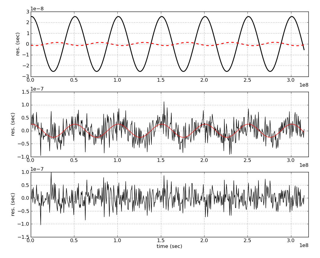
Both datasets were again equally sampled once every two weeks over a timespan of 10 years, and few sources with unequal strength of the order of $50-100$ns (consistent with the strongest sources predicted by state of the art SMBHB population models) were injected at a frequency $f=2\times 10^{-8}$Hz. An example of ‘easy’ data stream is shown in figure 10. The signal is clearly visible by eye in the noisy data (middle panel). In the ‘easy’ search, SNRs in each single pulsars were in fact between 5 and 30, with total SNR in the array of $162.33$. In the ‘hard’ case, SNRs in some individual pulsars were even $<1$, with a total SNR in the array of $23.65$.

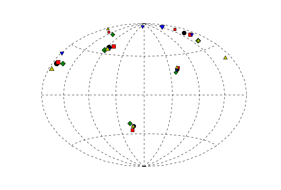
Results for the ‘easy’ search are shown in the left panel of figure 11, where the four best solutions are plotted. All the solutions inferred 5-to-7 sources, pinning down the position of most of the injections within just a few degrees. In particular, the seven-source solution showed with red squares recovered correctly all the five sources within $<10$ degrees of their true location, whereas the two additional sources inferred by the solution contribute much less (factor of two-to-three) to the likelihood of the solution with respect to the other five. A good performance was expected in this case, since the SNR is so high that we are approaching the noiseless limit.

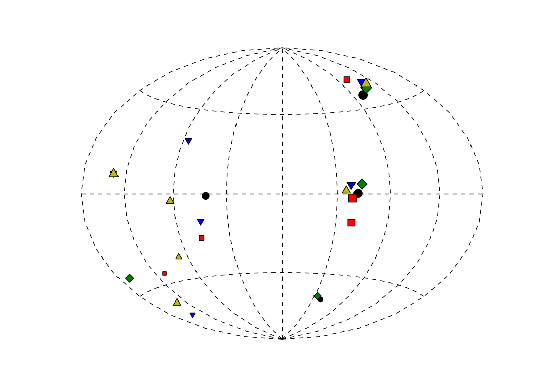
The four best solutions to the ‘hard’ search are shown in the right panel of figure 11. Here we see a different situation: all the solutions correctly recover the two brightest sources within few degrees of their true location. However the weakest two are often missing or misidentified. Four-five source solutions are clearly preferred (higher maximum likelihood), but the weakest sources are not correctly recovered. This is simply because their SNR in the array ( $\sim 4.5$ and $\sim 10.1$) is both small in absolute terms, and relative to the brighter sources (SNR $\sim 13.7$ and $\sim 15.9$). The noise contribution is rather significant in this case, as it creates additional (to the noiseless, intrinsic) ambiguity by promoting secondary likelihood maxima. By inspecting individual datasets as the one shown in figure 10, we noticed that no more than 10-15 pulsars significantly contribute to the total SNR in the array, being the SNR in the others of order unity. This means that we effectively have barely enough pulsars to estimate all the parameters of the four sources, which might also contribute to the difficulties of locating the weaker sources in the sky. We expect a proper search to improve these results.

Figure 10: Example of residuals used in the blind search. The dataset contained a superposition of five monochromatic sources at $f=2\times 10^{-8}$Hz, shown as a black line in the upper panel. The central panel shows an example of dataset (black line) made of a Gaussian white noise with $\sigma=30$ns plus the injected signal (red line). The lower panel show the residual noise after the best estimate of the signal was removed. The residual signal after removal of the best estimate is shown as a red–dashed line in the upper panel.

Figure 11: Results of the blind search with noise. Left panel: ’easy search’; filled–black circles represent the injected sources, whereas each set of colored symbols represents a ’high likelihood’ solution of the blind search. Right panel: same as the left panel but for the ’hard search’. The size of the black dots is proportional to the injected source strength; the size of the colored symbols is proportional to their contribution to the likelihood.

VI Discussion

We have investigated for the first time the possibility of exploiting the information enclosed in the spatial distribution of a pulsar timing array to resolve gravitational wave sources individually. To this purpose, we employ a maximum likelihood-based algorithm and tested its performance in a number of simple, idealized situations. Under the simplifications and assumptions listed in the Section II, we can draw the following conclusions:

• to estimate the sky location of all $N$ GW source we need at least $P=3\times N$ pulsars;

• if $P<3\times N$ we can still make reliable estimations of the position of some (usually the strongest) GW sources;

• in this latter case, removing the stronger sources from the solution, also removes power belonging to the weaker ones, causing their misidentification or misplacement;

• it is beneficial to run low $N$-source models even if we know that there are many more sources. Our results show that such low $N$-source models usually allow detection and correct sky location of the brightest GW sources;

• computation of the likelihood with increasingly number of sources assumed in the model resolves more GW sources but at the same time increases the ambiguity (error) regions;

• if the GW sources are located close to each other in the sky, they cannot be reliably resolved individually, and appear as a single large ambiguity region. However, the maximum likelihood estimator usually favors multi source models, giving valuable information on the number of sources present in the cluster;

• in the limit of low number $N$ of GW sources, the maximum likelihood estimator allows to infer the correct number of sources present in the datasets (as long as $P>3\times N$). In the noiseless case, even by using very primitive search techniques, we are able to correctly identify and locate all the sources in the sky within few degrees of their true location;

• in presence of noise, we can also infer the correct number of sources and locate the bright ones in the sky. The presence of dimmer sources can be correctly inferred, but due to their low SNR they are easily misplaced.

This study mostly represents a proof of concept of the possibility of utilizing the spatial information enclosed in the array to disentangle signals that would otherwise appear like a confusion foreground. In particular, most of the results were derived in the noiseless limit. On the other hand, the employed search methods were very simple and largely non-optimal, which somehow limited the capabilities of the analysis. In future investigations, we plan to expand our analysis in several ways to assess its full potential in more realistic scenarios. In particular we will:

1. test the limit of large number of sources, where $N\gg P$;

2. draw the source strength distribution from state of the art models of the cosmological population of SMBHBs;

3. include the pulsar terms in the signal and perform frequency searches;

4. consider different noise levels and noise spectra in each single pulsar in the array;

5. optimize the effectiveness of our analysis technique by employing proper multimodal search algorithms, similar to those applied in Petiteau:2010zu ; Feroz:2009de .

Pulsar timing arrays will be powerful gravitational wave detectors, and further studies along the line of the present investigation will help exploiting their full potential as astrophysical observatories.

References

- (1) M. V. Sazhin, Soviet Astronomy 22, 36 (1978).
- (2) R. W. Hellings and G. S. Downs, Astrophys. J. Lett. 265, L39 (1983).
- (3) R. N. Manchester, The Parkes Pulsar Timing Array Project, in 40 Years of Pulsars: Millisecond Pulsars, Magnetars and More, edited by C. Bassa, Z. Wang, A. Cumming, & V. M. Kaspi, , American Institute of Physics Conference Series Vol. 983, pp. 584–592, 2008, [0710.5026].
- (4) G. H. Janssen et al., European Pulsar Timing Array, in 40 Years of Pulsars: Millisecond Pulsars, Magnetars and More, edited by C. Bassa, Z. Wang, A. Cumming, & V. M. Kaspi, , American Institute of Physics Conference Series Vol. 983, pp. 633–635, 2008.
- (5) e. a. Jenet, ArXiv e-prints 0909.1058 (2009), [0909.1058].
- (6) e. a. Hobbs, G., Classical and Quantum Gravity 27, 084013 (2010), [0911.5206].
- (7) R. Smits et al., Astronomy & Astrophysics 505, 919 (2009), [0908.1689].
- (8) J. Lazio, The Square Kilometre Array, in Panoramic Radio Astronomy: Wide-field 1-2 GHz Research on Galaxy Evolution, 2009, [0910.0632].
- (9) G. Nelemans, L. R. Yungelson and S. F. Portegies Zwart, Astronomy & Astrophysics 375, 890 (2001), [arXiv:astro-ph/0105221].
- (10) M. Rajagopal and R. W. Romani, Astrophys. J. 446, 543 (1995), [arXiv:astro-ph/9412038].
- (11) A. H. Jaffe and D. C. Backer, Astrophys. J. 583, 616 (2003), [arXiv:astro-ph/0210148].
- (12) A. Sesana, A. Vecchio and C. N. Colacino, Mon. Not. R. Astron. Soc. 390, 192 (2008), [0804.4476].
- (13) A. Sesana, A. Vecchio and M. Volonteri, Mon. Not. R. Astron. Soc. 394, 2255 (2009), [0809.3412].
- (14) F. A. Jenet, G. B. Hobbs, K. J. Lee and R. N. Manchester, Astrophys. J. Letter 625, L123 (2005), [arXiv:astro-ph/0504458].
- (15) F. A. Jenet et al., Astrophys. J. 653, 1571 (2006), [arXiv:astro-ph/0609013].
- (16) M. Anholm, S. Ballmer, J. D. E. Creighton, L. R. Price and X. Siemens, Phys. Rev. D 79, 084030 (2009), [0809.0701].
- (17) R. van Haasteren, Y. Levin, P. McDonald and T. Lu, Mon. Not. R. Astron. Soc. 395, 1005 (2009), [0809.0791].
- (18) v. et al., Mon. Not. R. Astron. Soc. 414, 3117 (2011), [1103.0576].
- (19) F. A. Jenet, A. Lommen, S. L. Larson and L. Wen, Astrophys. J. 606, 799 (2004), [arXiv:astro-ph/0310276].
- (20) A. Sesana and A. Vecchio, Phys. Rev. D 81, 104008 (2010), [1003.0677].
- (21) V. Corbin and N. J. Cornish, ArXiv e-prints 1008.1782 (2010), [1008.1782].
- (22) D. R. B. Yardley et al., Mon. Not. R. Astron. Soc. 407, 669 (2010), [1005.1667].
- (23) K. J. Lee et al., Mon. Not. R. Astron. Soc. 414, 3251 (2011), [1103.0115].
- (24) B. Kocsis and A. Sesana, Mon. Not. R. Astron. Soc. 411, 1467 (2011), [1002.0584].
- (25) L. Boyle and U.-L. Pen, ArXiv e-prints (2010), [1010.4337].
- (26) P. Jaranowski, A. Królak and B. F. Schutz, Phys. Rev. D 58, 063001 (1998), [arXiv:gr-qc/9804014].
- (27) A. Vecchio, Phys. Rev. D 70, 042001 (2004), [arXiv:astro-ph/0304051].
- (28) A. Sesana, C. Roedig, M. T. Reynolds and M. Dotti, ArXiv e-prints (2011), [1107.2927].
- (29) T. Tanaka, K. Menou and Z. Haiman, ArXiv e-prints (2011), [1107.2937].
- (30) T. B. Littenberg and N. J. Cornish, Phys. Rev. D80, 063007 (2009), [0902.0368].
- (31) M. van der Sluys et al., Class. Quant. Grav. 25, 184011 (2008), [0805.1689].
- (32) A. Petiteau, Y. Shang, S. Babak and F. Feroz, Phys. Rev. D81, 104016 (2010), [1001.5380].
- (33) F. Feroz, J. R. Gair, M. P. Hobson and E. K. Porter, Class. Quant. Grav. 26, 215003 (2009), [0904.1544].