Mechanism for puddle formation in graphene

Abstract

When graphene is close to charge neutrality, its energy landscape is highly inhomogeneous, forming a sea of electron-like and hole-like puddles, which determine the properties of graphene at low carrier density. However, the details of the puddle formation have remained elusive. We demonstrate numerically that in sharp contrast to monolayer graphene, the normalized autocorrelation function for the puddle landscape in bilayer graphene depends only on the distance between the graphene and the source of the long-ranged impurity potential. By comparing with available experimental data, we find quantitative evidence for the implied differences in scanning tunneling microscopy measurements of electron and hole puddles for monolayer and bilayer graphene in nominally the same disorder potential.

I Introduction

In monolayer graphene, the hexagonal arrangement of carbon atoms dictates that in the absence of atomic-scale disorder, graphene is a gapless semiconductorDas Sarma et al. (2011); Castro Neto et al. (2009) that is always metallic at low temperature.Fuhrer and Adam (2009) This metallic behavior holds even in the presence of quantum interference and strong disorder,Bardarson et al. (2007) in stark contrast to most other materials, which undergo a metal-to-insulator transition at low carrier density.Anderson (1958); Tanatar and Ceperley (1989) The physical origin for this robust metallic state is that the ground-state of graphene at vanishing mean carrier density becomes spatially inhomogeneous, breaking up into electron-rich and hole-rich metallic regions connected by highly conducting p-n junctions.Katsnelson et al. (2006) Bilayer graphene comprising two sheets of graphene that become strongly coupled due to the $AB$ stacking arrangementMcCann and Fal’ko (2006) shares some properties with regular semiconductors (such as the parabolic band dispersion) and in other ways behaves like monolayer graphene, including having chiral wavefunctions and forming electron and hole puddles at low density.

These electron and hole puddles have now been observed in several experiments of exfoliated graphene on an insulating SiO₂ substrate including Refs. Martin et al., 2008; Zhang et al., 2009; Deshpande et al., 2009, 2011; Jung et al., 2011; Rutter et al., 2011. While these authors suggest that long-range charged impurities in the substrate could be responsible for the spatial inhomogeneity, detailed comparisons to microscopic models have not been made.

In this paper, we demonstrate that differences between the spatial properties of puddles in monolayer and bilayer graphene can be quantitatively explained by the differences in the screening properties of the two systems (that ultimately arises from the differences in their band-structure). Numerical results show that the correlation length for bilayer graphene is relatively independent of density and significantly smaller than that of monolayer graphene for a typical range of impurity densities. Finally, we find good quantitative agreement when comparing our results with available experimental data.

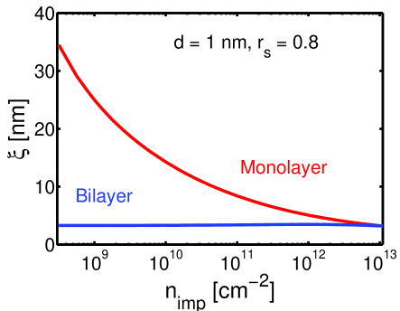
The rest of the paper is organized as follows. In Sec. II, we outline the the theoretical model, providing a heuristic understanding of our results using the Thomas-Fermi (TF) screening theory. However, the TF significantly underestimates the effect of electronic screening in both monolayer and bilayer graphene. It is therefore necessary to use the Random Phase Approximation (RPA) screening theory, which we discuss in Sec. III. Our main finding is that the puddle correlation length in bilayer graphene $(\xi\approx 3.5~{}{\rm nm})$ is relatively insensitive to the impurity concentration and carrier doping. This is in contrast to monolayer graphene, where the puddle correlation length varies from $3~{}{\rm nm}$ in dirty samples to more than $35~{}{\rm nm}$ in clean samples.

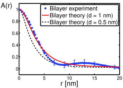
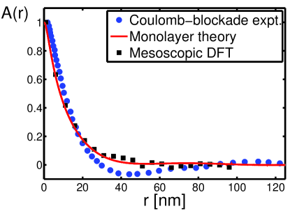
The comparison with experiment is done in Sec. IV, where we examine three different experimental results: (1) We consider first the experimentally determined normalized correlation function $A(r)$ (see definition below) obtained from the scanning tunneling microscopy (STM) data reported for exfoliated bilayer graphene in Ref. Rutter et al., 2011. The full functional form of $A(r)$ agrees with the theory where the only adjusted parameter in the theory is the distance $d$ of the impurities from the graphene sheet. In particular the experimentally determined correlation length $\xi=(3.68\pm 0.03)~{}{\rm nm}$, defined here as the half-width at half-maximum (HWHM) decay length of $A(r)$ agrees well with the $d=1~{}{\rm nm}$ RPA theory value of $\xi=3.4~{}{\rm nm}$. This value of $d$ is both reasonable and consistent with those determined from other transport measurements on bilayer graphene.Adam and Das Sarma (2008) (2) From the monolayer graphene STM experimental data reported in Ref. Jung et al., 2011, we extract a correlation length $6~{}{\rm nm}<\xi<11~{}{\rm nm}$. Since the measurements Jung et al. (2011); Rutter et al. (2011) were made on the same exfoliated graphene sample containing both single layer and bilayer graphene regions, we expect that the extrinsic disorder potential is statistically identical for the two samples. Therefore, using the value of $d=1~{}{\rm nm}$ (discussed above) and the disorder induced Dirac point shift reported in Ref. Rutter et al., 2011, we calculate theoretically (without any adjustable parameters) that a monolayer graphene sample in the same disorder environment would have a puddle correlation length $\xi=8~{}{\rm nm}$, in reasonable agreement with the experiment. (3) We then compare $A(r)$ obtained using scanning Coulomb blockade spectroscopy reported in Ref. Deshpande et al., 2011 with our theoretical results for monolayer graphene at the Dirac point. The parameters used in the theory were obtained from separate transport measurements on the same experimental sample.Deshpande et al. (2011) The agreement between theory and experiment is remarkable since it involves no adjustable parameters. Finally in Sec. V, we conclude by making predictions for future experiments involving monolayer and bilayer graphene on BN substrates.

II Formalism

The doping level of graphene can be measured in a variety of different ways. In transport measurements, the gate voltage potential that yields the resistivity maximum identifies the extrinsic doping level due to extraneous sources, such as charged impurities in the substrate impurities with density, $n_{imp}$. While the width of the resistivity maximum is a measure of the homogeneity of the sample, Adam et al. (2007) or the electron-hole puddle distribution.

In local probe measurements, such as STM, the Dirac point energy relative to the Fermi-level can be observed as a minimum in the tunneling differential conductance, $dI/dV$ as a function of tunneling bias. Knowing the electronic dispersion relation (see details below), for a particular gate voltage $V_{g}$, this spatial map $V(r)$ of the Dirac point variation can then be used to extract the spatial distribution of the local carrier density (characterized by a width $n_{\rm rms}$). We can also characterize the puddles through the radially averaged autocorrelation function

$$C(r)=\frac{1}{2\pi}\int\limits_{0}^{2\pi}d\phi\langle\langle V({\bf r})V(0)\rangle\rangle,$$ (1)

where the angular brackets denote an average over the image area and the $\phi$-integration averages over orientations.

Notice that while $C(0)=V_{\rm rms}^{2}$ (which is related to $n_{\rm rms}$) characterizes the fluctuations in the puddle depth, $C(r)$ describes the spatial profile of the electron and hole puddles. We find it useful to consider the normalized correlation function $A(r)=C(r)/C(0)$. We will argue below that $A(r)$ and $C(0)$ are quite different physical quantities that depends quite differently on the parameters of the extrinsic impurity potential. (In addition, for a typical STM experiment, where the shifts in the Dirac point are determined Zhang et al. (2009) from the shifts in $dI/dV$ at fixed $V_{g}$, the determination of $C(0)$ is complicated by the experimental uncertainty in converting spatial maps of $dI/dV$ to Dirac point energy shifts $V({\bf r})$. By contrast, the much smaller uncertainty in $A(r)$ is mostly determined by the spatial resolution and image area.)

To theoretically compute the correlation functions for puddles in graphene, we make two assumptions. First, the impurity potential comes from a random two dimensional distribution of charged impurities displaced by a distance $d$ from the plane with density $n_{\rm imp}$. This model has been highly successful in describing the effect of disorder in semiconductor heterojunctionsAndo et al. (1982) and in graphene.Das Sarma et al. (2011) This spatially varying potential gives rise to a varying charge density and local variations in the screening of the potential. Second, we assume that it is possible to find a global screening function $\epsilon(q,n_{\rm eff})$ that adequately describes the effects of these local screening variations. Here, the screening depends on the disorder potential only through an effective carrier density $n_{\rm eff}$. This self-consistent screening model has been used previously to understand the minimum conductivity problem in both monolayerAdam et al. (2007) and bilayer graphene.Adam and Das Sarma (2008) If these two assumptions are satisfied, the correlation function, aside from a prefactor of $n_{\rm imp}$, then depends only on the screened impurity potential

$$C(r) = 2\pi n_{\rm imp}\left(\frac{e^{2}}{\kappa}\right)^{2}\int_{0}^{\infty}dq\frac{q\exp(-2qd)}{[q\epsilon(q,n_{\rm eff})]^{2}}J_{0}(qr),$$ (2)

where $\kappa$ is the bulk (3D) dielectric constant, $\epsilon(q)$ is the surface (2D) screening function in the plane, $-e$ the electron charge, and $J_{0}(x)$ is a Bessel function.

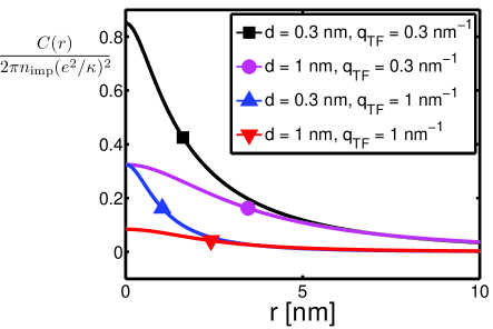
As an illustration, consider the Thomas-Fermi (TF) screening for which the surface dielectric function is given by $\epsilon(q,n_{\rm eff})=1+q_{\rm TF}(n_{\rm eff})/q$, where $q_{\rm TF}(n_{\rm eff})$ (discussed below) is the Thomas-Fermi screening wavevector. Shown in Fig. 1 is a calculation of $C(r)$ for different values of $q_{\rm TF}$ and $d$. Notice that for fixed $q_{\rm TF}$, the spatial dependence of $C(r)$ depends on $d$ and $q_{\rm TF}$, but not on $n_{\rm imp}$. On the other-hand, the function $C(0)$ (which, within the TF can be calculated analytically) depends on $n_{\rm imp}$, $\kappa$, $d$ and $q_{\rm TF}$. This is why we find it useful to use the normalized correlation function $A(r)=C(r)/C(0)$ that describes the spatial profile of the screened impurity potential. We also emphasize that $A(r)$ contains different information than the typical puddle size – for example, the puddle correlation length $\xi$ (recall that $\xi$ is defined as the HWHM of $A(r)$) describes the width of the screened impurity potential, and not the mean impurity separation. For example, in the low impurity density limit, spatial maps of the puddles would show isolated impurities, but $A(r)$ would not change (for fixed $q_{\rm TF}$). Moreover, since $A(r)$ scales differently with $q_{\rm TF}$ and $d$, in principle, both of these length scales can be extracted from a measurement of $A(r)$.

Figure 1: Theoretical calculations for the correlation function $C(r)$ using the Thomas-Fermi approximation. This autocorrelation function depends separately on the typical distance $d$ of long-ranged impurities from the graphene sheet, and $q_{\rm TF}$ the inverse effective screening length, allowing them to be determined independently. Symbols show the correlation length $\xi$, defined as the HWHM length.

Within the TF screening theory, any differences between monolayer and bilayer graphene can only arise from differences in $q_{\rm TF}(n_{\rm eff})$. The linear dispersion in monolayer graphene and the hyperbolic dispersion in bilayer graphene gives rise to these differences. The low energy linearly dispersing bands of monolayer graphene can be modeled by a single parameter, the Fermi velocity $v_{\rm F}$, or equivalently, the effective fine-structure constant $r_{s}=e^{2}/(\kappa\hbar v_{\rm F})\approx 0.8$. $r_{s}$ characterizes the strength of the electron-electron interaction for graphene on a SiO₂ substrateDas Sarma et al. (2011) and is useful because we are interested in the screening properties of graphene. The Thomas-Fermi screening wavevector is related to the density of states, and for monolayer graphene is given by $q_{\rm TF}(n_{\rm eff})=4r_{s}\sqrt{\pi n_{\rm eff}}$, where $n_{\rm eff}$ is the effective carrier density.

Bilayer graphene can be modeled with a hyperbolic dispersion with two parameters $v_{\rm F}$ (throughout this manuscript, $v_{\rm F}$ is the Fermi velocity of a single decoupled graphene sheet), and the low-energy effective mass $m_{\rm eff}$. For simplicity we use for the two parameters $r_{s}$ (defined above) and $n_{0}=m_{\rm eff}^{2}v_{\rm F}^{2}/(\hbar^{2}\pi)\approx 2.3\times 10^{12}~{}{\rm cm}^{-2}$ which is the characteristic density scale for the crossover from a (low density) parabolic to a (high density) linear dispersion. The Thomas-Fermi screening wavevector for bilayer graphene is given by $q_{\rm TF}(n_{\rm eff})=4r_{s}\sqrt{\pi n_{0}}\sqrt{1+n_{\rm eff}/n_{0}}$.

As the system approaches the Dirac point, the fluctuations in carrier density become larger than the average density. In this case, screening varies spatially with the density fluctuations. We assume that it is possible to describe the effect of this screening by using the screening for an ideal system and an effective carrier density $n_{\rm eff}$ obtained self-consistently.Adam et al. (2007) This is done by equating the squared Fermi level shift with respect to the Dirac point with the square of the potential fluctuations, $E^{2}[n=n_{\rm eff}]=C(0)$ where $C(0)$ is defined in Eq. 2 and $E[n]=\hbar v_{\rm F}\sqrt{\pi n}$ for monolayer graphene, and $E[n]=v_{\rm F}^{2}m_{\rm eff}\left[\sqrt{1+n/n_{0}}-1\right]$ for bilayer graphene. The result of this procedure are shown in Fig. 2.

Figure 2: Effective carrier density as a function of impurity density assuming $d=1~{}{\rm nm}$, $r_{s}=0.8$, and $n_{0}=2.3\times 10^{12}~{}{\rm cm}^{-2}$. For bilayer graphene, the blue circles show the Thomas-Fermi approximation and the red squares are RPA results. The empirical relation $n_{\rm eff}=\sqrt{n_{\rm imp}~{}n_{1}}$ adequately captures the RPA results, with $n_{1}=6.8\times 10^{11}~{}{\rm cm}^{-2}$.

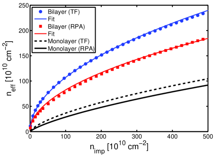
Within the TF theory, we can now qualitatively discuss the main differences between monolayer and bilayer graphene. For bilayer graphene, the inverse screening length changes only slightly from the low density value of $q_{\rm BLG}\approx 4r_{s}\sqrt{\pi n_{0}}$ that is set entirely by the band parameters. As a consequence, the puddle correlation length does not change with the impurity concentration or carrier density, and depends only on the distance $d$ of the bilayer graphene sheet from the source of the long-ranged impurity potential. In contrast, for monolayer graphene, $q_{\rm MLG}=4r_{s}\sqrt{\pi n_{\rm eff}}$ depends essentially on $C(0)$ (and therefore on $n_{\rm imp}$). This heuristic description (which we make more quantitative below) implies that depending on the sample quality, choice of substrate, or doping, the puddle correlation length in monolayer graphene (but not bilayer graphene) could vary by more than an order of magnitude.

III Random Phase Approximation

While the TF screening theory discussed in the previous section is useful to obtain a qualitative picture, we find that it significantly underestimates the effect of electronic screening. In both monolayer and bilayer graphene it gives larger values for $C(0)$ and smaller values for $\xi$. In what follows we use the the random phase approximation (RPA) where the screening function is obtained using $\epsilon(q)=1+q_{\rm TF}{\tilde{\Pi}}(q)/q$.

The normalized polarizability ${\tilde{\Pi}}(q)$ for monolayerHwang and Das Sarma (2007) and bilayerGamayun (2011) graphene are both available in the literature. We note that for monolayer graphene ${\tilde{\Pi}}(q)$ depends only on the dimensionless variable $x=q/(2\sqrt{\pi n_{\rm eff}})$

$${\tilde{\Pi}}(x) = 1+\theta(x-1)\left[\frac{\pi x}{4}-\frac{x}{2}{\rm arccsc}(x)-\frac{\sqrt{1-x^{-2}}}{2}\right],$$ (3)

$$\approx \theta(1-x)+\theta(x-1)\frac{\pi x}{4},$$

where $\theta(x)$ is a step-function and $D_{0}$ is the density of states with $q_{\rm TF}=2\pi(e^{2}/\kappa)D_{0}=4\sqrt{\pi n_{\rm eff}}r_{s}$.

In contrast, for bilayer graphene, the polarizability depends both on the scaled momentum transfer $x$, and on $\eta=n_{\rm eff}/n_{0}<8$, which parameterizes the bilayer hyperbolic dispersion relation. For $\eta\ll 1$, the bilayer graphene dispersion is quadratic, while for $1\ll\eta\leq 8$, the dispersion is linear. For $\eta>8$, one must consider the effects of a second higher-energy band that provides additional screeningMin et al. (2011) and is not considered here. By restricting the density to $n\leq 8n_{0}$, we can simplify the expression for the bilayer polarizability reported in Ref. Gamayun, 2011. Using the bilayer density of states $D=D_{0}\sqrt{1+\eta}$, with $D_{0}=2m/(\pi\hbar^{2})$, the normalized polarizability function ${\tilde{\Pi}}(x,\eta)=\Pi(q)/D_{0}$ is given by

$${\tilde{\Pi}}(x,\eta) = f(x,\eta)+\theta(x-1)g(x,\eta),$$

$$f(x,\eta) = \left[1-x^{2}\eta+x^{4}(2+\eta+2\sqrt{1+\eta})\right]^{1/2}-\ln\left[\frac{2\sqrt{1+\eta x^{2}}}{-1+\sqrt{1+\eta}}\right]-\frac{1}{2}+\frac{3x^{2}\eta-1}{2x\sqrt{\eta}}\arctan(x\sqrt{\eta})$$

$$\mbox{}+\sqrt{1-x^{2}\eta}\left(2{\rm arctanh}(\sqrt{1-\eta x^{2}})-{\rm arcsinh}\left[\frac{\sqrt{1-x^{2}\eta}(-1+\sqrt{1+\eta})}{x^{2}\eta}\right]\right)+\sqrt{1+\eta}$$

$$g(x,\eta) = \frac{-\sqrt{x^{2}-1}(1+\eta+2x^{2}\eta-\sqrt{1+\eta})}{2x(\sqrt{1+\eta}-1)}+\frac{(3x^{2}\eta-1)}{2x\sqrt{\eta}}\arccos\left[\sqrt{\frac{1+\eta}{1+x^{2}\eta}}\right]$$ (4)

$$\mbox{}+{\rm arctanh}\left[\frac{x\sqrt{x^{2}-1}\eta}{1+x^{2}\eta-\sqrt{1+\eta}}\right].$$

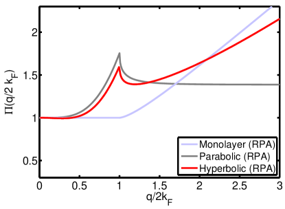
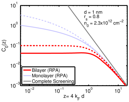
The polarizability functions for monolayer and bilayer graphene are shown in Fig. 3. What is left is to calculate the effective residual density $n_{\rm eff}$ as a function of impurity concentration. As discussed earlier, this is obtained by first calculating the autocorrelation function $C(0)$ from Eq. 2, using the RPA results shown in Fig. 3. Figure 4 shows the autocorrelation function $C(0)$ obtained using the RPA results (solid lines) as well the Thomas-Fermi results (dashed lines). We note that except at very high density (where both monolayer and bilayer graphene approach the “complete screening” limit, with $C(0)=(4k_{\rm F}r_{s}d)^{-2}$), the Thomas-Fermi approximation grossly underestimates the effect of screening. Moreover, for typical densities in bilayer graphene $C(0)$ is approximately constant and independent of carrier density consistent with the heuristic picture discussed at the end of Sec. II.

Figure 3: The Random Phase Approximation polarizability function $\Pi(q)$ normalized by the density of states for monolayer graphene and for bilayer graphene with a hyperbolic dispersion. Also shown is the parabolic approximation for the bilayer, which can be obtained from the hyperbolic dispersion when $\eta\ll 1$. The Thomas-Fermi approximation discussed in the text corresponds to the assumption that the normalized $\Pi(q)=1$ for all $q$.

Figure 4: Potential autocorrelation function $C[0]$ for monolayer and bilayer graphene. At the Dirac point, $k_{\rm F}$ is the Fermi wavevector arising from the effective carrier density i.e. $k_{\rm F}=\sqrt{\pi n_{\rm eff}}$. For large density $4k_{\rm F}r_{s}d\gg 1$, both the monolayer and bilayer results approach the “complete screening” limit, defined here as $C(0)=(4k_{\rm F}r_{s}d)^{-2}$. Notice that the Thomas-Fermi approximation shown as dashed lines captures the correct qualitative behavior, but can give significantly larger values for $C[0]$, and is therefore unsuitable for quantitative comparisons.

The effective density calculated within the RPA is shown in Fig. 2. For bilayer graphene, we find that the following empirical relationship adequately describes the numerical results

$$n_{\rm eff}=\sqrt{n_{\rm imp}~{}n_{1}},$$ (5)

where $n_{1}=11.5\times 10^{11}~{}{\rm cm}^{-2}$ for the Thomas-Fermi approximation, and $n_{1}=6.8\times 10^{11}~{}{\rm cm}^{-2}$ for the RPA results. The scaling of the bilayer effective density $n_{\rm eff}\sim\sqrt{n_{\rm imp}}$ can be anticipated for the TF approximation in the limit $n_{\rm eff}\ll n_{0}$. However, it is surprising that the simple empirical relation continues to hold both for the RPA screening theory, and for larger values of $n_{\rm eff}$.

This dependence of $n_{\rm eff}\sim\sqrt{n_{\rm imp}}$ for bilayer graphene should be contrasted with similar results obtained previously for monolayer graphene,Adam et al. (2007) where $n_{\rm eff}=2r_{s}^{2}C[0]n_{\rm imp}$ cannot be captured by a similar empirical fit. For comparison, these earlier results are also shown in Fig. 2, where we emphasize that for a given impurity concentration ($n_{\rm imp}$), bilayer graphene exhibits larger density fluctuations ($n_{\rm eff}$) than monolayer graphene. Finally, using Eq. 2, we can also calculate the puddle correlation function, and the corresponding HWHM correlation length, $\xi$, that is shown in Fig. 5

Figure 5: Theoretical results for the puddle correlation length at the Dirac point as a function of impurity concentration. While the puddle size in bilayer graphene ($\xi\approx 3.5~{}{\rm nm}$) is relatively insensitive to the disorder concentration, the size of the puddles in monolayer graphene varies from $3~{}{\rm nm}$ in dirty samples to more than $35~{}{\rm nm}$ in clean samples.

IV Comparison With Experiments

We now compare the calculated correlation functions with experiment. Figure  6(a) shows that for bilayer graphene, $A(r)$ extracted from the data reported in Ref. Rutter et al., 2011 agrees with the calculation for $d=1~{}{\rm nm}$.kn: (a) The circles show the experimental data and the RPA theory for bilayer graphene is shown for $d=1~{}{\rm nm}$ (solid curve) and $d=0.5~{}{\rm nm}$ (dashed curve). The theoretical results are insensitive to the impurity concentration $n_{\rm imp}$ and to how far the doping is away from the Dirac point. Consequently, the only free parameter in the theory is the distance $d$ of the impurities from the graphene sheet.

Figure 6: Comparison of theoretical results with experimental data. Top panel shows the normalized correlation function $A(r)=C(r)/C(0)$ for bilayer graphene. The circles are from the experimental data and solid curve is the theory for bilayer graphene with $d=1~{}{\rm nm}$. The theory curve is insensitive to impurity concentration and doping away from the Dirac point. The error bars indicate single standard deviation uncertainties.kn: (a) The small oscillation in the data over the monotonic decrease is a result of the finite size of the experimental image. Bottom panel is the normalized puddle correlation function in monolayer graphene at the Dirac point. Note the change in $x$-axis scale from bilayer graphene in top panel. The solid curve is obtained from the self-consistent screening theory. The black squares are the results of a numerical mesoscopic density functional theory calculation for the ground-state properties of monolayer graphene,Rossi and Das Sarma (2008) while the circles are experimental data taken from Deshpande et al.(Ref. Deshpande et al., 2011). Transport measurements on that same device set $n_{\rm imp}=10^{11}{\rm cm}^{-2}$ which is the value used for the theory curves. The theory also uses $d=1~{}{\rm nm}$, which is the typical distance of the impurities from the graphene sheet extracted from transport measurements of graphene on SiO₂.Tan et al. (2007)

In Ref. Rutter et al., 2011, we reported a maximum peak-to-peak carrier density fluctuation of $3.6\times 10^{11}~{}{\rm cm}^{-2}$. To extract an impurity density (using the results in Fig. 2), we need to estimate $n_{\rm rms}$ from this peak-to-peak value. By assuming that the carrier density has a Gaussian distribution, and estimating that the peak-to-peak corresponds to a measurement of $4\sigma$, we roughly estimate that $n_{\rm eff}=n_{\rm rms}\approx 10^{11}~{}{\rm cm}^{-2}$ and that $n_{\rm imp}=n_{\rm rms}^{2}/n_{1}\approx 1.2\times 10^{10}~{}{\rm cm}^{-2}$ for the substrate induced impurities in that experiment.

We can use this value to predict theoretically the corresponding density fluctuations in the adjacent monolayer sample reported in Ref. Jung et al., 2011. However, one complication is that the theory discussed in Sec. III was developed for monolayer graphene at the Dirac point, while the experimental data was taken at a backgate induced density $n_{g}=1.4~{}\times 10^{12}~{}{\rm cm}^{-2}$. Very far from the Dirac point, i.e. when $n_{\rm imp}/n_{g}\rightarrow 0$, the potential fluctuations $V_{\rm rms}$ can be obtained from Eq. 2 by setting $n_{\rm eff}=n_{g}$ on the right-hand side. In this case, the density fluctuations are

$$n_{\rm rms}=\frac{2VV_{\rm rms}}{\pi\hbar^{2}v_{\rm F}^{2}}.$$ (6)

We note that when $z\sim d\sqrt{n_{g}}\gg 1$, we can use the result $C_{0}(z)=z^{-2}$ (see Fig. 4) to obtain $n_{\rm rms}\approx\sqrt{n_{\rm imp}/(8\pi d^{2})}$. However, these constraints are not fully satisfied in the experimental data. Calculating $n_{\rm rms}$ in the crossover between the limits $n_{g}=0$ and $n_{g}\gg n_{\rm imp}$ is more complicated. For our purposes, it is sufficient to extrapolate between the low-density and high-density limits by adding the two contributions in quadrature, and solving for $n_{\rm rms}$ self-consistently. This procedure gives

$$n_{\rm rms}=2r_{s}\sqrt{n_{\rm imp}C^{\rm RPA}(0)}\left[2n_{g}+3r_{s}^{2}n_{\rm imp}C^{\rm RPA}(0)\right]^{1/2},$$ (7)

where the superscript indicates that the RPA screening approximation has been used. In the limit that $n_{g}\gg n_{\rm imp}$, Eq. 7 reduces to Eq. 6, while in the opposite limit $n_{g}\rightarrow 0$, Eq. 7 reduces to results shown in Fig. 2.

Using the values for $n_{\rm imp}$ and $d$ determined from the bilayer data discussed above, and using Eq. 7 for $n_{\rm rms}$ and Eq. 2 to calculate $\xi$, we find theoretically (without any adjustable parameter) that $n_{\rm rms}\approx 6~{}\times 10^{10}~{}{\rm cm}^{-2}$ and $\xi=8~{}{\rm nm}$, which should be compared to the experimental values extracted from the data reported in Ref. Jung et al., 2011. The area surveyed in Ref. Jung et al., 2011 was not large enough to obtain $\xi$ accurately. However, by looking at different real-space cuts of the autocorrelation function, we conclude that the experimental data is consistent with a correlation length $6~{}{\rm nm}<\xi<11~{}{\rm nm}$. This is in qualitative agreement with our theoretical calculations. This result should be contrasted with bilayer graphene shown in Fig. 6(a) where the experimentally determined $\xi=(3.68\pm 0.03)~{}{\rm nm}$, and the $d=1~{}{\rm nm}$ RPA theory gives $\xi=3.4~{}{\rm nm}$.

To further confirm our results, we compare our calculations to measurements made using scanning Coulomb blockade spectroscopy on a sample of monolayer graphene.Deshpande et al. (2011) The circles in Fig. 6(b) are experimental data for the normalized correlation and the solid line is the self-consistent theory discussed above using $n_{\rm imp}=10^{11}{\rm cm}^{-2}$ and $d=1~{}{\rm nm}$ for monolayer graphene at the Dirac point. The impurity concentration and impurity distance were determined from transport measurementsDeshpande et al. (2011); Adam et al. (2007) and as such, no adjustable parameters were used in the calculation.

In Fig. 6 we also show (black squares) the results extracted from a numerical mesoscopic density functional theoryRossi and Das Sarma (2008) using the same parameters. The agreement between the two calculations provides a posteriori justification for our assumption of a global screening function characterized by the density $n_{\rm eff}$.

V Conclusions

We conclude with the observation that our results require only that the source of the disorder potential be uncorrelated charged impurities, and as such should apply to graphene on other substrates. For example, recently graphene devices with hexagonal BN gate insulators have been fabricated showing transport properties similar to suspended grapheneDean et al. (2010) and larger puddles than on SiO₂ substrates.Xue et al. (2011); Decker et al. (2011) These observations are consistent with both a much smaller charged impurity density $n_{\rm imp}$ on the BN substrate and with a larger distance $d$ of the impurities from the graphene layer. Both these scenarios are possible because the BN substrate is typically placed on top of the usual SiO₂ wafer which would have similar charged disorder to the samples we study here. We argue that an analysis similar to what we have performed here would be able to uniquely determine both $d$ and $n_{\rm imp}$. Moreover, if a similar experiment is done with bilayer graphene on BN substrates, we predict that the puddle characteristics will not change much from what we find here with bilayer graphene on SiO₂.

References

- Das Sarma et al. (2011) S. Das Sarma, S. Adam, E. H. Hwang, and E. Rossi, Rev. Mod. Phys. 83, 407 (2011).
- Castro Neto et al. (2009) A. H. Castro Neto, F. Guinea, N. M. R. Peres, K. S. Novoselov, and A. K. Geim, Rev. Mod. Phys. 81, 109 (2009).
- Fuhrer and Adam (2009) M. S. Fuhrer and S. Adam, Nature 458, 38 (2009).
- Bardarson et al. (2007) J. H. Bardarson, J. Tworzydlo, P. W. Brouwer, and C. W. J. Beenakker, Phys. Rev. Lett. 99, 106801 (2007).
- Anderson (1958) P. W. Anderson, Phys. Rev. 109, 1492 (1958).
- Tanatar and Ceperley (1989) B. Tanatar and D. M. Ceperley, Phys. Rev. B 39, 5005 (1989).
- Katsnelson et al. (2006) M. I. Katsnelson, K. S. Novoselov, and A. K. Geim, Nature Phys. 2, 620 (2006).
- McCann and Fal’ko (2006) E. McCann and V. Fal’ko, Phys. Rev. Lett. 96, 086805 (2006).
- Martin et al. (2008) J. Martin, N. Akerman, G. Ulbricht, T. Lohmann, J. H. Smet, K. von Klitzing, and A. Yacobi, Nature Phys. 4, 144 (2008).
- Zhang et al. (2009) Y. Zhang, V. Brar, C. Girit, A. Zettl, and M. Crommie, Nature Phys. 5, 722 (2009).
- Deshpande et al. (2009) A. Deshpande, W. Bao, Z. Zhao, C. N. Lau, and B. J. LeRoy, Appl. Phys. Lett. 95, 243502 (2009).
- Deshpande et al. (2011) A. Deshpande, W. Bao, Z. Zhao, C. N. Lau, and B. J. LeRoy, Phys. Rev. B 83, 155409 (2011).
- Jung et al. (2011) S. Jung, G. M. Rutter, N. N. Klimov, D. B. Newell, I. Calizo, A. R. Hight-Walker, N. B. Zhitenev, and J. A. Stroscio, Nature Phys. 7, 245 (2011).
- Rutter et al. (2011) G. R. Rutter, S. Jung, N. N. Klimov, D. B. Newell, N. B. Zhitenev, and J. A. Stroscio, Nature Phys. 7, 649 (2011).
- Adam and Das Sarma (2008) S. Adam and S. Das Sarma, Phys. Rev. B 77, 115436 (2008).
- Adam et al. (2007) S. Adam, E. H. Hwang, V. M. Galitski, and S. Das Sarma, Proc. Natl. Acad. Sci. USA 104, 18392 (2007).
- Ando et al. (1982) T. Ando, A. B. Fowler, and F. Stern, Rev. Mod. Phys. 54, 437 (1982).
- Hwang and Das Sarma (2007) E. H. Hwang and S. Das Sarma, Phys. Rev. B 75, 205418 (2007).
- Gamayun (2011) O. V. Gamayun, Phys. Rev. B 84, 085112 (2011).
- Min et al. (2011) H. Min, P. Jain, S. Adam, and M. D. Stiles, Phys. Rev. B p. 195117 (2011).
- kn: (a) The dominant uncertainty in and comes from the finite size of the experimental puddle images. The error in is estimated by dividing the image area into patches and analyzing each patch separately. Treating the patches as independent samples, we compute the variance of the set and estimate the variance of the whole sample as the variance of the independent samples, divided by . The uncertainty in is square root of the variance, and the uncertainty in then follows. We say that the experimentally determined agrees with the calculated for in Fig. 6a because theory curve lies within the experimental uncertainty of .
- Rossi and Das Sarma (2008) E. Rossi and S. Das Sarma, Phys. Rev. Lett. 101, 166803 (2008).
- Tan et al. (2007) Y.-W. Tan, Y. Zhang, K. Bolotin, Y. Zhao, S. Adam, E. H. Hwang, S. Das Sarma, H. L. Stormer, and P. Kim, Phys. Rev. Lett. 99, 246803 (2007).
- Dean et al. (2010) C. R. Dean, A. F. Young, I. Meric, C. Lee, L. Wang, S. Sorgenfrei, K. Watanabe, T. Taniguchi, P. Kim, K. L. Shepard, et al., Nature Nano. 5, 722 (2010).
- Xue et al. (2011) J. Xue, J. Sanchez-Yamagishi, D. Bulmash, P. Jacquod, A. Deshpande, K. Watanabe, T. Taniguchi, P. Jarillo-Herrero, and B. J. Leroy, Nature Mat. 10, 282 (2011).
- Decker et al. (2011) R. Decker, Y. Wang, V. W. Brar, W. Regan, H.-Z. Tsai, Q. Wu, W. Gannett, A. Zettl, and M. F. Crommie, Nano Lett. 11, 2291 (2011).