Individual based and mean-field modelling of direct aggregation


Martin Burger111Institut für Numerische und Angewandte Mathematik, Westfälische Wilhelms-Universität Münster, Einsteinstr. 62, 48149 Münster, Germany; e-mail: martin.burger@wwu.de   Jan Haškovec222 King Abdullah University of Science and Technology, Thuwal, KSA; e-mail: jan.haskovec@kaust.edu.saMarie-Therese Wolfram333Faculty of Mathematics, Universität Wien, Nordbergstrasse 15, A-1090 Wien, Austria and DAMTP, University of Cambridge, Wilberforce Road, Cambridge CB3 0WA, Great Britain; e-mail: marie-therese.wolfram@univie.ac.at

Abstract. We introduce two models of biological aggregation, based on randomly moving particles with individual stochasticity depending on the perceived average population density in their neighbourhood. In the first-order model the location of each individual is subject to a density-dependent random walk, while in the second-order model the density-dependent random walk acts on the velocity variable, together with a density-dependent damping term. The main novelty of our models is that we do not assume any explicit aggregative force acting on the individuals; instead, aggregation is obtained exclusively by reducing the individual stochasticity in response to higher perceived density. We formally derive the corresponding mean-field limits, leading to nonlocal degenerate diffusions. Then, we carry out the mathematical analysis of the first-order model, in particular, we prove the existence of weak solutions and show that it allows for measure-valued steady states. We also perform linear stability analysis and identify conditions for pattern formation. Moreover, we discuss the role of the nonlocality for well-posedness of the first-order model. Finally, we present results of numerical simulations for both the first- and second-order model on the individual-based and continuum levels of description.

Key words: Direct aggregation, Density dependent random walk, Degenerate parabolic equation, Mean field limit.

1 Introduction

Animal aggregation is the process of finding a higher density of animals at some place compared to the overall mean density. Its formation may be triggered by some environmental heterogeneity that is attractive to animals (the aggregate forms around the environmental template), by physical currents that trap the organisms through turbulent phenomena, or by social interaction between animals [7, 19]. Aggregation may serve diverse functions such as reproduction, formation of local microclimates, anti-predator behaviour (see for instance [32] for a study of reducing the risk of predation to an individual by aggregation in Aphis varians), collective foraging and much more (see, e.g., [14] for a relatively recent survey). Aggregation also plays an important role as an evolutionary step towards social organization and collective behaviours [15]. These aspects explain the continuing interest in understanding not only the function of animal aggregation, but also the underlying mechanisms. The development of quantitative mathematical models is an essential part in this quest. While such models first of all help to link individual behavioural mechanisms to spatio-temporal group patterns, they also often aim at explaining the observed dynamic efficiency of animal groups to adapt to environmental variation, and, moreover, provide a valuable tool to study in more detail the system dynamics and their robustness to variations in individual behavioural parameters or external parameters, see, e.g., [11].

Going back to the pioneering work of Skellam [29], continuum spatiotemporal population dynamics are traditionally modelled by reaction-convection-diffusion PDEs and systems thereof. In these models, diffusion typically describes the avoidance of crowded areas by the individuals, and as such acts as an anti-aggregative force, working against the typically aggregative effect of convection, see the surveys [22] and [21]. Our work goes into the opposite direction and shows that biological aggregations can be a consequence of solely random, diffusive motion of individuals, who respond to the local population density observed in their neighborhood by increasing or decreasing the amplitude of their random motion. This kind of behaviour was observed in insects, for instance the pre-social German cockroach Blattella germanica. These animals are known to be attracted to dark, warm and humid places [26]. However, the works by Jeanson et al. [9, 10] have shown that cockroach larvae also aggregate in the absence of any environmental template or heterogeneity. In this case aggregation is the result of social interactions and happens as a self-organized process. The individual based model developed and parameterized in [10] identified a simple decisive mechanism that can be summarised in the following way: cockroaches do not rest for a long time in places with few conspecifics, and once moving they stop preferentially in places of high cockroach density. A mathematically better tractable version of this decisive mechanism is the model of individuals performing random walks with density dependent coefficients. In the continuum limit, this leads to degenerate diffusion models, which, however, depending on their parameters and data, might have ill-posed regimes. In particular, Turchin [31] derived a 1D model for a population with density u(x,t)𝑢𝑥𝑡u(x,t) of the form

ut=x[ϕ(u)ux],𝑢𝑡𝑥delimited-[]superscriptitalic-ϕ𝑢𝑢𝑥\displaystyle\frac{\partial u}{\partial t}=\frac{\partial}{\partial x}\left[\phi^{\prime}(u)\frac{\partial u}{\partial x}\right]\,, (1.1)

where ϕ(u)=(μ/2)uk0u2+(2k0/2ω)u3italic-ϕ𝑢𝜇2𝑢subscript𝑘0superscript𝑢22subscript𝑘02𝜔superscript𝑢3\phi(u)=(\mu/2)u-k_{0}u^{2}+(2k_{0}/2\omega)u^{3} with the positive coefficients μ𝜇\mu, k0subscript𝑘0k_{0} and ω𝜔\omega. Turchin used the above equation to describe the aggregative movement of Aphis varians, a herbivore of fireweeds (Epilobium angustifolium). He also discussed the possible ill-posedness of some initial and boundary value problems associated with (1.1). Depending on the actual profile of ϕitalic-ϕ\phi, Turchin also classified two different types of aggregation. Essentially the same model has been derived independently in [1] as a model of cell motility with volume filling and cell-to-cell adhesion. The authors showed that the diffusivity can become negative if the cell adhesion coefficient is sufficiently large and related this to the presence of spatial oscillations and development of plateaus in their numerical solutions of the discrete model. Moreover, they used a combination of stability analysis of the discrete equations and steady-state analysis of the limiting PDE to gain better understanding of the qualitative predictions of the model. Another work studying an equation of the type (1.2) is [23], where existence and uniqueness of solutions of the initial value problem with homogeneous Neumann boundary conditions in a bounded domain of nsuperscript𝑛\mathbb{R}^{n} was shown and some aspects of the aggregating behaviour were studied analytically.

In [25], following [18], the authors provide an alternative derivation of (1.1) for low population density, using a biased random walk approach. Then they study the existence of traveling wave solutions for a purely negative or zero diffusion equation with a logistic rate of growth g(u)𝑔𝑢g(u),

ut=x[ϕ(u)ux]+g(u),𝑢𝑡𝑥delimited-[]superscriptitalic-ϕ𝑢𝑢𝑥𝑔𝑢\displaystyle\frac{\partial u}{\partial t}=\frac{\partial}{\partial x}\left[\phi^{\prime}(u)\frac{\partial u}{\partial x}\right]+g(u)\,, (1.2)

discuss the well- and ill-posedness of certain boundary conditions associated with some purely negative diffusion equations with logistic-like kinetic part and provide some numerical examples.

One possibility to overcome the difficulty of the possible ill-posedness of (1.1) and (1.2) is to introduce a nonlocality, i.e., to substitute the term Δϕ(u)Δitalic-ϕ𝑢\Delta\phi(u) by ΔJΔ𝐽\Delta J with

J(x,t)=ΩK(x,y)ϕ(u(y,t))dy𝐽𝑥𝑡subscriptΩ𝐾𝑥𝑦italic-ϕ𝑢𝑦𝑡differential-d𝑦\displaystyle J(x,t)=\int_{\Omega}K(x,y)\phi(u(y,t))\,\mathrm{d}y

with a nonnegative kernel K(x,y)𝐾𝑥𝑦K(x,y). A particular choice made in [6] is to define K(x,y)𝐾𝑥𝑦K(x,y) as the Green function of (IλΔ)𝐼𝜆Δ(I-\lambda\Delta) for a constant λ>0𝜆0\lambda>0. Equation (1.2) becomes then

ut=Δ[IλΔ]1ϕ(u)+g(u),𝑢𝑡Δsuperscriptdelimited-[]𝐼𝜆Δ1italic-ϕ𝑢𝑔𝑢\displaystyle\frac{\partial u}{\partial t}=\Delta[I-\lambda\Delta]^{-1}\phi(u)+g(u)\,,

which is equivalent to

ut=Δ(ϕ(u)λg(u)+λut)+g(u).𝑢𝑡Δitalic-ϕ𝑢𝜆𝑔𝑢𝜆𝑢𝑡𝑔𝑢\displaystyle\frac{\partial u}{\partial t}=\Delta\left(\phi(u)-\lambda g(u)+\lambda\frac{\partial u}{\partial t}\right)+g(u)\,.

This equation was studied in [24] and can be considered as a model of aggregating population with a migration rate determined by ϕitalic-ϕ\phi and total birth and mortality rates characterized by g𝑔g. In [24] it was shown that the aggregating mechanism induced by ϕ(u)italic-ϕ𝑢\phi(u) allows for survival of a species in danger of extinction and performed numerical simulations suggesting that, for a particular version of ϕ(u)italic-ϕ𝑢\phi(u), the solutions stabilize asymptotically in time to a not necessarily homogeneous stationary solution. Other two works going in this direction are [30], which we discus later (Section 4.4), and the model of home range formation in wolves due to scent marking [2],

ut𝑢𝑡\displaystyle\frac{\partial u}{\partial t} =\displaystyle= Δ(D0u1+p/α),Δsubscript𝐷0𝑢1𝑝𝛼\displaystyle\Delta\left(\frac{D_{0}u}{1+p/\alpha}\right)\,,
pt𝑝𝑡\displaystyle\frac{\partial p}{\partial t} =\displaystyle= u(γ+m(p))μp.𝑢𝛾𝑚𝑝𝜇𝑝\displaystyle u(\gamma+m(p))-\mu p\,.

Here u(x,t)𝑢𝑥𝑡u(x,t) is the population density of wolves, p(x,t)𝑝𝑥𝑡p(x,t) the density of their scent marks and D0subscript𝐷0D_{0}, γ𝛾\gamma, α𝛼\alpha and μ𝜇\mu positive parameters. The increasing function m(p)𝑚𝑝m(p) describes enhanced scent mark rates in the presence of existing scent marks. A nonlocal version of the model with m𝑚m depending on the averaged version of p𝑝p is also considered. The authors of [2] show that the model produces distinct home ranges; in this case the pattern formation results from the positive feedback interaction between the decreased diffusivity of wolves in the presence of high scent mark densities and the increased production of new scent marks in these locations.

In our paper we introduce and study two models where formation of aggregates results from random fluctuations in the population density and is supported merely by reducing the amplitude of the individual random motion in response to higher perceived density. This leads to nonlocal individual-based and PDE models, where the nonlocality stems from calculating the perceived density as a weighted average over a finite sampling radius. This is usual in modelling biological interactions, see for instance [12, 7, 30, 20] and many more. Our models were inspired by the above mentioned observations of German cockroach [9, 10], but does not aim to be a realistic description of their social behaviour. Instead, we consider our work as a proof of concept, where the main characteristic of our models is that we do not assume any deterministic interaction between the individuals that would actively push them to aggregate. This approach was followed for instance in stochastic run-and-tumble models of chemotaxis [27]. Closely related to our work is the series of papers [8, 16, 17]. However, only the first-order model under specific conditions was studied there. The new aspects contributed by our work are the generality of the models (first- and second-order), more rigorous derivation of the mean-field limits based on the generalized BBGKY-hiearchy, and rigorous well-posedness and stability analysis of the first-order model.

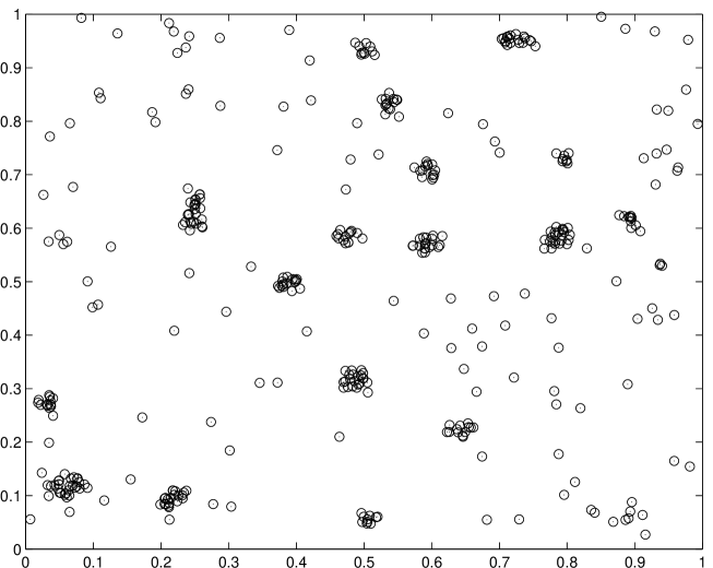
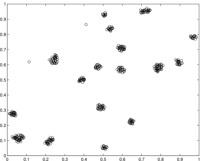
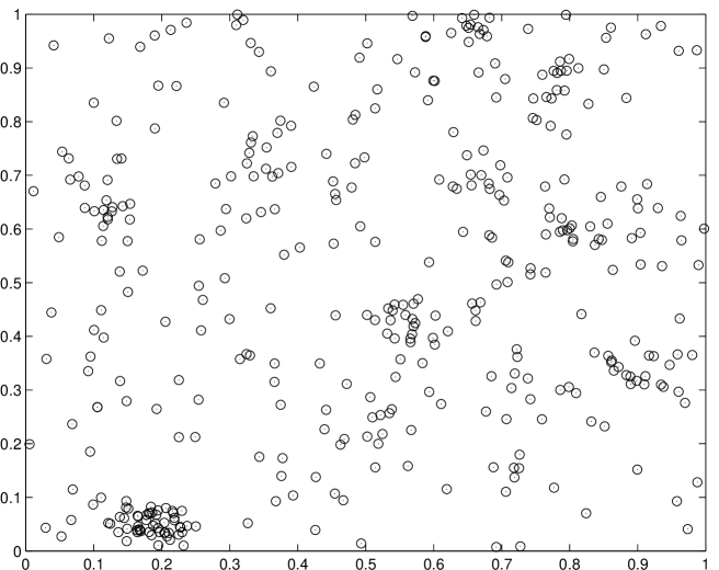
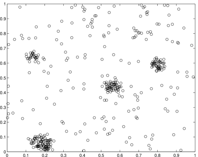
Our paper is structured as follows: In Section 2 we introduce two stochastic individual based models, where every individual is able to sense the average population density in its neighborhood, and respond in terms of increased or decreased stochasticity of its movement. In particular, the diffusivity is reduced in response to higher perceived density. We present a first-order model, where the location of each individual is subject to a density-dependent random walk, and a second-order model, where the density-dependent random walk acts on the velocity variable, together with a density-dependent damping term. The advantage of the second-order model is that it is possible to introduce a cone of vision, which depends on the direction of each individual’s movement. In Section 3 we formally derive the corresponding mean-field limits, leading to a nonlocal, nonlinear diffusion equation for the first-order model, and a nonlinear Fokker-Planck kinetic equation for the second-order model. Moreover, we show that the diffusive limit of the kinetic equation leads to the first-order diffusion equation derived before. Then, in Section 4, we show the existence of weak and measure-valued solutions of the first order mean-field model and perform linear stability analysis of the uniform steady states, finding regimes that correspond to the sought-for pattern formation (direct aggregation). Finally, in Section 5 we present the results of numerical simulations of our models. We performed Langrangian simulations of the first- and second-order agent-based models in a periodic 2D domain, Eulerian simulations of the first-order mean-field model in 1D and 2D periodic domains, and, finally, of the second-order mean-field model in a spatially 1D periodic domain with 1D velocity.

2 The stochastic individual based models

We consider the set of N𝑁N\in\mathbb{N} individuals with time-dependent positions xi(t)dsubscript𝑥𝑖𝑡superscript𝑑x_{i}(t)\in\mathbb{R}^{d}, i=1,,N𝑖1𝑁i=1,\dots,N, with d1𝑑1d\geq 1. Every individual is able to sense the average density of other individuals in its neighborhood, given by

ϑi(t)=1NjiW(xixj),subscriptitalic-ϑ𝑖𝑡1𝑁subscript𝑗𝑖𝑊subscript𝑥𝑖subscript𝑥𝑗\displaystyle\vartheta_{i}(t)=\frac{1}{N}\sum_{j\neq i}W(x_{i}-x_{j})\,, (2.1)

where W(x)=w(|x|)𝑊𝑥𝑤𝑥W(x)=w(|x|) with w:++:𝑤superscriptsuperscriptw:\mathbb{R}^{+}\to\mathbb{R}^{+} is a bounded, nonnegative and nonincreasing weight, integrable on dsuperscript𝑑\mathbb{R}^{d}. A generic example of w𝑤w is the characteristic function of the interval [0,R]0𝑅[0,R], corresponding to the sampling radius R>0𝑅0R>0. The average density ϑisubscriptitalic-ϑ𝑖\vartheta_{i} is then simply the fraction of individuals located within the distance R𝑅R from the i𝑖i-th individual:

ϑi(t)=1N#{j;|xixj|R}.subscriptitalic-ϑ𝑖𝑡1𝑁#𝑗subscript𝑥𝑖subscript𝑥𝑗𝑅\displaystyle\vartheta_{i}(t)=\frac{1}{N}\#\{j;|x_{i}-x_{j}|\leq R\}\,.

For the passage to the mean-field limit N𝑁N\to\infty and the analysis of the resulting equations, we will have to pose certain smoothnes assumptions on W𝑊W, which actually exclude the choice of w𝑤w to be a characteristic function. However, from the modelling point of view this is not a concern.

Let us now introduce our two models:

  • In the first-order model the individual locations are subject to average density-dependent random walk,

    dxi=G(ϑi)dBit,i=1,,N,formulae-sequencedsubscript𝑥𝑖𝐺subscriptitalic-ϑ𝑖dsuperscriptsubscript𝐵𝑖𝑡𝑖1𝑁\displaystyle\,\mathrm{d}x_{i}=G(\vartheta_{i})\,\mathrm{d}B_{i}^{t}\,,\qquad i=1,\dots,N\,, (2.2)

    where Bitsuperscriptsubscript𝐵𝑖𝑡B_{i}^{t} are independent d𝑑d-dimensional Brownian motions and G:++:𝐺superscriptsuperscriptG:\mathbb{R}^{+}\to\mathbb{R}^{+} is a bounded, nonnegative and nonincreasing function. For instance, in the numerical simulations of Section 5 we use G(s)=exp(s/3)𝐺𝑠𝑠3G(s)=\exp(-s/3). However, we as well allow for degeneracy, where G(s)=0𝐺𝑠0G(s)=0 for all ss0>0𝑠subscript𝑠00s\geq s_{0}>0.

  • In the second-order model the individuals are described not only by their locations xi(t)dsubscript𝑥𝑖𝑡superscript𝑑x_{i}(t)\in\mathbb{R}^{d}, but also by the velocities vi(t)dsubscript𝑣𝑖𝑡superscript𝑑v_{i}(t)\in\mathbb{R}^{d}, i=1,,N𝑖1𝑁i=1,\dots,N. The advantage of this description, in contrast to the first-order model, is that every individual has a well defined direction of movement. Therefore, the weight W𝑊W in the calculation of the average densities ϑisubscriptitalic-ϑ𝑖\vartheta_{i} can also depend on the relative angle with respect to the individual’s direction of movement,

    ϑi(t)=1NjiW(xixj,vi),subscriptitalic-ϑ𝑖𝑡1𝑁subscript𝑗𝑖𝑊subscript𝑥𝑖subscript𝑥𝑗subscript𝑣𝑖\displaystyle\vartheta_{i}(t)=\frac{1}{N}\sum_{j\neq i}W(x_{i}-x_{j},v_{i})\,, (2.3)

    with W(x,v)=w(|x|,xv|x||v|)𝑊𝑥𝑣𝑤𝑥𝑥𝑣𝑥𝑣W(x,v)=w\left(|x|,\frac{x\cdot v}{|x||v|}\right). This is important from the modeling point of view, since we can define not only the sampling radius R>0𝑅0R>0, but also a restricted cone of vision with angle α(0,π]𝛼0𝜋\alpha\in(0,\pi]; we set then w(s,z)=χ[0,R](s)χ[cosα,1](z)𝑤𝑠𝑧subscript𝜒0𝑅𝑠subscript𝜒𝛼1𝑧w(s,z)=\chi_{[0,R]}(s)\chi_{[\cos\alpha,1]}(z).

    The velocity in our model is subject to a density-dependent random walk and a density-dependent damping term:

    dxidsubscript𝑥𝑖\displaystyle\,\mathrm{d}x_{i} =\displaystyle= vidt,subscript𝑣𝑖d𝑡\displaystyle v_{i}\,\mathrm{d}t\,, (2.4)
    dvidsubscript𝑣𝑖\displaystyle\,\mathrm{d}v_{i} =\displaystyle= H(ϑi)vidt+G(ϑi)dBit.𝐻subscriptitalic-ϑ𝑖subscript𝑣𝑖d𝑡𝐺subscriptitalic-ϑ𝑖dsuperscriptsubscript𝐵𝑖𝑡\displaystyle-H(\vartheta_{i})v_{i}\,\mathrm{d}t+G(\vartheta_{i})\,\mathrm{d}B_{i}^{t}\,. (2.5)

    The function G𝐺G is as before, while H:++:𝐻superscriptsuperscriptH:\mathbb{R}^{+}\to\mathbb{R}^{+} is a nonnegative and nondecreasing function. The damping term H(ϑi)vi𝐻subscriptitalic-ϑ𝑖subscript𝑣𝑖-H(\vartheta_{i})v_{i} is introduced in order to slow down the agents’ motion when they approach a crowded place. Obviously, this mechanism is not only necessary to allow for formation of aggregates, but also very natural from the modeling point of view.

3 The mean-field limits

3.1 The first-order model

We start with the derivation of the mean-field limit of the first-order model (2.2). Unfortunately, the standard framework of BBGKY hierarchies cannot be applied, since due to the structure of the model it is impossible to obtain a hierarchy where the evolution of the k𝑘k-th marginal is expressed in terms of a finite number of higher-order marginals. Therefore, we have to apply the recently developed technique of introduction of auxiliary variables [3] and their elimination after the mean-field limit passage.

In particular, under the additional assumption WC1(d)𝑊superscript𝐶1superscript𝑑W\in C^{1}(\mathbb{R}^{d}), we extend the model by introducing the average densities ϑisubscriptitalic-ϑ𝑖\vartheta_{i} given by (2.1) as a new set of independent variables, governed by the system of stochastic differential equations

dϑi=1NjiW(xixj)(G(ϑi)dBitG(ϑj)dBjt).dsubscriptitalic-ϑ𝑖1𝑁subscript𝑗𝑖𝑊subscript𝑥𝑖subscript𝑥𝑗𝐺subscriptitalic-ϑ𝑖dsubscriptsuperscript𝐵𝑡𝑖𝐺subscriptitalic-ϑ𝑗dsubscriptsuperscript𝐵𝑡𝑗\displaystyle\,\mathrm{d}\vartheta_{i}=\frac{1}{N}\sum_{j\neq i}\nabla W(x_{i}-x_{j})\left(G(\vartheta_{i})\,\mathrm{d}B^{t}_{i}-G(\vartheta_{j})\,\mathrm{d}B^{t}_{j}\right)\,. (3.1)

Let us point out that the random walks Bitsubscriptsuperscript𝐵𝑡𝑖B^{t}_{i}, Bjtsubscriptsuperscript𝐵𝑡𝑗B^{t}_{j} in (3.1) are correlated with those in (2.2). Using the Itô formula, we turn to the equivalent formulation of the stochastic system (2.2), (3.1) in terms of the corresponding Fokker-Planck equation

fNtsuperscript𝑓𝑁𝑡\displaystyle\frac{\partial f^{N}}{\partial t} =\displaystyle= 12i=1NΔxi(G(ϑi)2fN)+i=1Nϑixi(1NjiW(xixj)G(ϑi)2fN)12superscriptsubscript𝑖1𝑁subscriptΔsubscript𝑥𝑖𝐺superscriptsubscriptitalic-ϑ𝑖2superscript𝑓𝑁superscriptsubscript𝑖1𝑁subscriptitalic-ϑ𝑖subscriptsubscript𝑥𝑖1𝑁subscript𝑗𝑖𝑊subscript𝑥𝑖subscript𝑥𝑗𝐺superscriptsubscriptitalic-ϑ𝑖2superscript𝑓𝑁\displaystyle\frac{1}{2}\sum_{i=1}^{N}\Delta_{x_{i}}\left(G(\vartheta_{i})^{2}f^{N}\right)+\sum_{i=1}^{N}\frac{\partial}{\partial\vartheta_{i}}\nabla_{x_{i}}\cdot\left(\frac{1}{N}\sum_{j\neq i}\nabla W(x_{i}-x_{j})G(\vartheta_{i})^{2}f^{N}\right)
\displaystyle- 1Ni=1Njikiϑjxi(W(xkxi)G(ϑi)2fN)1𝑁superscriptsubscript𝑖1𝑁subscript𝑗𝑖subscript𝑘𝑖subscriptitalic-ϑ𝑗subscriptsubscript𝑥𝑖𝑊subscript𝑥𝑘subscript𝑥𝑖𝐺superscriptsubscriptitalic-ϑ𝑖2superscript𝑓𝑁\displaystyle\frac{1}{N}\sum_{i=1}^{N}\sum_{j\neq i}\sum_{k\neq i}\frac{\partial}{\partial\vartheta_{j}}\nabla_{x_{i}}\cdot\left(\nabla W(x_{k}-x_{i})G(\vartheta_{i})^{2}f^{N}\right)
+\displaystyle+ 12N2i=1Njiki2ϑi2(W(xixk)W(xixl)G(ϑi)2fN)12superscript𝑁2superscriptsubscript𝑖1𝑁subscript𝑗𝑖subscript𝑘𝑖superscript2superscriptsubscriptitalic-ϑ𝑖2𝑊subscript𝑥𝑖subscript𝑥𝑘𝑊subscript𝑥𝑖subscript𝑥𝑙𝐺superscriptsubscriptitalic-ϑ𝑖2superscript𝑓𝑁\displaystyle\frac{1}{2N^{2}}\sum_{i=1}^{N}\sum_{j\neq i}\sum_{k\neq i}\frac{\partial^{2}}{\partial\vartheta_{i}^{2}}\left(\nabla W(x_{i}-x_{k})\cdot\nabla W(x_{i}-x_{l})G(\vartheta_{i})^{2}f^{N}\right)
+\displaystyle+ 12N2i=1Nji2ϑi2(|W(xixj)|2G(ϑj)2fN)12superscript𝑁2superscriptsubscript𝑖1𝑁subscript𝑗𝑖superscript2superscriptsubscriptitalic-ϑ𝑖2superscript𝑊subscript𝑥𝑖subscript𝑥𝑗2𝐺superscriptsubscriptitalic-ϑ𝑗2superscript𝑓𝑁\displaystyle\frac{1}{2N^{2}}\sum_{i=1}^{N}\sum_{j\neq i}\frac{\partial^{2}}{\partial\vartheta_{i}^{2}}\left(|\nabla W(x_{i}-x_{j})|^{2}G(\vartheta_{j})^{2}f^{N}\right)
+\displaystyle+ 12N2i=1Njiki,j2ϑiϑj(W(xixk)W(xjxk)G(ϑk)2fN)12superscript𝑁2superscriptsubscript𝑖1𝑁subscript𝑗𝑖subscript𝑘𝑖𝑗superscript2subscriptitalic-ϑ𝑖subscriptitalic-ϑ𝑗𝑊subscript𝑥𝑖subscript𝑥𝑘𝑊subscript𝑥𝑗subscript𝑥𝑘𝐺superscriptsubscriptitalic-ϑ𝑘2superscript𝑓𝑁\displaystyle\frac{1}{2N^{2}}\sum_{i=1}^{N}\sum_{j\neq i}\sum_{k\neq i,j}\frac{\partial^{2}}{\partial\vartheta_{i}\partial\vartheta_{j}}\left(\nabla W(x_{i}-x_{k})\cdot\nabla W(x_{j}-x_{k})G(\vartheta_{k})^{2}f^{N}\right)
\displaystyle- 1N2i=1Njiki,j2ϑiϑj(W(xixk)W(xixj)G(ϑi)2fN),1superscript𝑁2superscriptsubscript𝑖1𝑁subscript𝑗𝑖subscript𝑘𝑖𝑗superscript2subscriptitalic-ϑ𝑖subscriptitalic-ϑ𝑗𝑊subscript𝑥𝑖subscript𝑥𝑘𝑊subscript𝑥𝑖subscript𝑥𝑗𝐺superscriptsubscriptitalic-ϑ𝑖2superscript𝑓𝑁\displaystyle\frac{1}{N^{2}}\sum_{i=1}^{N}\sum_{j\neq i}\sum_{k\neq i,j}\frac{\partial^{2}}{\partial\vartheta_{i}\partial\vartheta_{j}}\left(\nabla W(x_{i}-x_{k})\cdot\nabla W(x_{i}-x_{j})G(\vartheta_{i})^{2}f^{N}\right)\,,

where fN=fN(t,x1,ϑ1,,xN,ϑN)superscript𝑓𝑁superscript𝑓𝑁𝑡subscript𝑥1subscriptitalic-ϑ1subscript𝑥𝑁subscriptitalic-ϑ𝑁f^{N}=f^{N}(t,x_{1},\vartheta_{1},\dots,x_{N},\vartheta_{N}) is the N𝑁N-particle distribution function. Defining the k𝑘k-particle marginals fkNsubscriptsuperscript𝑓𝑁𝑘f^{N}_{k} by

fkN(t,x1,ϑ1,,xk,ϑk)=d(Nk)(0,)NkfN(t,x1,ϑ1,,xN,ϑN)dϑk+1ϑNdxk+1dxN,subscriptsuperscript𝑓𝑁𝑘𝑡subscript𝑥1subscriptitalic-ϑ1subscript𝑥𝑘subscriptitalic-ϑ𝑘subscriptsuperscript𝑑𝑁𝑘subscriptsuperscript0𝑁𝑘superscript𝑓𝑁𝑡subscript𝑥1subscriptitalic-ϑ1subscript𝑥𝑁subscriptitalic-ϑ𝑁differential-dsubscriptitalic-ϑ𝑘1subscriptitalic-ϑ𝑁differential-dsubscript𝑥𝑘1differential-dsubscript𝑥𝑁\displaystyle f^{N}_{k}(t,x_{1},\vartheta_{1},\dots,x_{k},\vartheta_{k})=\int_{\mathbb{R}^{d(N-k)}}\int_{(0,\infty)^{N-k}}f^{N}(t,x_{1},\vartheta_{1},\dots,x_{N},\vartheta_{N})\,\mathrm{d}\vartheta_{k+1}\dots\vartheta_{N}\,\mathrm{d}x_{k+1}\dots\,\mathrm{d}x_{N}\,,

we obtain the so-called BBGKY-hierarchy for the system (fkN)k=1Nsuperscriptsubscriptsubscriptsuperscript𝑓𝑁𝑘𝑘1𝑁(f^{N}_{k})_{k=1}^{N}. In particular, the equation for f1=f1(t,x,ϑ)subscript𝑓1subscript𝑓1𝑡𝑥italic-ϑf_{1}=f_{1}(t,x,\vartheta) reads

f1Ntsubscriptsuperscript𝑓𝑁1𝑡\displaystyle\frac{\partial f^{N}_{1}}{\partial t} =\displaystyle= 12Δx(G(ϑ)2f1N)+ϑx(G(ϑ)2d0W(xy)f2N(x,ϑ,y,σ)dσdy)12subscriptΔ𝑥𝐺superscriptitalic-ϑ2subscriptsuperscript𝑓𝑁1italic-ϑsubscript𝑥𝐺superscriptitalic-ϑ2subscriptsuperscript𝑑superscriptsubscript0𝑊𝑥𝑦subscriptsuperscript𝑓𝑁2𝑥italic-ϑ𝑦𝜎differential-d𝜎differential-d𝑦\displaystyle\frac{1}{2}\Delta_{x}\left(G(\vartheta)^{2}f^{N}_{1}\right)+\frac{\partial}{\partial\vartheta}\nabla_{x}\cdot\left(G(\vartheta)^{2}\int_{\mathbb{R}^{d}}\int_{0}^{\infty}\nabla W(x-y)f^{N}_{2}(x,\vartheta,y,\sigma)\,\mathrm{d}\sigma\,\mathrm{d}y\right) (3.2)
+\displaystyle+ 122ϑ2(G(ϑ)2dd00W(xy)W(xz)f3N(x,ϑ,y,σ,z,τ)dσdτdydz)12superscript2superscriptitalic-ϑ2𝐺superscriptitalic-ϑ2subscriptsuperscript𝑑subscriptsuperscript𝑑superscriptsubscript0superscriptsubscript0𝑊𝑥𝑦𝑊𝑥𝑧subscriptsuperscript𝑓𝑁3𝑥italic-ϑ𝑦𝜎𝑧𝜏differential-d𝜎differential-d𝜏differential-d𝑦differential-d𝑧\displaystyle\frac{1}{2}\frac{\partial^{2}}{\partial\vartheta^{2}}\left(G(\vartheta)^{2}\int_{\mathbb{R}^{d}}\int_{\mathbb{R}^{d}}\int_{0}^{\infty}\int_{0}^{\infty}\nabla W(x-y)\nabla W(x-z)f^{N}_{3}(x,\vartheta,y,\sigma,z,\tau)\,\mathrm{d}\sigma\,\mathrm{d}\tau\,\mathrm{d}y\,\mathrm{d}z\right)
+\displaystyle+ 12N2ϑ2(d0G(ϑ)2|W(xy)|2f2N(x,ϑ,y,σ)dσdy),12𝑁superscript2superscriptitalic-ϑ2subscriptsuperscript𝑑superscriptsubscript0𝐺superscriptitalic-ϑ2superscript𝑊𝑥𝑦2subscriptsuperscript𝑓𝑁2𝑥italic-ϑ𝑦𝜎differential-d𝜎differential-d𝑦\displaystyle\frac{1}{2N}\frac{\partial^{2}}{\partial\vartheta^{2}}\left(\int_{\mathbb{R}^{d}}\int_{0}^{\infty}G(\vartheta)^{2}|\nabla W(x-y)|^{2}f^{N}_{2}(x,\vartheta,y,\sigma)\,\mathrm{d}\sigma\,\mathrm{d}y\right)\,,

where we, for the sake of legibility, dropped the indices at x1subscript𝑥1x_{1} and ϑ1subscriptitalic-ϑ1\vartheta_{1}. Now, we pass formally to the limit N𝑁N\to\infty, assuming that limNfkN=fksubscript𝑁subscriptsuperscript𝑓𝑁𝑘subscript𝑓𝑘\lim_{N\to\infty}f^{N}_{k}=f_{k} for all k1𝑘1k\geq 1. Moreover, we admit the usual molecular chaos assumption about vanishing particle correlations as N𝑁N\to\infty,

fk(t,x1,ϑ1,,xk,ϑk)=i=1kf1(t,xi,ϑi)for all k2.formulae-sequencesubscript𝑓𝑘𝑡subscript𝑥1subscriptitalic-ϑ1subscript𝑥𝑘subscriptitalic-ϑ𝑘superscriptsubscriptproduct𝑖1𝑘subscript𝑓1𝑡subscript𝑥𝑖subscriptitalic-ϑ𝑖for all 𝑘2\displaystyle f_{k}(t,x_{1},\vartheta_{1},\dots,x_{k},\vartheta_{k})=\prod_{i=1}^{k}f_{1}(t,x_{i},\vartheta_{i})\qquad\mbox{for all }k\geq 2\,.

Then, one obtains from (3.2) the one-particle equation

f1t=12Δx(G(ϑ)2f1)+ϑ(G(ϑ)2(Wf1)f1)+122ϑ2(G(ϑ)2|Wf1|2f1),subscript𝑓1𝑡12subscriptΔ𝑥𝐺superscriptitalic-ϑ2subscript𝑓1italic-ϑ𝐺superscriptitalic-ϑ2𝑊subscript𝑓1subscript𝑓112superscript2superscriptitalic-ϑ2𝐺superscriptitalic-ϑ2superscript𝑊subscript𝑓12subscript𝑓1\displaystyle\frac{\partial f_{1}}{\partial t}=\frac{1}{2}\Delta_{x}\left(G(\vartheta)^{2}f_{1}\right)+\frac{\partial}{\partial\vartheta}\nabla\cdot\left(G(\vartheta)^{2}(\nabla W\circledast f_{1})f_{1}\right)+\frac{1}{2}\frac{\partial^{2}}{\partial\vartheta^{2}}\left(G(\vartheta)^{2}|\nabla W\circledast f_{1}|^{2}f_{1}\right)\,, (3.3)

where the operator \circledast is defined as

Wf1(t,x)=d0W(xy)f1(t,y,ϑ)dϑdy.𝑊subscript𝑓1𝑡𝑥subscriptsuperscript𝑑superscriptsubscript0𝑊𝑥𝑦subscript𝑓1𝑡𝑦italic-ϑdifferential-ditalic-ϑdifferential-d𝑦\displaystyle\nabla W\circledast f_{1}(t,x)=\int_{\mathbb{R}^{d}}\int_{0}^{\infty}\nabla W(x-y)f_{1}(t,y,\vartheta)\,\mathrm{d}\vartheta\,\mathrm{d}y\,.

Finally, we reduce (3.3) to obtain the standard mean-field description of the system (2.2) by removing the auxiliary variable ϑitalic-ϑ\vartheta. Indeed, a relatively lengthy, but straight-forward formal calculation shows that (3.3) posesses weak solutions of the form

f1(t,x,ϑ)=ϱ(t,x)δ(ϑWϱ(t,x)),with Wϱ(t,x)=dW(xy)ϱ(t,y)dyformulae-sequencesubscript𝑓1𝑡𝑥italic-ϑitalic-ϱ𝑡𝑥𝛿italic-ϑ𝑊italic-ϱ𝑡𝑥with 𝑊italic-ϱ𝑡𝑥subscriptsuperscript𝑑𝑊𝑥𝑦italic-ϱ𝑡𝑦differential-d𝑦\displaystyle f_{1}(t,x,\vartheta)=\varrho(t,x)\delta(\vartheta-W\ast\varrho(t,x))\,,\qquad\mbox{with }W\ast\varrho(t,x)=\int_{\mathbb{R}^{d}}W(x-y)\varrho(t,y)\,\mathrm{d}y

and ϱ=ϱ(t,x)italic-ϱitalic-ϱ𝑡𝑥\varrho=\varrho(t,x) satisfies the nonlinear diffusion equation

ϱt=12Δx(G(Wϱ)2ϱ).italic-ϱ𝑡12subscriptΔ𝑥𝐺superscript𝑊italic-ϱ2italic-ϱ\displaystyle\frac{\partial\varrho}{\partial t}=\frac{1}{2}\Delta_{x}\left(G(W\ast\varrho)^{2}\varrho\right)\,. (3.4)

3.2 The second-order model

With the same procedure as before we derive the formal mean-field limit of the model (2.4)–(2.5). We omit the details here and immediately give the resulting kinetic Fokker-Planck equation for the particle distribution function f=f(t,x,v)𝑓𝑓𝑡𝑥𝑣f=f(t,x,v),

ft+vxf=v(H(Wf)vf+12v(G(Wf)2f)),𝑓𝑡𝑣subscript𝑥𝑓subscript𝑣𝐻𝑊𝑓𝑣𝑓12subscript𝑣𝐺superscript𝑊𝑓2𝑓\displaystyle\frac{\partial f}{\partial t}+v\cdot\nabla_{x}f=\nabla_{v}\cdot\left(H(W\circledast f)vf+\frac{1}{2}\nabla_{v}\left(G(W\circledast f)^{2}f\right)\right)\,, (3.5)

where, with a slight abuse of notation, the convolution operator \circledast is defined as

Wf(t,x,v)=ddW(xy,v)f(t,y,w)dwdy.𝑊𝑓𝑡𝑥𝑣subscriptsuperscript𝑑subscriptsuperscript𝑑𝑊𝑥𝑦𝑣𝑓𝑡𝑦𝑤differential-d𝑤differential-d𝑦\displaystyle W\circledast f(t,x,v)=\int_{\mathbb{R}^{d}}\int_{\mathbb{R}^{d}}W(x-y,v)f(t,y,w)\,\mathrm{d}w\,\mathrm{d}y\,.

Let us make the following observation: If the weight W𝑊W does not depend on v𝑣v, such that Wf𝑊𝑓W\circledast f does not depend on v𝑣v as well and Wf(t,x)=Wϱ(t,x)𝑊𝑓𝑡𝑥𝑊italic-ϱ𝑡𝑥W\circledast f(t,x)=W\ast\varrho(t,x), we can write the (non-closed) system for the mass, momentum and energy densities

ϱ(t,x)=df(t,x,v)dv,ϱu(t,x)=df(t,x,v)vdv,ϱE(t,x)=12df(t,x,v)|v|2dv,formulae-sequenceitalic-ϱ𝑡𝑥subscriptsuperscript𝑑𝑓𝑡𝑥𝑣differential-d𝑣formulae-sequenceitalic-ϱ𝑢𝑡𝑥subscriptsuperscript𝑑𝑓𝑡𝑥𝑣𝑣differential-d𝑣italic-ϱ𝐸𝑡𝑥12subscriptsuperscript𝑑𝑓𝑡𝑥𝑣superscript𝑣2differential-d𝑣\displaystyle\varrho(t,x)=\int_{\mathbb{R}^{d}}f(t,x,v)\,\mathrm{d}v\,,\qquad\varrho u(t,x)=\int_{\mathbb{R}^{d}}f(t,x,v)v\,\mathrm{d}v\,,\qquad\varrho E(t,x)=\frac{1}{2}\int_{\mathbb{R}^{d}}f(t,x,v)|v|^{2}\,\mathrm{d}v\,, (3.6)

associated with the solution f𝑓f of (3.5) as

ϱt+x(ϱu)italic-ϱ𝑡subscript𝑥italic-ϱ𝑢\displaystyle\frac{\partial\varrho}{\partial t}+\nabla_{x}\cdot(\varrho u) =\displaystyle= 0,0\displaystyle 0\,, (3.7)
(ϱu)t+x(df(t,x,v)vvdv)italic-ϱ𝑢𝑡subscript𝑥subscriptsuperscript𝑑tensor-product𝑓𝑡𝑥𝑣𝑣𝑣differential-d𝑣\displaystyle\frac{\partial(\varrho u)}{\partial t}+\nabla_{x}\cdot\left(\int_{\mathbb{R}^{d}}f(t,x,v)v\otimes v\,\mathrm{d}v\right) =\displaystyle= H(Wϱ)ϱu,𝐻𝑊italic-ϱitalic-ϱ𝑢\displaystyle-H(W\ast\varrho)\varrho u\,, (3.8)
(ϱE)t+x(12df(t,x,v)|v|2vdv)italic-ϱ𝐸𝑡subscript𝑥12subscriptsuperscript𝑑𝑓𝑡𝑥𝑣superscript𝑣2𝑣differential-d𝑣\displaystyle\frac{\partial(\varrho E)}{\partial t}+\nabla_{x}\cdot\left(\frac{1}{2}\int_{\mathbb{R}^{d}}f(t,x,v)|v|^{2}v\,\mathrm{d}v\right) =\displaystyle= 2H(Wϱ)ϱE+d2G(Wϱ)2ϱ.2𝐻𝑊italic-ϱitalic-ϱ𝐸𝑑2𝐺superscript𝑊italic-ϱ2italic-ϱ\displaystyle-2H(W\ast\varrho)\varrho E+\frac{d}{2}G(W\ast\varrho)^{2}\varrho\,. (3.9)

We observe that only mass is conserved, while momentum and energy are not (neither locally nor globally). Indeed, the momentum is dissipated due to the “friction” term, whose strength depends non-locally on ϱitalic-ϱ\varrho due to H(Wϱ)𝐻𝑊italic-ϱH(W\ast\varrho). The energy is, on one hand, dissipated due to the same term, on the other hand is created due to the diffusive term in (3.5), at the rate d2EG(Wϱ)2𝑑2𝐸𝐺superscript𝑊italic-ϱ2\frac{d}{2E}G(W\ast\varrho)^{2}. In equilibrium, we have H(Wϱ)ϱu=0𝐻𝑊italic-ϱitalic-ϱ𝑢0H(W\ast\varrho)\varrho u=0, which means that we either have empty regions (ϱ=0italic-ϱ0\varrho=0) or regions with positive density, but zero velocity. In these populated regions the equilibrium energy is given by

E=E[ϱ]=d4G(Wϱ)2H(Wϱ).𝐸𝐸delimited-[]italic-ϱ𝑑4𝐺superscript𝑊italic-ϱ2𝐻𝑊italic-ϱ\displaystyle E=E[\varrho]=\frac{d}{4}\frac{G(W\ast\varrho)^{2}}{H(W\ast\varrho)}\,.

3.3 Diffusive limit of the second-order model (3.5)

We show that the first-order model (3.4) is obtained from (3.5) in the formal diffusive limit, under the assumption that the weight W𝑊W does not depend on v𝑣v, which we make for all of this section. Let us recall that then Wf𝑊𝑓W\circledast f does not depend on v𝑣v as well and Wf(t,x)=Wϱ(t,x)𝑊𝑓𝑡𝑥𝑊italic-ϱ𝑡𝑥W\circledast f(t,x)=W\ast\varrho(t,x), with ϱitalic-ϱ\varrho defined by (3.6).

We start by observing that the equilibria of the collision operator of (3.5) are given by the local Maxwellians

[ϱ](v)=(H(Wϱ)2πG(Wϱ)2)d/2ϱexp(H(Wϱ)G(Wϱ)2|v|2).delimited-[]italic-ϱ𝑣superscript𝐻𝑊italic-ϱ2𝜋𝐺superscript𝑊italic-ϱ2𝑑2italic-ϱ𝐻𝑊italic-ϱ𝐺superscript𝑊italic-ϱ2superscript𝑣2\displaystyle\mathcal{M}[\varrho](v)=\left(\frac{H(W\ast\varrho)}{2\pi G(W\ast\varrho)^{2}}\right)^{d/2}\varrho\exp\left(-\frac{H(W\ast\varrho)}{G(W\ast\varrho)^{2}}|v|^{2}\right)\,. (3.10)

Therefore, at equilibrium the mean velocity u𝑢u vanishes if ϱ0italic-ϱ0\varrho\neq 0, and the “statistical temperature” T𝑇T, defined by

d2ϱT=12d[ϱ](v)|v|2dv,𝑑2italic-ϱ𝑇12subscriptsuperscript𝑑delimited-[]italic-ϱ𝑣superscript𝑣2differential-d𝑣\displaystyle\frac{d}{2}\varrho T=\frac{1}{2}\int_{\mathbb{R}^{d}}\mathcal{M}[\varrho](v)|v|^{2}\,\mathrm{d}v\,,

depends non-locally on ϱitalic-ϱ\varrho and is given by

T=T[Wϱ]=G(Wϱ)22H(Wϱ).𝑇𝑇delimited-[]𝑊italic-ϱ𝐺superscript𝑊italic-ϱ22𝐻𝑊italic-ϱ\displaystyle T=T[W\ast\varrho]=\frac{G(W\ast\varrho)^{2}}{2H(W\ast\varrho)}\,. (3.11)

Consequently, in crowded regions (where Wϱ𝑊italic-ϱW\ast\varrho is high) the temperature is low (“freezing of the aggregates”), while the unhabitated regions are “hot”.

We introduce the diffusive scaling with the small parameter ε>0𝜀0\varepsilon>0 to (3.5),

ε2ft+εvxf=v(H(Wϱ)vf+12v(G(Wϱ)2f)),superscript𝜀2𝑓𝑡𝜀𝑣subscript𝑥𝑓subscript𝑣𝐻𝑊italic-ϱ𝑣𝑓12subscript𝑣𝐺superscript𝑊italic-ϱ2𝑓\displaystyle\varepsilon^{2}\frac{\partial f}{\partial t}+\varepsilon v\cdot\nabla_{x}f=\nabla_{v}\cdot\left(H(W\ast\varrho)vf+\frac{1}{2}\nabla_{v}\left(G(W\ast\varrho)^{2}f\right)\right)\,,

and consider the Hilbert expansion in terms of ε𝜀\varepsilon, f=[ϱ]+εg𝑓delimited-[]italic-ϱ𝜀𝑔f=\mathcal{M}[\varrho]+\varepsilon g, where [ϱ]delimited-[]italic-ϱ\mathcal{M}[\varrho] is given by (3.10). Moreover, we perform the Taylor expansion of H(Wϱ)𝐻𝑊italic-ϱH(W\ast\varrho), which we formally write as

H(Wϱ)=H0+εH1+𝒪(ε2),𝐻𝑊italic-ϱsubscript𝐻0𝜀subscript𝐻1𝒪superscript𝜀2\displaystyle H(W\ast\varrho)=H_{0}+\varepsilon H_{1}+\mathcal{O}(\varepsilon^{2})\,,

with

H0=H(Wϱ),H1=H(Wϱ)Wϱg,formulae-sequencesubscript𝐻0𝐻𝑊subscriptitalic-ϱsubscript𝐻1superscript𝐻𝑊subscriptitalic-ϱ𝑊subscriptitalic-ϱ𝑔\displaystyle H_{0}=H(W\ast\varrho_{\mathcal{M}})\,,\qquad H_{1}=H^{\prime}(W\ast\varrho_{\mathcal{M}})W\ast\varrho_{g}\,,

and similarly for G(Wϱ)=G0+εG1+𝒪(ε2)𝐺𝑊italic-ϱsubscript𝐺0𝜀subscript𝐺1𝒪superscript𝜀2G(W\ast\varrho)=G_{0}+\varepsilon G_{1}+\mathcal{O}(\varepsilon^{2}). Here, ϱsubscriptitalic-ϱ\varrho_{\mathcal{M}} and ϱgsubscriptitalic-ϱ𝑔\varrho_{g} denote the velocity averages of the lowest order terms in the expansion, i.e.

ϱ=d[ϱ]dv,ϱg=dgdv.formulae-sequencesubscriptitalic-ϱsubscriptsuperscript𝑑delimited-[]italic-ϱdifferential-d𝑣subscriptitalic-ϱ𝑔subscriptsuperscript𝑑𝑔differential-d𝑣\displaystyle\varrho_{\mathcal{M}}=\int_{\mathbb{R}^{d}}\mathcal{M}[\varrho]\,\mathrm{d}v,\quad\varrho_{g}=\int_{\mathbb{R}^{d}}g\,\mathrm{d}v.

Then, collecting terms of order ε𝜀\varepsilon, we obtain

vx=v(H0vg+H1v+12v(G0g+G1)),𝑣subscript𝑥subscript𝑣subscript𝐻0𝑣𝑔subscript𝐻1𝑣12subscript𝑣subscript𝐺0𝑔subscript𝐺1\displaystyle v\cdot\nabla_{x}\mathcal{M}=\nabla_{v}\cdot\left(H_{0}vg+H_{1}v\mathcal{M}+\frac{1}{2}\nabla_{v}\left(G_{0}g+G_{1}\mathcal{M}\right)\right)\,,

which yields, after multiplication by v𝑣v and integration,

d2x(ϱT[Wϱ])=xdvvdv=H0dgvdv,𝑑2subscript𝑥subscriptitalic-ϱ𝑇delimited-[]𝑊subscriptitalic-ϱsubscript𝑥subscriptsuperscript𝑑tensor-product𝑣𝑣differential-d𝑣subscript𝐻0subscriptsuperscript𝑑𝑔𝑣differential-d𝑣\displaystyle\frac{d}{2}\nabla_{x}\left(\varrho_{\mathcal{M}}T[W\ast\varrho_{\mathcal{M}}]\right)=\nabla_{x}\cdot\int_{\mathbb{R}^{d}}\mathcal{M}v\otimes v\,\mathrm{d}v=-H_{0}\int_{\mathbb{R}^{d}}gv\,\mathrm{d}v\,, (3.12)

with T[Wϱ]𝑇delimited-[]𝑊subscriptitalic-ϱT[W\ast\varrho_{\mathcal{M}}] given by (3.11). Collecting terms of order ε2superscript𝜀2\varepsilon^{2} and integrating with respect to v𝑣v, we obtain

ϱt+xdgvdv=0,subscriptitalic-ϱ𝑡subscript𝑥subscriptsuperscript𝑑𝑔𝑣differential-d𝑣0\displaystyle\frac{\partial\varrho_{\mathcal{M}}}{\partial t}+\nabla_{x}\cdot\int_{\mathbb{R}^{d}}gv\,\mathrm{d}v=0\,,

and using (3.12), we finally obtain the nonlinear diffusion equation

ϱtd2x(1H(Wϱ)x(T[Wϱ]ϱ))=0.subscriptitalic-ϱ𝑡𝑑2subscript𝑥1𝐻𝑊subscriptitalic-ϱsubscript𝑥𝑇delimited-[]𝑊subscriptitalic-ϱsubscriptitalic-ϱ0\displaystyle\frac{\partial\varrho_{\mathcal{M}}}{\partial t}-\frac{d}{2}\nabla_{x}\cdot\left(\frac{1}{H(W\ast\varrho_{\mathcal{M}})}\nabla_{x}\left(T[W\ast\varrho_{\mathcal{M}}]\varrho_{\mathcal{M}}\right)\right)=0\,. (3.13)

Observe that with the choice Hconst.𝐻const.H\equiv\mbox{const.}, (3.13) reduces to (3.4), possibly up to a linear rescaling of time.

4 Mathematical analysis of the first-order model

In this section we show the existence of weak solutions of the first-order nonlinear diffusion equation (3.4) and some asymptotic properties of these solutions. For simplicity, we consider the full space setting Ω=dΩsuperscript𝑑\Omega=\mathbb{R}^{d}, d1𝑑1d\geq 1, but our analysis can be easily adapted to the case of a bounded domain ΩΩ\Omega with homogeneous Neumann boundary conditions, or to the case of periodic boundary conditions, as in the numerical examples of Section 5.

To simplify the notation, we set F(z):=12G(z)2assign𝐹𝑧12𝐺superscript𝑧2F(z):=\frac{1}{2}G(z)^{2}, thus we rewrite (3.4) as

ϱt=Δ(F(Wϱ)ϱ),italic-ϱ𝑡Δ𝐹𝑊italic-ϱitalic-ϱ\displaystyle\frac{\partial\varrho}{\partial t}=\Delta\left(F(W\ast\varrho)\varrho\right)\,, (4.1)

subject to the initial condition

ϱ(t=0)=ϱ0.italic-ϱ𝑡0subscriptitalic-ϱ0\displaystyle\varrho(t=0)=\varrho_{0}\,. (4.2)

For the rest of this Section, and without further notice, we make the following reasonable assumptions on F𝐹F and W𝑊W:

  • F:++:𝐹superscriptsuperscriptF:\mathbb{R}^{+}\rightarrow\mathbb{R}^{+} is a bounded, nonnegative and nonincreasing function. Let us note that we allow for degeneracy in (3.4), i.e., there might exist an s0>0subscript𝑠00s_{0}>0 such that F(s)=0𝐹𝑠0F(s)=0 for all s>s0𝑠subscript𝑠0s>s_{0}.

  • F𝐹F is continuously differentiable with globally Lipschitz continuous derivative and G=2F𝐺2𝐹G=\sqrt{2F} is globally Lipschitz continuous.

  • WW1,(d)H2(d)𝑊superscript𝑊1superscript𝑑superscript𝐻2superscript𝑑W\in W^{1,\infty}(\mathbb{R}^{d})\cap H^{2}(\mathbb{R}^{d}).

Definition 1

We call ϱL(0,T;𝒫(Ω))italic-ϱsuperscript𝐿0𝑇𝒫Ω\varrho\in L^{\infty}(0,T;\mathcal{P}(\Omega)), where 𝒫(Ω)𝒫Ω\mathcal{P}(\Omega) denotes the set of probability measures on ΩΩ\Omega, a weak solution of (4.1) subject to the initial condition (4.2) with 0ϱ0L2(Ω)𝒫(Ω)0subscriptitalic-ϱ0superscript𝐿2Ω𝒫Ω0\leq\varrho_{0}\in L^{2}(\Omega)\cap\mathcal{P}(\Omega), if (F(Wϱ)ϱ)L2(0,T;L2(Ω))𝐹𝑊italic-ϱitalic-ϱsuperscript𝐿20𝑇superscript𝐿2Ω\nabla(F(W\ast\varrho)\varrho)\in L^{2}(0,T;L^{2}(\Omega)) and for every smooth, compactly supported test function φCc([0,T)×Ω)𝜑subscriptsuperscript𝐶𝑐0𝑇Ω\varphi\in C^{\infty}_{c}([0,T)\times\Omega) we have

0Ωϱφtdxdt+Ωϱ0φ(t=0)dx=0Ω(F(Wϱ)ϱ)φdxdt.superscriptsubscript0subscriptΩitalic-ϱ𝜑𝑡differential-d𝑥differential-d𝑡subscriptΩsubscriptitalic-ϱ0𝜑𝑡0differential-d𝑥superscriptsubscript0subscriptΩ𝐹𝑊italic-ϱitalic-ϱ𝜑d𝑥d𝑡\displaystyle\int_{0}^{\infty}\int_{\Omega}\varrho\frac{\partial\varphi}{\partial t}\,\mathrm{d}x\,\mathrm{d}t+\int_{\Omega}\varrho_{0}\varphi(t=0)\,\mathrm{d}x=\int_{0}^{\infty}\int_{\Omega}\nabla(F(W\ast\varrho)\varrho)\cdot\nabla\varphi\,\mathrm{d}x\,\mathrm{d}t\,. (4.3)

The proof of existence of weak solutions in the sense of Definition 1 will be performed in two steps. First, we consider an approximating, uniformly parabolic equation, and prove the existence of its solutions. Then, we remove the approximation in a limiting procedure, to obtain global in time distributional solutions.

4.1 Approximation

In order to obtain a uniformly positive diffusion coefficient, we use the approximation Fε(z):=F(z)+εassignsubscript𝐹𝜀𝑧𝐹𝑧𝜀F_{\varepsilon}(z):=F(z)+\varepsilon for ε>0𝜀0\varepsilon>0, and analyze the approximating equation ϱt=Δ(Fε(Wϱ)ϱ)italic-ϱ𝑡Δsubscript𝐹𝜀𝑊italic-ϱitalic-ϱ\frac{\partial\varrho}{\partial t}=\Delta\left(F_{\varepsilon}(W\ast\varrho)\varrho\right), which we write in the Fokker-Planck form

ϱt=(ϱFε(Wϱ)+Fε(Wϱ)ϱ)italic-ϱ𝑡italic-ϱsubscript𝐹𝜀𝑊italic-ϱsubscript𝐹𝜀𝑊italic-ϱitalic-ϱ\displaystyle\frac{\partial\varrho}{\partial t}=\nabla\cdot\bigl{(}\varrho\nabla F_{\varepsilon}(W\ast\varrho)+F_{\varepsilon}(W\ast\varrho)\nabla\varrho\bigr{)} (4.4)

subject to the inital condition

ϱ(t=0)=ϱ0.italic-ϱ𝑡0subscriptitalic-ϱ0\displaystyle\varrho(t=0)=\varrho_{0}\,. (4.5)
Theorem 1

For every ε>0𝜀0\varepsilon>0, T>0𝑇0T>0 and ϱ0L2(Ω)𝒫(Ω)subscriptitalic-ϱ0superscript𝐿2Ω𝒫Ω\varrho_{0}\in L^{2}(\Omega)\cap{\cal P}(\Omega) there exists a nonnegative weak solution

ϱεL2(0,T;H1(Ω))H1(0,T;H1(Ω))L(0,T;𝒫(Ω))superscriptitalic-ϱ𝜀superscript𝐿20𝑇superscript𝐻1Ωsuperscript𝐻10𝑇superscript𝐻1Ωsuperscript𝐿0𝑇𝒫Ω\displaystyle\varrho^{\varepsilon}\in L^{2}(0,T;H^{1}(\Omega))\cap H^{1}(0,T;H^{-1}(\Omega))\cap L^{\infty}(0,T;{\cal P}(\Omega))

of (4.4) in the sense of Definition 1 (with Fεsubscript𝐹𝜀F_{\varepsilon} in place of F𝐹F).

Proof: The solution is constructed as a fixed point of the map Θ:uϱ:Θmaps-to𝑢italic-ϱ\Theta:u\mapsto\varrho, defined on the convex, bounded set

R:={uL2((0,T)×Ω);uL(0,T;L2(Ω))R and u(t,)𝒫(Ω) for a.e. t(0,T)}assignsubscript𝑅formulae-sequence𝑢superscript𝐿20𝑇Ωsubscriptnorm𝑢superscript𝐿0𝑇superscript𝐿2Ω𝑅 and 𝑢𝑡𝒫Ω for a.e. 𝑡0𝑇{\cal B}_{R}:=\{u\in L^{2}((0,T)\times\Omega)\,;~{}\left\|u\right\|_{L^{\infty}(0,T;L^{2}(\Omega))}\leq R\mbox{ and }u(t,\cdot)\in\mathcal{P}(\Omega)\text{ for a.e. }t\in(0,T)\}

with R>0𝑅0R>0 to be specified later, where ϱ=Θ(u)italic-ϱΘ𝑢\varrho=\Theta(u) is the unique solution of the Fokker-Planck equation

ϱt=(ϱFε(Wu)+Fε(Wu)ϱ).italic-ϱ𝑡italic-ϱsubscript𝐹𝜀𝑊𝑢subscript𝐹𝜀𝑊𝑢italic-ϱ\displaystyle\frac{\partial\varrho}{\partial t}=\nabla\cdot\bigl{(}\varrho\nabla F_{\varepsilon}(W\ast u)+F_{\varepsilon}(W\ast u)\nabla\varrho\bigr{)}\,. (4.6)

Due to the assumed properties of W𝑊W and F𝐹F, the diffusion coefficient satisfies Fε(Wu)L((0,T)×Ω)subscript𝐹𝜀𝑊𝑢superscript𝐿0𝑇ΩF_{\varepsilon}(W\ast u)\in L^{\infty}((0,T)\times\Omega) and is bounded below by ε𝜀\varepsilon, and the convection coefficient Fε(Wu)L((0,T)×Ω)subscript𝐹𝜀𝑊𝑢superscript𝐿0𝑇Ω\nabla F_{\varepsilon}(W\ast u)\in L^{\infty}((0,T)\times\Omega). Thus, (4.6) is a linear, uniformly parabolic equation with bounded coefficients, and the standard theory [5] implies the existence and uniqueness of the global, nonnegative weak solution

ϱL(0,T;L2(Ω))L2(0,T;H1(Ω))H1(0,T;H1(Ω)),italic-ϱsuperscript𝐿0𝑇superscript𝐿2Ωsuperscript𝐿20𝑇superscript𝐻1Ωsuperscript𝐻10𝑇superscript𝐻1Ω\displaystyle\varrho\in L^{\infty}(0,T;L^{2}(\Omega))\cap L^{2}(0,T;H^{1}(\Omega))\cap H^{1}(0,T;H^{-1}(\Omega)), (4.7)

such that ϱ(,t)𝒫(Ω)italic-ϱ𝑡𝒫Ω\varrho(\cdot,t)\in{\cal P}(\Omega) for almost every t0𝑡0t\geq 0. Therefore, ΘΘ\Theta is well defined on Rsubscript𝑅{\cal B}_{R} and, as can be easily proven, is continuous there.

In order to apply the Schauder fixed point theorem (cf. [4]), we need to show that ΘΘ\Theta maps Rsubscript𝑅{\cal B}_{R} into a compact subset of itself. The key point is the following a-priori estimate, obtained by using ϱitalic-ϱ\varrho as a test function for (4.6) (note that due to (4.7), ϱitalic-ϱ\varrho is indeed an admissible test function):

0sΩϱϱtdxdt+Ωϱ02dx+0sΩFε|ϱ|2dxdt=0sΩϱFεϱdxdt,superscriptsubscript0𝑠subscriptΩitalic-ϱitalic-ϱ𝑡differential-d𝑥differential-d𝑡subscriptΩsuperscriptsubscriptitalic-ϱ02differential-d𝑥superscriptsubscript0𝑠subscriptΩsubscript𝐹𝜀superscriptitalic-ϱ2differential-d𝑥differential-d𝑡superscriptsubscript0𝑠subscriptΩitalic-ϱsubscript𝐹𝜀italic-ϱd𝑥d𝑡\displaystyle\int_{0}^{s}\int_{\Omega}\varrho\frac{\partial\varrho}{\partial t}\,\mathrm{d}x\,\mathrm{d}t+\int_{\Omega}\varrho_{0}^{2}\,\mathrm{d}x+\int_{0}^{s}\int_{\Omega}F_{\varepsilon}|\nabla\varrho|^{2}\,\mathrm{d}x\,\mathrm{d}t=-\int_{0}^{s}\int_{\Omega}\varrho\nabla F_{\varepsilon}\cdot\nabla\varrho\,\mathrm{d}x\,\mathrm{d}t\,,

for s(0,T)𝑠0𝑇s\in(0,T), where we introduced the shorthand notation Fε:=Fε(Wu)assignsubscript𝐹𝜀subscript𝐹𝜀𝑊𝑢F_{\varepsilon}:=F_{\varepsilon}(W\ast u). Now we use the identity

0sΩϱϱtdxdt=120sddt(Ωϱ2dx)dt=12Ωϱ(x,s)2dx12Ωϱ02dxsuperscriptsubscript0𝑠subscriptΩitalic-ϱitalic-ϱ𝑡differential-d𝑥differential-d𝑡12superscriptsubscript0𝑠𝑑𝑑𝑡subscriptΩsuperscriptitalic-ϱ2differential-d𝑥differential-d𝑡12subscriptΩitalic-ϱsuperscript𝑥𝑠2differential-d𝑥12subscriptΩsuperscriptsubscriptitalic-ϱ02differential-d𝑥\displaystyle\int_{0}^{s}\int_{\Omega}\varrho\frac{\partial\varrho}{\partial t}\,\mathrm{d}x\,\mathrm{d}t=\frac{1}{2}\int_{0}^{s}\frac{d}{dt}\left(\int_{\Omega}\varrho^{2}\,\mathrm{d}x\right)\,\mathrm{d}t=\frac{1}{2}\int_{\Omega}\varrho(x,s)^{2}\,\mathrm{d}x-\frac{1}{2}\int_{\Omega}\varrho_{0}^{2}\,\mathrm{d}x

and the Young inequality

|0sΩϱFεϱdxdt|120sΩFε|ϱ|2dxdt+20sΩ|Fε|2ϱ2dxdtsuperscriptsubscript0𝑠subscriptΩitalic-ϱsubscript𝐹𝜀italic-ϱd𝑥d𝑡12superscriptsubscript0𝑠subscriptΩsubscript𝐹𝜀superscriptitalic-ϱ2differential-d𝑥differential-d𝑡2superscriptsubscript0𝑠subscriptΩsuperscriptsubscript𝐹𝜀2superscriptitalic-ϱ2differential-d𝑥differential-d𝑡\displaystyle\left|\int_{0}^{s}\int_{\Omega}\varrho\nabla F_{\varepsilon}\cdot\nabla\varrho\,\mathrm{d}x\,\mathrm{d}t\right|\leq\frac{1}{2}\int_{0}^{s}\int_{\Omega}F_{\varepsilon}|\nabla\varrho|^{2}\,\mathrm{d}x\,\mathrm{d}t+2\int_{0}^{s}\int_{\Omega}\left|\nabla\sqrt{F_{\varepsilon}}\right|^{2}\varrho^{2}\,\mathrm{d}x\,\mathrm{d}t

to obtain

Ωϱ(x,s)2dx+120sΩFε|ϱ|2dxdtΩϱ02dx+0sΩ|Fε|2ϱ2dxdt.subscriptΩitalic-ϱsuperscript𝑥𝑠2differential-d𝑥12superscriptsubscript0𝑠subscriptΩsubscript𝐹𝜀superscriptitalic-ϱ2differential-d𝑥differential-d𝑡subscriptΩsuperscriptsubscriptitalic-ϱ02differential-d𝑥superscriptsubscript0𝑠subscriptΩsuperscriptsubscript𝐹𝜀2superscriptitalic-ϱ2differential-d𝑥differential-d𝑡\displaystyle\int_{\Omega}\varrho(x,s)^{2}\,\mathrm{d}x+\frac{1}{2}\int_{0}^{s}\int_{\Omega}F_{\varepsilon}|\nabla\varrho|^{2}\,\mathrm{d}x\,\mathrm{d}t\leq\int_{\Omega}\varrho_{0}^{2}\,\mathrm{d}x+\int_{0}^{s}\int_{\Omega}\left|\nabla\sqrt{F_{\varepsilon}}\right|^{2}\varrho^{2}\,\mathrm{d}x\,\mathrm{d}t\,.

Finally, since Fεεsubscript𝐹𝜀𝜀F_{\varepsilon}\geq\varepsilon and |F(y)|Csuperscript𝐹𝑦𝐶|F^{\prime}(y)|\leq C for 0ysupxΩWu(x)WL0𝑦subscriptsupremum𝑥Ω𝑊𝑢𝑥subscriptnorm𝑊superscript𝐿0\leq y\leq\sup_{x\in\Omega}W\ast u(x)\leq\left\|W\right\|_{L^{\infty}},

|Fε|2=|Fε(Wu)|2=|F(Wu)|24Fε(Wu)|Wu|2C24εWW1,2=:Cε,\displaystyle\left|\nabla\sqrt{F_{\varepsilon}}\right|^{2}=\left|\nabla\sqrt{F_{\varepsilon}(W*u)}\right|^{2}=\frac{|F^{\prime}(W\ast u)|^{2}}{4F_{\varepsilon}(W\ast u)}|\nabla W\ast u|^{2}\leq\frac{C^{2}}{4\varepsilon}\left\|W\right\|^{2}_{W^{1,\infty}}=:C_{\varepsilon},

and we conclude

Ωϱ(x,s)2𝑑x+ε20sΩ|ϱ|2dxdtΩϱ02dx+Cε0sΩϱ2dxdt.subscriptΩitalic-ϱsuperscript𝑥𝑠2differential-d𝑥𝜀2superscriptsubscript0𝑠subscriptΩsuperscriptitalic-ϱ2differential-d𝑥differential-d𝑡subscriptΩsuperscriptsubscriptitalic-ϱ02differential-d𝑥subscript𝐶𝜀superscriptsubscript0𝑠subscriptΩsuperscriptitalic-ϱ2differential-d𝑥differential-d𝑡\displaystyle\int_{\Omega}\varrho(x,s)^{2}~{}dx+\frac{\varepsilon}{2}\int_{0}^{s}\int_{\Omega}|\nabla\varrho|^{2}\,\mathrm{d}x\,\mathrm{d}t\leq\int_{\Omega}\varrho_{0}^{2}\,\mathrm{d}x+C_{\varepsilon}\int_{0}^{s}\int_{\Omega}\varrho^{2}\,\mathrm{d}x\,\mathrm{d}t\,.

The Gronwall inequality yields an a-priori bound on ϱitalic-ϱ\varrho in L(0,T;L2(Ω)L^{\infty}(0,T;L^{2}(\Omega), which implies that ΘΘ\Theta indeed maps Rsubscript𝑅{\cal B}_{R} into itself, for a suitable R>0𝑅0R>0. Moreover, reinserting into the right-hand side, we obtain an a-priori bound in L2(0,T;H1(Ω))superscript𝐿20𝑇superscript𝐻1ΩL^{2}(0,T;H^{1}(\Omega)), and an analysis of the right-hand side of (4.6) immediately yields a bound in H1(0,T;H1(Ω))superscript𝐻10𝑇superscript𝐻1ΩH^{1}(0,T;H^{-1}(\Omega)). The proof is concluded by an application of the Aubin-Lions Lemma (cf. [4]), which states that the space L2(0,T;H1(Ω))H1(0,T;H1(Ω))superscript𝐿20𝑇superscript𝐻1Ωsuperscript𝐻10𝑇superscript𝐻1ΩL^{2}(0,T;H^{1}(\Omega))\cap H^{1}(0,T;H^{-1}(\Omega)) is compactly embedded into L2((0,T)×Ω)superscript𝐿20𝑇ΩL^{2}((0,T)\times\Omega), so that ΘΘ\Theta maps Rsubscript𝑅{\cal B}_{R} into a compact subset of itself.


Most a-priori estimates on ϱεsuperscriptitalic-ϱ𝜀\varrho^{\varepsilon} that have been obtained along the lines of the above proof are not uniform in ε𝜀\varepsilon and can thus not be used to pass to the limit ε0𝜀0\varepsilon\to 0. However, we can tackle this problem with a more careful analysis, where the key idea is to look for estimates on Fεϱεsubscript𝐹𝜀superscriptitalic-ϱ𝜀\sqrt{F_{\varepsilon}}\varrho^{\varepsilon}, rather than on ϱεsuperscriptitalic-ϱ𝜀\varrho^{\varepsilon}.

Lemma 1

There exists a constant C𝐶C independent of ε>0𝜀0\varepsilon>0 small enough, such that the solutions ϱεsuperscriptitalic-ϱ𝜀\varrho^{\varepsilon} of (4.4), constructed in Theorem 1, satisfy

ϱεL(0,T;𝒫(Ω))1,ϱεL(0,T;L2(Ω))C,ϱεtL2(0,T;H1(Ω))C,formulae-sequencesubscriptnormsuperscriptitalic-ϱ𝜀superscript𝐿0𝑇𝒫Ω1formulae-sequencesubscriptnormsuperscriptitalic-ϱ𝜀superscript𝐿0𝑇superscript𝐿2Ω𝐶subscriptnormsuperscriptitalic-ϱ𝜀𝑡superscript𝐿20𝑇superscript𝐻1Ω𝐶\displaystyle\left\|\varrho^{\varepsilon}\right\|_{L^{\infty}(0,T;\mathcal{P}(\Omega))}\leq 1\,,\qquad\left\|\varrho^{\varepsilon}\right\|_{L^{\infty}(0,T;L^{2}(\Omega))}\leq C\,,\qquad\left\|\frac{\partial\varrho^{\varepsilon}}{\partial t}\right\|_{L^{2}(0,T;H^{-1}(\Omega))}\leq C\,,

and

WϱεL(0,T;W1,(Ω))C,WϱεtL(0,T;L2(Ω))C.formulae-sequencesubscriptnorm𝑊superscriptitalic-ϱ𝜀superscript𝐿0𝑇superscript𝑊1Ω𝐶subscriptnorm𝑊superscriptitalic-ϱ𝜀𝑡superscript𝐿0𝑇superscript𝐿2Ω𝐶\displaystyle\left\|W\ast\varrho^{\varepsilon}\right\|_{L^{\infty}(0,T;W^{1,\infty}(\Omega))}\leq C\,,\qquad\left\|W\ast\frac{\partial\varrho^{\varepsilon}}{\partial t}\right\|_{L^{\infty}(0,T;L^{2}(\Omega))}\leq C\,.

Proof: For the sake of better legibility, we will drop the superscript at ϱεsuperscriptitalic-ϱ𝜀\varrho^{\varepsilon} in the proof. Since ϱitalic-ϱ\varrho is constructed as a nonnegative weak solution of the Fokker-Planck equation (4.4), the first estimate follows immediately due to the mass conservation

ϱ(t,)L1(Ω)=Ωϱ(t,x)𝑑x=Ωϱ0(x)dx=1.subscriptnormitalic-ϱ𝑡superscript𝐿1ΩsubscriptΩitalic-ϱ𝑡𝑥differential-d𝑥subscriptΩsubscriptitalic-ϱ0𝑥differential-d𝑥1\displaystyle\left\|\varrho(t,\cdot)\right\|_{L^{1}(\Omega)}=\int_{\Omega}\varrho(t,x)~{}dx=\int_{\Omega}\varrho_{0}(x)\,\mathrm{d}x=1\,.

Proceeding in a similar way as in the proof of Theorem 1, we conclude for s(0,T)𝑠0𝑇s\in(0,T)

12Ωϱ(s,x)2dx+0sΩFε|ϱ|2dxdt+0sΩϱFεϱdxdt=Ωϱ02dx,12subscriptΩitalic-ϱsuperscript𝑠𝑥2differential-d𝑥superscriptsubscript0𝑠subscriptΩsubscript𝐹𝜀superscriptitalic-ϱ2differential-d𝑥differential-d𝑡superscriptsubscript0𝑠subscriptΩitalic-ϱsubscript𝐹𝜀italic-ϱd𝑥d𝑡subscriptΩsuperscriptsubscriptitalic-ϱ02differential-d𝑥\displaystyle\frac{1}{2}\int_{\Omega}\varrho(s,x)^{2}\,\mathrm{d}x+\int_{0}^{s}\int_{\Omega}F_{\varepsilon}|\nabla\varrho|^{2}\,\mathrm{d}x\,\mathrm{d}t+\int_{0}^{s}\int_{\Omega}\varrho\nabla F_{\varepsilon}\cdot\nabla\varrho\,\mathrm{d}x\,\mathrm{d}t=\int_{\Omega}\varrho_{0}^{2}\,\mathrm{d}x\,,

where we again use the shorthand notation Fε:=Fε(Wϱ)assignsubscript𝐹𝜀subscript𝐹𝜀𝑊italic-ϱF_{\varepsilon}:=F_{\varepsilon}(W\ast\varrho). Using the identity

ϱFεϱ+Fε|ϱ|2=|(Fεϱ)|2|ϱFε|2,italic-ϱsubscript𝐹𝜀italic-ϱsubscript𝐹𝜀superscriptitalic-ϱ2superscriptsubscript𝐹𝜀italic-ϱ2superscriptitalic-ϱsubscript𝐹𝜀2\displaystyle\varrho\nabla F_{\varepsilon}\cdot\nabla\varrho+F_{\varepsilon}|\nabla\varrho|^{2}=\left|\nabla\left(\sqrt{F_{\varepsilon}}\varrho\right)\right|^{2}-\left|\varrho\nabla\sqrt{F_{\varepsilon}}\right|^{2}\,,

we obtain

12Ωϱ(s,x)2dx+0sΩ|(Fεϱ)|2dxdt=12Ωϱ02dx+0sΩϱ2|Fε|2dxdt.12subscriptΩitalic-ϱsuperscript𝑠𝑥2differential-d𝑥superscriptsubscript0𝑠subscriptΩsuperscriptsubscript𝐹𝜀italic-ϱ2differential-d𝑥differential-d𝑡12subscriptΩsuperscriptsubscriptitalic-ϱ02differential-d𝑥superscriptsubscript0𝑠subscriptΩsuperscriptitalic-ϱ2superscriptsubscript𝐹𝜀2differential-d𝑥differential-d𝑡\displaystyle\frac{1}{2}\int_{\Omega}\varrho(s,x)^{2}\,\mathrm{d}x+\int_{0}^{s}\int_{\Omega}\left|\nabla\left(\sqrt{F_{\varepsilon}}\varrho\right)\right|^{2}\,\mathrm{d}x\,\mathrm{d}t=\frac{1}{2}\int_{\Omega}\varrho_{0}^{2}\,\mathrm{d}x+\int_{0}^{s}\int_{\Omega}\varrho^{2}\left|\nabla\sqrt{F_{\varepsilon}}\right|^{2}\,\mathrm{d}x\,\mathrm{d}t\,.

Now, since |G(y)|Csuperscript𝐺𝑦𝐶|G^{\prime}(y)|\leq C for 0ysupxΩWu(x)WL0𝑦subscriptsupremum𝑥Ω𝑊𝑢𝑥subscriptnorm𝑊superscript𝐿0\leq y\leq\sup_{x\in\Omega}W\ast u(x)\leq\left\|W\right\|_{L^{\infty}}, we have

|Fε|=|Fε(Wϱ)|=|G(Wϱ)||Wϱ|CWW1,.subscript𝐹𝜀subscript𝐹𝜀𝑊italic-ϱsuperscript𝐺𝑊italic-ϱ𝑊italic-ϱ𝐶subscriptnorm𝑊superscript𝑊1\displaystyle\left|\nabla\sqrt{F_{\varepsilon}}\right|=\left|\nabla\sqrt{F_{\varepsilon}(W\ast\varrho)}\right|=|G^{\prime}(W\ast\varrho)||\nabla W\ast\varrho|\leq C\left\|W\right\|_{W^{1,\infty}}\,.

Hence,

12Ωϱ(s,x)2dx+0sΩ|(Fεϱ)|2dxdt12Ωϱ02dx+C2WW1,20sΩϱ2dxdt,12subscriptΩitalic-ϱsuperscript𝑠𝑥2differential-d𝑥superscriptsubscript0𝑠subscriptΩsuperscriptsubscript𝐹𝜀italic-ϱ2differential-d𝑥differential-d𝑡12subscriptΩsuperscriptsubscriptitalic-ϱ02differential-d𝑥superscript𝐶2subscriptsuperscriptnorm𝑊2superscript𝑊1superscriptsubscript0𝑠subscriptΩsuperscriptitalic-ϱ2differential-d𝑥differential-d𝑡\displaystyle\frac{1}{2}\int_{\Omega}\varrho(s,x)^{2}\,\mathrm{d}x+\int_{0}^{s}\int_{\Omega}\left|\nabla\left(\sqrt{F_{\varepsilon}}\varrho\right)\right|^{2}\,\mathrm{d}x\,\mathrm{d}t\leq\frac{1}{2}\int_{\Omega}\varrho_{0}^{2}\,\mathrm{d}x+C^{2}\left\|W\right\|^{2}_{W^{1,\infty}}\int_{0}^{s}\int_{\Omega}\varrho^{2}\,\mathrm{d}x\,\mathrm{d}t\,,

and the Gronwall inequality yields a uniform estimate for ϱitalic-ϱ\varrho in L(0,T;L2(Ω))superscript𝐿0𝑇superscript𝐿2ΩL^{\infty}(0,T;L^{2}(\Omega)), which subsequently implies a uniform estimate for Fε(Wϱ)ϱsubscript𝐹𝜀𝑊italic-ϱitalic-ϱ\sqrt{F_{\varepsilon}(W\ast\varrho)}\varrho in L2(0,T;H1(Ω))superscript𝐿20𝑇superscript𝐻1ΩL^{2}(0,T;H^{1}(\Omega)) and, subsequently, also for ϱtitalic-ϱ𝑡\frac{\partial\varrho}{\partial t} in L2(0,T;H1(Ω)L^{2}(0,T;H^{-1}(\Omega).

Finally, we derive the estimates for Wϱ𝑊italic-ϱW\ast\varrho. Since WW1,(d)𝑊superscript𝑊1superscript𝑑W\in W^{1,\infty}(\mathbb{R}^{d}), we immediately obtain

WϱL(0,T;W1,(Ω))WW1,(d)supt[0,T]Ω|ϱ(t,x)|dx=WW1,(d).subscriptnorm𝑊italic-ϱsuperscript𝐿0𝑇superscript𝑊1Ωsubscriptnorm𝑊superscript𝑊1superscript𝑑subscriptsupremum𝑡0𝑇subscriptΩitalic-ϱ𝑡𝑥differential-d𝑥subscriptnorm𝑊superscript𝑊1superscript𝑑\displaystyle\left\|W\ast\varrho\right\|_{L^{\infty}(0,T;W^{1,\infty}(\Omega))}\leq\left\|W\right\|_{W^{1,\infty}(\mathbb{R}^{d})}\sup_{t\in[0,T]}\int_{\Omega}\left|\varrho(t,x)\right|\,\mathrm{d}x=\left\|W\right\|_{W^{1,\infty}(\mathbb{R}^{d})}\,.

Moreover, we have

Wϱt=WΔ(Fεϱ)=ΔW(Fεϱ),𝑊italic-ϱ𝑡𝑊Δsubscript𝐹𝜀italic-ϱΔ𝑊subscript𝐹𝜀italic-ϱ\displaystyle W\ast\frac{\partial\varrho}{\partial t}=W\ast\Delta(F_{\varepsilon}\varrho)=\Delta W\ast(F_{\varepsilon}\varrho)\,,

and with WH2(d)𝑊superscript𝐻2superscript𝑑W\in H^{2}(\mathbb{R}^{d}), ϱL(0,T;𝒫(Ω))italic-ϱsuperscript𝐿0𝑇𝒫Ω\varrho\in L^{\infty}(0,T;{\cal P}(\Omega)) and the uniform boundedness of Fεsubscript𝐹𝜀F_{\varepsilon} in L((0,T)×Ω)superscript𝐿0𝑇ΩL^{\infty}((0,T)\times\Omega), we obtain a uniform bound for W(ϱt)𝑊italic-ϱ𝑡W\ast(\frac{\partial\varrho}{\partial t}) in L(0,T;L2(Ω))superscript𝐿0𝑇superscript𝐿2ΩL^{\infty}(0,T;L^{2}(\Omega)).


4.2 Global existence

From the above approximation and a-priori estimates we can easily pass to the limit ε0𝜀0\varepsilon\to 0 and conclude the existence of a weak solution for (4.1):

Theorem 2

Let ϱ0L2(Ω)𝒫(Ω)subscriptitalic-ϱ0superscript𝐿2Ω𝒫Ω\varrho_{0}\in L^{2}(\Omega)\cap{\cal P}(\Omega) and T>0𝑇0T>0. Then there exists a solution

ϱL(0,T;L2(Ω))L(0,T;𝒫(Ω))H1(0,T;H1(Ω))italic-ϱsuperscript𝐿0𝑇superscript𝐿2Ωsuperscript𝐿0𝑇𝒫Ωsuperscript𝐻10𝑇superscript𝐻1Ω\displaystyle\varrho\in L^{\infty}(0,T;L^{2}(\Omega))\cap L^{\infty}(0,T;{\cal P}(\Omega))\cap H^{1}(0,T;H^{-1}(\Omega))

of (4.1)–(4.2) in the sense of the weak formulation (4.3), such that in addition

F(Wϱ)ϱL2(0,T;H1(Ω)).𝐹𝑊italic-ϱitalic-ϱsuperscript𝐿20𝑇superscript𝐻1Ω\displaystyle\sqrt{F(W\ast\varrho)}\varrho\in L^{2}(0,T;H^{1}(\Omega))\,.

Proof: We use the uniform estimates of Lemma 1 and the Banach-Alaoglu theorem [4] to extract a subsequence ϱεnsuperscriptitalic-ϱsubscript𝜀𝑛\varrho^{\varepsilon_{n}} such that

ϱεnϱsuperscriptsuperscriptitalic-ϱsubscript𝜀𝑛italic-ϱ\displaystyle\varrho^{\varepsilon_{n}}\rightharpoonup^{*}\varrho weakly-* in L(0,T;L2(Ω)),weakly-* in superscript𝐿0𝑇superscript𝐿2Ω\displaystyle\quad\text{weakly-* in }L^{\infty}(0,T;L^{2}(\Omega))\,,
ϱεntϱtsuperscriptitalic-ϱsubscript𝜀𝑛𝑡italic-ϱ𝑡\displaystyle\frac{\partial\varrho^{\varepsilon_{n}}}{\partial t}\rightharpoonup\frac{\partial\varrho}{\partial t} weakly in L2(0,T;H1(Ω)),weakly in superscript𝐿20𝑇superscript𝐻1Ω\displaystyle\quad\text{weakly in }L^{2}(0,T;H^{-1}(\Omega))\,,
Fεn(Wϱεn)ϱεnusubscript𝐹subscript𝜀𝑛𝑊superscriptitalic-ϱsubscript𝜀𝑛superscriptitalic-ϱsubscript𝜀𝑛𝑢\displaystyle\sqrt{F_{\varepsilon_{n}}(W\ast\varrho^{\varepsilon_{n}})}\varrho^{\varepsilon_{n}}\rightharpoonup u weakly in L2(0,T;H1(Ω)),weakly in superscript𝐿20𝑇superscript𝐻1Ω\displaystyle\quad\text{weakly in }L^{2}(0,T;H^{1}(\Omega))\,,

for some uL2(0,T;H1(Ω))𝑢superscript𝐿20𝑇superscript𝐻1Ωu\in L^{2}(0,T;H^{1}(\Omega)). Moroever, we use a variant of the Aubin-Lions Lemma [28] to conclude the compact embedding of L(0,T;W1,(Ω))W1,(0,T;L2(Ω))superscript𝐿0𝑇superscript𝑊1Ωsuperscript𝑊10𝑇superscript𝐿2ΩL^{\infty}(0,T;W^{1,\infty}(\Omega))\cap W^{1,\infty}(0,T;L^{2}(\Omega)) into L(0,T;C(Ω))superscript𝐿0𝑇𝐶ΩL^{\infty}(0,T;C(\Omega)). Thus, we can extract a further subsequence, again denoted by ϱεnsuperscriptitalic-ϱsubscript𝜀𝑛\varrho^{\varepsilon_{n}}, such that as εn0subscript𝜀𝑛0\varepsilon_{n}\to 0,

Wϱεnvstrongly in L(0,T;C(Ω)).𝑊superscriptitalic-ϱsubscript𝜀𝑛𝑣strongly in superscript𝐿0𝑇𝐶Ω\displaystyle W\ast\varrho^{\varepsilon_{n}}\rightarrow v\quad\text{strongly in }L^{\infty}(0,T;C(\Omega))\,.

Since further

WϱεnWϱweakly-* in L(0,T;L2(Ω)),superscript𝑊superscriptitalic-ϱsubscript𝜀𝑛𝑊italic-ϱweakly-* in superscript𝐿0𝑇superscript𝐿2Ω\displaystyle W\ast\varrho^{\varepsilon_{n}}\rightharpoonup^{*}W\ast\varrho\quad\text{weakly-* in }L^{\infty}(0,T;L^{2}(\Omega))\,,

we conclude v=Wϱ𝑣𝑊italic-ϱv=W\ast\varrho by the uniqueness of the limit. Due to the continuity properties of F𝐹F and Fsuperscript𝐹F^{\prime}, we also have

Fεn(Wϱεn)F(Wϱ)subscript𝐹subscript𝜀𝑛𝑊superscriptitalic-ϱsubscript𝜀𝑛𝐹𝑊italic-ϱ\displaystyle{F_{\varepsilon_{n}}(W\ast\varrho^{\varepsilon_{n}})}\rightarrow{F(W\ast\varrho)} strongly in L(0,T;C(Ω)),strongly in superscript𝐿0𝑇𝐶Ω\displaystyle\quad\text{strongly in }L^{\infty}(0,T;C(\Omega))\,,
Fεn(Wϱεn)F(Wϱ)subscript𝐹subscript𝜀𝑛𝑊superscriptitalic-ϱsubscript𝜀𝑛𝐹𝑊italic-ϱ\displaystyle\sqrt{F_{\varepsilon_{n}}(W\ast\varrho^{\varepsilon_{n}})}\rightarrow\sqrt{F(W\ast\varrho)} strongly in L(0,T;C(Ω)),strongly in superscript𝐿0𝑇𝐶Ω\displaystyle\quad\text{strongly in }L^{\infty}(0,T;C(\Omega))\,,
Fεn(Wϱεn)F(Wϱ)superscriptsubscript𝐹subscript𝜀𝑛𝑊superscriptitalic-ϱsubscript𝜀𝑛superscript𝐹𝑊italic-ϱ\displaystyle{F_{\varepsilon_{n}}^{\prime}(W\ast\varrho^{\varepsilon_{n}})}\rightarrow{F^{\prime}(W\ast\varrho)} strongly in L(0,T;C(Ω)).strongly in superscript𝐿0𝑇𝐶Ω\displaystyle\quad\text{strongly in }L^{\infty}(0,T;C(\Omega))\,.

Consequently,

Fεn(Wϱεn)ϱεnF(Wϱ)ϱweakly-* in L(0,T;L2(Ω)),subscript𝐹subscript𝜀𝑛𝑊superscriptitalic-ϱsubscript𝜀𝑛superscriptitalic-ϱsubscript𝜀𝑛𝐹𝑊italic-ϱitalic-ϱweakly-* in superscript𝐿0𝑇superscript𝐿2Ω\displaystyle\sqrt{F_{\varepsilon_{n}}(W\ast\varrho^{\varepsilon_{n}})}\varrho^{\varepsilon_{n}}\rightharpoonup\sqrt{F(W\ast\varrho)}\varrho\qquad\text{weakly-* in }L^{\infty}(0,T;L^{2}(\Omega))\,,

and, again, by the uniqueness of the limit we identify u=F(Wϱ)ϱ𝑢𝐹𝑊italic-ϱitalic-ϱu=\sqrt{F(W\ast\varrho)}\varrho. Finally, we use the identity

(Fεn(Wϱεn)ϱεn)=Fεn(Wϱεn)ϱεn(Wϱεn)+Fεn(Wϱεn)(Fεn(Wϱεn)ϱεn)subscript𝐹subscript𝜀𝑛𝑊superscriptitalic-ϱsubscript𝜀𝑛superscriptitalic-ϱsubscript𝜀𝑛superscriptsubscript𝐹subscript𝜀𝑛𝑊superscriptitalic-ϱsubscript𝜀𝑛superscriptitalic-ϱsubscript𝜀𝑛𝑊superscriptitalic-ϱsubscript𝜀𝑛subscript𝐹subscript𝜀𝑛𝑊superscriptitalic-ϱsubscript𝜀𝑛subscript𝐹subscript𝜀𝑛𝑊superscriptitalic-ϱsubscript𝜀𝑛superscriptitalic-ϱsubscript𝜀𝑛\displaystyle\nabla\left(F_{\varepsilon_{n}}\left(W\ast\varrho^{\varepsilon_{n}}\right)\varrho^{\varepsilon_{n}}\right)=F_{\varepsilon_{n}}^{\prime}\left(W\ast\varrho^{\varepsilon_{n}}\right)\varrho^{\varepsilon_{n}}\,\nabla\left(W\ast\varrho^{\varepsilon_{n}}\right)+\sqrt{F_{\varepsilon_{n}}\left(W\ast\varrho^{\varepsilon_{n}}\right)}\,\nabla\left(\sqrt{F_{\varepsilon_{n}}\left(W\ast\varrho^{\varepsilon_{n}}\right)}\varrho^{\varepsilon_{n}}\right)

and the above limits to conclude

(Fεn(Wϱεn)ϱεn)(F(Wϱ)ϱ)weakly in L2(0,T;L2(Ω)).subscript𝐹subscript𝜀𝑛𝑊superscriptitalic-ϱsubscript𝜀𝑛superscriptitalic-ϱsubscript𝜀𝑛𝐹𝑊italic-ϱitalic-ϱweakly in superscript𝐿20𝑇superscript𝐿2Ω\displaystyle\nabla\left(F_{\varepsilon_{n}}\left(W\ast\varrho^{\varepsilon_{n}}\right)\varrho^{\varepsilon_{n}}\right)\rightharpoonup\nabla\left(F\left(W\ast\varrho\right)\varrho\right)\quad\text{weakly in }L^{2}(0,T;L^{2}(\Omega))\,.

Hence, we can pass to the limit εn0subscript𝜀𝑛0\varepsilon_{n}\to 0 in the weak formulation (4.3) and conclude that ϱitalic-ϱ\varrho is a weak solution of (4.1)–(4.2).


Finally, we want to reduce the regularity of the initial value towards solely probability measures. This is relevant since we shall see below that indeed Dirac δ𝛿\delta distributions can be stationary solutions. For this sake we define the very weak (distributional) notion of the solution:

Definition 2

We call ϱL(0,T;𝒫(Ω))italic-ϱsuperscript𝐿0𝑇𝒫Ω\varrho\in L^{\infty}(0,T;\mathcal{P}(\Omega)) a very weak (distributional) solution of (4.1) subject to the initial condition (4.2) with ϱ0𝒫(Ω)subscriptitalic-ϱ0𝒫Ω\varrho_{0}\in\mathcal{P}(\Omega), if for every smooth, compactly supported test function φCc([0,T)×Ω)𝜑subscriptsuperscript𝐶𝑐0𝑇Ω\varphi\in C^{\infty}_{c}([0,T)\times\Omega) we have

0Ωφtϱdxdt+Ωφ(t=0)ϱ0dx=0Ω(F(Wϱ)Δφ)ϱdxdt,superscriptsubscript0subscriptΩ𝜑𝑡italic-ϱdifferential-d𝑥differential-d𝑡subscriptΩ𝜑𝑡0subscriptitalic-ϱ0differential-d𝑥superscriptsubscript0subscriptΩ𝐹𝑊italic-ϱΔ𝜑italic-ϱdifferential-d𝑥differential-d𝑡\displaystyle\int_{0}^{\infty}\int_{\Omega}\frac{\partial\varphi}{\partial t}\varrho\,\mathrm{d}x\,\mathrm{d}t+\int_{\Omega}\varphi(t=0)\varrho_{0}\,\mathrm{d}x=-\int_{0}^{\infty}\int_{\Omega}(F(W\ast\varrho)\Delta\varphi)\varrho\,\mathrm{d}x\,\mathrm{d}t\,, (4.8)

where we denote by ϱdxitalic-ϱd𝑥\varrho\,\mathrm{d}x the integration with respect to the probability measure ϱ(t,)italic-ϱ𝑡\varrho(t,\cdot).

Theorem 3

Let ϱ0𝒫(Ω)subscriptitalic-ϱ0𝒫Ω\varrho_{0}\in{\cal P}(\Omega) and T>0𝑇0T>0. Then there exists a very weak solution

ϱL(0,T;𝒫(Ω))italic-ϱsuperscript𝐿0𝑇𝒫Ω\displaystyle\varrho\in L^{\infty}(0,T;{\cal P}(\Omega))

of (4.1)–(4.2) in the sense of (4.8).

Proof: Let us consider a sequence (ϱ0n)nL2(Ω)𝒫(Ω)subscriptsubscriptsuperscriptitalic-ϱ𝑛0𝑛superscript𝐿2Ω𝒫Ω\left(\varrho^{n}_{0}\right)_{n\in\mathbb{N}}\subseteq L^{2}(\Omega)\cap\mathcal{P}(\Omega) such that ϱ0nϱ0subscriptsuperscriptitalic-ϱ𝑛0subscriptitalic-ϱ0\varrho^{n}_{0}\to\varrho_{0} in 𝒫(Ω)𝒫Ω\mathcal{P}(\Omega). Moreover, let us denote by ϱnsuperscriptitalic-ϱ𝑛\varrho^{n} the corresponding weak solutions of (4.1)–(4.2), which are trivially also the very weak solutions in the sense of (4.8). Conservation of mass provides immediately a uniform bound on ϱnsuperscriptitalic-ϱ𝑛\varrho^{n} in L(0,T;𝒫(Ω))superscript𝐿0𝑇𝒫ΩL^{\infty}(0,T;\mathcal{P}(\Omega)), such that for a subsequence, again denoted by ϱnsuperscriptitalic-ϱ𝑛\varrho^{n}, we have

ϱnϱweakly-* in L(0,T;𝒫(Ω)).superscriptsuperscriptitalic-ϱ𝑛italic-ϱweakly-* in superscript𝐿0𝑇𝒫Ω\displaystyle\varrho^{n}\rightharpoonup^{*}\varrho\quad\mbox{weakly-* in }L^{\infty}(0,T;\mathcal{P}(\Omega))\,.

To show that ϱitalic-ϱ\varrho is a solution to (4.8), we need to prove that F(Wϱn)𝐹𝑊superscriptitalic-ϱ𝑛F(W\ast\varrho^{n}) converges to F(Wϱ)𝐹𝑊italic-ϱF(W\ast\varrho) strongly in L1(0,T;C(Ω))superscript𝐿10𝑇𝐶ΩL^{1}(0,T;C(\Omega)). First, let us note that, due to the assumptions on W𝑊W, Wϱn𝑊superscriptitalic-ϱ𝑛W\ast\varrho^{n} is uniformly bounded in L(0,T;W1,(Ω))superscript𝐿0𝑇superscript𝑊1ΩL^{\infty}(0,T;W^{1,\infty}(\Omega)), and the same holds for F(Wϱn)𝐹𝑊superscriptitalic-ϱ𝑛F(W\ast\varrho^{n}). Consequently, the sequence F(Wϱn)ϱn𝐹𝑊superscriptitalic-ϱ𝑛superscriptitalic-ϱ𝑛F(W\ast\varrho^{n})\varrho^{n} is uniformly bounded in L(0,T;𝒫(Ω))superscript𝐿0𝑇𝒫ΩL^{\infty}(0,T;\mathcal{P}(\Omega)). From (4.1) it immediately follows that ϱnt=Δ(F(Wϱn)ϱn)superscriptitalic-ϱ𝑛𝑡Δ𝐹𝑊superscriptitalic-ϱ𝑛superscriptitalic-ϱ𝑛\frac{\partial\varrho^{n}}{\partial t}=\Delta(F(W\ast\varrho^{n})\varrho^{n}) is uniformly bounded in L(0,T;(Cc2(Ω)))superscript𝐿0𝑇superscriptsuperscriptsubscript𝐶𝑐2ΩL^{\infty}(0,T;(C_{c}^{2}(\Omega))^{*}), where (Cc2(Ω))superscriptsuperscriptsubscript𝐶𝑐2Ω(C_{c}^{2}(\Omega))^{*} denotes the dual space to Cc2(Ω)superscriptsubscript𝐶𝑐2ΩC_{c}^{2}(\Omega), the space of twice continuously differentiable functions with compact support in ΩΩ\Omega. Consequently, the sequence tF(Wϱn)=F(Wϱn)Wϱnt𝑡𝐹𝑊superscriptitalic-ϱ𝑛superscript𝐹𝑊superscriptitalic-ϱ𝑛𝑊superscriptitalic-ϱ𝑛𝑡\frac{\partial}{\partial t}F(W\ast\varrho^{n})=F^{\prime}(W\ast\varrho^{n})W\ast\frac{\partial\varrho^{n}}{\partial t} is uniformly bounded in L(0,T;(Cc2(Ω)))superscript𝐿0𝑇superscriptsuperscriptsubscript𝐶𝑐2ΩL^{\infty}(0,T;(C_{c}^{2}(\Omega))^{*}), and the generalization of the Aubin-Lions lemma by Simon [28] implies then the strong convergence of F(Wϱn)𝐹𝑊superscriptitalic-ϱ𝑛F(W\ast\varrho^{n}) to F(Wϱ)𝐹𝑊italic-ϱF(W\ast\varrho) in L1(0,T;C(Ω))superscript𝐿10𝑇𝐶ΩL^{1}(0,T;C(\Omega)).


4.3 Stationary Solutions

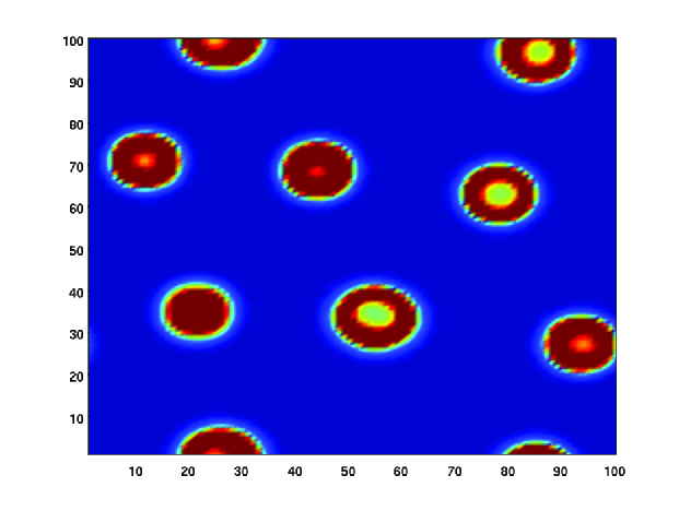
The numerical simulations provided in Section 5 suggest that for G>0𝐺0G>0 (for instance, G(s)=es𝐺𝑠superscript𝑒𝑠G(s)=e^{-s}) and bounded domain with periodic boundary conditions, the stationary solutions of (3.4) consist of one or more localized, but not compactly supported aggregates (clumps), see the bottom right panel of Fig. 5 and Fig. 7. However, we were not able to characterize these stationary aggregates analytically. Instead, we provide a few examples of other types of stationary solutions, posed either in the full space setting Ω=dΩsuperscript𝑑\Omega=\mathbb{R}^{d} or on a torus Ω=𝕋dΩsuperscript𝕋𝑑\Omega=\mathbb{T}^{d} with periodically extended W𝑊W. These examples are rather trivial, however, still provide an interesting insight into the relatively rich structure of the solutions of (3.4).

  • The most trivial type of stationary solution is the constant state ϱc>0italic-ϱ𝑐0\varrho\equiv c>0. Clearly, this has finite mass only if Ω=𝕋dΩsuperscript𝕋𝑑\Omega=\mathbb{T}^{d}.

  • If there exists an s0>0subscript𝑠00s_{0}>0 such that G(s)0𝐺𝑠0G(s)\equiv 0 for all ss0𝑠subscript𝑠0s\geq s_{0}, then any profile ϱitalic-ϱ\varrho such that ϱs0(ΩW(x)dx)1italic-ϱsubscript𝑠0superscriptsubscriptΩ𝑊𝑥differential-d𝑥1\varrho\geq s_{0}\left(\int_{\Omega}W(x)\,\mathrm{d}x\right)^{-1} almost everywhere on ΩΩ\Omega is a stationary solution to the distributional formulation (4.8). Indeed, such a solution satisfies Wϱs0𝑊italic-ϱsubscript𝑠0W\ast\varrho\geq s_{0}, so that G(Wϱ)0𝐺𝑊italic-ϱ0G(W\ast\varrho)\equiv 0. However, again, this solution has infinite mass if Ω=dΩsuperscript𝑑\Omega=\mathbb{R}^{d}.

  • If there exists an s0>0subscript𝑠00s_{0}>0 such that G(s)0𝐺𝑠0G(s)\equiv 0 for all ss0𝑠subscript𝑠0s\geq s_{0}, and, moreover, W𝑊W is continuous on ΩΩ\Omega, we construct the atomic measure

    ϱ(x)=i=1Nciδ(xxi)italic-ϱ𝑥superscriptsubscript𝑖1𝑁subscript𝑐𝑖𝛿𝑥subscript𝑥𝑖\displaystyle\varrho(x)=\sum_{i=1}^{N}c_{i}\delta(x-x_{i})

    for some N𝑁N\in\mathbb{N}, xiΩsubscript𝑥𝑖Ωx_{i}\in\Omega and ci>0subscript𝑐𝑖0c_{i}>0 such that ciW(0)>s0subscript𝑐𝑖𝑊0subscript𝑠0c_{i}W(0)>s_{0} for all i=1,,N𝑖1𝑁i=1,\dots,N. Then ϱitalic-ϱ\varrho is a distributional stationary solution to (4.8). Indeed, for any i=1,,N𝑖1𝑁i=1,\dots,N we have

    Wϱ(xi)=j=1NcjW(xixj)ciW(0)>s0.𝑊italic-ϱsubscript𝑥𝑖superscriptsubscript𝑗1𝑁subscript𝑐𝑗𝑊subscript𝑥𝑖subscript𝑥𝑗subscript𝑐𝑖𝑊0subscript𝑠0\displaystyle W\ast\varrho(x_{i})=\sum_{j=1}^{N}c_{j}W(x_{i}-x_{j})\geq c_{i}W(0)>s_{0}\,.

    By the continuity of W𝑊W and, consequently, Wϱ𝑊italic-ϱW\ast\varrho, we have Wϱ>s0𝑊italic-ϱsubscript𝑠0W\ast\varrho>s_{0} on some neighbourhood of xisubscript𝑥𝑖x_{i}. Therefore, G(Wϱ)0𝐺𝑊italic-ϱ0G(W\ast\varrho)\equiv 0 on some open set containing i=1Nxisuperscriptsubscript𝑖1𝑁subscript𝑥𝑖\bigcup_{i=1}^{N}x_{i} and, finally, G(Wϱ)ϱ0𝐺𝑊italic-ϱitalic-ϱ0G(W\ast\varrho)\varrho\equiv 0 everywhere on ΩΩ\Omega.

4.4 Linear stability analysis

In this section we perform a linear stability analysis of constant density states of the nonlinear diffusion equation (3.4). As discussed previously, we have constant steady state solutions either in the full-space setting Ω=dΩsuperscript𝑑\Omega=\mathbb{R}^{d} (however, with infinite mass), or on a bounded domain ΩdΩsuperscript𝑑\Omega\subset\mathbb{R}^{d} with periodic boundary conditions. Without loss of generality, we assume the normalization ΩW(x)dx=1subscriptΩ𝑊𝑥differential-d𝑥1\int_{\Omega}W(x)\,\mathrm{d}x=1. Let us make the perturbation ansatz ϱ=ϱ0+εϱ~italic-ϱsubscriptitalic-ϱ0𝜀~italic-ϱ\varrho=\varrho_{0}+\varepsilon\tilde{\varrho}, where ϱ0>0subscriptitalic-ϱ00\varrho_{0}>0 is a constant state such that G(ϱ0)>0𝐺subscriptitalic-ϱ00G(\varrho_{0})>0 and G(ϱ0)<0superscript𝐺subscriptitalic-ϱ00G^{\prime}(\varrho_{0})<0. Then Wϱ=ϱ0+εWϱ~𝑊italic-ϱsubscriptitalic-ϱ0𝜀𝑊~italic-ϱW\ast\varrho=\varrho_{0}+\varepsilon W\ast\tilde{\varrho} and assuming sufficient smoothness of G𝐺G, we have

G(Wϱ)2=G(ϱ0)2+2εG(ϱ0)G(ϱ0)Wϱ~+O(ε2).𝐺superscript𝑊italic-ϱ2𝐺superscriptsubscriptitalic-ϱ022𝜀𝐺subscriptitalic-ϱ0superscript𝐺subscriptitalic-ϱ0𝑊~italic-ϱ𝑂superscript𝜀2\displaystyle G(W\ast\varrho)^{2}=G(\varrho_{0})^{2}+2\varepsilon G(\varrho_{0})G^{\prime}(\varrho_{0})W\ast\tilde{\varrho}+O(\varepsilon^{2})\,.

Inserting the ansatz into (3.4) and collecting terms of order 𝒪(ε)𝒪𝜀\mathcal{O}(\varepsilon), we arrive at

ϱ~tG(ϱ0)2(G(ϱ0)Δϱ~+2G(ϱ0)ϱ0Δ(Wϱ~))=0.~italic-ϱ𝑡𝐺subscriptitalic-ϱ02𝐺subscriptitalic-ϱ0Δ~italic-ϱ2superscript𝐺subscriptitalic-ϱ0subscriptitalic-ϱ0Δ𝑊~italic-ϱ0\displaystyle\frac{\partial\tilde{\varrho}}{\partial t}-\frac{G(\varrho_{0})}{2}\left(G(\varrho_{0})\Delta\tilde{\varrho}+2G^{\prime}(\varrho_{0})\varrho_{0}\Delta(W\ast\tilde{\varrho})\right)=0\,.

Performing the Fourier transform, we obtain

ϱ^t+|ξ|2G(ϱ0)2(G(ϱ0)+2G(ϱ0)ϱ0W^)ϱ^=0,^italic-ϱ𝑡superscript𝜉2𝐺subscriptitalic-ϱ02𝐺subscriptitalic-ϱ02superscript𝐺subscriptitalic-ϱ0subscriptitalic-ϱ0^𝑊^italic-ϱ0\displaystyle\frac{\partial\hat{\varrho}}{\partial t}+|\xi|^{2}\frac{G(\varrho_{0})}{2}\left(G(\varrho_{0})+2G^{\prime}(\varrho_{0})\varrho_{0}\hat{W}\right)\hat{\varrho}=0\,, (4.9)

where we denoted ϱ^=ϱ^(t,ξ)^italic-ϱ^italic-ϱ𝑡𝜉\hat{\varrho}=\hat{\varrho}(t,\xi) the Fourier transform of ϱ~~italic-ϱ\tilde{\varrho}. Consequently, with the assumption G(ϱ0)>0𝐺subscriptitalic-ϱ00G(\varrho_{0})>0 and G(ϱ0)<0superscript𝐺subscriptitalic-ϱ00G^{\prime}(\varrho_{0})<0, those wavenumbers ξ𝜉\xi of ϱ~~italic-ϱ\tilde{\varrho} are stable for which

Re W^(ξ)<G(ϱ0)2G(ϱ0)ϱ00.Re ^𝑊𝜉𝐺subscriptitalic-ϱ02superscript𝐺subscriptitalic-ϱ0subscriptitalic-ϱ00\displaystyle\mbox{Re }\hat{W}(\xi)<-\frac{G(\varrho_{0})}{2G^{\prime}(\varrho_{0})\varrho_{0}}\geq 0\,. (4.10)

Since WL1(d)𝑊superscript𝐿1superscript𝑑W\in L^{1}(\mathbb{R}^{d}), we have W^C0(d)^𝑊superscript𝐶0superscript𝑑\hat{W}\in C^{0}(\mathbb{R}^{d}), and, therefore, all wavenumbers of ϱ~~italic-ϱ\tilde{\varrho} larger than a certain threshold will be stable. On the other hand, wavenumbers violating (4.10) will lead to pattern formation, as we show in our numerical examples, Section 5. Moreover, a quick inspection of (4.9) leads to the expectation that the stable high wavenumbers will be smoothed-out on a faster time scale, compared to the slower emergence of patterns due to the unstable lower wavenumbers. Finally, considering the scalings Wr(x):=rdW1(x/r)assignsubscript𝑊𝑟𝑥superscript𝑟𝑑subscript𝑊1𝑥𝑟W_{r}(x):=r^{-d}W_{1}(x/r) of a fixed kernel W1L1(d)subscript𝑊1superscript𝐿1superscript𝑑W_{1}\in L^{1}(\mathbb{R}^{d}), we have Wr^(ξ)=W1^(rξ)^subscript𝑊𝑟𝜉^subscript𝑊1𝑟𝜉\hat{W_{r}}(\xi)=\hat{W_{1}}(r\xi) and, therefore, we expect that the wavelength of the patterns (size of aggregates) will scale with r𝑟r. This can be as well clearly observed in our numerical examples.

It is interesting to consider the formal extremal case W=δ0𝑊subscript𝛿0W=\delta_{0}, i.e., Wϱ~=ϱ~𝑊~italic-ϱ~italic-ϱW\ast\tilde{\varrho}=\tilde{\varrho}. Then W^1^𝑊1\hat{W}\equiv 1 and we conclude that the constant state ϱ0subscriptitalic-ϱ0\varrho_{0} is stable if and only if

(G(ϱ0)2ϱ0)=G(ϱ0)2+2G(ϱ0)G(ϱ0)ϱ0>0.superscript𝐺superscriptsubscriptitalic-ϱ02subscriptitalic-ϱ0𝐺superscriptsubscriptitalic-ϱ022𝐺subscriptitalic-ϱ0superscript𝐺subscriptitalic-ϱ0subscriptitalic-ϱ00\displaystyle(G(\varrho_{0})^{2}\varrho_{0})^{\prime}=G(\varrho_{0})^{2}+2G(\varrho_{0})G^{\prime}(\varrho_{0})\varrho_{0}>0\,. (4.11)

In fact, violation of (4.11) with W=δ0𝑊subscript𝛿0W=\delta_{0} leads to an ill-posed problem, since then (3.4) looks like a backward heat equation, which can be seen if we expand the derivatives and write it in the Fokker-Planck form as

ϱt=12(G(ϱ)[2G(ϱ)ϱ+G(ϱ)]ϱ).italic-ϱ𝑡12𝐺italic-ϱdelimited-[]2superscript𝐺italic-ϱitalic-ϱ𝐺italic-ϱitalic-ϱ\displaystyle\frac{\partial\varrho}{\partial t}=\frac{1}{2}\nabla\cdot\left(G(\varrho)[2G^{\prime}(\varrho)\varrho+G(\varrho)]\nabla\varrho\right)\,. (4.12)

The equation is parabolic (and thus well-posed) only if the diffusivity 2G(ϱ)G(ϱ)ϱ+G2(ϱ)2𝐺italic-ϱsuperscript𝐺italic-ϱitalic-ϱsuperscript𝐺2italic-ϱ2G(\varrho)G^{\prime}(\varrho)\varrho+G^{2}(\varrho) is strictly positive, which is our stability condition (4.11). Therefore, only imposing an initial condition ϱ0subscriptitalic-ϱ0\varrho_{0} uniformly satisfying (4.11) leads to a well-posed diffusion equation for all t0𝑡0t\geq 0, since (4.11) is preserved due to the maximum principle. On the other hand, if G>0𝐺0G>0, the nonlocality WL1(d)𝑊superscript𝐿1superscript𝑑W\in L^{1}(\mathbb{R}^{d}) always stabilizes the equation in the sense of (4.10). Indeed, writing it in the Fokker-Planck form

ϱt=12(Individualbasedandmeanfieldmodellingofdirectaggregation[2G(Wϱ)G(Wϱ)Wϱ]ϱ+G2(Wϱ)ϱ),italic-ϱ𝑡12𝐼𝑛𝑑𝑖𝑣𝑖𝑑𝑢𝑎𝑙𝑏𝑎𝑠𝑒𝑑𝑎𝑛𝑑𝑚𝑒𝑎𝑛𝑓𝑖𝑒𝑙𝑑𝑚𝑜𝑑𝑒𝑙𝑙𝑖𝑛𝑔𝑜𝑓𝑑𝑖𝑟𝑒𝑐𝑡𝑎𝑔𝑔𝑟𝑒𝑔𝑎𝑡𝑖𝑜𝑛delimited-[]2𝐺𝑊italic-ϱsuperscript𝐺𝑊italic-ϱ𝑊italic-ϱitalic-ϱsuperscript𝐺2𝑊italic-ϱitalic-ϱ\displaystyle\frac{\partial\varrho}{\partial t}=\frac{1}{2}\nabla\cdot\left(Individualbasedandmean-fieldmodellingofdirectaggregation\left[2G(W\ast\varrho)G^{\prime}(W\ast\varrho)\nabla W\ast\varrho\right]\varrho+G^{2}(W\ast\varrho)\nabla\varrho\right)\,,

we see that the second-order term appears with the positive diffusivity G2(Wϱ)superscript𝐺2𝑊italic-ϱG^{2}(W\ast\varrho). The first-order term describes then the transport of ϱitalic-ϱ\varrho along the generalized gradient Wϱ𝑊italic-ϱ\nabla W\ast\varrho and is responsible for the aggregative effect.

Clearly, the ill-posedness of (4.12) can be avoided by merely introducing a nonlocality in the first-order transport term, while the diffusivity may stay local (and possibly degenerate). Such a model was derived and studied in [30], which with our notation is written as

ϱt=(ϱWϱ+ϱ2ϱ).italic-ϱ𝑡italic-ϱ𝑊italic-ϱsuperscriptitalic-ϱ2italic-ϱ\displaystyle\frac{\partial\varrho}{\partial t}=\nabla\cdot\left(-\varrho\nabla W\ast\varrho+\varrho^{2}\nabla\varrho\right)\,.

This equation was constructed as a model for biological aggregations in which individuals experience long-range social attraction and short range dispersal. Let us note that here, in contrast to our model, the diffusivity is an increasing function of the density ϱitalic-ϱ\varrho. In [30] it was shown that it produces strongly nonlinear states with compact support and steep edges that correspond to localized biological aggregations, or clumps. Similarly as can be observed in our numerical simulations in Section 5, these clumps are approached through a dynamic coarsening process.

Another insight into the stabilizing effect of the nonlocality is provided by the introduction of a formal expansion of W𝑊W. Taking W𝑊W as the standard mollifier and Wε(s):=εdW(s/ε)assignsubscript𝑊𝜀𝑠superscript𝜀𝑑𝑊𝑠𝜀W_{\varepsilon}(s):=\varepsilon^{-d}W(s/\varepsilon), such that Wεδ0subscript𝑊𝜀subscript𝛿0W_{\varepsilon}\to\delta_{0} as ε0𝜀0\varepsilon\to 0, we expand

Wεϱsubscript𝑊𝜀italic-ϱ\displaystyle W_{\varepsilon}\ast\varrho =\displaystyle= εddW(xyε)ϱ(y)dysuperscript𝜀𝑑subscriptsuperscript𝑑𝑊𝑥𝑦𝜀italic-ϱ𝑦differential-d𝑦\displaystyle\varepsilon^{-d}\int_{\mathbb{R}^{d}}W\left(\frac{x-y}{\varepsilon}\right)\varrho(y)\,\mathrm{d}y
=\displaystyle= dW(z)ϱ(x+εz)dzsubscriptsuperscript𝑑𝑊𝑧italic-ϱ𝑥𝜀𝑧differential-d𝑧\displaystyle\int_{\mathbb{R}^{d}}W(-z)\varrho(x+\varepsilon z)\,\mathrm{d}z
=\displaystyle= dW(z)(ϱ(x)+εϱ(x)z+12ε2zt2ϱ(x)z)dz+𝒪(ε3).subscriptsuperscript𝑑𝑊𝑧italic-ϱ𝑥𝜀italic-ϱ𝑥𝑧12superscript𝜀2superscript𝑧𝑡superscript2italic-ϱ𝑥𝑧differential-d𝑧𝒪superscript𝜀3\displaystyle\int_{\mathbb{R}^{d}}W(-z)\left(\varrho(x)+\varepsilon\nabla\varrho(x)z+\frac{1}{2}\varepsilon^{2}z^{t}\nabla^{2}\varrho(x)z\right)\,\mathrm{d}z+\mathcal{O}(\varepsilon^{3})\,.

Now, due to the symmetry W(z)=W(z)𝑊𝑧𝑊𝑧W(-z)=W(z) and the normalization dW(z)dz=1subscriptsuperscript𝑑𝑊𝑧differential-d𝑧1\int_{\mathbb{R}^{d}}W(z)\,\mathrm{d}z=1, we have

Wεϱ=ϱ+ε22βΔϱ+𝒪(ε4),subscript𝑊𝜀italic-ϱitalic-ϱsuperscript𝜀22𝛽Δitalic-ϱ𝒪superscript𝜀4\displaystyle W_{\varepsilon}\ast\varrho=\varrho+\frac{\varepsilon^{2}}{2}\beta\Delta\varrho+\mathcal{O}(\varepsilon^{4})\,,

where the constant β>0𝛽0\beta>0 is such that dW(z)zizjdz=βδijsubscriptsuperscript𝑑𝑊𝑧subscript𝑧𝑖subscript𝑧𝑗differential-d𝑧𝛽subscript𝛿𝑖𝑗\int_{\mathbb{R}^{d}}W(z)z_{i}z_{j}\,\mathrm{d}z=\beta\delta_{ij}. Inserting this into (3.4), we obtain

tϱsubscript𝑡italic-ϱ\displaystyle\partial_{t}\varrho =\displaystyle= 12Δ(G(ϱ+ε22βΔϱ+𝒪(ε4))2ϱ)12Δ𝐺superscriptitalic-ϱsuperscript𝜀22𝛽Δitalic-ϱ𝒪superscript𝜀42italic-ϱ\displaystyle\frac{1}{2}\Delta\left(G\left(\varrho+\frac{\varepsilon^{2}}{2}\beta\Delta\varrho+\mathcal{O}(\varepsilon^{4})\right)^{2}\varrho\right)
=\displaystyle= 12Δ(G(ϱ)2ϱ+ε2βG(ϱ)G(ϱ)ϱΔϱ)+𝒪(ε4).12Δ𝐺superscriptitalic-ϱ2italic-ϱsuperscript𝜀2𝛽𝐺italic-ϱsuperscript𝐺italic-ϱitalic-ϱΔitalic-ϱ𝒪superscript𝜀4\displaystyle\frac{1}{2}\Delta\left(G(\varrho)^{2}\varrho+\varepsilon^{2}\beta G(\varrho)G^{\prime}(\varrho)\varrho\Delta\varrho\right)+\mathcal{O}(\varepsilon^{4})\,.

Up to the terms of fourth order in ε𝜀\varepsilon, this is a Cahn-Hilliard-type equation which is well-posed for every ε>0𝜀0\varepsilon>0 since the term ε2βG(ϱ)G(ϱ)ϱsuperscript𝜀2𝛽𝐺italic-ϱsuperscript𝐺italic-ϱitalic-ϱ\varepsilon^{2}\beta G(\varrho)G^{\prime}(\varrho)\varrho is strictly negative if G(ϱ)>0𝐺italic-ϱ0G(\varrho)>0 and G(ϱ)<0superscript𝐺italic-ϱ0G^{\prime}(\varrho)<0. However, if ε=0𝜀0\varepsilon=0, i.e. W=δ0𝑊subscript𝛿0W=\delta_{0}, this regularizing effect is lost.

5 Numerical examples

In this section we present numerical examples for the first and second-order individual based models (2.2), (2.4)–(2.5) in 2D, the first-order mean-field limit (3.4) in 1D and 2D and the second-order mean-field limit (3.5) in 1D with 1D velocity.

5.1 The first-order individual based model (2.2)

We consider a system consisting of N=400𝑁400N=400 individuals in a 2D domain Ω=(0,1)×(0,1)Ω0101\Omega=(0,1)\times(0,1) with periodic boundary conditions. The initial positions are generated randomly and independently for each individual from the uniform distribution on ΩΩ\Omega; we took the same initial condition for all the three experiments below. We choose W(x)=w(|x|)𝑊𝑥𝑤𝑥W(x)=w(|x|) with w𝑤w the characteristic function of the interval [0,R]0𝑅[0,R], corresponding to the sampling radius R𝑅R, and for R𝑅R we take the values 0.0250.0250.025 (Fig. 1), 0.050.050.05 (Fig. 2) and 0.10.10.1 (Fig. 3). For G𝐺G we make the choice G(s)=exp(s/3)𝐺𝑠𝑠3G(s)=\exp(-s/3). The system of stochastic differential equations (2.2) is integrated in time using the Euler-Mayurama scheme with time-step length t=103𝑡superscript103t=10^{-3}. We used the linear stability analysis in Section 5 to make the “right” choice of G𝐺G, such that we could observe pattern formation. Indeed, if G𝐺G decreases too quickly, the system will “freeze” immediately, before any aggregates could be formed; on the other hand, if G𝐺G does not decrease fast enough, the system is “overheated” and does not allow aggregates to persist.

In Figs. 1, 2 and 3 we observe that with a smaller sampling radius R𝑅R, a larger number of small aggregates is created on a faster time scale. The choice R=0.1𝑅0.1R=0.1 (Fig.3) leads to creation of one sigle aggregate. This aggregate is approximately ring-shaped, with higher density of particles around the circumference and lower density in the middle. This can be explained by the fact that the aggregate grows by “capturing” particles from its neighborhood, and once a particle is captured, its mobility is greatly reduced, so that it only slowly makes its way towards the center of the aggregate. Let us also mention that the right-most panels in Figs. 13 present quasi-steady states, where the aggregates are in a dynamic equilibrium with a very few free-running particles. However, on a very long time scale, the smaller aggregates typically disintegrate and their particles are caught by the larger ones. Such a coarsening behavior is typical to diffusive aggregation systems, as for instance the Cahn-Hilliard equation, or the nonlocal continuum model of [30].
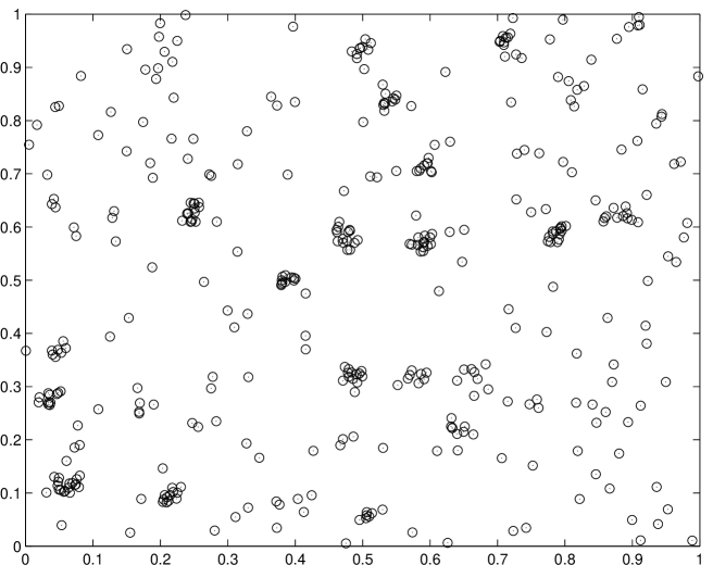
Refer to caption
Refer to caption
Refer to caption
t=0.1 t=0.2 t=1.7
Figure 1: The first-order individual based model with N=400𝑁400N=400 agents and sampling radius R=0.025𝑅0.025R=0.025, subject to a random initial condition.
Refer to caption
Refer to caption
Refer to caption
t=0.1 t=0.25 t=0.7
Figure 2: The first-order individual based model with N=400𝑁400N=400 agents and sampling radius R=0.05𝑅0.05R=0.05, subject to a random initial condition.
Refer to caption
Refer to caption
Refer to caption
t=1.5 t=2.0 t=8.3
Figure 3: The first-order individual based model with N=400𝑁400N=400 agents and sampling radius R=0.1𝑅0.1R=0.1, subject to a random initial condition.

5.2 The second-order individual based model (2.4)–(2.5)

Generally, the behavior of the second-order individual based model is very similar to this of the first-order one, at least if we do not impose a restricted cone of vision (i.e., W𝑊W in (2.3) does not depend on v𝑣v). Indeed, with a suitable choice of parameters, one again observes the formation of quasi-stable aggregates, whose number and size depend on the sampling radius. The most striking difference with respect to the first-order model is that the movement of the agents is smoother (their velocities are continuous) and the shape of the aggregates is more complex (we observed emergence of ellipsoidal aggregates, instead of the almost-circular ones in the first-order model).

The situation becomes slightly more interesting if we consider a restricted cone of vision - we choose 180°, such that W(x,v)=w(|x|,xv|x||v|)𝑊𝑥𝑣𝑤𝑥𝑥𝑣𝑥𝑣W(x,v)=w\left(|x|,\frac{x\cdot v}{|x||v|}\right) with w(s,z)=χ[0,R](s)χ[0,1](z)𝑤𝑠𝑧subscript𝜒0𝑅𝑠subscript𝜒01𝑧w(s,z)=\chi_{[0,R]}(s)\chi_{[0,1]}(z). The sampling radius is chosen as R=0.05𝑅0.05R=0.05. Again, we simulate with N=400𝑁400N=400 individuals in a 2D domain Ω=(0,1)×(0,1)Ω0101\Omega=(0,1)\times(0,1) with periodic boundary conditions, and G(s)=exp(s/3)𝐺𝑠𝑠3G(s)=\exp(-s/3). For H𝐻H we set the constant H2𝐻2H\equiv 2. The system of stochastic differential equations (2.4)–(2.5) is integrated in time using the Euler-Mayurama scheme with time-step length t=103𝑡superscript103t=10^{-3}. The initial positions of the agents are generated randomly in the same way as for the first-order model, while their initial velocities are generated independently and randomly from the 2D normalized Gaussian distribution. Three snapshots of the evolution of the system are shown in Fig. 4, the velocities being marked by the linear elements for each individual. The right-most panel in Fig. 4 shows the quasi-steady state with two aggregates formed, in dynamic equilibrium with the “free-running” individuals. It is obvious that, compared to the previous simulations, the aggregates are less densely packed and their shapes are less circular. Also, the portion of the “free-running” particles is much higher, which clearly is an effect of the restricted cone of vision (the captured particles can leave the aggregate more easily).
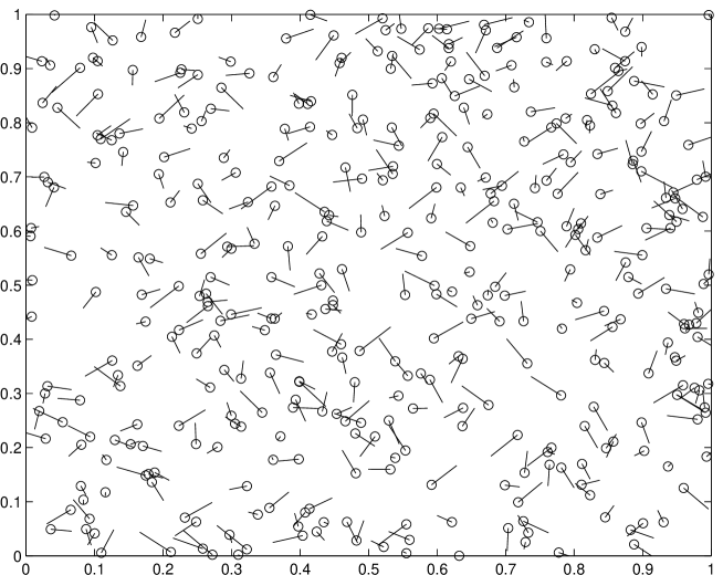
Refer to caption
Refer to caption
Refer to caption
t=0.000 t=0.044 t=0.104
Figure 4: The second-order individual based model with N=400𝑁400N=400 agents, sampling radius R=0.05𝑅0.05R=0.05 and 180° cone of vision, subject to a random initial condition.

5.3 The first-order mean-field model (3.4) in 1D

We simulated the first-order mean-field model (3.4) in the 1D periodic domain (0,1)01(0,1), using semi-implicit finite difference discretization for the space variable and first-order forward Euler method for the time variable. The space grid consisted of 200200200 equidistant points, the time step was 104superscript10410^{-4}. As before, we chose W(x)=w(|x|)𝑊𝑥𝑤𝑥W(x)=w(|x|) with w𝑤w the characteristic function of the interval [0,0.1]00.1[0,0.1], and G(s)=exp(s/3)𝐺𝑠𝑠3G(s)=\exp(-s/3). We imposed a random initial condition for ϱitalic-ϱ\varrho, generated such that for every grid point a random number from the uniform distribution in [0,1]01[0,1] has been drawn. Snapshots of the evolution are shown in Fig. 5. We observe that quite a strong smoothing effect takes place on the fast time-scale (first row in Fig. 5), while aggregation takes place on a time-scale approximately one order of magnitude slower (second row); this is explained with the stability analysis in Section 4.4. First, two aggregates of different sizes are created, however, both of them are unstable - the smaller one is smoothed out, while the larger grows further, until the steady state is reached (lower right panel). Observe also the characteristic “fork”-like shape of the profile in the lower mid panel (t=2.65𝑡2.65t=2.65), which is due to the mass arriving from the neighbourhood with higher diffusivity than the diffusivity in the middle of the profile; compare also with the ring-shaped aggregate in the right panel of Fig. 2. However, this fork-like structure is eventually also smoothed out, to finally obtain the steady profile. Let us note that the steady aggregate, although well localized, is not compactly supported, i.e., the profile has positive density everywhere on [0,1]01[0,1].

Refer to caption
Refer to caption
Refer to caption
t=0.0000 t=0.0008 t=0.1300
Refer to caption
Refer to caption
Refer to caption
t=0.8500 t=2.6500 t=11.0500
Figure 5: The first-order mean-field model in a periodic 1D setting with random initial condition (upper left panel). Steady state was reached at t11similar-to-or-equals𝑡11t\simeq 11 (lower right panel).

5.4 The first-order mean-field model (3.4) in 2D

We simulated the first-order mean-field model (3.4) in the 2D periodic domain (0,1)2superscript012(0,1)^{2}, using the same type of discretization as in the 1D case. The space grid consisted of 100×100100100100\times 100 equidistant points, the time step was 104superscript10410^{-4}. We chose the sampling radius R=0.07𝑅0.07R=0.07, i.e., W(x)=χ[0,0.7](|x|)𝑊𝑥subscript𝜒00.7𝑥W(x)=\chi_{[0,0.7]}(|x|), and G(s)=exp(s/3)𝐺𝑠𝑠3G(s)=\exp(-s/3). Snapshots of the evolution are shown in Fig. 6. Starting again from a random initial condition, we observed a rapid formation of approximately ring-shaped pre-aggregates, which eventually turn into an almost regular pattern of well localized (but not compactly supported) clumps. However, the smaller aggregates may be unstable and diffusively disintegrate, and their mass is absorbed by their neighbors, as shown on the lower right panel of Fig. 6. Finally, in Fig. 7 we present examples of patterns produced with the sampling radii R=0.6𝑅0.6R=0.6 (left panel) and R=0.11𝑅0.11R=0.11 (right panel).

Refer to caption
Refer to caption
t=0.000 t=0.005
Refer to caption
Refer to caption
t=0.900 t=0.950
Figure 6: The first-order mean-field model in a periodic 2D setting with random initial condition (upper left panel). After the initial rapid smoothing of the high-frequency components, several ring-shaped structures are created (upper right panel), which eventually turn into an almost regular pattern of well localized aggregates (lower left panel). However, the smaller aggregates may be unstable and diffusively disintegrate, and their mass is absorbed by their neighbors, (lower right panel).
Refer to caption
Refer to caption
R=0.06 R=0.11
Figure 7: An example of patterns produced by the first-order mean-field model in a periodic 2D setting with the sampling radii R=0.6𝑅0.6R=0.6 (left panel) and R=0.11𝑅0.11R=0.11 (right panel).

5.5 The second-order mean-field model (3.5)

We conclude this section with simulations of the second-order mean-field model (3.5) in 1D. The spatial domain Ω=[a,b]Ω𝑎𝑏\Omega=[a,b] is discretized using an equidistant mesh xi=a+iΔxsubscript𝑥𝑖𝑎𝑖Δ𝑥x_{i}=a+i\Delta x, the velocity domain V=[vmin,vmax]𝑉subscript𝑣subscript𝑣V=[v_{\min},v_{\max}] at grid points vj=vmin+jΔvsubscript𝑣𝑗subscript𝑣𝑗Δ𝑣v_{j}=v_{\min}+j\Delta v. The time step ΔtΔ𝑡\Delta t satisfies the CFL condition for vmaxsubscript𝑣v_{\max}, i.e., Δt=Δx|vmax|Δ𝑡Δ𝑥subscript𝑣\Delta t=\frac{\Delta x}{\lvert v_{\max}\rvert}. The numerical scheme is based on a splitting method: Given an initial datum f(x,v,0)=f0(x,v)𝑓𝑥𝑣0subscript𝑓0𝑥𝑣f(x,v,0)=f_{0}(x,v), we split the system at every time tk=kΔtsubscript𝑡𝑘𝑘Δ𝑡t_{k}=k\Delta t into the following steps:

  1. 1.

    Solve transport equation in x𝑥x

    ft+vixf𝑓𝑡subscript𝑣𝑖subscript𝑥𝑓\displaystyle\frac{\partial f}{\partial t}+v_{i}\cdot\nabla_{x}f =0,absent0\displaystyle=0, (5.1)

    subject to periodic boundary conditions on ΩΩ\Omega, for every visubscript𝑣𝑖v_{i} on the time interval t[tk,tk+12Δt]𝑡subscript𝑡𝑘subscript𝑡𝑘12Δ𝑡t\in[t_{k},t_{k}+\frac{1}{2}\Delta t], using an upwind scheme with the superbee flux limiter.

  2. 2.

    Starting with the solution of the transport equation (5.1), solve

    ft=v(H(Wf)vf+12v(G(Wf)2f)),𝑓𝑡subscript𝑣𝐻𝑊𝑓𝑣𝑓12subscript𝑣𝐺superscript𝑊𝑓2𝑓\displaystyle\frac{\partial f}{\partial t}=\nabla_{v}\cdot\left(H(W\circledast f)vf+\frac{1}{2}\nabla_{v}(G(W\circledast f)^{2}f)\right), (5.2)

    with no flux boundary conditions on V𝑉V, on the time interval [tk,tk+1]subscript𝑡𝑘subscript𝑡𝑘1[t_{k},t_{k+1}], using a semi-implicit time discretization.

  3. 3.

    Finally solve (5.1) using the solution of (5.2) for another half time step 12Δt12Δ𝑡\frac{1}{2}\Delta t.

We set the computational domain to Ω=[0,1]Ω01\Omega=[0,1], the velocity domain to V=[1,1]𝑉11V=[-1,1] and the mesh sizes to Δx=102Δ𝑥superscript102\Delta x=10^{-2} and Δv=2×10²Δ𝑣2superscript102\Delta v=2\times 10^{-2}. We choose similar conditions as in the individual based model, i.e. a limited cone of vision W(x,v)=w(|x|,xv|x||v|)𝑊𝑥𝑣𝑤𝑥𝑥𝑣𝑥𝑣W(x,v)=w(\lvert x\rvert,\frac{x\cdot v}{\lvert x\rvert\lvert v\rvert}) with w(s,z)=χ[0.R](s)χ[0,1](z)𝑤𝑠𝑧subscript𝜒delimited-[]formulae-sequence0𝑅𝑠subscript𝜒01𝑧w(s,z)=\chi_{[0.R]}(s)\chi_{[0,1]}(z). The sampling radius is set to R=0.07𝑅0.07R=0.07, G(s)=exp(2s)𝐺𝑠2𝑠G(s)=\exp(-2s) and H2𝐻2H\equiv 2. The initial datum corresponds to a small perturbation of a uniform distribution with mass one. Snapshots of the evolution of the particle distribution density f(t,x,v)𝑓𝑡𝑥𝑣f(t,x,v) and the mass density ρ(t,x)𝜌𝑡𝑥\rho(t,x) at different times are depicted in Fig. 8. We observe a fast smoothing of f(t,x,v)𝑓𝑡𝑥𝑣f(t,x,v) in time and a subsequent formation of a stable aggregate.

If we decrease the sampling radius to R=0.03𝑅0.03R=0.03, two separate aggregates form, see Fig. 9. Again, we observe that with a smaller sampling radius the aggregation happens on a faster time scale.
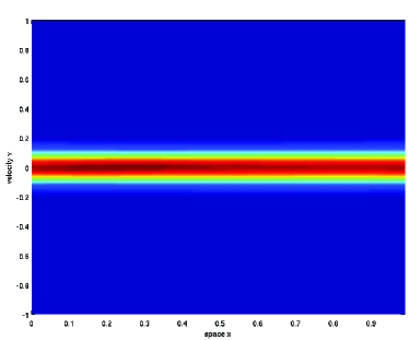
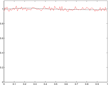
Refer to caption
(a) Particle distribution function f(t,x,v)𝑓𝑡𝑥𝑣f(t,x,v) at t=4𝑡4t=4
Refer to caption
(b) Mass density ρ(t,x)𝜌𝑡𝑥\rho(t,x) at t=4𝑡4t=4
Refer to caption
(c) Particle distribution function f(t,x,v)𝑓𝑡𝑥𝑣f(t,x,v) at t=8𝑡8t=8
Refer to caption
(d) Mass density ρ(t,x)𝜌𝑡𝑥\rho(t,x) at t=8𝑡8t=8
Refer to caption
(e) Particle distribution function f(t,x,v)𝑓𝑡𝑥𝑣f(t,x,v) at t=20𝑡20t=20
Refer to caption
(f) Mass density ρ(t,x)𝜌𝑡𝑥\rho(t,x) at t=20𝑡20t=20
Figure 8: Second order model with limited vision and R=0.07𝑅0.07R=0.07; the red line in the left column indicates the initial datum.
Refer to caption
(a) Particle distribution function f(t,x,v)𝑓𝑡𝑥𝑣f(t,x,v) at t=4𝑡4t=4
Refer to caption
(b) Mass density ρ(t,x)𝜌𝑡𝑥\rho(t,x) at t=4𝑡4t=4
Refer to caption
(c) Particle distribution function f(t,x,v)𝑓𝑡𝑥𝑣f(t,x,v) at t=8𝑡8t=8
Refer to caption
(d) Mass density ρ(t,x)𝜌𝑡𝑥\rho(t,x) at t=8𝑡8t=8
Refer to caption
(e) Particle distribution function f(t,x,v)𝑓𝑡𝑥𝑣f(t,x,v) at t=20𝑡20t=20
Refer to caption
(f) Mass density ρ(t,x)𝜌𝑡𝑥\rho(t,x) at t=20𝑡20t=20
Figure 9: Second order model with limited vision and R=0.03𝑅0.03R=0.03; the red line in the left column indicates the initial datum.

Acknowledgment: JH acknowledges the hospitality of the Faculty of Mathematics, University of Münster during his stay, where the work leading to this paper has been initiated. MTW acknowledges financial support from the Austrian Science Foundation (FWF) via the Hertha Firnberg project T456-N23 and the Award KUK-I1-006-43 by the King Abdullah University of Science and Technology (KAUST).

References

  • [1] K. Anguige, C. Schmeiser: A one-dimensional model of cell diffusion and aggregation, incorporating volume filling and cell-to-cell adhesion. J. Math. Biology (2009), pp.
  • [2] B. Briscoe, M. Lewis and S. Parrish: Home range formation in wolves due to scent marking. Bulletin of Mathematical Biology 64 (2002) 64, 261–284.
  • [3] M. Burger: Nonstandard BBGKY hierarchies. Preprint, 2011.
  • [4] H. Brezis, Analyse fonctionelle, Dunod, Paris, 1999.
  • [5] L. C. Evans, Partial Differential Equations,1998, American Mathematical Society, Providence, Rhode Island.
  • [6] P. Grindrod: Models of individual aggregation in single and multispecies communities. J. Math. Biol. 26 (1988), pp. 651–660.
  • [7] D. Grünbaum and A. Okubo: Modelling social animal aggregations. In: S. A. Levin (Ed.), Frontiers of Theoretical Biology. Vol. 100 of Lecture Notes in Biomathematics (1994), Springer-Verlag.
  • [8] E. Hernández-García and C. López: Clustering, advection, and patterns in a model of population dynamics with neighborhood-dependent rates. Phys. Rev. E 70 (2004), pp. 016216.
  • [9] R. Jeanson, S. Blanco, R. Fournier, J.-L. Deneubourg, V. Fourcassié and G. Theraulaz: A model of animal movements in a bounded space, Journal of Theoretical Biology 225 (2003), pp. 443–451.
  • [10] R. Jeanson, C. Rivault, J.-L. Deneubourg, S. Blanco, R. Fournier, C. Jost and G. Theraulaz: Self-organised aggregation in cockroaches, Animal Behaviour 69 (2005), pp. 169–180.
  • [11] C. Jost, R. Jeanson, J. Gautrais, B.-R. Bengoudifa, G. Theraulaz: Sensitivity of cockroach aggregation to individual and external parameters. Preprint, 2011.
  • [12] K. Kawasaki: Diffusion and the formation of spatial distribution. Mathematical Sciences 16 (1978), 47–52.
  • [13] E. F. Keller and L. A. Segel: Initiation of slime mold aggregation viewed as an instability. J. Theoret. Biol. 26 (1970), pp. 399–415.
  • [14] J. Krause and G. Ruxton: Living in groups. Oxford University Press, 2002.
  • [15] J. Krebs and N. Davies (eds.): Behavioural Ecology: An Evolutionary Approach. Sinauer, Sunderland Massachussetts, 1984.
  • [16] C. López: Self-propelled nonlinearly diffusing particles: Aggregation and continuum description. Phys. Rev. E 72 (2005), pp. 061109.
  • [17] C. López: Macroscopic description of particle systems with nonlocal density-dependent diffusivity. Phys. Rev. E 74 (2006), pp. 012102.
  • [18] P. Maini, L. Malaguti, C. Marcelli and S. Matucci: Diffusion-aggregation processes with monostable reaction terms. Discrete and Continuous Dynamical Systems Series B, 6 (5), 2006, 1175–1189.
  • [19] M. Mimura and M. Yamaguti: Pattern formation in interacting and diffusing systems in population biology. Advances in Biophysics 15 (1982), pp. 19–65.
  • [20] A. Mogilner and L. Edelstein-Keshet: A non-local model for a swarm. J. Math. Biol. 38 (1999), 534–570.
  • [21] J. Murray: Mathematical Biology. Springer, 2001.
  • [22] A. Okubo: Diffusion and Ecological Problems: Mathematical Models. Springer Verlag, 1980.
  • [23] V. Padrón: Aggregation on a Nonlinear Parabolic Functional Diferential Equation. Divulgaciones Matemáticas v. 6, No. 2 (1998), 149–164.
  • [24] V. Padrón: Effect of aggregation on population recovery modeled by a forward-backward pseudoparabolic equation. Trans. Amer. Math. Soc. 356 (2004), 2739–2756.
  • [25] F. Sánchez-Garduño, P. Maini and J. Pérez-Velázquez: A non-linear degenerate equation for direct aggregation and traveling wave dynamics. Discrete and Continuous Dynamical Systems Series B, 13 (2), 2010, pp. 455–487.
  • [26] M. Rust, J. Owens and D. Reierson: Understanding and controlling the german cockroach. Oxford University Press, 1995.
  • [27] M. J. Schnitzer: Theory of continuum random walker and application to chemotaxis. Phys. Rev. E 48 (1993), pp. 2553–2568.
  • [28] J. Simon: Compact sets in the space Lp(0,T;B)superscript𝐿𝑝0𝑇𝐵L^{p}(0,T;B). Ann. Mat. Pure Appl. IV (146), 1987, pp. 65-96.
  • [29] J. Skellam: Random dispersal in theoretical populations. Biometrika 38 (1951), 196–218.
  • [30] C. Topaz, A. Bertozzi and M. Lewis: A nonlocal continuum model for biological aggregation.
  • [31] P. Turchin: Population Consequences of Aggregative Movement. J. of Animal Ecology, Vol. 58, No. 1 (1989), pp. 75–100.
  • [32] P. Turchin, P. Kareiva: Aggregation in Aphis varians: an effective strategy for reducing predation risk. Ecology 70 (1989), pp. 1008-1016.