Weighted KS Statistics for Inference on Conditional Moment Inequalities

Abstract

This paper proposes confidence regions for the identified set in conditional moment inequality models using Kolmogorov-Smirnov statistics with a truncated inverse variance weighting with increasing truncation points. The new weighting differs from those proposed in the literature in two important ways. First, confidence regions based on KS tests with the weighting function I propose converge to the identified set at a faster rate than existing procedures based on bounded weight functions in a broad class of models. This provides a theoretical justification for inverse variance weighting in this context, and contrasts with analogous results for conditional moment equalities in which optimal weighting only affects the asymptotic variance. Second, the new weighting changes the asymptotic behavior, including the rate of convergence, of the KS statistic itself, requiring a new asymptotic theory in choosing the critical value, which I provide. To make these comparisons, I derive rates of convergence for the confidence regions I propose along with new results for rates of convergence of existing estimators under a general set of conditions. A series of examples illustrates the broad applicability of the conditions. A monte carlo study examines the finite sample behavior of the confidence regions.

1 Introduction

This paper proposes methods for inference in conditional moment inequality models and derives new relative efficiency results for these models to show that these methods are more efficient than available methods in a certain precise sense. Formally, these models are defined by a restriction of the form $E_{P}(m(W_{i},\theta)|X_{i})\geq 0$ almost surely. Here, $m$ is a known parametric function, which may be vector valued (in which case the inequality is interpreted as elementwise). This setup includes many models commonly used in econometrics, including regression models with endogenously censored or missing data, selection models, and certain models of firm and consumer behavior.

The problem is to perform inference on the identified set

$$\Theta_{0}(P)\equiv\{\theta|E_{P}(m(W_{i},\theta)|X_{i})\geq 0\text{ a.s.}\}$$

given a sample $(X_{1},W_{1}),\ldots,(X_{n},W_{n})$ from $P$. This paper proposes confidence regions $\mathcal{C}_{n}$ that satisfy

$$\liminf_{n\to\infty}\inf_{P\in\mathcal{P}}P(\Theta_{0}(P)\subseteq\mathcal{C}_{n})\geq 1-\alpha$$ (1)

for classes of probability distributions $\mathcal{P}$ restricted only by mild regularity conditions. For these confidence regions and several confidence regions available in the literature satisfying this requirement, I derive rates of convergence of $\mathcal{C}_{n}$ to $\Theta_{0}(P)$. The results give sequences $a_{n}$, which depend on the smoothness of $\mathcal{P}$ and the method used to construct $\mathcal{C}_{n}$, such that

$$\sup_{P\in\mathcal{P}}P(d_{H}(\theta_{0}(P),\mathcal{C}_{n})\geq a_{n})\to 0.$$ (2)

These results show that, in a general class of models, the confidence regions proposed here are the only ones to obtain the best rate $a_{n}$ in (2) for a variety of classes $\mathcal{P}$ defined by different smoothness conditions without prior knowledge of $\mathcal{P}$. In this sense, the confidence regions proposed here are adaptive.

The confidence regions proposed in this paper are based on a Kolmogorov-Smirnov (KS) statistic weighted by a truncation of the inverse of the sample variance with an increasing sequence of truncation points. Following the approach of Chernozhukov, Hong, and Tamer (2007) and Romano and Shaikh (2010), the confidence regions invert these tests using critical values that control the familywise error rate over parameter values in the identified set, resulting in a set that satisfies (1). The increasing sequence of truncation points I propose changes the asymptotic behavior and, in particular, the rate of convergence of the KS statistic relative to the bounded weightings proposed in the literature. This requires a new asymptotic theory in choosing the critical value, which I develop. I derive the rate of convergence to the identified set for these confidence regions under conditions that apply to a broad class of models while still being interpretable. Since general results for rates of convergence to the identified set have not been derived for confidence regions based on kernel methods or KS statistics with bounded weights, I derive rates of convergence for confidence regions based on these existing approaches as well. For the class of models I consider, I find that using the inverse variance with increasing trunaction points as the weight function in the KS statistic results in a confidence region for the identified set that has a faster rate of convergence to the identified set than the KS statistic based confidence regions with bounded weights proposed in the literature, and achieves the same rate of convergence as a kernel estimate with the optimal bandwidth. For classes of underlying distributions in which smoothness of two derivatives or less is imposed, these rates correspond with the upper bounds derived by Stone (1982) for estimating conditional means.

To my knowledge, these results provide the first theoretical justification for weighting moments by their variance in conditional moment inequality problems. If the truncation parameter is allowed to increase fast enough, weighting by the variance in the KS objective function increases the rate of convergence of confidence regions to the identified set under the conditions I consider. Given that numerous negative results exist for similar problems, it might be surprising that such general results on relative efficiency could be obtained. For one, the tests procedures I compare are adapted from nonparametric goodness of fit tests. The general concensus in this literature is that the relative efficiency of these tests will depend on the particular situation, and that, while power results can be obtained for certain types of alternatives, one cannot make any broad conclusions about which tests are more powerful. An important insight of this paper is that, although one cannot make a general statement about one procedure being optimal against all possible alternatives in every setting, most conditional moment inequality models used in practice place restrictions on how parameter values not in the identified set translate to the conditional moment restriction being violated. One of the contributions of this paper is to propose a set of interpretable conditions under which the truncated variance weighting proposed in this paper is most efficient, and to show that several models used in practice satisfy them.

A second reason that relative efficiency in this setting might seem like an intractable problem is that, even for the seemingly simpler problem of inference based on finitely many moment inequalities, no relative efficiency results in terms of local power comparisons have been developed. Indeed, the lack of such results has motivated interest in large deviations optimality (Canay, 2010), which are of particular interest when local power comparisons do not give a clear recommendation. This paper makes progress in a seemingly more difficult problem by showing that, while power comparisons in models with unconditional moment inequalities involve subtle issues of how relative efficiency should be defined for inference on sets, power comparisons for conditional moment inequalities can be made with the coarser comparison of rates of convergence to the identified set. Since different approaches to inference on the identified set lead to different rates of convergence to the identified set, comparing rates of convergence leads to clear recommendations of which estimator to use.

Part of the intuition for the efficiency of the inverse variance weighting proposed in this paper relative to other methods is similar to the intuition for why weighting by the inverse of the variance matrix in the GMM objective function improves the asymptotic variance of GMM estimators. Moments that can be estimated more accurately should be given more weight. However, as I describe in more detail in the body of the paper, the result is also related to the choice of bandwidth in kernel estimation. The KS statistics for moment inequality models I consider take the supremum of an infinite number of unconditional moment inequalities that together are equivalent to the conditional moment inequality. Under the conditions in this paper, local alternatives violate a sequence of unconditional moments that behave like means of kernel functions under a decreasing sequence of bandwidths. Weighting by the inverse of the variance allows the KS statistic to automatically choose the unconditional moments that correspond to the optimal bandwidth, while controlling the probability of type I error even when smoothness conditions needed for kernel estimation do not hold.

One interpretation of this result is that inverse variance weighting results in a test that is adaptive to smoothness conditions on the conditional mean. Indeed, the rates of convergence to the identified set derived in this paper coincide with the optimal rates of convergence for estimates of conditional means under Lipschitz condition or a bounded second derivative derived in Stone (1982). The confidence regions proposed in this paper are also adaptive to Holder conditions and intermediate levels of smoothness. Thus, this paper draws a connection between optimal weighting functions and adaptive estimation.

Another way of describing the intuition for the better rate of convergence with variance weighting is that it helps alleviate a nonsimilarity problem with KS statistics applied to conditional moment inequality problems. As shown by Armstrong (2011), KS statistics with bounded weights will converge at different rates on the boundary of the identified set depending on the shape of the conditional mean. The results from that paper can be used to improve the power of tests based on bounded weights, but require pre tests to determing the rate of convergence of the test statistic. The weight functions I propose in this paper scale up low variance moments so that the KS statistic will be of the same order of magnitude whether the supremum is achieved at a low or high variance moment. This makes the procedures proposed in this paper more powerful against sequences of alternative parameter values that determine rates of convergence in the Hausdorff metric, leading to a faster rate of convergence for the confidence region even when a worst case critical value is used.

The results in this paper show that, in certain smoothness classes, confidence regions based on the methods in this paper achieve the best rate of convergence to the identified set in the Hausdorff metric. While other methods achieve the same rate of convergence if prior information is known about the shape of the conditional mean, these methods will do much worse if incorrect prior information is used to choose a different approach. A succinct way of putting this is that, among the approaches considered here, the approach based on inverse variance weighted KS statistics has the optimal minimax rate for a broad set of smoothness classes. While minimax definitions of relative efficiency are useful, they ignore the possibility that, while the inverse variance weighting approach is better in the worst case in a particular class of distributions, other approaches might do much better under more favorable data generating processes. However, the results in Section 6 show that, even in a very restrictive set of cases that are more favorable for the approach based on bounded weights, the inverse variance weighting proposed in this paper will only lose a $\log n$ term in the rate of convergence to the identified set relative to the rate of convergence using bounded weights. This contrasts with the polynomial differences in rates of convergence in cases where bounded weights or kernel based methods do worse.

The sets considered in this paper are confidence sets in the sense of Chernozhukov, Hong, and Tamer (2007), since they contain the identified set with a prespecified probability asymptotically. One can also interpret these sets as outwardly biased estimates of the identified set, similar to those proposed by Chernozhukov, Hong, and Tamer (2007). Throughout the paper, I refer to these sets interchangeably as confidence regions and as estimates of the identified set. Interpreting these sets as confidence regions, the rates of convergence in the Hausdorff metric derived in this paper are a measure of the power of these tests against local alternatives. The rates of convergence derived here imply local power results for sequences of parameter values that approach the boundary of the identified set. In addition to the confidence regions considered here that contain the entire identified set, methods similar to those used in this paper could be used to construct confidence regions for points in the identified set, as proposed by Imbens and Manski (2004). Local power results for tests satisfying this less stringent requirement would follow from similar arguments.

The new class of weightings proposed in this paper leads to a nontrivial change in the behavior of the statistic. Whereas the KS type statistics considered by Andrews and Shi (2009) and Kim (2008) are defined as the supremum of a random process that converges to a tight random process, this does not hold with the increasing truncation points for the inverse variance weighting used here. Thus, while the statistics using bounded weights can be handled using functional central limit theorems in the supremum norm, such as those in van der Vaart and Wellner (1996), such results do not apply for the weighting functions in this paper. To overcome this, I use maximal inequalities that bound the supremum of a random process by a function of the maximal variance of the process. The asymptotic bounds on the sampling distribution of the statistic with the new weighting follow arguments in Pollard (1984), with some slight modifications to obtain uniformity in the underlying distribution. A disadvantage of this approach is that it only leads to an upper bound on the critical value for the test statistic, leading to conservative inference. While this is also the case for many procedures in the moment inequalities setting, it would be useful to extend these results to derive less conservative critical values. On the other hand, the local power results in this paper show that, even with these conservative critical values, confidence sets based on the weighting proposed in this paper converge to the identified set at a faster rate than confidence regions based on bounded weightings.

This paper relates to the recent literature on econometric models defined by moment inequalities and, in particular, conditional moment inequalities where the conditioning variable is continuously distributed. Andrews and Shi (2009), Kim (2008), Menzel (2008, 2010) and Chernozhukov, Lee, and Rosen (2009) treat this problem in different ways. The estimators of the identified set considered in the present paper are most similar to those considered by Andrews and Shi (2009) and Kim (2008), the only major difference being the magnitude of a truncation parameter relative to the sample size. One of the contributions of this paper is to show how allowing the truncation parameter to change with the sample size changes the behavior of the KS statistic in nontrivial ways, and how to use this to form set estimates that, in a broad class of models, converge to the identified set at a faster rate. In addition, the rates of convergence to the identified set for some of these approaches derived in the present paper are the first local power results for these methods that apply generically to conditional moment inequality models in the set identified case. These estimators and inference procedures build on the idea of transforming conditional moment inequalities to unconditional moment inequalities, which was used by Khan and Tamer (2009) to propose estimates for a point identified model. Their setting differs from most of those considered here in that their model is point identified with a root-$n$ rate of convergence for the point estimate. Galichon and Henry (2009) propose a similar statistic for a class of models under a different setup with possible lack of point identification.

More broadly, this paper relates to the literature on set identified models. Much of this research has been on models defined by finitely many unconditional moment inequalities. Papers that treat this problem include Andrews, Berry, and Jia (2004), Andrews and Jia (2008), Andrews and Guggenberger (2009), Andrews and Soares (2010), Chernozhukov, Hong, and Tamer (2007), Romano and Shaikh (2010), Romano and Shaikh (2008), Bugni (2010), Beresteanu and Molinari (2008), Moon and Schorfheide (2009), Imbens and Manski (2004) and Stoye (2009).

The paper is organized as follows. In Section 2, I describe the estimation problem and estimators of the identified set, and give an informal description of some of the results in the paper and the intuition behind them. In Section 3, I state conditions under which the estimate contains the identified set with probability approaching one. In Section 4, I state conditions for consistency and rates of convergence. In Section 5, I verify the conditions of Section 4 in some examples. In Section 6, I derive rates of convergence of other estimators of the identified set and compare them to rates of convergence for the estimators proposed in this paper. Section 7 reports the results of a monte carlo study of the finite sample properties of the estimators. Section 8 concludes, and an appendix contain proofs and additional results referred to in the body of the paper.

I use the following notation throughout the paper. For observations $(X_{1},W_{1}),\ldots,(X_{n},W_{n})$ and a measurable function $h$ on the sample space, $E_{n}h(X_{i},W_{i})\equiv\frac{1}{n}\sum_{i=1}^{n}h(X_{i},W_{i})$ denotes the sample mean and $E_{P}h(X_{i},W_{i})$ denotes the mean of $h(X_{i},W_{i})$ under the probability measure $P$. The support of a random variable $X_{i}$ under a probability measure $P$ is denoted $\text{supp}_{P}(X_{i})$. I use double subscripts to denote elements of vector observations so that $X_{i,j}$ denotes the $j$th component of the $i$th observation $X_{i}$. For a vector $x\in\mathbb{R}^{k}$, use the notation $x_{-i}$ to denote the vector $(x_{1},\ldots,x_{i-1},x_{i+1},\ldots,x_{k})^{\prime}$. Inequalities on Euclidean space refer to the partial ordering of elementwise inequality. I use $a\wedge b$ to denote the elementwise minimum and $a\vee b$ to denote the elementwise maximum of $a$ and $b$. For a norm $\|\cdot\|$ on $\mathbb{R}^{k}$, $\|t\|_{-}\equiv\|t\wedge 0\|$. Unless otherwise noted, $\|\cdot\|$ denotes the Euclidean norm.

2 Setup and Informal Description of Results

We observe iid observations $(X_{1},W_{1}),\ldots,(X_{n},W_{n})$ distributed according to some probability distribution $P\in\mathcal{P}$, and wish to perform inference on the identified set $\Theta_{0}(P)$ of parameters $\theta\in\Theta\subseteq\mathbb{R}^{d}$ that satisfy the conditional moment inequalities

$$E_{P}[m(W_{i},\theta)|X_{i}]\geq 0\,\,\,\text{$P$-a.s.}$$

Here, $X_{i}$ and $W_{i}$ are random variables on $\mathbb{R}^{d_{X}}$ and $\mathbb{R}^{d_{W}}$ respectively, and $m:\mathbb{R}^{d_{W}}\times\Theta\to\mathbb{R}^{d_{Y}}$ is a measurable function. See Section 5 for examples of econometric models that fit into this framework. In what follows, $\bar{m}(\theta,x,P)$ will denote a version of $E_{P}[m(W_{i},\theta)|X_{i}=x]$.

I consider inference on $\Theta_{0}(P)$ using a standard deviation weighted KS statistic defined as follows. Let $\mathcal{G}$ be a class of functions from $\mathbb{R}^{d_{X}}$ to $\mathbb{R}_{+}$. Let $\mu_{P,j}(\theta,g)=E_{P}m_{j}(W_{i},\theta)g_{j}(X_{i})$ and $\sigma_{P,j}(\theta,g)=\{E_{P}[m_{j}(W_{i},\theta)g_{j}(X_{i})]^{2}-[E_{P}m_{j}(W_{i},\theta)g_{j}(X_{i})]^{2}\}^{1/2}$ and define the sample analogues $\hat{\mu}_{n,j}(\theta,g)=E_{n}m_{j}(W_{i},\theta)g_{j}(X_{i})$ and $\hat{\sigma}_{n,j}(\theta,g)=\{E_{n}[m_{j}(W_{i},\theta)g_{j}(X_{i})]^{2}-[E_{n}m_{j}(W_{i},\theta)g_{j}(X_{i})]^{2}\}^{1/2}$. Since the functions in $\mathcal{G}$ are nonnegative, $E_{P}[m(W_{i},\theta)|X_{i}=x]\geq 0$ for all $x$ implies that $\mu_{P,j}(\theta,g)=E_{P}m_{j}(W_{i},\theta)g_{j}(X_{i})$ is nonnegative for all $g$ and $j$. The KS statistics in this paper are designed to be positive and large in magnitude when one of these moments is small (negative and large in magnitude). For a fixed function $S:\mathbb{R}^{d_{Y}}\to\mathbb{R}_{+}$ chosen by the researcher, the KS statistic is defined as

$$T_{n}(\theta)=\sup_{g\in\mathcal{G}}S\left(\frac{\hat{\mu}_{n,1}(\theta,g)}{\hat{\sigma}_{n,1}(\theta,g)\vee\sigma_{n}},\ldots,\frac{\hat{\mu}_{n,d_{Y}}(\theta,g)}{\hat{\sigma}_{n,d_{Y}}(\theta,g)\vee\sigma_{n}}\right)$$

where $\sigma_{n}$ is a sequence of truncation points. Here, $S$ is a function that is positive and large in magnitude when one of its arguments is negative and large in magnitude. Possible choices include $t\mapsto\|t\|_{-}$ or, more generally, any function that satisfies Assumption 3.4, given in Section 3. If $T_{n}(\theta)$ is positive and large in magnitude, this is evidence that $\mu_{P,j}(\theta,g)$ is negative for some $j$ and $g$, so that $\theta$ is not in the identified set.

The set estimates in this paper invert this test statistic using critical values that control the probability of false rejection uniformly over $\Theta$, as proposed by Chernozhukov, Hong, and Tamer (2007). For some data dependent value $\hat{c}_{n}$, the confidence region $\mathcal{C}_{n}(\hat{c}_{n})$ for the identified set is defined as

$$\mathcal{C}_{n}(\hat{c}_{n})\equiv\left\{\theta\in\Theta\bigg{|}\frac{\sqrt{n}}{\sqrt{\log n}}T_{n}(\theta)\leq\hat{c}_{n}\right\}.$$

Defining the critical relative to the scaling $\frac{\sqrt{n}}{\sqrt{\log n}}$ anticipates results on the rate of convergence of $T_{n}(\theta)$ stated in what follows.

2.1 Intuition for the Results

To describe the intuition behind the results in this paper, consider a special case of the KS statistic based confidence regions I treat in this paper applied to a particular model. Consider an interval regression model, in which we posit a linear conditional mean for a latent variable $W_{i}^{*}$ given an observed variable $X_{i}$, $E_{P}(W_{i}^{*}|X_{i})=\theta_{1}+X_{i}^{\prime}\theta_{-1}$, but only observe intervals known to contain $W_{i}^{*}$. Here, $X_{i}$ is a continuously distributed random variable on $\mathbb{R}^{d_{X}}$. While surveys that elicit interval responses are an obvious application, this encompasses other forms of incomplete data including selection models and missing data (see Section 5.5 for an example). I give a more thorough treatment of this model in Sections 5.1 and 5.2. To keep things simple, suppose that we only observe a one sided interval containing $W_{i}^{*}$. That is, we observe a variable $W_{i}^{H}$ known to be greater than or equal to $W_{i}^{*}$. Then the problem can be defined formally as estimating or performing inference on the identified set $\Theta_{0}(P)$ of values of $\theta=(\theta_{1},\theta_{-1})$ that satisfy $E_{P}(W_{i}^{H}|X_{i})\geq\theta_{1}+X_{i}^{\prime}\theta_{-1}$.

To fix ideas, consider using the KS statistic defined above with the class of functions $\mathcal{G}$ given by the set of indicator functions $I(\|X_{i}-s\|\leq h)$ with $s$ ranging over real numbers and $h$ ranging over nonnegative reals. The results in this paper allow other classes of functions for $\mathcal{G}$, including other kernel functions, but this example captures the main ideas. For some positive weighting function $\omega(\theta,s,h)$, define the KS statistic $T_{n,\omega}(\theta)=\sup_{s,h}|\omega(\theta,s,h)E_{n}(W_{i}^{H}-\theta_{1}-X_{i}^{\prime}\theta_{-1})I(\|X_{i}-s\|\leq h)|_{-}$ where $|r|_{-}\equiv|r\wedge 0|$. This corresponds to the KS statistic defined above with $S(r)=|r|_{-}$ and with the weight function $\frac{1}{\hat{\sigma}(\theta,s,h)\vee\sigma_{n}}$ (here $\hat{\sigma}(\theta,s,h)\equiv\{E_{n}[(W_{i}^{H}-\theta_{1}-X_{i}^{\prime}\theta_{-1})I(\|X_{i}-s\|\leq h)]^{2}-[E_{n}(W_{i}^{H}-\theta_{1}-X_{i}^{\prime}\theta_{-1})I(\|X_{i}-s\|\leq h)]^{2}\}^{1/2}$) replaced by an arbitrary weight function $\omega(\theta,s,h)$. I derive rates of convergence for set estimates based on the truncated variance weight function $\frac{1}{\hat{\sigma}(\theta,s,h)\vee\sigma_{n}}$ in Section 4. In Section 6, I derive rates of convergence to the identified set for estimators based on KS statistics with $\omega$ given by a function that is bounded uniformly in the sample size $n$. In the remainder of this section, I state these results informally and describe some of the intuition behind them.

Following Andrews and Shi (2009) and Kim (2008), one can show that $T_{n,\omega}(\theta)$ will converge at a $\sqrt{n}$ rate under regularity conditions if $\omega(\theta,s,h)$ is bounded uniformly in $n$. However, since the variance of the moment indexed by $(\theta,s,h)$ will be arbitrarily small when $h$ is small ($X_{i}$ has a continuous distribution), setting $\omega(\theta,s,h)$ equal to $\frac{1}{\hat{\sigma}(\theta,s,h)\vee\sigma_{n}}$ gives a weight function that increases without bound as $\sigma_{n}$ decreases with the sample size. This decreases the rate of convergence from $\sqrt{n}$ to $\sqrt{n/\log n}$ in general. The estimators of the identified set I propose in this paper are based on inverting KS tests with this weighting function, where $\sqrt{n/\log n}T_{n,\omega}(\theta)$ is compared to a critical value $\hat{c}_{n}$ that is bounded or increases slowly. With a bounded weight function that does not increase with $n$, $\sqrt{n}T_{n,\omega}(\theta)$ is compared to a bounded or slowly increasing critical value.

In this paper, I consider rates of convergence of these confidence regions to the identified set. While power against a fixed sequence of local alternatives is a bit different than rates of convergence to the identified set (see the discussion at the end of Section 5.1, the conditions in Section 5.2, and the example in Section A.3 of the appendix for some of the issues that arise in going from sequences of local alternatives to rates of convergence to the identified set), much of the intuition for the results in this paper can be exposited in the context of a single sequence of local alternatives. Consider a value of $\theta$ such that the regression line $\theta_{1}+X_{i}^{\prime}\theta_{-1}$ is tangent to the conditional mean $E_{P}(W_{i}^{H}|X_{i})$ at a single point $x_{0}$, and $X_{i}$ has a density bounded away from zero and infinity near $x_{0}$. This will typically be the case at least for some, if not all, elements on the boundary of the identified set. The results are the same if $x_{0}$ is replaced by a finite set, and can be extended to cases of set identification at infinity or at a finite boundary in which $x_{0}$ may be infinite and the density of $X_{i}$ may go to zero or infinity near $x_{0}$ by transforming the model (see Section 5.5). Suppose that, for some $\alpha>0$,

$$E_{P}(W_{i}^{H}-\theta_{1}-X_{i}^{\prime}\theta_{-1}|X_{i}=x) \|x-x_{0}\|^{\alpha}$$ increases like (3)

as $\|x-x_{0}\|$ increases for $x$ close to $x_{0}$. If $E_{P}(W_{i}^{H}|X_{i}=x)$ is twice differentiable and $x_{0}$ is on the interior of the support of $X_{i}$, this will hold with $\alpha=2$, and a Lipschitz condition on $E_{P}(W_{i}^{H}|X_{i}=x)$ leads to $\alpha=1$. While other values of $\alpha$ appear less natural in this context, they are common in irregularly identified cases such as the selection model considered in Section 5.5.

Consider the power of KS tests against local alternatives of the form $\theta_{n}=(\theta_{1,0}+a_{n},\theta_{-1,0})$, where $\theta_{0}=(\theta_{1,0},\theta_{-1,0})$ is on the boundary of the identified set and satisfies the above conditions for some $\alpha$. Since moments centered at $x_{0}$ will have more negative expected values under this sequence of alternatives, the moments with the most power for detecting this sequence of local alternatives will be those indexed by $s=x_{0}$ and some sequence of values of $h$. For both classes of weight functions, the order of magnitude of the value of $h$ that indexes the moment with the most power will be determined by a tradeoff between variance and the magnitude of the expectation. The KS objective function evaluated at some $(\theta,s,h)$ is the sum of a mean zero term $(E_{n}-E_{P})(W_{i}^{H}-\theta_{1}-X_{i}^{\prime}\theta_{-1})I(\|X_{i}-s\|\leq h)$ and a drift term $E_{P}(W_{i}^{H}-\theta_{1}-X_{i}^{\prime}\theta_{-1})I(\|X_{i}-s\|\leq h)$. Under $(\theta_{n},s,h)$ with $s=x_{0}$, the drift term is

$$E_{P}(W_{i}^{H}-\theta_{1,n}-X_{i}^{\prime}\theta_{-1,n})I(\|X_{i}-x_{0}\|\leq h)=E_{P}(W_{i}^{H}-\theta_{1,0}-a_{n}-X_{i}^{\prime}\theta_{-1,0})I(\|X_{i}-x_{0}\|\leq h)$$

$$=E_{P}(W_{i}^{H}-\theta_{1,0}-X_{i}^{\prime}\theta_{-1,0})I(\|X_{i}-x_{0}\|\leq h)-a_{n}E_{P}I(\|X_{i}-x_{0}\|\leq h).$$ (4)

Some calculation shows that the first term in the above display is of order $h^{\alpha+d_{X}}$, while the second term in the above display is of order $-a_{n}h^{d_{X}}$.

Which values of $h$ result in the corresponding moment having power depends on the mean zero term and the scaling, which depends on the weight function. First, consider the increasing sequence of weight functions given by $\omega(\theta_{n},x_{0},h)=\frac{1}{\hat{\sigma}(\theta_{n},x_{0},h)\vee\sigma_{n}}$. In this case, the $\mathcal{O}(h^{\alpha+d_{X}}-a_{n}h^{d_{X}})$ term in the above display will be divided by $\hat{\sigma}(\theta_{n},x_{0},h)\vee\sigma_{n}$, which, for $\sigma_{n}$ small enough, will be approximately equal to the standard deviation of the moment indexed by $(\theta_{n},x_{0},h)$, which is of order $h^{d_{X}/2}$, and compared to a critical value that is of order $(n/\log n)^{-1/2}$ (the mean zero term will be of the same order of magnitude as the normalized critical value, so it will not affect the power calculation). Thus, the local alternative indexed by $a_{n}$ will be detected if $\mathcal{O}\left(\frac{h^{\alpha+d_{X}}-a_{n}h^{d_{X}}}{h^{d_{X}/2}}\right)\leq-\mathcal{O}(n/\log n)^{-1/2}$ for some $h$. The left hand side is minimized when $h$ is equal to a small constant times $a_{n}^{1/\alpha}$, which leads to the left hand side being of order $-a_{n}^{(d_{X}+2\alpha)/(2\alpha)}$. This will be less than the $-\mathcal{O}(n/\log n)^{-1/2}$ critical value if $a_{n}$ is greater than or equal to a large enough constant times $(n/\log n)^{-\alpha/(d_{X}+2\alpha)}$. An argument that formalizes these ideas and adapts them to derive rates of convergence to the identified set rather than power against fixed sequences shows that this is the rate of convergence of set estimates based on KS statistics with the truncated inverse variance weight function I propose in this paper under more general conditions that include this model as a special case.

Now consider using a KS statistic with a bounded weight function. The drift term will still be of order $h^{\alpha+d_{X}}-a_{n}h^{d_{X}}$ before being multiplied by the weight function, but, since the weight function is bounded uniformly in $n$, weighting will not increase the order of magnitude of the drift term. In this case, the KS statistics will be compared to a critical value of order $n^{-1/2}$, and the mean zero term will be of a smaller order of magnitude, so that the local alternative indexed by $a_{n}$ will be detected if $\mathcal{O}(h^{\alpha+d_{X}}-a_{n}h^{d_{X}})\leq-\mathcal{O}(n^{-1/2})$. As before, the left hand side is minimized when $h$ is equal to some small constant times $a_{n}^{1/\alpha}$. In this case, this leads to the left hand side being of order $a_{n}^{(d_{X}+\alpha)/\alpha}$. This will be less than the $-\mathcal{O}(n^{-1/2})$ critical value of $a_{n}$ is greater than some large constant times $n^{-\alpha/(2d_{X}+2\alpha)}$. This is a slower rate of convergence than the $(n/\log n)^{-\alpha/(d_{X}+2\alpha)}$ rate for estimaters that use the inverse variance weighting with increasing truncation points.

The increase in power from weighting low variance moments by the inverse of their standard deviations comes from the fact that local alternatives violate the conditional moment inequality on a shrinking subset of the support of the conditioning variable. If we require that the weight be bounded uniformly in $n$, low variance moments cannot be weighted properly because the inverse of the standard deviation will be greater than the truncation point. One way of putting this is that the KS statistic chooses the optimal order of magnitude for the kernel bandwidth by performing a bias-variance tradeoff automatically, and the variance scaling makes sure that the correct variance is used in making this calculation.

3 Coverage of the Identified Set

In this section, I state conditions under which the confidence region $\mathcal{C}_{n}(\hat{c}_{n})$ contains the identified set $\Theta_{0}(P)$ with probability approaching one. Under these conditions, these estimates control the probability of falsely concluding that the data are not consistent with some parameter value. I show that the probability that the estimate contains the identified set converges to one uniformly in any class of probability distributions $\mathcal{P}$ that satisfy a set of assumptions stated below. Since these conditions do not restrict the smoothness of the conditional mean $\bar{m}(\theta,x,P)$ or the distribution of the conditioning variable, this shows that the estimator is robust to many types of data generating processes, at least in the sense of controlling the probability of type I error. In contrast, rates of convergence derived later in the paper depend on additional smoothness conditions on the data generating process. Thus, while we can be reasonably confident rejecting potential parameter values with this method, the power of the KS statistic based estimates (and the other set estimators considered in Section 6) will depend on the shape of the data generating process.

I make the following assumptions.

Assumption 3.1.

$g_{j}(X_{i})\geq 0$ $P$-a.s. for $j$ from $1$ to $d_{Y}$ for $g\in\mathcal{G}$ and $P\in\mathcal{P}$.

Assumption 3.1 states that the conditional moment inequalities are integrated against nonnegative functions, so that going from conditional moment inequalities to unconditional moment inequalities does not change the sign of the moment inequalities.

Assumption 3.2.

For $j$ from $1$ to $d_{Y}$, define the classes of functions $\mathcal{F}_{j,1}=\{sm_{j}(W_{i},\theta)g_{j}(X_{i})+t|\theta\in\Theta,g\in\mathcal{G},s,t\in[-(\overline{Y}\vee 1),\overline{Y}\vee 1]\}$ and $\mathcal{F}_{j,2}=\{(sm_{j}(W_{i},\theta)g_{j}(X_{i})+t)^{2}|\theta\in\Theta,g\in\mathcal{G},s,t\in[-(\overline{Y}\vee 1),\overline{Y}\vee 1]\}$ where $\overline{Y}$ is defined in Assumption 3.3 below. Suppose that, for $j$ from $1$ to $d_{Y}$ and $i=1,2$, $\sup_{Q}N(\varepsilon,\mathcal{F}_{j,i},L_{1}(Q))\leq A\varepsilon^{-V}$ for $0<\varepsilon<1$ for some $A,V>0$, where the supremum over $Q$ is over all probability measures and $N(\varepsilon,\mathcal{F}_{j,i},L_{1}(Q))$ is the $L_{1}$ covering number defined in Pollard (1984).

Assumption 3.3.

For some fixed $\overline{Y}\geq 0$, $|m_{j}(W_{i},\theta)g_{j}(X_{i})|\leq\overline{Y}$ $P$-a.s. for $j$ from $1$ to $d_{Y}$ for all $P\in\mathcal{P}$.

Assumption 3.2 bounds the complexity of the classes of functions involved so that empirical process methods can be used. This condition will hold if the corresponding bounds hold for $\mathcal{G}$ and $\{w\mapsto m(w,\theta)|\theta\in\Theta\}$ individually. In Section A.4 of the appendix, I state sufficient conditions for Assumption 3.2, and verify them for some classes of functions $\mathcal{G}$ and the moment functions $m$ from the examples in Section 5. See Pollard (1984) or van der Vaart and Wellner (1996) for definitions and additional sufficient conditions for these covering number bounds.

Assumption 3.3 is natural in many cases, such as models defined by quantile restrictions. In other cases, it restricts some variables to a finite interval. While this is clearly stronger than just bounding some of the moments of $m_{j}(W_{i},\theta)g_{j}(X_{i})$, when combinded with Assumption 3.2, it leads to rates of convergence that are uniform in $\theta$ and $g$ and in the underlying distribution with no additional assumptions on the shape of the conditional mean or variance or the smoothness of the cdfs of the random variables.

I make the following assumption on the function $S$. These assumptions are satisfied by the function $t\to\|t\|_{-}\equiv\|t\wedge 0\|$ for any norm $\|\cdot\|$ on Euclidean space.

Assumption 3.4.

$S:\mathbb{R}^{d_{Y}}\to\mathbb{R}_{+}$ satisfies (i) $S(t)>0$ iff. $t_{j}<0$ for some $j$ and (ii) for some positive constants $K_{S,1}$ and $K_{S,2}$, we have, for any $c>0$, $S(t)\geq c\Longrightarrow t_{j}\leq-cK_{S,1}\text{ some $j$}$ and $S(t)\leq c\Longrightarrow t_{j}\geq-cK_{S,2}\text{ all $j$}$.

Finally, I make the following assumption on the sequence of cutoff values for the weighting functions.

Assumption 3.5.

$\sigma_{n}$ is bounded from above and for some possibly data dependent value $\hat{a}_{n}$, $\sigma_{n}\sqrt{n/\log n}\geq\hat{a}_{n}$.

This assumption will be invoked with additional assumptions on how $\hat{a}_{n}$ is chosen. In all cases, I will require $\hat{a}_{n}$ to be bounded away from zero, but some of the results will require stronger conditions on $\hat{a}_{n}$.

Under these conditions with $\hat{a}_{n}$ and $\hat{c}_{n}$ chosen large enough, the probability of type I error (in the sense of the estimate not containing the identified set) converges so zero uniformly in $P\in\mathcal{P}$. In the following theorem, the constant $K$ that determines how large $\hat{a}_{n}$ and $\hat{c}_{n}$ must be could in principle be calculated as a function of $P$ using the maximal inequalities in the proof and then estimated. However, the resulting bounds would be conservative in most cases. In practice, it may be more sensible to take some data dependent value such as $\sup_{\theta\in\Theta,1\leq j\leq d_{Y}}\{E_{n}[m_{j}(W_{i},\theta)-E_{n}m_{j}(W_{i},\theta)]^{2}\}^{1/2}$ and multiply it by a sequence going slowly to infinity such as $\log n$ or $\log\log n$.

Theorem 3.1.

Suppose that Assumptions 3.1, 3.2, 3.3, 3.4 and 3.5 hold with $\hat{a}_{n}\geq K$ and $\hat{c}_{n}\geq K$ with probability approaching one uniformly in $P\in\mathcal{P}$. If $K$ is larger than some constant that depends only on $V$ and $\overline{Y}$ in Assumptions 3.2 and 3.3, then

$$\inf_{P\in\mathcal{P}}P(\Theta_{0}(P)\subseteq\mathcal{C}_{n}(\hat{c}_{n}))\stackrel{{\scriptstyle n\to\infty}}{{\to}}1.$$

The $\sqrt{n/\log n}$ rate of convergence of the KS statistic is slower than the $\sqrt{n}$ rate of convergence with fixed $\sigma_{n}$ derived by Andrews and Shi (2009). In Section A.2, I show that the rate of convergence is strictly slower than $\sqrt{n}$ under conditions that include many cases of interest. One might try to conclude from this that the procedures proposed by Andrews and Shi (2009) and Kim (2008) will suffer from type I error with probability approaching one if the cutoff for the weight function ($1/\sigma_{n}$ in the notation of this paper) increases with the sample size. While this would be true if the critical value for these tests were held fixed, the tests proposed in these papers use estimated critical values that could increase with the sample size if $\sigma_{n}$ goes to zero. If the critical values increase fast enough, these tests will still be valid, but it is not clear from existing results whether they do. Answering this question would require characterizing the behavior of these critical values for small $\sigma_{n}$, and comparing them to rates of convergence for the weighted KS statistic such as those derived in the present paper. Such an approach would likely build on the ideas in this paper as well as Andrews and Shi (2009) and Kim (2008), using results on the asymptotic behavior of the KS statistic with increasing weights that build on those derived in this paper, and comparing them to new results on the critical values proposed by Andrews and Shi (2009) and Kim (2008) under increasing weights, which would have to be derived and would likely require stronger conditions than the ones in this paper. In any case, Theorem 3.1 can be used to form estimates that contain the identified set with probability one, and choosing a critical value large enough to satisfy the assumptions of this theorem will typically not affect the rate of convergence. This is the approach I take throughout the rest of the paper.

4 Consistency and Rates of Convergence

To get consistency and rates of convergence, we need additional assumptions that lead to $E_{P}m(W_{i},\theta)g(X_{i})$ being large enough for parameters far from the identified set. Consistency and rate of convergence results are stated for the Hausdorff metric on sets. For a metric $d$ on $\Theta$, define the Hausdorff distance between $d_{H}(A,B)$ any two sets $A$ and $B$ by

$$d_{H}(A,B)=\max\{\sup_{a\in A}\inf_{b\in B}d(a,b),\sup_{b\in B}\inf_{a\in A}d(a,b)\}.$$

Here, I define $d_{H}$ to be the Hausdorff distance that arises when $d$ is defined to be the metric associated with the Euclidean norm. Note that under the conditions of Theorem 3.1, $\Theta_{0}(P)\subseteq\mathcal{C}_{n}(\hat{c}_{n})$ with probability approaching one uniformly in $P\in\mathcal{P}$. When this holds, $\sup_{b\in\Theta_{0}(P)}\inf_{a\in\mathcal{C}_{n}(\hat{c}_{n})}d(a,b)=0$ so that we just need to bound $\sup_{a\in\mathcal{C}_{n}(\hat{c}_{n})}\inf_{b\in\Theta_{0}(P)}d(a,b)$.

4.1 Consistency

The following assumption states that for $\theta$ bounded away from the identified set, some moment $E_{P}m_{j}(W_{i},\theta)g_{j}(X_{i})$ is negative and is bounded away from zero. This assumption is used to obtain consistency, and is in general stronger than what would be needed for power against fixed points in $\Theta\backslash\Theta_{0}(P)$, since consistency in the sense of convergence under some metric on sets requires that the power against fixed alternatives be uniform in alternatives bounded away from the identified set in this metric.

Assumption 4.1.

For every $\varepsilon>0$, there exists a $\delta>0$ such that, for all $P\in\mathcal{P}$, $d_{H}(\theta,\Theta_{0}(P))>\varepsilon$ implies that there exists a $g\in\mathcal{G}$ such that $E_{P}m_{j}(W_{i},\theta)g_{j}(X_{i})<-\delta$ for some $j$.

Theorem 4.1.

Suppose that Assumption 4.1 and the assumptions of Theorem 3.1 hold, and that $\sup_{P\in\mathcal{P}}P(\hat{c}_{n}\sqrt{(\log n)/n}>\eta)\to 0$ for all $\eta>0$. Then, for every $\varepsilon>0$,

$$\sup_{P\in\mathcal{P}}P(d_{H}(\Theta_{0}(P),\mathcal{C}_{n}(\hat{c}_{n}))>\varepsilon)\stackrel{{\scriptstyle n\to\infty}}{{\to}}0.$$

4.2 Rates of Convergence under High Level Conditions

While the focus of this paper is the interpretable conditions for rates of convergence of the estimate of the identified set given in Section 4.3, I first present a result using a high level condition. The derivations of the rates of convergence in Section 4.3 use this result along with additional arguments relating the variance and expectation of the moments to the conditions in this section. The conditions in this section also encompass the case where local alternatives violate the conditional moment inequality on a non-shrinking set, leading to $\sqrt{n/\log n}$ convergence (such as Assumption 5.11 for the application in Section 5.5), and it is instructive to compare the verification of the conditions in this section under these two types of set identification.

The next assumption is a high level assumption that incorporates both the variance and expectation of the moments defined by each $g\in\mathcal{G}$. The assumption is similar to the polynomial minorant condition in Chernozhukov, Hong, and Tamer (2007).

Assumption 4.2.

For some positive constants $C$, $\psi$, $\gamma$, and $\delta$ with $\psi\leq 1$, we have, (i) for all $P\in\mathcal{P}$ and $\theta\in\Theta$ with $d_{H}(\theta,\Theta_{0}(P))\leq\delta$,

$$\inf_{g,j}\frac{\mu_{P,j}(\theta,g)}{\sigma_{P,j}(\theta,g)\vee d_{H}(\theta,\Theta_{0}(P))^{\psi/\gamma}}\leq-Cd_{H}(\theta,\Theta_{0}(P))^{1/\gamma}$$

where the infemum is taken over $g\in\mathcal{G}$ and $j\in\{1,\ldots,d_{Y}\}$ and (ii) $\sigma_{n}(n/\log n)^{\psi/2}$ is bounded uniformly in $P$.

Part (ii) of this assumption states that the cutoff $\sigma_{n}$ must go to zero fast enough that the moments with the most identifying power relative to their variance are scaled by their standard deviation. How small $\sigma_{P,j}(\theta,g)$ can be in the assumption is determined by how fast $\sigma_{n}$ goes to zero. If the assumption holds with $\psi$ small so that the infimum in the display is achieved when $\sigma_{P,j}(\theta,g)$ is large relative to the distance from the identified set, $\sigma_{n}$ can be chosen to go to zero more slowly. If part (i) holds for any $\psi$, it will hold for $\psi=1$, so that choosing $\sigma_{n}$ so that part (ii) holds for $\psi=1$ will lead to the assumption holding in a larger set of cases when the researcher is unsure which $g$ functions have the most power. In the cases considered here, this will not affect the rate of convergence, but will have a negative effect on the tradeoff between power and size when considering power against local alternatives at a particular rate. In other words, part (i) of Assumption 4.2 is weakest when $\psi=1$, so, since $\sigma_{n}$ can always be chosen to go to zero at a $[(\log n)/n]^{1/2}$ rate so that part (ii) holds with $\psi=1$, the researcher can just choose $\sigma_{n}$ this way to have the rate of convergence given in the next theorem hold under the weakest possible conditions.

The following theorem gives rates of convergence to the identified set under this assumption.

Theorem 4.2.

Suppose that Assumption 4.1 and 4.2 hold, and that Assumptions 3.1, 3.2, 3.3, 3.4 and 3.5 hold with $\hat{a}_{n}$ and $\hat{c}_{n}$ chosen to satisfy the requirements of Theorems 3.1 and 4.1. Then, for some large $B$ that does not depend on $P$,

$$\sup_{P\in\mathcal{P}}P\left(\left(\frac{n}{\hat{c}_{n}^{2}\log n}\right)^{\gamma/2}d_{H}(\mathcal{C}_{n}(\hat{c}_{n}),\Theta_{0}(P))>B\right)\stackrel{{\scriptstyle n\to\infty}}{{\to}}0.$$

The results in the next section use Theorem 4.2 along with additional arguments to formalize the intuition described in Section 2.1. The balancing of the mean and variance described in Section 2.1 plays out through the ratio of the mean $\mu_{P,j}(\theta,g)$ and the standard deviation $\sigma_{P,j}(\theta,g)$ in Assumption 4.2. This determines the best attainable value of $\gamma$ in Assumption 4.2. If a sequence of $g$ functions can be found such that, as the distance of $\theta$ to the identified set decreases, the magnitude of $\mu_{P,j}(\theta,g)$ decreases much more slowly than $\sigma_{P,j}(\theta,g)$, the left hand side of the display in Assumption 4.2 will be large in magnitude, so that the condition will hold with a larger value of $\gamma$. It is useful to contrast this with the case where local alternatives violate one of the conditional moment inequalities on a non-shrinking set. In this case, $g$ can be chosen to be some fixed function that is positive only on this set. This leads to $\sigma_{P,j}(\theta,g)$ being fixed while $\mu_{P,j}(\theta,g)$ typically goes to zero at a rate proportional to $d_{H}(\theta,\Theta_{0}(P))$, so that Assumption 4.2 holds with $\gamma=1$, and Theorem 4.2 gives a $\sqrt{n/\log n}$ rate of convergence for the set estimator (see the proof of the part of Theorem 5.6 that applies under Assumption 5.11 for more details). In cases like those described in Section 2.1, the best attainable ratio of $\mu_{P,j}(\theta,g)$ to $\sigma_{P,j}(\theta,g)$ depends on smoothness properties of the data generating process and leads to a smaller $\gamma$ and a slower rate of convergence. The results in the next section cover this case.

4.3 Interpretable Conditions for Rates of Convergence

Assumption 4.2 is a high level condition that incorporates both the expectation and variance of each $g$ function. The next assumptions place restrictions on the shape of the conditional mean $\bar{m}(\theta,x,P)=E_{P}(m(X_{i},\theta)|X_{i}=x)$ as a function of $x$ and $\theta$ that can be used to verify Assumption 4.2. These conditions shed light on how the shape of the data generating process and $\bar{m}(\theta,x,P)$ as a function of $\theta$ and $x$ determine the rate of convergence, and are easier to verify in many applications. Once consistency is established, these assumptions only need to hold for $d_{H}(\theta,\Theta_{0}(P))<\varepsilon$ for some $\varepsilon>0$.

Assumption 4.3.

$\bar{m}(\theta,x,P)$ is differentiable in $\theta$ with derivative $\bar{m}_{\theta}(\theta,x,P)$ that is continuous as a function of $\theta$ uniformly in $(\theta,x,P)$

Assumption 4.4.

For some $\eta>0$ and $C>0$, we have, for all $\theta\in\Theta\backslash\Theta_{0}(P)$, there exists a $j_{0}(\theta,P)$, $\theta_{0}(\theta,P)$ and $x_{0}(\theta,P)$ such that

$$\bar{m}_{\theta,j_{0}(\theta,P)}(\theta_{0}(\theta,P),x_{0}(\theta,P),P)(\theta-\theta_{0}(\theta,P))\leq-\eta\|\theta-\theta_{0}(\theta,P)\|,$$

$\bar{m}_{j_{0}(\theta,P)}(\theta_{0}(\theta,P),x_{0}(\theta,P),P)=0$, and, for $\|x-x_{0}\|<\eta$,

$$|\bar{m}_{j_{0}(\theta,P)}(\theta_{0}(\theta,P),x,P)-\bar{m}_{j_{0}(\theta,P)}(\theta_{0}(\theta,P),x_{0}(\theta,P),P)|\leq C\|x-x_{0}(\theta,P)\|^{\alpha}.$$

The first part of Assumption 4.4 states that, for $\theta$ close to the identified set, there is some element in the identified set such that that moving from this element to $\theta$ corresponds to moving some index of the conditional mean downward. This assumption restricts the angle between the path from $\theta$ to some point on the identified set and the directional derivative of the conditional mean for $\theta$ along this path. To see that the first part of Assumption 4.4 comes from a condition on the magnitude of the derivative of the conditional mean with respect to $\theta$ and the angle of between the derivative and the difference between $\theta$ and some point on the identified set, note that, letting $\phi$ be the angle between $\bar{m}_{\theta,j_{0}(\theta,P)}(\theta_{0}(\theta,P),x_{0}(\theta,P),P)$ and $\theta-\theta_{0}(\theta,P)$,

$$\bar{m}_{\theta,j_{0}(\theta,P)}(\theta_{0}(\theta,P),x_{0}(\theta,P),P)(\theta-\theta_{0}(\theta,P))$$

$$=\|\bar{m}_{\theta,j_{0}(\theta,P)}(\theta_{0}(\theta,P),x_{0}(\theta,P),P)\|\|\theta-\theta_{0}(\theta,P)\|\cos\phi.$$

Thus, the first part of Assumption 4.4 will be satisfied if $\|\bar{m}_{\theta,j_{0}(\theta,P)}(\theta_{0}(\theta,P),x_{0}(\theta,P),P)\|$ is bounded away from zero and $\cos\phi$ is negative and bounded away from zero.

The second part of Assumption 4.4 is a restriction on the shape of the conditional mean as a function of $x$ for $\theta$ on the boundary of the identified set. Combining this with the first part of the assumption determines which functions in $\mathcal{G}$ have power under local alternatives. As verified for several models in Section 5, this typically follows from Holder conditions or conditions on the first two derivatives of conditional means or quantiles of variables in the data, leading to some value of $\alpha$ between zero and $2$, or from conditions on densities and conditional means near the boundary of the support of the conditioning variable, which can lead to larger values of $\alpha$ after a transformation of the data.

To better understand how Assumption 4.4 factors into the rate of convergence, it is helpful to relate it to the discussion in Section 2.1 giving an informal overview of the results for the interval regression model. The interested reader can consult the proofs of the results in Sections 5.1 and 5.2 for more details. The second part of Assumption 4.4 is the condition described in (3). The first part of Assumption 4.4 relates to the choice of local alternative used in Section 2.1. In that section, we fixed a parameter $\theta_{0}=(\theta_{1,0},\theta_{-1,0})$ on the boundary of the identified set, and considered local alternatives of the form $\theta_{n}=(\theta_{1,0}+a_{n},\theta_{-1,0})$ for some positive sequence $a_{n}\to 0$. This leads to the characterization of the drift term of the KS objective function in (2.1). The same argument goes through for most types of local alternatives that also vary the slope, but certain types of local alternatives have to be ruled out. In the interval regression example, these correspond to local alternatives that rotate the regression line around a single tangency point. For example, in the example in Section 2.1, suppose $d_{X}=1$, and $x_{0}=0$. If we instead took a sequence of local alternatives of the form $\theta_{n}^{\prime}=(0,a_{n})$, the last line in (2.1) would instead be

$$E_{P}(W_{i}^{H}-\theta_{1,0}-X_{i}\theta_{-1,0})I(\|X_{i}-x_{0}\|\leq h)-a_{n}E_{P}(X_{i}-x_{0})I(\|X_{i}-x_{0}\|\leq h).$$

Going through the rest of the argument with $a_{n}E_{P}I(\|X_{i}-x_{0}\|\leq h)$ replaced by $a_{n}E_{P}(X_{i}-x_{0})I(\|X_{i}-x_{0}\|\leq h)$ gives a slower rate of convergence because the latter term goes to zero more quickly as $h$ decreases (see Section A.3 for a more detailed treatment of this counterexample).

The first part of Assumption 4.4 ensures that these types of sequences of local alternatives do not determine the rate of convergence. To see how this works, note that, applying the left hand side of the first display of Assumption 4.4 to the interval regression example gives $\bar{m}_{\theta}(\theta_{0},x_{0},P)(\theta-\theta_{0})=-(1,x_{0})(\theta-\theta_{0})$. Thus, in order for Assumption 4.4 to hold for some $\theta$ and this value of $\theta_{0}$, $(1,x_{0})(\theta-\theta_{0})$ must be positive and have the same order of magnitude as $\|\theta-\theta_{0}\|$. For $\theta_{n}$ in the above example, this is $(1,x_{0})(\theta_{n}-\theta_{0})=(1,x_{0})(a_{n},0)^{\prime}=a_{n}=\|\theta_{n}-\theta_{0}\|$, so the first display of Assumption 4.4 holds. For the example with $\theta_{n}^{\prime}=(0,a_{n})$ (and $x_{0}=0$) $(1,x_{0})(\theta_{n}^{\prime}-\theta_{0})=(1,0)(\theta_{n}^{\prime}-\theta_{0})=(1,0)(0,a_{n})=0$, so the first display of Assumption 4.4 does not hold.

The next assumption states that, for any $P\in\mathcal{P}$, all points must either be outside of the support of $X_{i}$ under $P$, or have sufficient probability mass nearby. While this assumption rules out $X_{i}$ having infinite support or having a density that goes to zero near the boundary of its support, these cases can typically be handled by transforming the data to make this assumption hold. I do this for one application in Section 5.5.

Assumption 4.5.

For some $\eta>0$, we have, for all $P\in\mathcal{P}$ and all $\varepsilon>0$, $P(\|X_{i}-x\|\leq\varepsilon)/\varepsilon^{d_{X}}\geq\eta$ for all $x$ on the support of $X_{i}$.

The next assumption ensures that the set of functions $\mathcal{G}$ is rich enough to contain functions that behave like indicators of small sets. This assumption holds for any class that contains indicator sets of the open balls for any norm on $\mathbb{R}^{d_{X}}$, or, for any nonnegative bounded kernel function $k:\mathbb{R}^{d_{X}}\to\mathbb{R}_{+}$ with finite support and $k(x)$ bounded away from zero near $x=0$, the class $\{x\mapsto k((x-t)/h)|t\in\mathbb{R},h\geq 0\}$ that contains all dilations and translations of the kernel function $k$.

Assumption 4.6.

The functions in $\mathcal{G}$ are uniformly bounded and for some constants $0<C_{\mathcal{G},1}<1$ and $0<C_{\mathcal{G},2}<1$, we have that, for all $s\in\mathbb{R}^{d_{X}}$ and $t\geq 0$, $\mathcal{G}$ contains a function $g$ such that $C_{\mathcal{G},1}I(\|X_{i}-s\|<C_{\mathcal{G},2}t)\leq g(X_{i})\leq I(\|X_{i}-s\|<t)$.

The next theorem gives rates of convergence under these assumptions.

Theorem 4.3.

Suppose that Assumptions 4.3, 4.4, 4.5 and 4.6 hold. Then part (i) of Assumption 4.2 holds with $\gamma=2\alpha/(d_{X}+2\alpha)$ and $\psi=d_{X}/(d_{X}+2\alpha)$.

Applying Theorem 4.2, this gives a $(n/\log n)^{\alpha/(d_{X}+2\alpha)}$ rate of convergence as long as the cutoff point $\sigma_{n}$ for the standard deviation weighting decreases at least as quickly as $((\log n)/n)^{\psi/2}=(n/\log n)^{d_{X}/(2d_{X}+4\alpha)}$, but slightly more slowly than $((\log n)/n)^{1/2}$, so that Assumption 3.5 will hold with $\hat{a}_{n}$ large enough. One choice of $\sigma_{n}$ that will work regardless of $\alpha$ is to take some data dependent value like $\sup_{\theta\in\Theta,1\leq j\leq d_{Y}}\{E_{n}[m(W_{i},\theta)-E_{n}m(W_{i},\theta)]^{2}\}^{1/2}$ and multiply by $((\log n)/n)^{1/2}b_{n}$, where $b_{n}$ is a sequence that goes to infinity more slowly than any power of $n$ (such as $b_{n}=\log n$).

5 Applications

In this section, I verify the conditions for rates of convergence stated above for some applications under primitive conditions. I start with a one sided regression model.

5.1 One Sided Regression

We posit a linear regression model $E_{P}(W_{i}^{*}|X_{i})=X_{i}^{\prime}\beta$ for a latent variable $W_{i}^{*}$, but we only observe $(X_{i},W_{i}^{H})$, where $W_{i}^{H}$ is known to be greater than or equal to $W_{i}^{*}$. This leads to the conditional moment inequality $E_{P}(W_{i}^{H}|X_{i})\geq X_{i}^{\prime}\beta$, which fits into the framework of this paper with $d_{Y}=1$, $W_{i}=(X_{i},W_{i}^{H})$ and $m(W_{i},\theta)=W_{i}^{H}-\theta_{1}-X_{i}^{\prime}\theta_{-1}$. Here, $\bar{m}(\theta,x)=E_{P}(W_{i}^{H}|X_{i}=x)-\theta_{1}-x^{\prime}\theta_{-1}$. I verify the conditions used above to derive rates of convergence (Assumptions 4.3 and 4.4) under the following assumptions.

Assumption 5.1.

For some $C>0$ and $0<\alpha\leq 1$, $\|E_{P}(W_{i}^{H}|X_{i}=x)-E_{P}(W_{i}^{H}|X_{i}=x^{\prime})\|\leq C\|x-x^{\prime}\|^{\alpha}$ for $x$ and $x^{\prime}$ on the support of $X_{i}$ for all $P\in\mathcal{P}$.

Assumption 5.1 places a Holder condition on the conditional mean of the upper bound of the outcome given $X_{i}$. This is a smoothness condition on the data generating process. For $\alpha=1$, Assumption 5.1 states that this conditional mean must be Lipschitz continuous. For smaller $\alpha$, the conditional mean must still be continuous, but can be less smooth.

For $\alpha>1$, a condition like Assumption 5.1 would restrict $E_{P}(W_{i}^{H}|X_{i}=x)$ to be constant, since its slope would have to converge to zero at every point. However, as described in Section 2.1, this condition factors into the rate of convergence only in restricting $E_{P}(W_{i}^{H}-\theta_{1}-X_{i}^{\prime}\theta_{-1}|X_{i}=x)$ to increase no faster than a multiple of $\|x-x_{0}\|^{\alpha}$ near some tangency point $x_{0}$ for $\theta=(\theta_{1},\theta_{-1})$ on the boundary of the identified set. The same argument will still go through as long as this restriction on the difference between $E_{P}(W_{i}^{H}|X_{i}=x)$ and a tangent line holds for some $\alpha$, even if $\alpha>1$. While placing this condition directly on $E_{P}(W_{i}^{H}-\theta_{1}-X_{i}^{\prime}\theta_{-1}|X_{i}=x)$ near tangency points is a bit awkward in general, this condition has a natural interpretation when $\alpha=2$. In this case, it requires that the difference between the conditional mean $E_{P}(W_{i}^{H}|X_{i}=x)$ and any tangent line behave quadratically near the tangent point, which is implied by a bound on the second derivative. This is the content of the next assumption.

Assumption 5.2.

(i) $E_{P}(W_{i}^{H}|X_{i}=x)$ has a second derivative that is bounded uniformly in $P$ and $x$ and (ii) for any $P\in\mathcal{P}$, $\theta_{0}\in\Theta_{0}(P)$, $E_{P}(W_{i}^{H}|X_{i}=x)$ is bounded away from $\theta_{0,1}+x^{\prime}\theta_{0,-1}$ on the boundary of the support of $X_{i}$

The next assumption ensures that the condition on the tangent angle in Assumption 4.4 holds. Under this assumption, rates of convergence to the identified set depend on sequences of parameters in which only the intercept parameter varies. This condition ensures that varying the intercept parameter a small amount near the boundary of the identified set gives an element that is still in the parameter space $\Theta$.

Assumption 5.3.

The subvector $\theta_{-1}$ of $\theta$ is bounded over $\theta\in\Theta$ and, for any $\theta\in\Theta$, $(\theta_{1}^{\prime},\theta_{-1})\in\Theta$ for all $\theta_{1}^{\prime}\in\mathbb{R}$.

Theorem 5.1.

Suppose that Assumptions 5.3 holds in the one sided linear regression model and $X_{i}$ has compact support for all $P\in\mathcal{P}$. Then, if Assumption 5.1 holds, Assumptions 4.3 and 4.4 will hold for $\alpha$ specified in Assumption 5.1. If Assumption 5.2 holds, Assumptions 4.3 and 4.4 will hold for $\alpha=2$.

If the parameter space $\Theta$ is restricted so that all sequences of local alternatives corresponded to rotating the regression line around a tangent point, Assumption 5.3 will fail and the rate of convergence will be slower. The verification of the assumptions of Theorem 4.3 will not go through in this case because the first part of Assumption 4.4 will fail. As an example, suppose $E_{P}(W_{i}^{H}|X_{i}=x)=x^{2}$. If the parameter space $\Theta$ does not restrict the intercept parameter, the proof of Theorem 5.1 will go through. However, if $\Theta=\{(0,\theta_{1})|\theta_{1}\in\mathbb{R}\}$ (that is, we restrict the intercept to be $0$), the rate of convergence will be determined by local alternatives of the form $(0,a_{n})$. This corresponds to the sequence of local alternatives $\theta_{n}^{\prime}$ in the discussion in Section 4.3. For the same reasons described in that section, the first part of Assumption 4.4 will not hold, leading to a slower rate of convergence. I show in Section A.3 of the appendix that the estimate of the identified set converges no faster than at a $((\log n)/n)^{1/5}$ rate, rather than the $((\log n)/n)^{2/5}$ rate for the case where the parameter space is unrestricted.

These issues also make it more difficult to state primitive conditions that lead to Assumption 4.4 in the case of two sided interval regression, in which we add the conditional moment inequality $m_{2}(W_{i},\theta)=\theta_{1}+X_{i}^{\prime}\theta_{-1}-W_{i}^{L}$. As with restricting the parameter space, adding the second conditional moment inequality can lead to the rate of convergence being deterimined by sequences of local alternatives that correspond to rotating the regression line around a tangent point. One example that leads to this is when $E_{P}(W_{i}^{H}|X_{i}=x)=x^{2}$ and $E_{P}(W_{i}^{L}|X_{i}=x)=-x^{2}$. Adding the moment inequality on $W_{i}^{L}$ has the same effect as restricting the intercept to be zero in the example above. The rate of convergence to the identified set is determined by local alternatives of the form $(0,a_{n})$, which leads to a slower rate of convergence. The argument in Section A.3 applies here as well, leading to a slower $((\log n)/n)^{1/5}$ rate of convergence.

For the case where $X_{i}$ is a scalar, these cases can be ruled out in the interval regression model by requiring that the conditional means of $W_{i}^{H}$ and $W_{i}^{L}$ be bounded away from each other. I go through this argument in the next section. However, higher dimensions appear to require further conditions.

5.2 Interval Regression with a Scalar Regressor

In the case of a single regressor, these types of slow convergence of a slope parameter in the interval regression model can be ruled out by relatively simple conditions. In what follows, I consider an interval regression model in which, in addition to $W_{i}^{H}$ defined as in Section 5.1, we observe $W_{i}^{L}$ that is known to satisfy $W_{i}^{L}\leq W_{i}^{*}$, so that $E_{P}(W_{i}^{L}|X_{i})\leq\theta_{1}+X_{i}^{\prime}\theta_{-1}$. This fits into the framework of this paper with $m(W_{i},\theta)=(W_{i}^{H}-\theta_{1}-X_{i}^{\prime}\theta_{-1},\theta_{1}+X_{i}^{\prime}\theta_{-1}-W_{i}^{L})$. I restrict attention to the case where $d_{X}=1$, so that $\theta_{-1}=\theta_{2}$ is a scalar.

In addition to the assumptions used in Section 5.1, I impose the following assumption, which rules out cases like the one described above in which local alternatives correspond to rotating the regression line around a tangent point.

Assumption 5.4.

(i) The support of $X_{i}$ is bounded uniformly in $P\in\mathcal{P}$. (ii) The absolute value of the slope parameter $\theta_{2}$ is bounded uniformly on the identified sets $\Theta_{0}(P)$ of $P\in\mathcal{P}$. (iii) $E_{P}(W_{i}^{H}|X_{i}=x)-E_{P}(W_{i}^{L}|X_{i}=x)$ is bounded away from zero uniformly in $x$ and $\mathcal{P}$.

Theorem 5.2.

In the interval regression model with $d_{X}=1$, suppose that Assumption 5.4 holds. Then, if Assumption 5.1 holds as stated and with $W_{i}^{H}$ replaced by $W_{i}^{L}$, Assumptions 4.3 and 4.4 will hold for $\alpha$ specified in Assumption 5.1 (and $d_{X}=1$). If Assumption 5.2 holds as stated and with $W_{i}^{H}$ replaced with $W_{i}^{L}$, Assumptions 4.3 and 4.4 will hold for $\alpha=2$ (and $d_{X}=1$).

5.3 One Sided Quantile Regression

In this and the next section, I treat quantile versions of the regression models considered above. Here, we have a model for a conditional quantile of the unobserved variable $W_{i}^{*}$ rather than the mean. The results are essentially the same, but, in addition to smoothness conditions on the quantile itself, conditions are needed on the joint density of the observed variables near the conditional quantile to translate these into the conditions on $\bar{m}(\theta,x,P)$.

First, consider the one sided case in which we observe $(X_{i},W_{i}^{H})$ with $W_{i}^{H}\geq W_{i}^{*}$. For a random variable $Z_{i}$, define $q_{\tau,P}(Z_{i}|X_{i})$ to be the $\tau$th quantile of $Z_{i}$ conditional on $X_{i}$ under $P$. Suppose that, for some known $\tau$, the conditional $\tau$th quantile of $W_{i}^{*}$ satisfies $q_{\tau,P}(W_{i}^{*}|X_{i})=\theta_{1}+X_{i}^{\prime}\theta_{-1}$ for some $\theta$. Then $E_{P}[\tau-I(W_{i}^{*}\leq\theta_{1}+X_{i}^{\prime}\theta_{-1})|X_{i}]=0$ so that $E_{P}[\tau-I(W_{i}^{H}\leq\theta_{1}+X_{i}^{\prime}\theta_{-1})|X_{i}]\geq 0$. Thus, this fits into the framework of this paper with $W_{i}=(X_{i},W_{i}^{H})$ and $m(W_{i},\theta)=\tau-I(W_{i}^{H}\leq\theta_{1}+X_{i}^{\prime}\theta_{-1})$.

In many situations, models for quantiles of an outcome variable given covariates can be more informative under interval data than models for the conditional mean. If $W_{H}$ can be infinite with positive probability conditional on any value of $X_{i}$, the identified set for a conditional mean model will be the entire parameter space. If $W_{H}$ has a low probability of being large or infinite, and is usually close to $W_{i}^{*}$, a model for conditional quantiles of the unobserved variable will still give informative bounds with interval data.

Smoothness conditions that lead to Assumptions 4.3 and 4.4 for the quantile model are similar to those for the conditional mean considered above, but with smoothness assumptions placed on the conditional quantile $q_{\tau,P}(W_{i}^{H}|X_{i})$ rather than the conditional mean, and additional assumptions on the joint density of $(X_{i},W_{i}^{H})$. The first two assumptions are exactly the same as Assumptions 5.1 and 5.2, but with the conditional mean replaced by the conditional $\tau$th quantile.

Assumption 5.5.

For some $C>0$ and $\alpha\leq 1$, $\|q_{\tau,P}(W_{i}^{H}|X_{i}=x)-q_{\tau,P}(W_{i}^{H}|X_{i}=x^{\prime})\|\leq C\|x-x^{\prime}\|^{\alpha}$ for $x$ and $x^{\prime}$ on the support of $X_{i}$ for all $P\in\mathcal{P}$.

Assumption 5.6.

(i) $q_{\tau,P}(W_{i}^{H}|X_{i}=x)$ has a second derivative that is bounded uniformly in $P$ and $x$ and (ii) for any $P\in\mathcal{P}$, $\theta_{0}\in\Theta_{0}(P)$, $q_{\tau,P}(W_{i}^{H}|X_{i}=x)$ is bounded away from $\theta_{0,1}+x^{\prime}\theta_{0,-1}$ on the boundary of the support of $X_{i}$.

The next assumption states that $W_{i}^{H}$ has a density near its $\tau$th quantile conditional on $X_{i}$. One type of interval data that will frequently lead to this assumption holding is if $(X_{i},W_{i}^{*})$ has a well behaved joint density, and $W_{i}^{H}$ is equal to $W_{i}^{*}$ with high probability and much larger than $W_{i}^{*}$ with some small probability. For example, suppose that $(X_{i},W_{i}^{*})$ has a joint density, and, $W_{i}^{H}$ is either equal to $\infty$ or $W_{i}^{*}$, with $P(W_{i}^{H}=\infty|X_{i}=x,W_{i}^{*}=w)$ a smooth function of $(x,w)$ that is bounded from above by some constant strictly less than $1-\tau$. Then $(X_{i},W_{i}^{H})$ will have a joint density near the $\tau$th conditional quantile of $W_{i}^{H}$. This type of situation arises naturally with missing data on an outcome variable. However, other types of interval data will not lead to this assumption holding. If $W_{i}^{H}$ is the upper end of an interval from a survey in which $W_{i}^{*}$ is always reported in the same interval, $W_{i}^{H}$ will not have a density conditional on $X_{i}$.

Assumption 5.7.

For some $\eta>0$, $W_{i}^{H}|X_{i}$ has a conditional density $f_{W_{i}^{H}|X_{i}}(w|x)$ on $\{(x,w)|q_{\tau,P}(W_{i}^{H}|X_{i}=x)-\eta\leq w\leq q_{\tau,P}(W_{i}^{H}|X_{i}=x)+\eta\}$ that is continuous as a function of $w$ uniformly in $(w,x,P)$ and satisfies $\underline{f}\leq f_{W_{i}^{H}|X_{i}}(w|x)\leq\overline{f}$ for some $0<\underline{f}<\overline{f}<\infty$.

Under these conditions, Assumptions 4.3 and 4.4 will hold for the one sided quantile regression model. The proof is similar to the proof of Theorem 5.1 in the one sided regression model. The only difference is that some additional steps are needed to translate smoothness conditions on the $\tau$th quantile into smoothness conditions on the objective function using the assumptions on the conditional density of $W_{i}^{H}$ given $X_{i}$.

Theorem 5.3.

Suppose that the support of $X_{i}$ is bounded uniformly in $P\in\mathcal{P}$, and that Assumptions 5.3 and 5.7 hold in the one sided quantile regression model. Then, if Assumption 5.5 holds, Assumptions 4.3 and 4.4 will hold for $\alpha$ specified in Assumption 5.5. If Assumption 5.6 holds, Assumptions 4.3 and 4.4 will hold for $\alpha=2$.

5.4 Interval Quantile Regression with a Scalar Regressor

Now consider a quantile regression model with two sided interval data in which, in addition to $W_{i}^{H}$, we observe a variable $W_{i}^{L}$ that is known to satsify $W_{i}^{L}\leq W_{i}^{*}$. This leads to $E_{P}[I(W_{i}^{L}\leq\theta_{1}+X_{i}^{\prime}\theta_{-1})-\tau|X_{i}]\geq E_{P}[I(W_{i}^{*}\leq\theta_{1}+X_{i}^{\prime}\theta_{-1})-\tau|X_{i}]=0$ so that the interval quantile regression fits into the conditional moment inequality framework with $W_{i}=(X_{i},W_{i}^{L},W_{i}^{H})$ and $m(W_{i},\theta)=(\tau-I(W_{i}^{H}\leq\theta_{1}+X_{i}^{\prime}\theta_{-1}),I(W_{i}^{L}\leq\theta_{1}+X_{i}^{\prime}\theta_{-1})-\tau)$.

As with the case of mean regression, the condition on the angle of the derivative and path in Assumption 4.4 will not hold in general in the quantile regression model with two sided interval data because of cases where alternatives are closest to a point in the identified set where the regression line is rotated around a contact point. Sufficient conditions to rule this out in the case of a scalar regressor are similar as well. Bounding the conditional quantiles of the upper and lower endpoints of the interval away from each other rules out these cases when the regressors include only a constant and a scalar. The next assumption is the same as Assumption 5.4, but with conditional expectations replaced by conditional $\tau$th quantiles.

Assumption 5.8.

(i) The support of $X_{i}$ is bounded uniformly in $P\in\mathcal{P}$. (ii) The absolute value of the slope parameter $\theta_{2}$ is bounded uniformly on the identified sets $\Theta_{0}(P)$ of $P\in\mathcal{P}$. (iii) $q_{\tau,P}(W_{i}^{H}|X_{i}=x)-q_{\tau,P}(W_{i}^{L}|X_{i}=x)$ is bounded away from zero uniformly in $x$ and $\mathcal{P}$.

The next theorem states that KS statistic based set estimators will have the same rate of convergence as in the one sided model with a scalar regressor under these conditions, and the assumption stated earlier on the density of the observed variables. The proof is similar to the proof of the analogous result for mean regression, Theorem 5.2, but with additional steps to translate conditions on quantiles and densities into conditions on the conditional mean of the objective function.

Theorem 5.4.

In the interval regression example with $d_{X}=1$, suppose that Assumptions 5.7 and 5.8 hold, and that Assumption 5.7 also holds with $W_{i}^{H}$ replaced by $W_{i}^{L}$. Then, if Assumption 5.5 holds as stated and with $W_{i}^{H}$ replaced by $W_{i}^{L}$, Assumptions 4.3 and 4.4 will hold for $\alpha$ specified in Assumption 5.5 (and $d_{X}=1$). If Assumption 5.6 holds as stated and with $W_{i}^{H}$ replaced with $W_{i}^{L}$, Assumptions 4.3 and 4.4 will hold for $\alpha=2$ (and $d_{X}=1$).

5.5 Selection Model and Identification at the Boundary

In this section, I treat a class of models in which the conditional moment inequalities give the most identifying information when conditioning on a set where $X_{i}$ may not have a density that is bounded away from zero and infinity. That is, as $\theta$ approaches the identified set, the moment inequality $E_{P}(m(W_{i},\theta)|X_{i}=x)\geq 0$ is violated on a region in which the density of $X_{i}$ goes to zero or infinity, or in which $X_{i}$ does not have a density with respect to the Lebesgue measure. This covers cases of conditional moment inequalities leading to point or set identification at infinity or at a finite boundary. While I motivate the conditions in this section with a selection model, the results apply more generally to other cases of set identification at the boundary.

The selection model is particularly interesting in that it leads naturally to different shapes of the conditional mean of $m(W_{i},\theta)$ and distribution of $X_{i}$, since set identification at the boundary of the support of $X_{i}$ appears to be a common case. For cases where the conditioning variable has a density function that goes to zero or infinity near a (possibly infinite) support point, a transformation of the conditioning variable leads to a model for which the smoothness assumptions for rates of convergence given in this paper can be verified. The resulting value of the Holder constant $\alpha$ depends on the shape of both the density and the conditional mean.

This is related to cases of point identification at infinity, such as the estimator proposed by Andrews and Schafgans (1998) for a selection model similar to the one treated in this section, but under conditions that lead to point identification. As with the estimator proposed in that paper, the estimators I consider based on KS statistics for conditional moment inequalities and possible set identification have rates of convergence that depend on the tail behavior of the random variables in the model. The behavior of distributions of random variables at the tails determines which functions in $\mathcal{G}$ correspond to the region of the tail of the conditioning variable with the most identifying power. The truncated variance weighting I propose allows the KS statistic to automatically find these functions.

We are interested in the marginal distribution of a random variable $Y_{i}^{*}$, but we do not always observe this variable. Instead, we observe $(Y_{i},D_{i})$ where $D_{i}$ is an indicator for being observed in the sample and $Y_{i}\equiv Y_{i}^{*}\cdot D_{i}$. For example, suppose we are interested in the distribution of wage offers for a population of individuals, but we only observe wages of people who decide to work. In this case, $Y_{i}^{*}$ is the wage individual $i$ is offered, and $D_{i}$ is an indicator for employment. In what follows, $Y_{i}$ and $D_{i}$ are scalars, but the results described below can be extended to multiple partially observed outcomes. In the treatment effects literature, potential outcomes under different treatment programs are typically modeled as latent variables, with the observed variable being the actual treatment. In this case, we can consider each possible treatment separately, each time defining $Y_{i}^{*}$ and $D_{i}$ to be potential outcomes and indicators for the treatment group in question. Bounds on the marginal distribution for each treatment will follow from methods described in this section, and these bounds can be combined to give bounds on treatment effects defined as differences between statistics of the unobserved distribution of each outcome.

If $Y_{i}^{*}$ is not independent of $D_{i}$ and $D_{i}=0$ with positive probability, the distribution of $Y_{i}$ will be different from the distribution of $Y_{i}^{*}$ conditional on entry. However, it is often possible to obtain informative bounds. Suppose that we observe a random variable $X_{i}$ that shifts participation in the sample, but is exogenous to outcomes in the sense that $Y_{i}^{*}$ is independent of $X_{i}$. If $Y_{i}$ is known to lie in some interval $[\underline{Y},\overline{Y}]$, we can bound the distribution of $Y_{i}^{*}$ following Manski (1990). In this section, I consider estimation of bounds for the mean of the distribution of $Y_{i}^{*}$, but bounds on quantiles can be estimated using similar methods. For the same reasons as those described in Section 5.3, bounds on quantiles will often be tighter than bounds on the mean when the difference between $\underline{Y}$ and $\overline{Y}$ is large or infinite.

To see how this model fits into the framework of this paper, note that $Y_{i}\cdot D_{i}+\underline{Y}\cdot(1-D_{i})\leq Y_{i}^{*}\leq Y_{i}\cdot D_{i}+\overline{Y}\cdot(1-D_{i})$, so that, letting $\gamma=E_{P}(Y_{i}^{*})=E_{P}(Y_{i}^{*}|X)$, we have $E_{P}(Y_{i}\cdot D_{i}+\underline{Y}\cdot(1-D_{i})|X)\leq\gamma\leq E_{P}(Y_{i}\cdot D_{i}+\overline{Y}\cdot(1-D_{i})|X)$. Define $W_{i}^{L}=Y_{i}\cdot D_{i}+\underline{Y}\cdot(1-D_{i})$ and $W_{i}^{H}=Y_{i}\cdot D_{i}+\overline{Y}\cdot(1-D_{i})$. The problem of estimating the identified set for $\gamma$ fits into the framework of this paper with $W_{i}=(W_{i}^{L},W_{i}^{H},X_{i})$ and $m(W_{i},\gamma)=(\gamma-W_{i}^{L},W_{i}^{H}-\gamma)^{\prime}$.

Typically, the best upper and lower bounds on $\gamma$ will come from values of $X_{i}$ for which the probability of participation is high. If participation is monotonic, these points will be near the support of $X_{i}$. The support of $X_{i}$ could be infinite or finite, and there is typically no reason to impose any conditions on how the distribution of $X_{i}$ behaves near its support points (whether it has a density, whether the density approaches zero, infinity, a positive constant, or oscillates wildly) or how $E_{P}(W_{i}^{H}|X_{i})$ and $E_{P}(W_{i}^{L}|X_{i})$ behave near these points. In addition, while identification at the boundary of the support seems likely, it is best not to impose this either.

The results in this section show that estimates of the identified set using weighted KS statistics defined above are robust to all of these types of set identification in the sense of controlling the probability that the set estimate fails to contain the identified set uniformly in a set of underlying distributions that contains these types of distributions and many more. In addition, for a wide variety of shapes of the density and conditional mean, the weighted KS statistic based set estimate obtains a better rate of convergence than estimates that do not weight the KS statistic.

Uniform coverage of the identified set follows immediately from Theorem 3.1, and is stated in the next theorem. Throughout this section, $\Theta_{0}(P)$ denotes the identified set for $\gamma$ in the selection model under $P$, and $\mathcal{C}_{n}(\hat{c}_{n})$ denotes an estimate of this set as described above.

Theorem 5.5.

Let $\mathcal{P}$ be any class of probability measures on the random variables in the selection model described above such that $W_{i}^{H}$ and $W_{i}^{L}$ are bounded uniformly over $P\in\mathcal{P}$. If the class of functions $\mathcal{G}$, the function $S$, and the sequences $\hat{a}_{n}$ and $\hat{c}_{n}$ are chosen so that Assumptions 3.1, 3.2, 3.4 and 3.5 hold with $\hat{a}_{n}$ and $\hat{c}_{n}$ chosen so that the assumptions of Theorem 3.1 hold, then

$$\inf_{P\in\mathcal{P}}P(\Theta_{0}(P)\subseteq\mathcal{C}_{n}(\hat{c}_{n}))\stackrel{{\scriptstyle n\to\infty}}{{\to}}1.$$

Rates of convergence to the identified set will depend on the shape of the conditional mean and the distribution of $X_{i}$. Note, however, that the set estimate based on the standard deviation weighted KS statistic can be calculated in the same manner regardless of these aspects of the data, so the researcher does not have to impose any restrictions on the shapes of these objects when performing inference. In this sense, inference based on these statistics adapts to the shapes of the conditional means of $W_{i}^{H}$ and $W_{i}^{L}$ and the distribution of $X_{i}$. In what follows, I consider several alternative assumptions. These include different types of set identification at the boundary, as well as set identification on a positive probability set.

In the following assumptions, $[\underline{\gamma},\overline{\gamma}]$ is the identified set for $\gamma$, so that it is implicitly assumed that $E_{P}(W_{i}^{H}|X_{i})\geq\overline{\gamma}$ and $E_{P}(W_{i}^{L}|X_{i})\leq\underline{\gamma}$ with probability one. Here, $\underline{\gamma}$ and $\overline{\gamma}$ could be equal, leading to point identification. This will be the case when the probability of selection into the sample conditional on $X_{i}=x$ converges to one as $x$ approaches some point on the support of $X_{i}$. These assumptions are stated so that the same type of identification holds for the upper and lower support of the identified set, but the same results will hold (with possibly different rates of convergence to the upper and lower support points) if different types of identification hold for the upper and lower support. When these assumptions are invoked for a class of probability distributions $\mathcal{P}$, the constants $C$, $K_{X}$, and $\eta_{X}$ are assumed not to depend on $P$.

Assumption 5.9 (Set Identification at Infinity with Polynomial Tails).

$d_{X}=1$ and, for some positive constants $K_{X}$ and $C$, we have, for all $x\geq K_{X}$, (i) $E_{P}(W_{i}^{H}|X_{i}=x)-\overline{\gamma}\leq Cx^{-\phi_{m}}$ and (ii) $X_{i}$ has a density $f_{X}(x)$ such that $f_{X}(x)\geq x^{-\phi_{x}}/C$ for some $\phi_{m}>0$ and $\phi_{x}>1$. In addition, part (i) holds with $W_{i}^{H}-\overline{\gamma}$ replaced by $\underline{\gamma}-W_{i}^{L}$.

Assumption 5.10 (Set Identification at Finite Support with Polynomial Tails).

For some $x_{0}\in\mathbb{R}^{d_{X}}$ and $\eta_{X}>0$, we have, for $x_{0}-\eta_{X}\iota\leq x\leq x_{0}$ (where $\iota$ is a vector of ones and $\leq$ is elementwise if $d_{X}>1$) (i) $E_{P}(W_{i}^{H}|X_{i}=x)-\overline{\gamma}\leq C|x_{0}-x|^{\phi_{m}}$ and (ii) $X_{i}$ has a density $f_{X}(x)$ such that $f_{X}(x)\geq\prod_{k=1}^{d_{X}}|x_{0,k}-x_{k}|^{\phi_{x}}/C$ for some $\phi_{m}>0$ and some $\phi_{x}>-1$. In addition, parts (i) and (ii) hold with $W_{i}^{H}-\overline{\gamma}$ replaced by $\underline{\gamma}-W_{i}^{L}$ for some possibly different $x_{0}$.

Assumption 5.11 (Set Identification on a Positive Probability Set).

For some interval $[\underline{x},\overline{x}]$, $E_{P}(W_{i}^{H}|X_{i})-\overline{\gamma}=0$ $P$-a.s. for all $P\in\mathcal{P}$ and $P(\underline{x}\leq X_{i}\leq\overline{x})$ is bounded away from zero uniformly in $P\in\mathcal{P}$. In addition, the same assumption holds with with $W_{i}^{H}-\overline{\gamma}$ replaced by $\underline{\gamma}-W_{i}^{L}$ for some possibly different interval $[\underline{x},\overline{x}]$.

All cases of Assumption 5.9 and 5.10 can be transformed into Assumption 5.10 with $\phi_{x}=0$ and some $\phi_{m}$ by monotonic transformations of each element of $X_{i}$. The case where Assumption 5.10 holds with $\phi_{x}=0$ fits into the framework of Theorem 4.3, so this can be applied to the transformed model.

Theorem 5.6.

Let $\mathcal{P}$ be any class of probability measures on the random variables in the selection model described above such that $W_{i}^{H}$ and $W_{i}^{L}$ are bounded uniformly over $P\in\mathcal{P}$. Suppose that the class of functions $\mathcal{G}$, the function $S$, and the sequences $\hat{a}_{n}$ and $\hat{c}_{n}$ are chosen so that Assumptions 3.1, 3.2, 3.4 and 3.5 hold with $\hat{a}_{n}$ and $\hat{c}_{n}$ chosen so that the assumptions of Theorem 3.1 hold, and Assumption 4.6 holds.

If, in addition to these conditions, one of Assumptions 5.9 or 5.10 holds, then, for some $B$,

$$\sup_{P\in\mathcal{P}}P\left(\left(\frac{n}{\hat{c}_{n}^{2}\log n}\right)^{\alpha/(d_{X}+2\alpha)}d_{H}(\mathcal{C}_{n}(\hat{c}_{n}),\Theta_{0}(P))>B\right)\stackrel{{\scriptstyle n\to\infty}}{{\to}}0$$

where $\alpha=\phi_{m}/(\phi_{x}+1)$ if Assumption 5.10 holds and $\alpha=\phi_{m}/(\phi_{x}-1)$ (and $d_{X}=1$) if Assumption 5.9 holds. If Assumption 5.11 holds, then, for some $B$,

$$\sup_{P\in\mathcal{P}}P\left(\left(\frac{n}{\hat{c}_{n}^{2}\log n}\right)^{1/2}d_{H}(\mathcal{C}_{n}(\hat{c}_{n}),\Theta_{0}(P))>B\right)\stackrel{{\scriptstyle n\to\infty}}{{\to}}0.$$

The rate of convergence in Theorem 5.6 shows that, for a given selection process conditional on $X_{i}$, the rate of convergence will be faster when $X_{i}$ has more mass near the point $x_{0}$ or region $[\underline{x},\overline{x}]$ where the conditional moment inequalities give the most identifiying information. The rate of convergence is fastest ($((\log n)/n)^{1/2}$) under Assumption 5.11, when this region has a positive probability. Under identification at a finite point (Assumption 5.10), the rate of convergence depends on whether the density of $X_{i}$ approaches infinity, zero, or a finite nonzero value. If $-1<\phi_{x}<0$, the density will approach infinity at a rate that is faster when $\phi_{x}$ is closest to $-1$ ($\phi_{x}$ must be strictly greater than $-1$ in order for the density to integrate to a finite number). For $\phi_{x}=0$, the density approaches a finite nonzero value, and, for $\phi_{x}>0$ the density approaches zero at a rate that is faster for larger values of $\phi_{x}$. The rate of convergence under Assumption 5.10 will always be slower than $((\log n)/n)^{1/2}$, but it will be arbitrarily close to this rate when $\phi_{x}$ is close to $-1$ (when the density approaches infinity at close to the fastest possible rate). Under identification at infinity (Assumption 5.9), the rate of convergence will be faster for thicker tails (smaller $\phi_{x}$), and will be close to $((\log n)/n)^{1/2}$ for $\phi_{x}$ close to $1$ (in this case, $\phi_{x}$ must be greater than one in order for the density to integrate to a finite number).

6 Rates of Convergence for Other Estimators

In order to compare the estimators based on KS statistics with increasing variance weights proposed in this paper to estimation procedures based on kernels or KS statistics with bounded weights, we need rates of convergence for these estimators as well. Since these results are not available in the literature (with the exception of the results of Andrews and Shi (2009) and Kim (2008) for the local power of KS statistics with bounded weights, which apply to the model in Section 5.5 under the positive probability set identification condition, Assumption 5.11, but not the other models or conditions in this paper), I derive these results in this section.

Under upper bounds on the smoothness of the data generating process that correspond to the lower bounds in Assumptions 4.3 and 4.4, I show that estimators based on KS statistics with bounded weight functions converge at a $n^{\alpha/(2d_{X}+2\alpha)}$ rate, slower than the $(n/\log n)^{\alpha/(d_{X}+2\alpha)}$ rate of convergence derived in Section 4 for the estimator based on the truncated variance weighting with the sequence of truncation points increasing quickly enough. Kim (2008) shows that the rate of convergence of a similar estimator will be $n^{1/2}$ under conditions similar to Assumption 5.11 in which local alternatives violate the conditional moment inequality on a positive probability set. In these situations, the increasing sequence of weights for the KS statistic proposed in this paper will lead to a $(n/\log n)^{1/2}$ rate of convergence for the set estimate. For estimators of the identified set based on kernel estimates of the conditional mean, if the sequence of bandwidth parameters is chosen properly, I show that the set estimate will converge at the same $(n/\log n)^{\alpha/(d_{X}+2\alpha)}$ rate as the variance weighted KS statistic based estimates, but the rate of convergence can be much slower if the bandwidth is chosen suboptimally. However, with the optimal sequence of bandwidths, power against local alternatives that approach the identified set at this rate will likely be greater for kernel based estimates. Thus, the results in this section show that the weighted KS statistic based estimates proposed in this paper do almost as well as an infeasible procedure that uses prior knowledge of the data generating process to choose the best from a set of other estimators.

While the results in this section show that the truncated variance weighting allows KS statistic based estimates to adapt to a broad class of smoothness conditions, these statistics will not achieve the optimal rate of convergence when more than two derivatives are imposed on the conditional mean (although the results in Section 5.5 show that KS statistics with the weighting in this paper also adapt to a broad class of tail behavior in cases of set identification at the boundary). The reason is that the KS statistics considered in this paper integrate the conditional mean against nonnegative functions, which prevents them from taking advantage of higher order smoothness conditions. Estimation methods based on higher order kernels or sieves would likely perform better in some of these situations, although some of these methods would fail to control the size of these tests when these smoothness conditions fail.

6.1 Bounded Weight Functions

Consider a set estimate based on a KS statistic similar to the ones considered so far, but with the weight function $1/(\hat{\sigma}(\theta,g)\vee\sigma_{n})$ replaced by some bounded weight function $\omega_{n}(\theta,g)=(\omega_{n,1}(\theta,g),\ldots,\omega_{n,d_{Y}}(\theta,g))$. Here, $\omega_{n}(\theta,g)$ is unrestricted, except for the requirement that, for some $\overline{\omega}$ we have $\|\omega_{n}(\theta,g)\|\leq\overline{\omega}$ for all $n$, $\theta$, and $g$. Define

$$T_{n,\omega}(\theta)\equiv\sup_{g\in\mathcal{G}}S\left(\omega_{n,1}(\theta,g)\hat{\mu}_{n,1}(\theta,g),\ldots,\omega_{n,d_{Y}}(\theta,g)\hat{\mu}_{n,d_{Y}}(\theta,g)\right).$$

Following Andrews and Shi (2009) (with additional conditions to control the complexity of $m_{j}(W_{i},\theta)g_{j}(X_{i})$ over $\theta$ as well as $g$), $T_{n,\omega}(\theta)$ will converge at a $\sqrt{n}$ rate, so define the estimate of the identified set for critical value $\hat{c}_{n}$ to be

$$\mathcal{C}_{n,\omega}(\hat{c}_{n})\equiv\left\{\theta\in\Theta\bigg{|}\sqrt{n}T_{n,\omega}(\theta)\leq\hat{c}_{n}\right\}.$$

Under upper bounds on the smoothness of the conditional mean that correspond to the lower bounds given in Section 4, upper bounds on the rate of convergence of set estimates based on KS statistics with bounded weights can be derived. These conditions are stated in the following assumption.

Assumption 6.1.

For some $\theta_{0}\in\delta\Theta_{0}(P)$ such that $\theta_{0}$ is in the interior of $\Theta$, the following holds for some neighborhood $B(\theta_{0})$ of $\theta_{0}$. (i) $\bar{m}(\theta,x,P)$ is differentiable in $\theta$ with derivative $\bar{m}_{\theta}(\theta,x,P)$ bounded over $\theta\in B(\theta_{0})$. (ii) For some $\eta>0$, we have, for all $\theta_{0}^{\prime}\in(\delta\Theta_{0}(P))\cap B(\theta_{0})$, the set $\mathcal{X}_{0}(\theta_{0}^{\prime})$ of points $x_{0}$ such that $\min_{k}\bar{m}_{k}(\theta_{0}^{\prime},x_{0},P)=0$ satisfies

$$|\bar{m}_{j}(\theta_{0}^{\prime},x,P)-\bar{m}_{j}(\theta_{0}^{\prime},x_{0},P)|\geq\eta\left(\|x-x_{0}\|^{\alpha}\wedge\eta\right),$$

for all $j$, and the number of elements in $\mathcal{X}_{0}(\theta_{0}^{\prime})$ is bounded uniformly over $\theta_{0}^{\prime}$. (iii) $X_{i}$ has finite support and a bounded density on its support. (iv) There exists a path $t\mapsto\theta_{t}$ such that $\theta_{t}\to\theta_{0}$ as $t\to 0$ and $t\to d(\theta_{t},\theta_{0})$ is continuous for $t$ in a neighborhood of $0$.

Assumption 6.1 gives an upper bound on the smoothness of the conditional mean similar to the lower bound of Assumption 4.4. It states that $\alpha$ is the best (greatest) possible value of $\alpha$ for which Assumption 4.4 can hold. Without this assumption, rates of convergence derived using Assumption 4.4 and some value of $\alpha$ could be conservative, since the same assumption could also hold with a larger value of $\alpha$. The next theorem uses this condition to get an upper bound on the rate of convergence of the set estimator $\mathcal{C}_{n,\omega}(\hat{c}_{n})$ when the sequence of weight functions is uniformly bounded.

Theorem 6.1.

Under Assumptions 3.1, 3.2, 3.3, 3.4 and 6.1, if $\hat{c}_{n}$ is bounded away from zero and $g(X_{i})$ and $m(W_{i},\theta)$ are uniformly bounded, then, for some $\varepsilon>0$,

$$P\left(n^{\alpha/(2d_{X}+2\alpha)}d_{H}\left(\mathcal{C}_{n,\omega}(\hat{c}_{n}),\Theta_{0}(P)\right)\geq\varepsilon\right)\stackrel{{\scriptstyle n\to\infty}}{{\to}}1.$$

Under the smoothness conditions of Section 4, this slower rate of convergence can be achieved (up to an arbitrarily slow rate of growth of the critical value) using bounded weights with an estimated set that contains $\Theta_{0}(P)$ with probability approaching one.

Theorem 6.2.

Suppose that Assumptions 3.1, 3.2, 3.3, 3.4, 4.1, 4.3, 4.4, 4.5 and 4.6 hold. Let the weight function $\omega_{n}(\theta,g)$ satsify $\underline{\omega}\leq\omega_{n}(\theta,g)\leq\overline{\omega}$ for some $0<\underline{\omega}\leq\overline{\omega}<\infty$, and suppose that $\hat{c}_{n}\to\infty$ with $\hat{c}_{n}/\sqrt{n}\to 0$. Then

$$\inf_{P\in\mathcal{P}}P(\Theta_{0}(P)\subseteq\mathcal{C}_{n,\omega}(\hat{c}_{n}))\stackrel{{\scriptstyle n\to\infty}}{{\to}}1$$

and, for $B$ large enough,

$$\sup_{P\in\mathcal{P}}P\left(\left(n/\hat{c}_{n}^{2}\right)^{\alpha/(2d_{X}+2\alpha)}d_{H}(\mathcal{C}_{n}(\hat{c}_{n}),\Theta_{0}(P))>B\right)\stackrel{{\scriptstyle n\to\infty}}{{\to}}0.$$

The $n^{\alpha/(2d_{X}+2\alpha)}$ rate of convergence for the estimator using bounded weights is slower than the $(n/\log n)^{\alpha/(d_{X}+2\alpha)}$ rate of convergence derived in Section 4 for the estimator using the truncated variance weights. The rate of convergence is slower because sequences of local alternatives violate a shrinking set of moment inequalities. This leads to sequences of functions in $\mathcal{G}$ with the most power having a shrinking sequence of variances, so that a bounded weighting function cannot give them enough weight. While the examples in Section 5 show that this case is likely to be common in practice, bounded weight functions will have advantages in other cases. Under conditions such as Assumption 5.11 for the selection model in Section 5.5, sequences of local alternatives lead to a single function in $\mathcal{G}$ with positive variance having power. In this case, using a bounded sequence of weight functions does not cause such a problem, and the increasing sequence of truncation points does worse by a power of $\log n$ because of the larger critical value needed for the KS statistic.

6.2 Kernel Methods

Suppose that we estimate the conditional mean $E_{P}(m_{j}(W_{i},\theta)|X_{i}=x)=\bar{m}_{j}(\theta,x,P)$ using the kernel estimate

$$\hat{\bar{m}}_{j}(\theta,x)\equiv\frac{E_{n}m_{j}(W_{i},\theta)k((X_{i}-x)/h_{n})}{E_{n}k((X_{i}-x)/h_{n})}$$

for some sequence $h_{n}\to 0$. Chernozhukov, Lee, and Rosen (2009) and Ponomareva (2010) propose methods for inference on conditional moment inequalities based on this estimate of the conditional mean. Following Chernozhukov, Lee, and Rosen (2009) this estimate of the conditional mean will converge at a $\sqrt{nh^{d_{X}}/\log n}$ rate uniformly over $x$. Using the results in this paper, this rate can be shown to be uniform over $\theta$ as well, so that the statistic

$$T^{\text{kern}}_{n,k,h_{n}}(\theta)\equiv\sup_{x\in\text{supp}_{P}(X_{i})}S(\hat{\bar{m}}(\theta,x))$$

can be used to form an estimate

$$\mathcal{C}_{n}^{\text{kern}}(\hat{c}_{n})\equiv\left\{\theta\in\Theta\bigg{|}\frac{\sqrt{nh^{d_{X}}}}{\sqrt{\log n}}T^{\text{kern}}_{n,k,h_{n}}(\theta)\leq\hat{c}_{n}\right\}$$

that will contain the identified set with probability approaching one for $\hat{c}_{n}$ large enough.

I place the following conditions on the choice of kernel function $k$. All of these conditions are fairly mild regularity conditions, except for the requirement that $k$ be positive, which rules out higher order kernels. Ruling out higher order kernels is important. Since the class of KS statistics used in this paper integrate the conditional moment inequality against positive functions, these statistics cannot take advantage of smoothness conditions of more than two derivatives, while higher order kernels with a properly chosen bandwidth can.

Assumption 6.2.

(i) $k$ is nonnegative (ii) $k$ integrates to one, is bounded and square integrable over $\mathbb{R}^{d_{X}}$ and $k(t)$ is bounded away from zero for $t$ in some neighborhood of $0$ (iii) Assumption 3.2 holds with $\mathcal{G}$ replaced by the class of functions $t\mapsto k((t-x)/h)$ where $x$ and $h$ vary.

As with set estimators based on KS statistics with bounded weights, the upper bounds on the smoothness of the conditional mean in Assumption 6.1 lead to upper bounds on the rate of convergence of estimates of the identified set based on kernel estimates. For the first order kernel estimates described above, estimates of the identified set will converge no faster than estimates based on variance weighted KS statistics, and will only achieve the same rate if the tuning parameter $h_{n}$ is chosen to go to zero at the proper rate. Although this means that properly weighted KS statistics will generally do at least as well as first order kernel estimates and sometimes better in terms of rates of convergence, kernel estimates with a properly chosen sequence $h_{n}$ may do better against alternatives that approach the identified set at a given rate.

The upper bound on rates of convergence for kernel based estimators is stated in the following theorem. In this theorem, the requirements that the critical value $\hat{c}_{n}$ be large and that the bandwidth $h_{n}$ not shrink too quickly ensure that the procedure controls the probability of false rejection. If these conditions do not hold, we may have $\Theta_{0}(P)\not\subseteq\mathcal{C}_{n}^{\text{kern}}(\hat{c}_{n})$ with high probability asymptotically.

Theorem 6.3.

Suppose that Assumptions 4.5, 6.1 and 6.2 hold. If $\hat{c}_{n}$ is chosen large enough, and if $h_{n}^{d_{X}}n/\log n\geq a$ for $a$ large enough, then, for some $\varepsilon>0$,

$$P\left(\left(\frac{\sqrt{nh_{n}^{d_{X}}}}{\sqrt{\log n}}\wedge h_{n}^{-\alpha}\right)d_{H}(\mathcal{C}_{n}^{\text{kern}}(\hat{c}_{n}),\Theta_{0}(P))\geq\varepsilon\right)\stackrel{{\scriptstyle n\to\infty}}{{\to}}1.$$

The upper bound on the rate of convergence in Theorem 6.3 is the slower of $\frac{\sqrt{nh_{n}^{d_{X}}}}{\sqrt{\log n}}$, which comes from a variance term, and $h_{n}^{-\alpha}$, which comes from a bias term. The optimal rate of convergence for estimates based on first order kernels will be achieved only when these terms are of the same order of magnitude, which corresponds to $h_{n}^{-\alpha}=\mathcal{O}\left(\frac{\sqrt{nh_{n}^{d_{X}}}}{\sqrt{\log n}}\right)$ or $h_{n}=\mathcal{O}\left(\frac{\log n}{n}\right)^{1/(d_{X}+2\alpha)}$. Thus, choosing the optimal $h_{n}$ requires knowing or estimating the Holder constant $\alpha$. While kernel based estimates may give more power when $h_{n}$ is chosen optimally, variance weighted KS statistics give the same rate of convergence as kernel based estimates with the optimally chosen $h_{n}$ without knowing $\alpha$. If $h_{n}$ is chosen to go to zero at a different rate from the optimal rate for a given data generating process, kernel based estimates of the identified set will converge more slowly than estimates based on variance weighted KS statistics. If the choice of $h_{n}$ is far enough off from the optimal choice (i.e. if the researcher is wrong enough about the smoothness of the data generating process), even the rate of convergence for unweighted KS statistics in Theorem 6.2 will be better than the rate of convergence of the kernel based estimate.

7 Monte Carlo

To examine the finite sample properties of the set estimates proposed in this paper, and to illustrate their implementation, I perform a monte carlo study. I apply the weighted KS statistic based set estimates to a quantile regression model with missing data on the outcome variable, where no additional assumptions are imposed on the process generating the missing values. Letting $W_{i}^{*}$ be the true value of the outcome variable, I simulate from a model where the median of $W_{i}^{*}$ given $X_{i}=x$ is given by $\theta_{1}+\theta_{2}x$, but $W_{i}^{*}$ is not always observed. This falls into the framework of the interval quantile regression model described in Section 5.4, with $W_{i}^{H}=W_{i}^{L}=W_{i}^{*}$ when the outcome variable is observed, and $W_{i}^{H}=\infty$ and $W_{i}^{L}=-\infty$ when the outcome variable is unobserved. The identified set contains all values of $(\theta_{1},\theta_{2})$ that are consistent with the median regression model and some, possibly endogenous, censoring mechanism generating the missing values.

I generate data as follows. For $X_{i}$ and $U_{i}^{*}$ generated as independent variables with $X_{i}\sim\text{unif}(-3,3)$ and $U_{i}^{*}\sim\text{unif}(-1,1)$ and $(\theta_{1,*},\theta_{2,*})=(1/4,1/2)$, I set $W_{i}^{*}=\theta_{1,*}+\theta_{2,*}X_{i}+U_{i}^{*}$. Then, I set $W_{i}^{*}$ to be missing (that is, $(W_{i}^{L},W_{i}^{H})=(-\infty,\infty)$) with probability $1/5-X_{i}^{2}/20+X_{i}^{4}/200$, and observed ($W_{i}^{L}=W_{i}^{H}=W_{i}^{*}$) with the remaining probability $1-(1/5-X_{i}^{2}/20+X_{i}^{4}/200)$. Note that, while the data are generated by taking a particular point $(\theta_{1,*},\theta_{2,*})$ in the identified set and using a censoring process that satisfies the missing at random assumption (that the event of $W_{i}^{*}$ not being observed is independent of $U_{i}^{*}$ conditional on $X_{i}^{*}$), the identified set for this model is larger than a single point, and contains all values of $(\theta_{1},\theta_{2})$ that are consistent with median regression and any form of censoring, including those where the probability of not observing $W_{i}^{*}$ depends on the outcome $W_{i}^{*}$ itself.

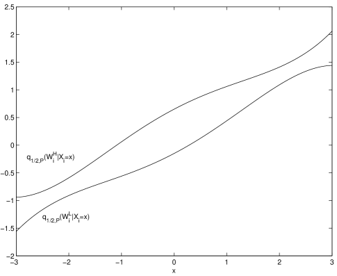
Figure 1: Conditional Medians of $W_{i}^{H}$ and $W_{i}^{L}$ for Quantile Regression Model

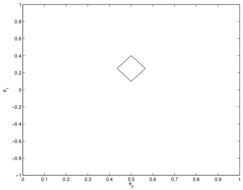
Figure 2: Identified Set for Quantile Regression Model

Figure 1 shows the true conditional medians $q_{1/2,P}(W_{i}^{H}|X_{i}=x)$ and $q_{1/2,P}(W_{i}^{L}|X_{i}=x)$ as a function of $x$ for this example. The true identified set $\Theta_{0}(P)$ for this example is the set of parameter values $(\theta_{1},\theta_{2})$ such that the line $\theta_{1}+\theta_{2}x$ is between these two conditional medians for every value of $x$ on the support of $X_{i}$. Figure 2 plots the boundary of this identified set. The identified set consists of all points outlined by the shape in this figure.

To illustrate the implementation of the set estimates in this paper applied to this model, I present a contour plot of the KS statistic evaluated at different values of the parameters for a single data set drawn from this data generating process. For a given choice of the critical value $\hat{c}_{n}$, the set estimate $\mathcal{C}_{n}(\hat{c}_{n})$ is then given by the set of points $(\theta_{1},\theta_{2})$ such that the KS statistic $T_{n}(\theta)$ given in this plot is less than or equal to $\hat{c}_{n}\sqrt{(\log n)/n}$. In other words, each of the level sets in this plot gives the boundary of $\mathcal{C}_{n}(\hat{c}_{n})$ for some choice of $\hat{c}_{n}$, with the level sets for larger values of the KS statistic corresponding to larger (more conservative) choices of $\hat{c}_{n}$.

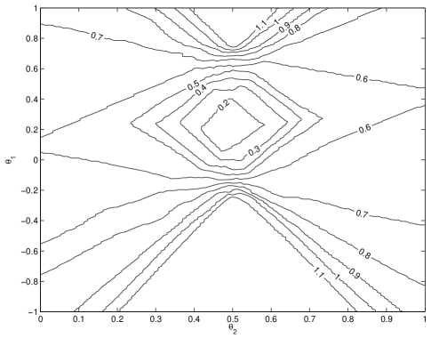
Figure 3: Contours of KS Statistic for Quantile Regression Model

The contour plot is shown in Figure 3. This plot was formed from a single data set of $n=500$ observations drawn from the data generating process described above. For the set of functions $\mathcal{G}$, I used the set of indicator functions for intervals $I(s<X<t)$. For the truncation point $\sigma_{n}$ for the standard deviation weights, I multiply $1/2$, the standard deviation of a single $\text{Bernoulli}(1/2)$ variable, by $\sqrt{(\log n)(\log\log n)/n}$, a sequence that converges to zero more slowly than $\sqrt{\log n/n}$ as required. I set $S(t_{1},t_{2})=\max(t_{1},t_{2},0)$.

For the monte carlo, I use the same choices of $\mathcal{G}$, $\sigma_{n}$, and $S$. For the critical value $\hat{c}_{n}$, I use the slowly increasing sequence $2\sqrt{\log\log n}$. Setting the critical value to $2$ regardless of $n$ leads to a somewhat conservative critical value for the case where $\mathcal{G}$ contains a single function. As $n$ increases, functions $I(s<X_{i}<t)$ with $s$ close to $t$ are given increasing weight, so that the KS statistic behaves like the maximum of an increasing number of standard normal variables, and the critical value increases appropriately (or slightly faster than needed). I generate monte carlo data sets with the data generating process described above and $n$ equal to $200$, $500$, and $1000$ observations. I use 1000 replications for each monte carlo design.

	quantiles
$n$	.25	.5	.75	.9	.95	coverage
200	0.45	0.5	0.54	0.59	0.62	100%
500	0.34	0.36	0.39	0.41	0.43	100%
1000	0.27	0.28	0.3	0.32	0.33	100%

Table 1: Summary Statistics for Hausdorff Distances for Monte Carlo

		quantiles
	$n$	.25	.5	.75	.9	.95
	200	0.45	0.49	0.53	0.57	0.59
$\theta_{1}$	500	0.34	0.36	0.38	0.41	0.43
	1000	0.26	0.28	0.3	0.32	0.33
	200	0.33	0.36	0.41	0.48	0.52
$\theta_{2}$	500	0.24	0.25	0.27	0.28	0.29
	1000	0.19	0.2	0.21	0.22	0.22

Table 2: Summary Statistics for Hausdorff Distances for Individual Parameters for Monte Carlo

		quantiles of $\hat{\ell}_{\theta_{i}}$					quantiles of $\hat{u}_{\theta_{i}}$
	$n$	.05	.1	.25	.5	.75	.25	.5	.75	.9	.95
	200	-0.47	-0.45	-0.4	-0.35	-0.31	0.81	0.86	0.9	0.95	0.98
$\theta_{1}$	500	-0.31	-0.3	-0.26	-0.23	-0.2	0.71	0.74	0.77	0.79	0.81
	1000	-0.22	-0.2	-0.18	-0.16	-0.14	0.64	0.67	0.69	0.71	0.72
	200	-0.05	0	0.05	0.1	0.14	0.87	0.9	0.95	1.01	1.06
$\theta_{2}$	500	0.16	0.17	0.18	0.2	0.22	0.78	0.8	0.82	0.83	0.84
	1000	0.22	0.23	0.24	0.25	0.27	0.73	0.75	0.76	0.77	0.78

Table 3: Summary Statistics for Set Estimates for Individual Parameters for Monte Carlo

Results are reported in Tables 1, 2 and 3. In Table 1, I report, for each sample size, the coverage probability (the proportion of the monte carlo replications for which the estimate contains the identified set) and quantiles of the Hausdorff distance between the estimate and the identified set. Even for the smallest sample size of $n=200$, the set estimate contains the identified set for every monte carlo replication. For the data generating process used in these monte carlos, Theorem 4.3 holds with $\alpha=2$, giving a rate of convergence of $((\hat{c}_{n}^{2}\log n)/n)^{\alpha/(d_{X}+2\alpha)}=((\hat{c}_{n}^{2}\log n)/n)^{2/5}$ (this follows from Theorem 5.4, since the upper and lower conditional medians are bounded away from each other and have smooth second derivatives, and regression lines corresponding to parameters on the boundary of the identified set are tangent to one of the conditional medians on the interior of the support of $X_{i}$). According to this result, the distance of the set estimate to the identified set should decrease by a factor of $.77$ going from $n=200$ to $n=500$, and should decrease again by a factor of $.81$ going from $n=500$ to $n=1000$. These asymptotic results give a decent approximation of the monte carlo results reported in Table 1, although the Hausdorff distances in this table decrease slightly more quickly.

The Hausdorff distance to the identified set summarizes the accuracy of the set estimator, but can be difficult to interpret, since it combines the accuracy of the estimate across both coordinates. Tables 2 and 3 report monte carlo results for the projections of the set estimate $\mathcal{C}_{n}(\hat{c}_{n})$ onto each coordinate. Define $\Theta_{1,\text{proj}}(P)=\{\theta|(\theta,\theta_{2})\in\Theta_{0}(P)\text{ some $\theta_{2}$}\}$ and $\Theta_{2,\text{proj}}(P)=\{\theta|(\theta_{1},\theta)\in\Theta_{0}(P)\text{ some $\theta_{1}$}\}$ to be the projections of the identified set onto each coordinate and $\mathcal{C}_{n,1,\text{proj}}(\hat{c}_{n})=\{\theta|(\theta,\theta_{2})\in\mathcal{C}_{n}(\hat{c}_{n})\text{ some $\theta_{2}$}\}$ and $\mathcal{C}_{n,2,\text{proj}}(\hat{c}_{n})=\{\theta|(\theta_{1},\theta)\in\mathcal{C}_{n}(\hat{c}_{n})\text{ some $\theta_{1}$}\}$ to be the corresponding projections of the set estimate. Let $[\hat{\ell}_{\theta_{i}},\hat{u}_{\theta_{i}}]$ be the smallest interval containing $\mathcal{C}_{n,i,\text{proj}}(\hat{c}_{n})$ for $i=1,2$. In Table 2, I report quantiles of the realizations of $d_{H}(\mathcal{C}_{n,1,\text{proj}}(\hat{c}_{n}),\Theta_{1,\text{proj}}(P))$ and $d_{H}(\mathcal{C}_{n,2,\text{proj}}(\hat{c}_{n}),\Theta_{2,\text{proj}}(P))$ for the monte carlo replications. In Table 3, I report quantiles of $\hat{\ell}_{\theta_{i}}$ and $\hat{u}_{\theta_{i}}$.

Table 2 reveals that the set estimate for the slope parameter $\theta_{2}$ has less sampling error in this case than the intercept parameter $\theta_{1}$. Indeed, the Hausdorff distances in Table 1 appear to be driven mostly by the intercept parameter. While estimation error in $\theta_{2}$ is generally smaller, than estimation error for the intercept parameter, the estimate for $\theta_{2}$ appears to be shrinking towards the identified set for $\theta_{2}$ at a similar rate.

Table 3 summarizes the finite sample behavior of the confidence intervals $[\hat{\ell}_{\theta_{i}},\hat{u}_{\theta_{i}}]$ for each $\theta_{i}$ generated from the set estimate $\mathcal{C}_{n}(\hat{c}_{n})$. While these confidence intervals for individual coordinates contain less information than the confidence region $\mathcal{C}_{n}(\hat{c}_{n})$ for the identified set, they are less cumbersome to report and summarize. For comparison, the projection of the true identified set onto the intercept coordinate $\theta_{2}$ is $\Theta_{1,\text{proj}}(P)=[.17,.33]$, and the projection of the true identified set onto the slope coordinate $\theta_{2}$ is $\Theta_{2,\text{proj}}(P)=[.47,.53]$. Note that the confidence interval for the slope parameter $\theta_{2}$ contains only positive values for 90% of the monte carlo replications even with the smallest sample size of 200 observations. Thus, one would correctly conclude that $\theta_{2}$ is positive for an overwhelming proportion of realizations of the data even with a relatively small sample size, despite the conservative nature of the estimate $\mathcal{C}_{n}(\hat{c}_{n})$.

8 Conclusion

This paper proposes estimates of the identified set in conditional moment inequality models based on variance weighted KS statistics. I derive rates of convergence of these and other set estimators to the identified set under conditions that apply to many models of practical interest. In many settings, the rate of convergence of the set estimator I propose is the fastest among those available, and, in settings where other estimators are better, the improvement in rate of convergence is no more than a factor of $\log n$. While, in most cases, there is some other estimator that does slightly better, choosing the correct one requires knowledge of smoothness and shape conditions on the data generating process, and guessing incorrectly about these conditions can lead the researcher to use an estimator with a much slower rate of convergence. The advantage of the estimator proposed in this paper is that it performs well under a variety of conditions without prior knowledge of which of these conditions hold.

In settings where local alternatives violate the conditional moment inequalities on a shrinking set, the weights I propose for KS statistics give the statistics more power against local alternatives than bounded weights. The examples in Section 5 show that this situation is common in practice. When sequences of local alternatives violate the conditional moment inequalities on a fixed, positive probability set, the larger critical values required by the increasing sequence of weight functions lead to a loss in power, but only by a factor of $(\log n)^{1/2}$. This provides a theoretical justification for variance weighting in this context. Under certain conditions, weighting the KS statistic objective function by a truncated inverse of the estimated variance increases the rate of convergence of the corresponding estimator of the identified set.

Appendix A Appendix

This appendix collects several results not stated in the body of the paper. In Section A.1, I state and prove uniform convergence results for classes of functions weighted by truncated standard deviations. These results are used later in the appendix in proving some of the results stated in the body of the paper. In Section A.2, I provide sufficient conditions for the rate of convergence to be strictly faster than $\sqrt{n}$. In Section A.3, I provide an example of a data generating process for an interval regression where low power against local alternatives when the slope parameter varies leads to a slower rate of convergence to the identified set. In Section A.4, I state conditions under which Assumption 3.2 holds and verify them for the applications described in Section 5. Section A.5 contains proofs of the theorems stated in the body of the paper.

A.1 Uniform Convergence Lemma

The following lemma is useful in deriving some of these results. Applied to mean zero functions, the lemma says that any sequence of classes of functions that is not too complex converges uniformly at a $\sqrt{n/\log n}$ rate when scaled by the standard deviation if the minimum standard deviation does not go to zero too fast.

Lemma A.1.

Let $Z_{1},\ldots,Z_{n}$ be iid observations and let $\mathcal{P}$ be a set of probability distributions and $\mathcal{F}_{n,P}$ a set of classes of functions indexed by $n\in\mathbb{N}$ and $P\in\mathcal{P}$ such that, for some $\overline{f}$, $f(Z_{i})\leq\overline{f}$ with $P$-probability one for $P\in\mathcal{P}$ and $f\in\mathcal{F}_{n,P}$ for each $n$. Let $\mu_{2,P}(f)=(E_{P}f(Z_{i})^{2})^{1/2}$ and let $\mu_{2,n}$ be a sequence such that $\mu_{2,n}\sqrt{n/\log n}$ is bounded away from zero. Let $\mathcal{G}_{n,P}=\{f\mu_{2,n}/(\mu_{2,P}(f)\vee\mu_{2,n})|f\in\mathcal{F}_{n,P}\}$ and suppose that

$$\sup_{P\in\mathcal{P}}\,\sup_{n\in\mathbb{N}}\,\sup_{Q}N(\varepsilon,\mathcal{G}_{n,P},L_{1}(Q))\leq A\varepsilon^{-W}$$

for $0<\varepsilon<1$ where the supremum over $Q$ is over all probability measures. Then for some $B$ that does not depend on $N$,

$$\sup_{P\in\mathcal{P}}P\left(\frac{\sqrt{n}}{\sqrt{\log n}}\sup_{f\in\mathcal{F}_{n,P}}\left|(E_{n}-E_{P})\frac{f(Z_{i})}{\mu_{2,P}(f)\vee\mu_{2,n}}\right|\geq B\,\text{some $n\geq N$}\right)\stackrel{{\scriptstyle N\to\infty}}{{\to}}0.$$

Proof.

The result follows by applying the following theorem to the classes of functions $\mathcal{G}_{n,P}$. For $g=f\mu_{2,n}/(\mu_{2,P}(f)\vee\mu_{2,n})\in\mathcal{G}_{n,P}$, $E_{P}g(Z_{i})^{2}=E_{P}f(Z_{i})^{2}\mu_{2,n}^{2}/(\mu_{2,P}(f)^{2}\vee\mu_{2,n}^{2})=\mu_{2,P}(f)^{2}\mu_{2,n}^{2}/(\mu_{2,P}(f)^{2}\vee\mu_{2,n}^{2})\leq\mu_{2,n}^{2}$, so the theorem applies with the same $\mu_{2,n}$. ∎

Specialized to a class $\mathcal{P}$ of probability distributions with a single element $P$, this says that the sequence in the probability statement in the last display of the lemma is bounded by $B$ with $P$-probability one. The conclusion of the lemma implies that this scaled sequence is $\mathcal{O}_{P}(1)$ uniformly in $P\in\mathcal{P}$, but is slightly stronger.

The proof of the lemma uses the following theorem, which is a slightly stronger version of Theorem 37 in Pollard (1984), with the conditions stated in a slightly different way. The following theorem basically follows the arguments of the proof of Theorem 37 in Pollard (1984), but changes a few things to get a slightly stronger result. Note that the notation $\mu_{2,P}^{2}$ is used for the raw second moment of functions rather than their variance, although the distinction is often not important since applications typically involve the raw second moment going to zero at the same rate as the variance.

Theorem A.1.

Let $Z_{1},\ldots,Z_{n}$ be iid observations and let $\mathcal{P}$ be a set of probability measures and $\mathcal{F}_{n,P}$ a set of classes of functions indexed by $n\in\mathbb{N}$ and $P\in\mathcal{P}$ such that, for some $\overline{f}$, $f(Z_{i})\leq\overline{f}$ $P$-a.s. for $f\in\mathcal{F}_{n,P}$ for $P\in\mathcal{P}$ for each $n$ and, for some positive constants $A$ and $W$,

$$\sup_{P\in\mathcal{P}}\,\sup_{n\in\mathbb{N}}\,\sup_{Q}N(\varepsilon,\mathcal{F}_{n,P},L_{1}(Q))\leq A\varepsilon^{-W}$$

for $0<\varepsilon<1$ where the supremum over $Q$ is over all probability measures. Suppose that, for some sequence $\mu_{2,n}$, $E_{P}f(Z_{i})^{2}\leq\mu_{2,n}^{2}$ for all $f\in\mathcal{F}_{n,P}$ for all $P\in\mathcal{P}$ for all $n$. Then, if $\mu_{2,n}\sqrt{n/\log n}$ is bounded away from zero we will have, for some $B$ that does not depend on $N$,

$$\sup_{P\in\mathcal{P}}P\left(\frac{\sqrt{n}}{\mu_{2,n}\sqrt{\log n}}\sup_{f\in\mathcal{F}_{n,P}}\left|(E_{n}-E_{P})f(Z_{i})\right|\geq B\,\text{some $n\geq N$}\right)\stackrel{{\scriptstyle N\to\infty}}{{\to}}0.$$

Proof.

The proof is a slight modification of the proof of Theorem 37 in Pollard (1984). The sequence $\mu_{2,n}$ corresponds to $\delta_{n}$ in that theorem, and, in contrast to the theorem from Pollard (1984) which defines a sequence $\alpha_{n}$ that must satisfy certain conditions, this theorem corresponds to using the best $\alpha_{n}$ sequence possible, and noting that $\alpha_{n}$ need not be nonincreasing as long as it is bounded.

Without loss of of generality, assume that $\overline{f}=1$. Fix $B$ (conditions on how large $B$ has to be will be stated throughout the theorem) and set $\varepsilon_{n}=\frac{B\mu_{2,n}\sqrt{\log n}}{8\sqrt{n}}$. Since $var_{P}((E_{n}-E_{P})f(Z_{i}))/(4\varepsilon_{n}^{2})\leq(\mu_{2,n}^{2}/n)/(4B^{2}\mu_{2,n}^{2}(\log n)/(64n))=16/(B^{2}\log n)\leq 1/2$ for $n$ greater than some number that does not depend on $P$, the inequality (30) in Pollard (1984) will eventually imply

$$P\left(\frac{\sqrt{n}}{\mu_{2,n}\sqrt{\log n}}\sup_{f\in\mathcal{F}_{n,P}}\left|(E_{n}-E)f(Z_{i})\right|\geq B\right)=P\left(\sup_{f\in\mathcal{F}_{n,P}}\left|(E_{n}-E)f(Z_{i})\right|\geq 8\varepsilon_{n}\right)$$

$$\leq 4(P\times\nu)\left(\sup_{f\in\mathcal{F}_{n,P}}\left|\mathbb{P}_{n}^{\circ}f(Z_{i})\right|\geq 2\varepsilon_{n}\right)$$

for all $P\in\mathcal{P}$ where $\mathbb{P}_{n}^{\circ}f(Z_{i})=\frac{1}{n}\sum_{i=1}^{n}f(Z_{i})\cdot s_{i}$ and $s_{1},\ldots,s_{n}$ are iid random variables that take on values $\pm 1$ each with probability one half drawn independent of $Z_{1},\ldots,Z_{n}$ and $\nu$ denotes the probability measure of $s_{1},\ldots,s_{n}$. Conditional on the data, this is bounded by

$$(P\times\nu)\left(\sup_{f\in\mathcal{F}_{n}}\left|\mathbb{P}_{n}^{\circ}f(Z_{i})\right|\geq 2\varepsilon_{n}\bigg{|}Z_{1},\ldots,Z_{n}\right)\leq 2N(\varepsilon_{n},\mathcal{F}_{n,P},L_{1}(\mathbb{P}_{n}))\exp\left[-\frac{1}{2}\frac{n\varepsilon_{n}^{2}}{\left(\sup_{f\in\mathcal{F}_{n,P}}E_{n}f(Z_{i})^{2}\right)}\right].$$

For any constant $a>0$, on the event that

$$\sup_{f\in\mathcal{F}_{n,P}}E_{n}f(Z_{i})^{2}\leq a^{2}\mu_{2,n}^{2},$$ (5)

the previous display will be bounded by

$$2N(\varepsilon_{n},\mathcal{F}_{n,P},L_{1}(\mathbb{P}_{n}))\exp\left(-\frac{1}{2}\frac{n\varepsilon_{n}^{2}}{a^{2}\mu_{2,n}^{2}}\right)\leq 2A\varepsilon_{n}^{-W}\exp\left(-\frac{1}{2}\frac{n\varepsilon_{n}^{2}}{a^{2}\mu_{2,n}^{2}}\right)$$

$$=2A\exp\left[-\frac{1}{2}\cdot n\cdot\frac{B^{2}\mu_{2,n}^{2}\log n}{64n}\cdot\frac{1}{a^{2}\mu_{2,n}^{2}}-W\log\frac{B\mu_{2,n}\sqrt{\log n}}{8\sqrt{n}}\right]$$

$$=2A\exp\left[-\frac{B^{2}\log n}{128a^{2}}-W\log\frac{B}{8}-W\log\frac{\mu_{2,n}\sqrt{\log n}}{\sqrt{n}}\right]$$

The condition that $\mu_{2,n}\sqrt{n/\log n}$ is bounded away from zero is more than enough to guarantee that the term in the last logarithm is bounded from below by a fixed power of $n$. Thus, the expression in the last display can be made to go to zero at any polynomial rate for any $a$ by choosing $B$ to be large enough (in a way that depends on $a$ but not $n$ or $P$).

For any $P\in\mathcal{P}$, the $P$-probability of (5) failing to hold can be bounded using Lemma 33 in Pollard (1984) with $\delta_{n}=a\mu_{2,n}/8$ (the lemma holds for $a\geq 8$):

$$P\left(\sup_{f\in\mathcal{F}_{n,P}}E_{n}f(Z_{i})^{2}>a^{2}\mu_{2,n}^{2}\right)=P\left(\sup_{f\in\mathcal{F}_{n,P}}E_{n}f(Z_{i})^{2}>64\delta_{n}^{2}\right)\leq 4E_{P}[N(\delta_{n},\mathcal{F}_{n,P},L_{2}(\mathbb{P}_{n}))]\exp(-n\delta_{n}^{2})$$

$$\leq 4A(\delta_{n}/2)^{-W}\exp(-n\delta_{n}^{2})=4\cdot 2^{W}A\exp(-n\delta_{n}^{2}-W\log\delta_{n})$$

$$=4\cdot 2^{W}A\exp\left[-na^{2}\mu_{2,n}^{2}/64-W\log\frac{a}{8}-W\log\mu_{2,n}\right]$$

$$\leq 4\cdot 2^{W}A\exp\left[-\frac{na^{2}}{64}\frac{c\log n}{n}-W\log\frac{a}{8}-\frac{W}{2}\log\frac{c\log n}{n}\right]$$

where $\sqrt{c}$ is a lower bound for $\mu_{2,n}\sqrt{n/\log n}$. This can be made to go to zero at any polynomial rate by choosing $a$ large.

Thus, if we choose $a$ and $B$ large enough, $\sup_{P\in\mathcal{P}}P\left(\frac{\sqrt{n}}{\mu_{2,n}\sqrt{\log n}}\sup_{f\in\mathcal{F}_{n,P}}\left|(E_{n}-E_{P})f(Z_{i})\right|\geq B\right)$ will be summable over $n$, so that

$$\sup_{P\in\mathcal{P}}P\left(\frac{\sqrt{n}}{\mu_{2,n}\sqrt{\log n}}\sup_{f\in\mathcal{F}_{n,P}}\left|(E_{n}-E_{P})f(Z_{i})\right|\geq B\,\text{some $n\geq N$}\right)$$

$$\leq\sum_{n\geq N}\sup_{P\in\mathcal{P}}P\left(\frac{\sqrt{n}}{\mu_{2,n}\sqrt{\log n}}\sup_{f\in\mathcal{F}_{n,P}}\left|(E_{n}-E_{P})f(Z_{i})\right|\geq B\right)\stackrel{{\scriptstyle N\to\infty}}{{\to}}0.$$

∎

With this lemma in hand, we can get rates of convergence for classes of functions weighted by their standard deviation under additional conditions that allow the standard deviation to be consistently estimated. In order to get results for functions weighted by the standard deviation rather than the raw second moment, I apply the previous results to classes of functions of the form $f-E_{P}f(Z_{i})$. Letting $\hat{\sigma}(f)^{2}=E_{n}(f(Z_{i}))^{2}-(E_{n}f(Z_{i}))^{2}$ and $\sigma_{P}(f)^{2}=E_{P}(f(Z_{i}))^{2}-(E_{P}f(Z_{i}))^{2}$, rates of convergence for

$$\sup_{f\in\mathcal{F}_{n}}\left|(E_{n}-E_{P})\frac{f(Z_{i})}{\hat{\sigma}(f)\vee\sigma_{n}}\right|$$

will follow by applying the above results to the classes of functions $f-E_{P}f(Z_{i})$ once we can bound $\frac{\sigma_{P}(f)\vee\sigma_{n}}{\hat{\sigma}(f)\vee\sigma_{n}}$, and for this it is sufficient to show that $\hat{\sigma}(f)/\sigma_{P}(f)$ converges to one uniformly over $\sigma_{P}(f)\geq\sigma_{n}$. The following lemma gives sufficient conditions for this.

Lemma A.2.

Let $Z_{1},\ldots,Z_{n}$ be iid observations and let $\mathcal{F}_{n}$ be a sequence of classes of functions and $\mathcal{P}$ a set of probability distributions such that, for some $\overline{f}$, $f(Z_{i})\leq\overline{f}$ with $P$-probability one for $P\in\mathcal{P}$ and $f\in\mathcal{F}_{n}$ for each $n$. Let $\sigma_{P}(f)=(E_{P}f(Z_{i})^{2}-(E_{P}f(Z_{i}))^{2})^{1/2}$ and let $\sigma_{n}$ be a sequence such that $\sigma_{n}\sqrt{n/\log n}$ is bounded away from zero. Define $\mathcal{G}_{n,P}^{1}=\{(f-E_{P}f(Z_{i}))\sigma_{n}/(\sigma_{P}(f)\vee\sigma_{n})\}$ and $\mathcal{G}_{n,P}^{2}=\{(f-E_{P}f(Z_{i}))^{2}\sigma_{n}/(\mu_{2,P}([f-E_{P}f(Z_{i})]^{2})\vee\sigma_{n})\}$, and suppose that, for some positive constants $A$ and $W$,

$$\sup_{P\in\mathcal{P}}\,\sup_{n\in\mathbb{N}}\,\sup_{Q}N(\varepsilon,\mathcal{G}_{n,P}^{i},L_{1}(Q))\leq A\varepsilon^{-W}$$

for $0<\varepsilon<1$ and $i=1,2$, where the supremum over $Q$ is over all probability measures.

Then, for every $\varepsilon>0$, there exists a $c$ such that, if $\sigma_{n}\sqrt{n/\log n}\geq c$ for all $n$,

$$\sup_{P\in\mathcal{P}}P\left(\sup_{f\in\mathcal{F}_{n},\sigma_{P}(f)\geq\sigma_{n}}\left|\frac{\hat{\sigma}(f)}{\sigma_{P}(f)}-1\right|\geq\varepsilon\,\text{some $n\geq N$}\right)\stackrel{{\scriptstyle N\to\infty}}{{\to}}0.$$

Proof.

We have

$$\sup_{f\in\mathcal{F}_{n},\sigma_{P}(f)\geq\sigma_{n}}\left|\frac{\hat{\sigma}^{2}(f)-\sigma_{P}^{2}(f)}{\sigma_{P}^{2}(f)}\right|$$

$$=\sup_{f\in\mathcal{F}_{n},\sigma_{P}(f)\geq\sigma_{n}}\left|\frac{(E_{n}-E_{P})(f(Z_{i})-E_{P}f(Z_{i}))^{2}-(E_{n}f(Z_{i})-E_{P}f(Z_{i}))^{2}}{\sigma_{P}^{2}(f)}\right|$$

$$\leq\sup_{f\in\mathcal{F}_{n},\sigma_{P}(f)\geq\sigma_{n}}\left|\frac{(E_{n}-E_{P})(f(Z_{i})-E_{P}f(Z_{i}))^{2}}{\sigma_{P}^{2}(f)}\right|+\left|\frac{[(E_{n}-E_{P})f(Z_{i})]^{2}}{\sigma_{P}^{2}(f)}\right|.$$ (6)

The first term is equal to

$$\left|\frac{(E_{n}-E_{P})(f(Z_{i})-E_{P}f(Z_{i}))^{2}}{\mu_{2,P}([f-E_{P}f(Z_{i})]^{2})\vee\sigma_{n}}\right|\frac{\mu_{2,P}([f-E_{P}f(Z_{i})]^{2})\vee\sigma_{n}}{\sigma_{P}^{2}(f)}.$$

We have $\mu_{2,P}([f-E_{P}f(Z_{i})]^{2})^{2}=E_{P}[f(Z_{i})-E_{P}f(Z_{i})]^{4}\leq 4\overline{f}^{2}E_{P}[f(Z_{i})-E_{P}f(Z_{i})]^{2}=4\overline{f}^{2}\sigma_{P}(f)^{2}$ so that

$$\frac{\mu_{2,P}([f-E_{P}f(Z_{i})]^{2})\vee\sigma_{n}}{\sigma_{P}^{2}(f)}\leq\frac{[2\overline{f}\sigma_{P}(f)]\vee\sigma_{n}}{\sigma_{P}^{2}(f)}\leq\frac{2\overline{f}\vee 1}{\sigma_{P}(f)}\leq\frac{2\overline{f}\vee 1}{\sigma_{n}}$$

where the last two inequalities hold for $\sigma_{P}(f)\geq\sigma_{n}$. Thus, for any $\varepsilon>0$,

$$\sup_{P\in\mathcal{P}}P\left(\sup_{f\in\mathcal{F}_{n},\sigma_{P}(f)\geq\sigma_{n}}\left|\frac{(E_{n}-E_{P})(f(Z_{i})-E_{P}f(Z_{i}))^{2}}{\sigma_{P}^{2}(f)}\right|\geq\varepsilon\,\text{some $n\geq N$}\right)$$

$$\leq\sup_{P\in\mathcal{P}}P\left(\sup_{f\in\mathcal{F}_{n},\sigma_{P}(f)\geq\sigma_{n}}\frac{2\overline{f}\vee 1}{\sigma_{n}}\left|\frac{(E_{n}-E_{P})(f(Z_{i})-E_{P}f(Z_{i}))^{2}}{\left\{E[(f(Z_{i})-E_{P}f(Z_{i}))^{2}]^{2}\right\}^{(1/2)}\vee\sigma_{n}}\right|\geq\varepsilon\,\text{some $n\geq N$}\right)$$

$$\leq\sup_{P\in\mathcal{P}}P\left(\sup_{f\in\mathcal{F}_{n},\sigma_{P}(f)\geq\sigma_{n}}\frac{\sqrt{n}}{\sqrt{\log n}}\left|\frac{(E_{n}-E_{P})(f(Z_{i})-E_{P}f(Z_{i}))^{2}}{\left\{E[(f(Z_{i})-E_{P}f(Z_{i}))^{2}]^{2}\right\}^{(1/2)}\vee\sigma_{n}}\right|\geq c\varepsilon/(2\overline{f}\vee 1)\,\text{some $n\geq N$}\right)$$

where the last inequality holds for $\sigma_{n}\sqrt{n/\log n}\geq c$. By Lemma A.1, this will go to zero if $c$ is large enough so that $c\varepsilon/(2\overline{f}\vee 1)$ is greater than the $B$ for which the conclusion of Lemma A.1 holds for the class $\mathcal{G}_{n,P}^{2}$.

The probability that the second term in the last line of Equation A.1 is greater than $\varepsilon>0$ for some $n\geq N$ goes to zero uniformly in $P\in\mathcal{P}$ by Lemma A.1 with the class $\{f-E_{P}f(Z_{i})|f\in\mathcal{F}_{n}\}$ taking the place of $\mathcal{F}_{n,P}$ in that lemma. ∎

Combining these lemmas gives a consistency result for classes of functions weighted by their standard deviations. The conditions are the same as those for Lemma A.2.

Lemma A.3.

Let $Z_{1},\ldots,Z_{n}$ be iid observations and let $\mathcal{F}_{n}$ be a sequence of classes of functions and $\mathcal{P}$ a set of probability distributions such that, for some $\overline{f}$, $f(Z_{i})\leq\overline{f}$ with $P$-probability one for $P\in\mathcal{P}$ and $f\in\mathcal{F}_{n}$ for each $n$. Let $\sigma_{P}(f)=(E_{P}f(Z_{i})^{2}-(E_{P}f(Z_{i}))^{2})^{1/2}$. Define $\mathcal{G}_{n,P}^{1}=\{(f-E_{P}f(Z_{i}))\sigma_{n}/(\sigma_{P}(f)\vee\sigma_{n})\}$ and $\mathcal{G}_{n,P}^{2}=\{(f-E_{P}f(Z_{i}))^{2}\sigma_{n}/(\mu_{2,P}([f-E_{P}f(Z_{i})]^{2})\vee\sigma_{n})\}$, and suppose that, for some positive constants $A$ and $W$,

$$\sup_{P\in\mathcal{P}}\,\sup_{n\in\mathbb{N}}\,\sup_{Q}N(\varepsilon,\mathcal{G}_{n,P}^{i},L_{1}(Q))\leq A\varepsilon^{-W}$$

for $0<\varepsilon<1$ and $i=1,2$, where the supremum over $Q$ is over all probability measures.

Then, for some $B$ and $c$ that do not depend on $N$ or $P$, if $\sigma_{n}\sqrt{n/\log n}\geq c$ for all $n$,

$$\sup_{P\in\mathcal{P}}P\left(\sup_{f\in\mathcal{F}_{n}}\frac{\sqrt{n}}{\sqrt{\log n}}\left|\frac{f(Z_{i})-E_{P}(f(Z_{i}))}{\hat{\sigma}(f)\vee\sigma_{n}}\right|\geq B\,\text{some $n\geq N$}\right)\stackrel{{\scriptstyle N\to\infty}}{{\to}}0.$$

Proof.

We have

$$P\left(\sup_{f\in\mathcal{F}_{n}}\frac{\sqrt{n}}{\sqrt{\log n}}\left|\frac{f(Z_{i})-E_{P}(f(Z_{i}))}{\hat{\sigma}(f)\vee\sigma_{n}}\right|\geq B\,\text{some $n\geq N$}\right)$$

$$=P\left(\sup_{f\in\mathcal{F}_{n}}\frac{\sqrt{n}}{\sqrt{\log n}}\left|\frac{f(Z_{i})-E_{P}(f(Z_{i}))}{\sigma_{P}(f)\vee\sigma_{n}}\right|\frac{\sigma_{P}(f)\vee\sigma_{n}}{\hat{\sigma}(f)\vee\sigma_{n}}\geq B\,\text{some $n\geq N$}\right)$$

$$\leq P\left(\sup_{f\in\mathcal{F}_{n}}\frac{\sqrt{n}}{\sqrt{\log n}}\left|\frac{f(Z_{i})-E_{P}(f(Z_{i}))}{\sigma_{P}(f)\vee\sigma_{n}}\right|\geq B/2\,\text{some $n\geq N$}\right)$$

$$+P\left(\inf_{f\in\mathcal{F}_{n}}\frac{\hat{\sigma}(f)\vee\sigma_{n}}{\sigma_{P}(f)\vee\sigma_{n}}\leq 1/2\,\text{some $n\geq N$}\right).$$

The second to last line goes to zero uniformly in $P\in\mathcal{P}$ by Lemma A.1 applied to the classes $\{f-E_{P}(f)|f\in\mathcal{F}_{n},P\in\mathcal{P}\}$ (here, $B$ must be chosen large enough so that the conclusion of this lemma holds with $B$ replaced by $B/2$). Since $\frac{\hat{\sigma}(f)\vee\sigma_{n}}{\sigma_{P}(f)\vee\sigma_{n}}\geq 1>1/2$ when $\sigma_{P}(f)<\sigma_{n}$, the last line is bounded by

$$P\left(\inf_{f\in\mathcal{F}_{n},\sigma_{P}(f)\geq\sigma_{n}}\frac{\hat{\sigma}(f)}{\sigma_{P}(f)}\leq 1/2\,\text{some $n\geq N$}\right),$$

which goes to zero uniformly in $P\in\mathcal{P}$ if $\sigma_{n}\sqrt{n/\log n}\geq c$ for $c$ large enough by Lemma A.2.

∎

A.2 Conditions for Exact Rate of Convergence

If $\sigma_{n}$ is fixed, we will have a $\sqrt{n}$ rate of uniform convergence for the KS statistic. The $\sqrt{n/\log n}$ rate of convergence results used in Theorem 3.1 do not rule this out for the case where $\sigma_{n}$ goes to zero, but another argument shows that the rate of convergence will be strictly slower than $\sqrt{n}$ in many situations.

Assumption A.1.

For some $\theta\in\Theta_{0}(P)$, some $j$, and some open set $\mathcal{X}$, the following hold. (i) $E_{P}(m_{j}(W_{i},\theta)|X_{i})=0$ a.s. on $\mathcal{X}$ and $X_{i}$ has a density $f_{X}(x)$ on $\mathcal{X}$ that is bounded from above and from below away from zero. (ii) $var(m(W_{i},\theta)|X_{i}=x)$ is continuous as a function of $x$ and bounded away from zero and infinity on $\mathcal{X}$. (iii) $\mathcal{G}$ contains the function $t\mapsto k((t-x)/h)$ for all $x$ and all $h$ less than some fixed positive constant where $k$ satisfies Assumption 6.2 and is continuous at zero.

The assumption on the set of functions $\mathcal{G}$ covers many commonly used cases, including indicator sets for $d_{X}$ dimensional rectangles or boxes.

Theorem A.2.

If Assumption A.1 holds and $S$ satisfies Assumption 3.4, then, if $\sigma_{n}\to 0$, $\sqrt{n}T_{n}(\theta)$ will diverge to $\infty$.

Proof.

Fix any points $x_{1},\ldots,x_{\ell}\in\mathcal{X}$. For $k$ from $1$ to $\ell$, let $g_{n,k}(t)=k((t-x_{k})/h_{n})$

$$Z_{n,k}=\frac{1}{\hat{\sigma}_{n,j}(\theta,g_{n,k})\vee\sigma_{n}}E_{n}m_{j}(W_{i},\theta)k((X_{i}-x_{k})/h_{n})$$

where $h_{n}$ is a sequence going to zero such that $h_{n}^{d_{X}/2}/\sigma_{n}$ goes to infinity and $h_{n}^{d_{X}/2}\geq n^{-\alpha}$ for some $\alpha<1$. By the assumption on $S$, $\sqrt{n}T_{n}(\theta)$ will diverge to $\infty$ if $\inf_{x,h,j}\frac{1}{\hat{\sigma}_{n,j}(\theta,x,h)\vee\sigma_{n}}E_{n}m_{j}(W_{i},\theta)k((X_{i}-x)/h)$ diverges to $-\infty$, and, for this, it is sufficient to show that $\min_{k}Z_{n,k}$ can be made arbitrarily small asymptotically by making $\ell$ large enough. Using standard arguments, it can be shown that $\hat{\sigma}_{n,j}(\theta,g_{n,k})/\sigma_{P,j}(\theta,g_{n,k})$ converges in probability to one, and, since $\sigma_{P,j}(\theta,g_{n,k})/h_{n}^{d/2}$ converges to a constant under these assumptions, we also have that

$$Z_{n,k}=\frac{1}{\hat{\sigma}_{n,j}(\theta,g_{n,k})}E_{n}m_{j}(W_{i},\theta)k((X_{i}-x_{k})/h_{n})$$

with probability approaching one. By the Lindeberg central limit theorem, defining

$$\tilde{Z}_{n,k}\equiv\frac{1}{\sigma_{P,j}(\theta,g_{n,k})}E_{n}m_{j}(W_{i},\theta)k((X_{i}-x_{k})/h_{n})$$

$(\sqrt{n}\tilde{Z}_{n,1},\ldots,\sqrt{n}\tilde{Z}_{n,\ell})$ converges to a vector of independent standard normal variables, so, since each $Z_{n,k}$ is eventually equal to $\tilde{Z}_{n,k}$ times something that converges to one, $(\sqrt{n}Z_{n,1},\ldots,\sqrt{n}Z_{n,\ell})$ also converges to a vector of independent standard normal variables. Thus, $\min_{k}\sqrt{n}Z_{n,k}$ converges to the minimum of $\ell$ independent standard normal variables, which can be made arbitrarily small by making $\ell$ large.

∎

A.3 Rates of Convergence for Slope Parameters

In this section of the appendix, I present a counterexample that shows that a condition along the lines of part (iii) of Assumption 5.4 is necessary to obtain the rate of convergence in Theorem 5.2. As discussed below, a similar counterexample shows that a condition on the parameter space $\Theta$ such as Assumption 5.3 is necessary in Theorem 5.1. These counterexamples also show that the first display in Assumption 4.4 cannot be replaced with an assumption that only takes into account the magnitude of the derivative vector. Consider an example where $E_{P}(W_{i}^{H}|X_{i}=x)=x^{2}$, $E_{P}(W_{i}^{L}|X_{i}=x)=-x^{2}$, $var(W_{i}^{H}|X_{i})=var(W_{i}^{L}|X_{i})=1$, and $X_{i}$ is has a uniform distribution on $[-1/2,1/2]$. Suppose that we use the set of functions $\{I(s<X_{i}<s+t)|s\in\mathbb{R},t\geq 0\}$.

In this case, the identified set is a single point $(0,0)$. Consider the sequence of local alternatives given by $\theta_{n}=(0,b_{n})$. We have, for all $s,t$ with $-1/2\leq s\leq s+t\leq 1/2$,

$$E_{P}[(W_{i}^{H}-b_{n}X_{i})I(s<X_{i}<s+t)]=E_{P}[(X_{i}^{2}-b_{n}X_{i})I(s<X_{i}<s+t)]$$

$$=\int_{s}^{s+t}(x^{2}-b_{n}x)\,dx=\int_{s}^{s+t}[(x-b_{n}/2)^{2}-b_{n}^{2}/4]\,dx$$

$$\geq\int_{-t/2}^{t/2}[u^{2}-b_{n}^{2}/4]\,du=2\left[\frac{1}{3}u^{3}-\frac{b_{n}^{2}}{4}u\right]_{u=0}^{t/2}=2t\left[\frac{1}{24}t^{2}-\frac{b_{n}^{2}}{8}\right]$$

and

$$var_{P}[(W_{i}^{H}-b_{n}X_{i})I(s<X_{i}<s+t)]\geq E_{P}\{var_{P}[(W_{i}^{H}-b_{n}X_{i})I(s<X_{i}<s+t)|X_{i}]\}$$

$$=E_{P}[I(s<X_{i}<s+t)]=t.$$

Thus, for $s,t$ such that $E_{P}[(W_{i}^{H}-b_{n}X_{i})I(s<X_{i}<s+t)]$ is negative,

$$\left|\frac{E_{P}[(W_{i}^{H}-b_{n}X_{i})I(s<X_{i}<s+t)]}{\{var_{P}[(W_{i}^{H}-b_{n}X_{i})I(s<X_{i}<s+t)]\}^{1/2}}\right|\leq 2t^{1/2}\left|\frac{1}{24}t^{2}-\frac{b_{n}^{2}}{8}\right|_{-}\leq\frac{3^{1/4}}{4}b_{n}^{1/2}b_{n}^{2}.$$

A symmetric argument applies to moments based on $W_{i}^{L}$. For some constant $K$, this sequence of local alternatives will be in $\mathcal{C}_{n}(\hat{c}_{n})$ if $b_{n}^{5/2}\leq K((\log n)/n)^{1/2}$ iff. $b_{n}\leq K((\log n)/n)^{1/5}$. In contrast, convergence to the identified set for one sided regression will be at a $((\log n)/n)^{2/5}$ rate if the parameter space $\Theta$ is restricted so that the absolute value of the slope parameter cannot be too large.

Now consider the one sided regression model of Section 5.1 with $E_{P}(W_{i}^{H}|X_{i}=x)=x^{2}$ and the parameter space $\Theta$ given by $[0,\infty)\times\mathbb{R}$. That is, the parameter space $\Theta$ incorporates the prior knowledge that the intercept is nonnegative. Again, the identified set is the point $(0,0)$, and the Hausdorff distance between the set estimate $\mathcal{C}_{n}(\hat{c}_{n})$ and the identified set will be at least $b_{n}$ if $\mathcal{C}_{n}(\hat{c}_{n})$ contains the point $(0,b_{n})$. By the same argument used above, $(0,b_{n})$ will be in $\mathcal{C}_{n}(\hat{c}_{n})$ for some sequence $b_{n}$ going to zero at a $((\log n)/n)^{1/5}$ rate, so that the rate of convergence of $\mathcal{C}_{n}(\hat{c}_{n})$ to the identified set will be no faster than $((\log n)/n)^{1/5}$, which is slower than the $((\log n)/n)^{2/5}$ rate given by Theorem 5.1 when the intercept is not restricted. Note that, in the case where the intercept parameter is not restricted a priori, the sequence of local alternatives $(0,b_{n})$ will still be in the estimate $\mathcal{C}_{n}(\hat{c}_{n})$, but the distance of these points to the identified set will no longer be equal to $b_{n}$, since the identified set will contain a point $(\theta^{\prime}(b_{n}),b_{n})$ for some $\theta^{\prime}(b_{n})$ that is smaller in magnitued than $b_{n}$.

A.4 Covering Number Conditions

In this section, I state some simple sufficient conditions under which Assumption 3.2 holds. I first prove that Assumption 3.2 holds under individual bounds on the complexity of the classes $\mathcal{G}$ and $\{w\mapsto m(w,\theta)|\theta\in\Theta\}$. The proof of this result uses Lemma A.4, stated and proved at the end of the section. I then provide examples of classes $\mathcal{G}$ that satisfy these bounds, and show that the class $\{w\mapsto m(w,\theta)|\theta\in\Theta\}$ satisfies these bounds in each of the applications covered in Section 5. Throughout this section, I define $\mathcal{F}_{m}\equiv\{w\mapsto m(w,\theta)|\theta\in\Theta\}$ to be the class of moment functions indexed by $\theta$.

The following theorem translates bounds on the covering numbers of the classes $\mathcal{G}$ and $\{w\mapsto m(w,\theta)|\theta\in\Theta\}$ to the conditions of Assumption 3.2.

Theorem A.3.

Suppose that the classes $\mathcal{F}_{m}\equiv\{w\mapsto m(w,\theta)|\theta\in\Theta\}$ and $\mathcal{G}$ are uniformly bounded and satisfy $\sup_{Q}N(\varepsilon,\mathcal{F}_{m},L_{1}(Q))\leq A\varepsilon^{-W}$ and $\sup_{Q}N(\varepsilon,\mathcal{G},L_{1}(Q))\leq A\varepsilon^{-W}$ for some $A,W>0$ where the supremum is over all probability measures $Q$. Then Assumption 3.2 holds.

Proof.

The result follows immediately from Lemma A.4, since the classes of functions in Assumption 3.2 are sums and products of these bounded classes and bounded classes of constant functions, which also have polynomial uniform covering numbers. ∎

With this result in hand, we can verify Assumption 3.2 for a particular model and choice of $\mathcal{G}$ using results stated in Pollard (1984), van der Vaart and Wellner (1996) and other sources. For convenience, I do this here for some choices of $\mathcal{G}$.

Theorem A.4.

Suppose that $\mathcal{F}_{m}\equiv\{w\mapsto m(w,\theta)|\theta\in\Theta\}$ and $\mathcal{G}$ are uniformly bounded $\sup_{Q}N(\varepsilon,\mathcal{F}_{m},L_{1}(Q))\leq A\varepsilon^{-W}$. Then Assumption 3.2 will hold for the following classes of functions $\mathcal{G}$:

• The class of indicator functions $\mathcal{G}=\{x\mapsto I(x\in V)|V\in\mathcal{V}\}$ for any VC class of sets $\mathcal{V}$.

• The class of dilations of a kernel function $k$ given by $\mathcal{G}=\{x\mapsto k((x-t)/h)|x\in\mathbb{R}^{d_{X}},h\in\mathbb{R}_{+}\}$ for any kernel function $k$ given by $k(x)=r(\|x\|)$ for a decreasing, bounded function $r$ on $\mathbb{R}_{+}$.

Proof.

The covering number bound for $\mathcal{G}$ in Theorem A.3 holds by Lemma 25 in Pollard (1984) (since a VC class of sets has polynomial discrimination) for part (i), and by problem 18 in Chapter 2 of Pollard (1984) for part (ii). ∎

See Pollard (1984) for the definition of a VC class and examples of VC classes of sets. The class of all $d_{X}$ dimensional rectangles falls into this category. The condition that the class of functions $\mathcal{F}_{m}=\{w\mapsto m(w,\theta)|\theta\in\Theta\}$ satisfy the covering number bound $\sup_{Q}N(\varepsilon,\mathcal{F}_{m},L_{1}(Q))\leq A\varepsilon^{-W}$ can be verified on a case by case basis using general results such as those in Pollard (1984) and van der Vaart and Wellner (1996). I do this for the examples in this paper in the next theorem.

Theorem A.5.

The class of moment functions $\mathcal{F}_{m}=\{w\mapsto m(w,\theta)|\theta\in\Theta\}$ satisfies the covering number bound $\sup_{Q}N(\varepsilon,\mathcal{F}_{m},L_{1}(Q))\leq A\varepsilon^{-W}$ in all of the models of Section 5 as long as the data are bounded and $\Theta$ is compact in the conditional mean models of Sections 5.1, 5.2 and 5.5.

Proof.

The class $\{w\mapsto m(w,\theta)|\theta\in\Theta\}$ has VC subgraph for all of the models of Section 5, so the result follows from Lemma 25 in Pollard (1984). ∎

The proof of Theorem A.3 uses the following lemma, which modifies an argument from van der Vaart and Wellner (1996).

Lemma A.4.

Let $\mathcal{F}$, $\mathcal{G}$ and $\mathcal{H}$ be classes of functions bounded by a fixed constant $B$, and let $\mathcal{F}\cdot\mathcal{G}+\mathcal{H}=\{f\cdot g+h|f\in\mathcal{F},g\in\mathcal{G},h\in\mathcal{H}\}$. Suppose that, for some $A,W>0$, $\sup_{Q}N(\varepsilon,\mathcal{F},L_{1}(Q))\leq A\varepsilon^{-W}$, where the supremum is taken over all probability measures, and that the same statement holds with $\mathcal{F}$ replaced by $\mathcal{G}$ and $\mathcal{H}$. Then $\sup_{Q}N(\varepsilon,\mathcal{F}\cdot\mathcal{G}+\mathcal{H},L_{1}(Q))\leq A^{3}(2B+1)^{3W}\varepsilon^{-3W}$, where the supremum is again taken over all probability measures.

Proof.

The result follows from an argument similar to the proof of Theorem 2.10.20 in van der Vaart and Wellner (1996). Given $\varepsilon>0$ and a probability measure $Q$, let $k_{\mathcal{F},Q}=N(\varepsilon,\mathcal{F},L_{1}(Q))\leq\sup_{Q^{\prime}}N(\varepsilon,\mathcal{F},L_{1}(Q^{\prime}))$ and let $f_{1,Q},\ldots,f_{k_{\mathcal{F},Q},Q}$ be such that, for all $f\in\mathcal{F}$, there exists a $f_{i,Q}$ such that $E_{Q}|f_{i,Q}(Z_{i})-f(Z_{i})|\leq\varepsilon$ (here, the notation $E_{Q}f(Z_{i})$ refers to the expectation $\int f(z)\,dQ(z)$ of $f(Z_{i})$ for $Z_{i}$ a random variable with distribution $Q$). Define $k_{\mathcal{G},Q}$, $k_{\mathcal{H},Q}$, $g_{1,Q},\ldots,g_{k_{\mathcal{G},Q},Q}$ and $h_{1,Q},\ldots,h_{k_{\mathcal{H},Q},Q}$ similarly. For any $fg+h\in\mathcal{F}\cdot\mathcal{G}+\mathcal{H}$, there is some $j_{\mathcal{F}}$, $j_{\mathcal{G}}$ and $j_{\mathcal{H}}$ such that $E_{Q}|f_{j_{\mathcal{F}},Q}(Z_{i})-f(Z_{i})|\leq\varepsilon$, $E_{Q}|g_{j_{\mathcal{F}},Q}(Z_{i})-g(Z_{i})|\leq\varepsilon$ and $E_{Q}|h_{j_{\mathcal{H}},Q}(Z_{i})-h(Z_{i})|\leq\varepsilon$. We have, for all $z$,

$$|f(z)g(z)+h(z)-(f_{j_{\mathcal{F}},Q}(z)g_{j_{\mathcal{G}},Q}(z)+h_{j_{\mathcal{H}},Q}(z))|$$

$$=|(f(z)-f_{j_{\mathcal{F}},Q}(z))g(z)+(g(z)-g_{j_{\mathcal{G}},Q}(z))f_{j_{\mathcal{F}},Q}(z)+h(z)-h_{j_{\mathcal{H}},Q}(z))|$$

$$\leq|f(z)-f_{j_{\mathcal{F}},Q}(z)|\cdot|g(z)|+|g(z)-g_{j_{\mathcal{G}},Q}(z)|\cdot|f_{j_{\mathcal{F}},Q}(z)|+|h(z)-h_{j_{\mathcal{H}},Q}(z))|$$

$$\leq|f(z)-f_{j_{\mathcal{F}},Q}(z)|\cdot B+|g(z)-g_{j_{\mathcal{G}},Q}(z)|\cdot B+|h(z)-h_{j_{\mathcal{H}},Q}(z))|$$

so that

$$E_{Q}|f(Z_{i})g(Z_{i})+h(Z_{i})-(f_{j_{\mathcal{F}},Q}(Z_{i})g_{j_{\mathcal{G}},Q}(Z_{i})+h_{j_{\mathcal{H}},Q}(Z_{i}))|$$

$$\leq(E_{Q}|f(Z_{i})-f_{j_{\mathcal{F}},Q}(Z_{i})|+E_{Q}|g(Z_{i})-g_{j_{\mathcal{G}},Q}(Z_{i})|)B+E_{Q}|h(Z_{i})-h_{j_{\mathcal{H}},Q}(Z_{i}))|\leq(2B+1)\varepsilon.$$

Since $Q$ was arbitrary, it follows that $\sup_{Q}N((2B+1)\varepsilon,\mathcal{F}\cdot\mathcal{G}+\mathcal{H},L_{1}(Q))\leq(\sup_{Q}N(\varepsilon,\mathcal{F},L_{1}(Q)))\cdot(\sup_{Q}N(\varepsilon,\mathcal{G},L_{1}(Q)))\cdot(\sup_{Q}N(\varepsilon,\mathcal{G},L_{1}(Q)))\leq A^{3}\varepsilon^{-3W}$. Replacing $\varepsilon$ with $\varepsilon/(2B+1)$ gives the result. ∎

A.5 Proofs

This section of the appendix contains proofs of the results stated in the body of the paper.

proof of Theorem 3.1.

If $\Theta_{0}(P)\nsubseteq\mathcal{C}_{n}(\hat{c}_{n})$, then, for some $\theta_{0}\in\Theta_{0}(P)$, $\sqrt{n/\log n}T_{n}(\theta_{0})\geq\hat{c}_{n}$ so that for some $g\in\mathcal{G}$,

$$S\left(\frac{\hat{\mu}_{n,1}(\theta,g)}{\hat{\sigma}_{n,1}(\theta,g)\vee\sigma_{n}},\ldots,\frac{\hat{\mu}_{n,d_{Y}}(\theta,g)}{\hat{\sigma}_{n,d_{Y}}(\theta,g)\vee\sigma_{n}}\right)\geq\frac{\hat{c}_{n}\sqrt{\log n}}{\sqrt{n}}$$

so that, for some $j$, $\frac{\hat{\mu}_{n,j}(\theta,g)}{\hat{\sigma}_{n,j}(\theta,g)\vee\sigma_{n}}\leq-\frac{\hat{c}_{n}\sqrt{\log n}}{\sqrt{n}}K_{S,1}$. Since $\theta_{0}\in\Theta_{0}(P)$, $E_{P}m(W_{i},\theta_{0})g(X_{i})\geq 0$, so this implies that

$$\frac{\sqrt{n}}{\sqrt{\log n}}\frac{(E_{n}-E_{P})m(W_{i},\theta_{0})g(X_{i})}{\hat{\sigma}_{n,j}(\theta,g)\vee\sigma_{n}}\leq-\hat{c}_{n}K_{S,1}.$$

Thus, $\Theta_{0}(P)\nsubseteq\mathcal{C}_{n}(\hat{c}_{n})$ implies that the above display holds for some $\theta_{0}$, $g$, and $j$. If $K$ is large enough so that the conclusion of Lemma A.3 holds for $B=K\cdot K_{S,1}.$ and $c$ from that lemma equal to $K$, the probability that there exist some $\theta_{0}\in\Theta_{0}(P)$ and $g\in\mathcal{G}$ such that this event holds and $\hat{c}_{n}$ and $\hat{a}_{n}$ is greater than $K$ will be bounded by a sequence that goes to zero uniformly in $P\in\mathcal{P}$.

∎

proof of Theorem 4.1.

If $d_{H}(\Theta_{0}(P),\mathcal{C}_{n}(\hat{c}_{n}))>\varepsilon$ and $\Theta_{0}(P)\subseteq\mathcal{C}_{n}(\hat{c}_{n})$, then there exists some $\theta\in\mathcal{C}_{n}(\hat{c}_{n})$ such that $d_{H}(\theta,\Theta_{0}(P))>\varepsilon$. Letting $\delta$ be such that, for all $P\in\mathcal{P}$, $E_{P}m_{j}(W_{i},\theta)g_{j}(X_{i})<-\delta$ for some $j$ and $g\in\mathcal{G}$, this implies that, once $\hat{\sigma}_{n,j}(\theta^{\prime},g)$ is bounded uniformly in $(\theta^{\prime},g)$ by some $\bar{\sigma}$ (this happens with probability approaching one uniformly in $P\in\mathcal{P}$ by Lemma A.2),

$$-T_{n}(\theta)\leq\frac{1}{K_{S,2}\bar{\sigma}}\left(E_{n}m_{j}(W_{i},\theta)g_{j}(X_{i})\vee 0\right)\leq-\frac{1}{K_{S,2}\bar{\sigma}}\left(\delta-\sup_{\theta^{\prime},g,k}\left|(E_{n}-E_{P})m_{k}(W_{i},\theta^{\prime})g_{k}(X_{i})\right|\right).$$

The probability that $\sup_{\theta^{\prime},g,k}\left|(E_{n}-E_{P})m_{k}(W_{i},\theta^{\prime})g_{k}(X_{i})\right|\leq\delta/2$ goes to one uniformly in $P\in\mathcal{P}$ by Lemma A.1, and once this holds, the above display will imply $T_{n}(\theta)\geq\delta/(2K_{S,2}\bar{\sigma})$. This cannot hold for $\theta\in\mathcal{C}_{n}(\hat{c}_{n})$ for $\hat{c}_{n}\sqrt{(\log n)/n}\leq\delta/(2K_{S,2}\bar{\sigma})$, and the probability of this holding goes to zero uniformly in $P\in\mathcal{P}$.

∎

proof of Theorem 4.2.

If $d_{H}(\Theta_{0}(P),\mathcal{C}_{n}(\hat{c}_{n}))>B\left(\frac{\hat{c}_{n}^{2}\log n}{n}\right)^{\gamma/2}$, $\Theta_{0}(P)\subseteq\mathcal{C}_{n}(\hat{c}_{n})$ and $d_{H}(\mathcal{C}_{n}(\hat{c}_{n},\Theta_{0}(P))\leq\delta$ (the latter two events hold with probability approaching one uniformly in $P\in\mathcal{P}$ by Theorems 3.1 and 4.1), then there exists some $\theta\in\mathcal{C}_{n}(\hat{c}_{n})$ such that $d_{H}(\theta,\Theta_{0}(P))>B\left(\frac{\hat{c}_{n}^{2}\log n}{n}\right)^{\gamma/2}$. For this $\theta$ (and $P$), there will be, by Assumption 4.2, a $g^{*}\in\mathcal{G}$ and $j^{*}$ such that

$$\frac{\mu_{P,j^{*}}(\theta,g^{*})}{\sigma_{P,j^{*}}(\theta,g^{*})\vee\left[B^{1/\gamma}\left(\frac{\hat{c}_{n}^{2}\log n}{n}\right)^{\psi/2}\right]}\leq-(C/2)B^{1/\gamma}\left(\frac{\hat{c}_{n}^{2}\log n}{n}\right)^{1/2}$$

(replacing $C$ with $C/2$ takes care of the possibility that the infimum in the assumption is not achieved) and, by part (ii), for some constant $\eta>0$ that does not depend on $P$, this will eventually imply

$$\frac{\mu_{P,j^{*}}(\theta,g^{*})}{\sigma_{P,j^{*}}(\theta,g^{*})\vee(\eta\sigma_{n})}\leq-(C/2)B^{1/\gamma}\left(\frac{\hat{c}_{n}^{2}\log n}{n}\right)^{1/2}$$

so that, letting $C_{1}=(C/2)(\eta\wedge 1)$, we will have $\frac{\mu_{P,j^{*}}(\theta,g^{*})}{\sigma_{P,j^{*}}(\theta,g^{*})\vee\sigma_{n}}\leq-C_{1}B^{1/\gamma}\left(\frac{\hat{c}_{n}^{2}\log n}{n}\right)^{1/2}$. Since $\theta\in\mathcal{C}_{n}(\hat{c}_{n})$, we will also have $T_{n}(\theta)\leq\hat{c}_{n}\left(\frac{\log n}{n}\right)^{1/2}$, so that, for all $g\in\mathcal{G}$ and all $j$, $\frac{\hat{\mu}_{n,j}(\theta,g)}{\hat{\sigma}_{n,j}(\theta,g)\vee\sigma_{n}}\geq-K_{S,2}\hat{c}_{n}\left(\frac{\log n}{n}\right)^{1/2}$. By Lemma A.2, this will also imply $\frac{\hat{\mu}_{n,j}(\theta,g)}{\sigma_{P,j}(\theta,g)\vee\sigma_{n}}\geq-\frac{K_{S,2}\hat{c}_{n}}{2}\left(\frac{\log n}{n}\right)^{1/2}$ with probability approaching one uniformly in $P\in\mathcal{P}$. When these events all hold, we will have

$$\frac{\hat{\mu}_{n,j^{*}}(\theta,g^{*})}{\sigma_{P,j^{*}}(\theta,g^{*})\vee\sigma_{n}}-\frac{\mu_{P,j^{*}}(\theta,g^{*})}{\sigma_{P,j^{*}}(\theta,g^{*})\vee\sigma_{n}}\geq-\frac{K_{S,2}\hat{c}_{n}}{2}\left(\frac{\log n}{n}\right)^{1/2}+C_{1}B^{1/\gamma}\left(\frac{\hat{c}_{n}^{2}\log n}{n}\right)^{1/2}$$

so that

$$\sup_{\theta\in\Theta,g\in\mathcal{G},j\in\{1,\ldots,j\}}\frac{\sqrt{n}}{\sqrt{\log n}}\left|\frac{\hat{\mu}_{n,j}(\theta,g)}{\sigma_{P,j}(\theta,g)\vee\sigma_{n}}-\frac{\mu_{P,j}(\theta,g)}{\sigma_{P,j}(\theta,g)\vee\sigma_{n}}\right|\geq\hat{c}_{n}(B^{1/\gamma}C_{1}-K_{S,2}/2).$$

Since $\hat{c}_{n}$ is bounded away from zero, we can choose $B$ large so that $\hat{c}_{n}(B^{1/\gamma}C_{1}-K_{S,2}/2)$ is large enough so that the conclusion of Lemma A.1 holds with $B$ from that lemma replaced by $\hat{c}_{n}(B^{1/\gamma}C_{1}-K_{S,2}/2)$. For this value of $B$, the probability of the last display holding will go to zero uniformly in $P\in\mathcal{P}$ so that the desired conclusion will hold. ∎

proof of Theorem 4.3.

It is sufficient to find a $C$ such that, given $\theta$ and $P$, there exists a $\theta_{0}(\theta,P)$, $j_{0}(\theta,P)$, and a $g\in\mathcal{G}$ such that

$$\frac{\mu_{P,j}(\theta,g)}{\sigma_{P,j}(\theta,g)\vee d(\theta,\theta_{0}(P))^{\psi/\gamma}}\leq-C\|\theta-\theta_{0}(\theta,P)\|^{1/\gamma}.$$

Given $\theta$ and $P$, let $\theta_{0}(\theta,P)$ and $j_{0}(\theta,P)$ be chosen as in Assumption 4.4. To avoid cumbersome notation, I will use $\theta_{0}$ and $j_{0}$ to denote $\theta_{0}(\theta,P)$ and $j_{0}(\theta,P)$ when the dependence on $\theta$ and $P$ is clear. For this $\theta_{0}$ and $j_{0}$, we will have, for $\|x-x_{0}\|<\eta$,

$$\bar{m}_{j_{0}}(\theta,x,P)=\bar{m}_{j_{0}}(\theta,x,P)-\bar{m}_{j_{0}}(\theta_{0},x_{0},P)$$

$$=[\bar{m}_{j_{0}}(\theta,x,P)-\bar{m}_{j_{0}}(\theta_{0},x,P)]+[\bar{m}_{j_{0}}(\theta_{0},x,P)-\bar{m}_{j_{0}}(\theta_{0},x_{0},P)]$$

$$\leq\bar{m}_{\theta,j_{0}}(\theta^{*},x,P)(\theta-\theta_{0})+C\|x-x_{0}\|^{\alpha}$$

for some $\theta^{*}$ between $\theta$ and $\theta_{0}$. By Assumptions 4.3 and 4.4, for $\|\theta-\theta_{0}\|$ and $\|x-x_{0}\|$ smaller than some constant that does not depend on $P$ or $\theta$, this will be less than or equal to

$$-(\eta/2)\left\|\theta-\theta_{0}\right\|+C\|x-x_{0}\|^{\alpha}.$$

For $\|x-x_{0}\|\leq[\eta/(4C)]^{1/\alpha}\|\theta-\theta_{0}\|^{1/\alpha}$, this is less than or equal to $-(\eta/4)\|\theta-\theta_{0}\|$. Thus, letting $g\in\mathcal{G}$ be as in Assumption 4.6 with $s=x_{0}$ and $t=[\eta/(4C)]^{1/\alpha}\|\theta-\theta_{0}\|^{1/\alpha}$ so that $g(x)\leq I(\|x-x_{0}\|\leq[\eta/(4C)]^{1/\alpha}\|\theta-\theta_{0}\|^{1/\alpha})$ and $g(x)\geq C_{\mathcal{G},1}I(\|x-x_{0}\|\leq[\eta/(4C)]^{1/\alpha}\|\theta-\theta_{0}\|^{1/\alpha}C_{\mathcal{G},2})$, we will have

$$\mu_{P,j_{0}}(\theta,g)=E_{P}\bar{m}_{j_{0}}(\theta,X_{i},P)g(X_{i})\leq-(\eta/4)\|\theta-\theta_{0}\|E_{P}g(X_{i})$$ (7)

and

$$\sigma_{P,j_{0}}(\theta,g)=\left\{var_{P}[m_{j_{0}}(W_{i},\theta)g(X_{i})]\right\}^{1/2}\leq\left\{E_{P}[m_{j_{0}}(W_{i},\theta)g(X_{i})]^{2}\right\}^{1/2}$$

$$\leq\overline{Y}\overline{g}^{1/2}\left\{E_{P}g(X_{i})\right\}^{1/2}.$$

The lower bound on $g$ implies that $\{E_{P}g(X_{i})\}^{1/2}$ is greater than some constant that does not depend on $P$ times $\|\theta-\theta_{0}\|^{d_{X}/(2\alpha)}\geq d(\theta,\theta_{0}(P))^{d_{X}/(2\alpha)}$. Thus, for some constant $K$ that does not depend on $P$, $\sigma_{P,j_{0}}(\theta,g)\vee d(\theta,\theta_{0}(P))^{d_{X}/(2\alpha)}\leq K\{E_{P}g(X_{i})\}^{1/2}$. Thus,

$$\frac{\mu_{P,j_{0}}(\theta,g)}{\sigma_{P,j_{0}}(\theta,g)\vee d(\theta,\theta_{0}(P))^{d_{X}/(2\alpha)}}\leq\frac{-(\eta/4)}{K}\|\theta-\theta_{0}\|[E_{P}g(X_{i})]^{1/2}$$

$$\leq\frac{-(\eta/4)}{K}\|\theta-\theta_{0}\|C_{\mathcal{G},1}^{1/2}P\left\{\|x-x_{0}\|\leq[\eta/(4C)]^{1/\alpha}\|\theta-\theta_{0}\|^{1/\alpha}C_{\mathcal{G},2}\right\}^{1/2}$$

$$\leq\frac{-(\eta/4)}{K}\|\theta-\theta_{0}\|C_{\mathcal{G},1}^{1/2}\eta^{1/2}\left\{[\eta/(4C)]^{1/\alpha}\|\theta-\theta_{0}\|^{1/\alpha}C_{\mathcal{G},2}\right\}^{d_{X}/2}$$

where the second inequality follows from the lower bound on $g$. This is equal to a negative constant that does not depend on $P$ times $\|\theta-\theta_{0}\|^{(d_{X}+2\alpha)/(2\alpha)}$, so that Assumption 4.2 holds with $\gamma=2\alpha/(d_{X}+2\alpha)$ and $\psi=d_{X}/(d_{X}+2\alpha)$.

∎

proof of Theorem 5.1.

Assumption 4.3 holds because $\bar{m}(\theta,x)$ is linear, so it remains to verify Assumption 4.4. Given $\theta\in\Theta$ and $P\in\mathcal{P}$, let $x_{0}(\theta,P)$ minimize $E_{P}(W_{i}^{H}|X_{i}=x)-\theta_{1}-x^{\prime}\theta_{-1}$ over the support of $X_{i}$, and let $t(\theta,P)$ be the minimum (the minimum is taken since $E(W_{i}^{H}|X_{i}=x)-\theta_{1}-x^{\prime}\theta_{-1}$ is continuous). Let $\theta_{0}(\theta,P)=(\theta_{1}+t(\theta,P),\theta_{-1})$. Then $\bar{m}(\theta_{0}(\theta,P),x,P)=E(W_{i}^{H}|X_{i}=x)-\theta_{1}-t(\theta,P)-x^{\prime}\theta_{-1}$ so that $\theta_{0}(\theta,P)\in\Theta_{0}(P)$ and $\bar{m}(\theta_{0}(\theta,P),x_{0}(\theta,P),P)=0$. We have

$$\bar{m}_{\theta}(\theta_{0}(\theta,P),x_{0}(\theta,P),P)(\theta-\theta_{0}(\theta,P))=-(1,x_{0}(\theta,P)^{\prime})(-t(\theta,P),0,\ldots,0)^{\prime}$$

$$=t(\theta,P)=-\|(t(\theta,P),0,\ldots,0)^{\prime}\|=-\|\theta-\theta_{0}(\theta,P)\|$$

where the second to last equality holds because $t(\theta,P)$ is negative by definition of the identified set. The Holder continuity part of Assumption 4.4 is immediately implied by Assumption 5.1. Under Assumption 5.2, $x_{0}(\theta,P)$ must be on the interior of the support of $X_{i}$ by part (ii) of this assumption. Thus, $x_{0}(\theta,P)$ is an interior minimum of the twice differentiable function $x\mapsto E_{P}(W_{i}^{H}|X_{i}=x)-\theta_{1}-x^{\prime}\theta_{-1}$, so the first derivative of this function at $x_{0}(\theta,P)$ is zero. This and a second order mean value expansion of this function around $x_{0}(\theta,P)$ imply the Holder continuity part of Assumption 4.4 with $C$ a bound on the norm of the second derivative matrix.

∎

proof of Theorem 5.2.

Everything is the same as in the proof of Theorem 5.1 except for the verification of the first part of Assumption 4.4. For any $\theta$, either $(\theta_{1}^{\prime},\theta_{2})$ is in $\Theta_{0}(P)$ for some $\theta^{\prime}$, in which case the same argument to verify Assumption 4.4 goes through, or $\theta_{2}>\overline{\theta}_{2}$ or $\theta_{2}<\underline{\theta}_{2}$, where $\overline{\theta}_{2}\equiv\sup\{\theta_{2}|(\theta_{1},\theta_{2})\in\Theta_{0}(P)\text{ some $\theta_{1}$}\}$ and $\underline{\theta}_{2}\equiv\inf\{\theta_{2}|(\theta_{1},\theta_{2})\in\Theta_{0}(P)\text{ some $\theta_{1}$}\}$. Suppose that $\theta_{2}>\overline{\theta}_{2}$ (the case where $\theta_{2}<\underline{\theta}_{2}$ is symmetric). Then, for some $\theta_{1}^{\prime}$, we have $(\theta_{1}^{\prime},\overline{\theta}_{2})\in\Theta_{0}(P)$, and, for some $x_{0,2}\leq x_{0,1}$, $E(W_{i}^{H}|X_{i}=x_{0,1})=\theta_{1}^{\prime}+x_{0,1}\overline{\theta}_{2}$ and $E(W_{i}^{L}|X_{i}=x_{0,2})=\theta_{1}^{\prime}+x_{0,2}\overline{\theta}_{2}$. We have $\bar{m}_{\theta,1}(\theta,x,P)=-(1,x)$ and $\bar{m}_{\theta,2}(\theta,x,P)=(1,x)$, so that

$$\bar{m}_{\theta,1}(\theta,x_{0,1},P)(\theta-(\theta_{1}^{\prime},\overline{\theta}_{2}))=-(1,x_{0,1})(\theta-(\theta_{1}^{\prime},\overline{\theta}_{2}))$$

and

$$\bar{m}_{\theta,2}(\theta,x_{0,2},P)(\theta-(\theta_{1}^{\prime},\overline{\theta}_{2}))=(1,x_{0,2})(\theta-(\theta_{1}^{\prime},\overline{\theta}_{2})).$$

If the sum of the expressions in these two displays is less than $-2\eta\|\theta-(\theta_{1}^{\prime},\overline{\theta}_{2})\|$, at least one of them must be less than $-\eta\|\theta-(\theta_{1}^{\prime},\overline{\theta})\|$, so it suffices to bound

$$[(1,x_{0,2})-(1,x_{0,1})](\theta-(\theta_{1}^{\prime},\overline{\theta}_{2}))/\|\theta-(\theta_{1}^{\prime},\overline{\theta}_{2})\|=-\frac{(x_{0,1}-x_{0,2})(\theta_{2}-\overline{\theta}_{2})}{\left[(\theta_{1}-\theta_{1}^{\prime})^{2}+(\theta_{2}-\overline{\theta}_{2})^{2}\right]^{1/2}}.$$

For this, it suffices to bound $x_{0,1}-x_{0,2}$ away from zero and $|\theta_{1}-\theta_{1}^{\prime}|/|\theta_{2}-\overline{\theta}_{2}|$ away from infinity.

$x_{0,1}-x_{0,2}$ is bounded away from zero by parts (ii) and (iii) of Assumption 5.4. For parameter values where $|\theta_{1}-\theta_{1}^{\prime}|/|\theta_{2}-\overline{\theta}_{2}|$ is large, we can use another argument. Note that

$$\frac{-(1,x_{0,1})(\theta-(\theta_{1}^{\prime},\overline{\theta}_{2}))}{\|\theta-(\theta_{1}^{\prime},\overline{\theta}_{2})\|}=-\frac{(\theta_{1}-\theta_{1}^{\prime})+x_{0,1}(\theta_{2}-\overline{\theta}_{2})}{\|\theta-(\theta_{1}^{\prime},\overline{\theta}_{2})\|}=-\frac{(\theta_{1}-\theta_{1}^{\prime})/(\theta_{2}-\overline{\theta}_{2})+x_{0,1}}{\left[(\theta_{1}-\theta_{1}^{\prime})^{2}/(\theta_{2}-\overline{\theta}_{2})^{2}+1\right]^{1/2}}$$

and, similarly,

$$\frac{(1,x_{0,2})(\theta-(\theta_{1}^{\prime},\overline{\theta}_{2}))}{\|\theta-(\theta_{1}^{\prime},\overline{\theta}_{2})\|}=\frac{(\theta_{1}-\theta_{1}^{\prime})/(\theta_{2}-\overline{\theta}_{2})+x_{0,2}}{\left[(\theta_{1}-\theta_{1}^{\prime})^{2}/(\theta_{2}-\overline{\theta}_{2})^{2}+1\right]^{1/2}}.$$

For $|\theta_{1}-\theta_{1}^{\prime}|/|\theta_{2}-\overline{\theta}_{2}|>2\max\{|x_{0,1}|,|x_{0,2}|,1\}$, one of these displays will be less than $-1/4$.

∎

proof of Theorem 5.3.

For Assumption 4.3, note that

$$\bar{m}_{\theta}(\theta,x,P)=\frac{d}{d\theta}E_{P}[\tau-I(W_{i}^{H}\leq\theta_{1}+X_{i}^{\prime}\theta_{-1})|X_{i}=x]=-\frac{d}{d\theta}P(W_{i}^{H}\leq\theta_{1}+X_{i}^{\prime}\theta_{-1}|X_{i}=x)$$

$$=-f_{W_{i}^{H}|X_{i}}(\theta_{1}+x^{\prime}\theta_{-1}|x)(1,x^{\prime}).$$

This is continuous as a function of $\theta$ uniformly in $(\theta,x,P)$ by Assumption 5.7 and the bound on the support of $X_{i}$.

To verify the first part of Assumption 4.4, let $x_{0}(\theta,P)$, $t(\theta,P)$ and $\theta_{0}(\theta,P)$ be defined as in the proof of Theorem 5.1, but with $E_{P}(W_{i}^{H}|X_{i}=x)$ replaced by $q_{\tau,P}(W_{i}^{H}|X_{i}=x)$. Then $\theta_{0}(\theta,P)\in\Theta_{0}(P)$ and

$$\bar{m}(\theta_{0}(\theta,P),x_{0}(\theta,P),P)=\tau-P(W_{i}^{H}\leq\theta_{1}+t(\theta,P)+X_{i}^{\prime}\theta_{-1}|X_{i}=x_{0}(\theta,P))=0$$

since $q_{\tau,P}(W_{i}^{H}|X_{i}=x_{0}(\theta,P))=\theta_{1}+t(\theta,P)+x_{0}(\theta,P)^{\prime}\theta_{-1}$. We also have

$$m_{\theta}(\theta_{0}(\theta,P),x_{0}(\theta,P),P)(\theta-\theta_{0}(\theta,P))=-f_{W_{i}^{H}|X_{i}}(\theta_{1}+x^{\prime}\theta_{-1}|x)(1,x^{\prime})(-t(\theta,P),0,\ldots,0)^{\prime}$$

$$=f_{W_{i}^{H}|X_{i}}(\theta_{1}+x^{\prime}\theta_{-1}|x)t(\theta,P)=-f_{W_{i}^{H}|X_{i}}(\theta_{1}+x^{\prime}\theta_{-1}|x)\|\theta-\theta_{0}(\theta,P)\|\leq-\underline{f}\|\theta-\theta_{0}(\theta,P)\|.$$

For the second part of Assumption 4.4, note that, since $\theta_{0}=\theta_{0}(\theta,P)\in\Theta_{0}(P)$,

$$\bar{m}(\theta_{0},x,P)=\tau-P(W_{i}^{H}\leq\theta_{0,1}+X_{i}^{\prime}\theta_{0,-1}|X_{i}=x)$$

$$=\tau-P(W_{i}^{H}\leq q_{\tau,P}(W_{i}^{H}|X_{i}=x)|X_{i}=x)$$

$$+P(\theta_{0,1}+X_{i}^{\prime}\theta_{0,-1}\leq W_{i}^{H}\leq q_{\tau,P}(W_{i}^{H}|X_{i}=x)|X_{i}=x)$$

$$=P(\theta_{0,1}+X_{i}^{\prime}\theta_{0,-1}\leq W_{i}^{H}\leq q_{\tau,P}(W_{i}^{H}|X_{i}=x)|X_{i}=x).$$

For $\|x-x_{0}\|$ small enough, the distance between $\theta_{0,1}+x^{\prime}\theta_{0,-1}$ and $q_{\tau,P}(W_{i}^{H}|X_{i}=x)$ will be less than the $\eta$ in Assumption 5.7. For $x$ such that this holds,

$$|\bar{m}(\theta_{0},x,P)-\bar{m}(\theta_{0},x_{0},P)|=\bar{m}(\theta_{0},x,P)$$

$$=P(\theta_{0,1}+X_{i}^{\prime}\theta_{0,-1}\leq W_{i}^{H}\leq q_{\tau,P}(W_{i}^{H}|X_{i}=x)|X_{i}=x)$$

$$\leq\overline{f}[q_{\tau,P}(W_{i}^{H}|X_{i}=x)-\theta_{0,1}-x^{\prime}\theta_{0,-1}]$$

$$=\overline{f}\{[q_{\tau,P}(W_{i}^{H}|X_{i}=x)-\theta_{0,1}-x^{\prime}\theta_{0,-1}]-[q_{\tau,P}(W_{i}^{H}|X_{i}=x_{0})-\theta_{0,1}-x_{0}^{\prime}\theta_{0,-1}]\}.$$

Under Assumption 5.5, the second part of Assumption 4.4 then follows immediately since, for $\alpha\leq 1$ and $\|x-x_{0}\|$ small enough, $\|(x-x_{0})^{\prime}\theta_{0,-1}\|\leq\|\theta_{0,-1}\|\|x-x_{0}\|\leq\|\theta_{0,-1}\|\|x-x_{0}\|^{\alpha}$ so that the expression in the above display is bounded by $\overline{f}(C+\|\theta_{0,-1}\|)\|x-x_{0}\|^{\alpha}$. Under Assumption 5.6, Assumption 4.4 follows from a second order mean value expansion of $q_{\tau,P}(W_{i}^{H}|X_{i}=x_{0})$ since $x_{0}$ is on the interior of the support of $X_{i}$.

∎

proof of Theorem 5.4.

Everything is the same as in the proof of Theorem 5.3 except for the verification of the first part of Assumption 4.4. Verifying this condition uses a similar argument to the one in Theorem 5.2 for mean regression. For any $\theta$, either $(\theta_{1}^{\prime},\theta_{2})\in\Theta_{0}(P)$ for some $\theta^{\prime}$, in which case the same argument to verify Assumption 4.4 goes through, or $\theta_{2}>\overline{\theta}_{2}$ or $\theta_{2}<\underline{\theta}_{2}$, where $\overline{\theta}_{2}$ and $\underline{\theta}_{2}$ are defined as in the proof of Theorem 5.2 ($\overline{\theta}_{2}\equiv\sup\{\theta_{2}|(\theta_{1},\theta_{2})\in\Theta_{0}(P)\text{ some $\theta_{1}$}\}$ and $\underline{\theta}_{2}\equiv\inf\{\theta_{2}|(\theta_{1},\theta_{2})\in\Theta_{0}(P)\text{ some $\theta_{1}$}\}$). If $\theta_{2}>\overline{\theta}_{2}$ (a symmetric argument applies when $\theta_{2}<\underline{\theta}_{2}$), then, for some $\theta_{1}^{\prime}$, $(\theta_{1}^{\prime},\overline{\theta}_{2})\in\Theta_{0}(P)$ and some $x_{0,2}\leq x_{0,1}$, $q_{\tau,P}(W_{i}^{H}|X_{i}=x_{0,1})=\theta_{1}^{\prime}+x_{0,1}\overline{\theta}_{2}$ and $q_{\tau,P}(W_{i}^{L}|X_{i}=x_{0,2})=\theta_{1}^{\prime}+x_{0,2}\overline{\theta}_{2}$. We have $\bar{m}_{\theta,1}(\theta,x_{0,1},P)=-f_{W_{i}^{H}|X_{i}}(\theta_{1}+x_{0,1}^{\prime}\theta_{2}|x_{0,1})(1,x_{0,1})$ and $\bar{m}_{\theta,2}(\theta,x_{0,2},P)=f_{W_{i}^{L}|X_{i}}(\theta_{1}+x_{0,2}^{\prime}\theta_{2}|x_{0,1})(1,x_{0,1})$, so

$$\bar{m}_{\theta,1}(\theta,x_{0,1},P)(\theta-(\theta_{1}^{\prime},\overline{\theta}_{2}))=-f_{W_{i}^{H}|X_{i}}(\theta_{1}+x_{0,1}^{\prime}\theta_{2}|x_{0,1})(1,x_{0,1})(\theta-(\theta_{1}^{\prime},\overline{\theta}_{2}))$$

and

$$\bar{m}_{\theta,2}(\theta,x_{0,2},P)(\theta-(\theta_{1}^{\prime},\overline{\theta}_{2}))=f_{W_{i}^{L}|X_{i}}(\theta_{1}+x_{0,2}^{\prime}\theta_{2}|x_{0,1})(1,x_{0,2})(\theta-(\theta_{1}^{\prime},\overline{\theta}_{2})).$$

Letting $a_{1}$ be the expression in the first display above, and $a_{2}$ the expression in the second display above, note that, if

$$[f_{W_{i}^{H}|X_{i}}(\theta_{1}+x_{0,1}^{\prime}\theta_{2}|x_{0,1})]^{-1}\cdot a_{1}+[f_{W_{i}^{L}|X_{i}}(\theta_{1}+x_{0,2}^{\prime}\theta_{2}|x_{0,1})]^{-1}\cdot a_{2}\leq-\frac{2\eta}{\underline{f}}\|\theta-(\theta_{1}^{\prime},\overline{\theta}_{2})\|,$$

then either $a_{1}\leq-\eta\|\theta-(\theta_{1}^{\prime},\overline{\theta}_{2})\|$ or $a_{2}\leq-\eta\|\theta-(\theta_{1}^{\prime},\overline{\theta}_{2})\|$. Thus, it suffices to bound the expression on the left hand side of the above display divided by $\|\theta-(\theta_{1}^{\prime},\overline{\theta}_{2})\|$ away from zero from above. The left hand side of the above display divided by $\|\theta-(\theta_{1}^{\prime},\overline{\theta}_{2})\|$ is equal to

$$[(1,x_{0,2})-(1,x_{0,1})](\theta-(\theta_{1}^{\prime},\overline{\theta}_{2}))/\|\theta-(\theta_{1}^{\prime},\overline{\theta}_{2})\|=-\frac{(x_{0,1}-x_{0,2})(\theta_{2}-\overline{\theta}_{2})}{[(\theta_{1}-\theta_{1}^{\prime})^{2}+(\theta_{2}-\theta_{2}^{\prime})^{2}]^{1/2}}.$$

By the same argument as in the proof of Theorem 5.2, this is bounded away from zero from above for $|\theta_{1}-\theta_{1}^{\prime}|/|\theta_{2}-\overline{\theta}_{2}|$ bounded away from infinity since $x_{0,1}-x_{0,2}$ is bounded away from zero, and, for $|\theta_{1}-\theta_{1}^{\prime}|/|\theta_{2}-\overline{\theta}_{2}|$ large enough, either $\bar{m}_{\theta,1}(\theta,x_{0,1},P)(\theta-(\theta_{1}^{\prime},\overline{\theta}_{2}))$ or $\bar{m}_{\theta,2}(\theta,x_{0,2},P)(\theta-(\theta_{1}^{\prime},\overline{\theta}_{2}))$ will be less than the same negative constant for all $P\in\mathcal{P}$.

∎

proof of Theorem 5.5.

The result follow immediately from Theorem 3.1. ∎

proof of Theorem 5.6.

For the case where Assumption 5.11 holds, the result follows by verifying the conditions of Theorem 4.2 with $g$ a function that is positive only on $[\underline{x},\overline{x}]$. For the other cases, the result will follow by verifying the conditions of Theorem 4.3 once we show that these models can be transformed so that Assumption 5.10 holds with $\phi_{x}$ in the transformed model equal to zero and, under Assumption 5.10 on the original model, $\phi_{m}$ in the transformed model equal to $\phi_{m}/(\phi_{x}+1)$ and, under Assumption 5.9 (and $d_{X}=1$) on the original model, $\phi_{m}$ in the transformed model equal to $\phi_{m}/(\phi_{x}-1)$. (Assumption 4.6 is invariant to taking the same invertible monotonic transformation of each element of $X_{i}$, since we can replace $\|\cdot\|$ in that assumption with the supremum norm, and then the sets involved are $d_{X}$ dimensional boxes, and the set of all $d_{X}$-dimensional boxes is invariant to such transformations. This holds even for the transformations used under Assumption 5.9 in which infinity is taken to a finite support point by taking $t$ in Assumption 4.6 to be large enough so that the largest value of any component of $X_{i}$ in the sample is contained in the $d_{X}$-dimensional box.)

Suppose that Assumption 5.10 holds for some $\phi_{m}$ and $\phi_{x}$. Then, for any $t\in\mathbb{R}$ with each element less than $\eta_{X}$

$$P(0<x_{0,k}-X_{i,k}<t_{k}\text{ all $k$})=P(x_{0}-t<X_{i}<x_{0})$$

$$\geq\frac{1}{C}\int_{x_{0,1}-t_{1}}^{x_{0}}\cdots\int_{x_{0,d_{X}}-t_{d_{X}}}^{x_{0}}\prod_{k=1}^{d}|x_{0,k}-x_{k}|^{\phi_{x}}\,dx_{1}\cdots dx_{d_{X}}=\frac{1}{C}\prod_{k=1}^{d}\frac{t_{k}^{\phi_{x}+1}}{\phi_{x}+1}$$

so that

$$P(x_{0,k}-t_{k}<x_{0,k}-(x_{0,k}-X_{i,k})^{(\phi_{x}+1)}<x_{0,k}\text{ all $k$})=P(0<x_{0,k}-X_{i,k}<t_{k}^{1/(\phi_{x}+1)}\text{ all $k$})$$

$$\geq\frac{1}{C}\prod_{k=1}^{d}\frac{t_{k}}{\phi_{x}+1}.$$

Thus, the random variable $V_{i}$ defined to have $k$th element $x_{0,k}-(x_{0,k}-X_{i,k})^{(\phi_{x}+1)}$ for $x_{0}-\eta_{X}<X_{i}<x_{0}$ and $X_{i,k}$ otherwise will satisfy part (ii) of Assumption 5.10 (for a different value of $\eta_{X}$) with $\phi_{x}$ equal to zero for the transformed variable. To get the conditional mean of the transformed model, note that, for $x_{0}-\eta_{X}<X_{i}<x_{0}$,

$$E_{P}(W_{i}^{H}|V_{i}=v)=E_{P}(W_{i}^{H}|x_{0,k}-(x_{0,k}-X_{i,k})^{(\phi_{x}+1)}=v_{k}\text{ all $k$})$$

$$=E_{P}(W_{i}^{H}|x_{0,k}-X_{i,k}=(x_{0,k}-v_{k})^{1/(\phi_{x}+1)}\text{ all $k$})=E_{P}(W_{i}^{H}|X_{i,k}=x_{0,k}-(x_{0,k}-v_{k})^{1/(\phi_{x}+1)}\text{ all $k$})$$

$$\leq C\|((x_{0,1}-v_{1})^{1/(\phi_{x}+1)},\ldots,(x_{0,d_{X}}-v_{d_{X}})^{1/(\phi_{x}+1)})\|^{\phi_{m}}\leq Cd_{X}^{\phi_{m}}\|x_{0}-v\|^{\phi_{m}/(\phi_{x}+1)}.$$

Thus, Assumption 5.10 will hold for the transformed model with $X_{i}$ replaced with $V_{i}$ and $\phi_{m}$ in the transformed model equal to $\phi_{m}/(\phi_{x}+1)$ and $\phi_{x}$ in the transformed model equal to zero.

If Assumption 5.9 holds for some $\phi_{m}$ and $\phi_{x}$, then, for $t$ greater than $K_{X}$ (here $d_{X}=1$),

$$P(X_{i}\geq t)\geq\frac{1}{C}\int_{t}^{\infty}x^{-\phi_{x}}\,dx=\frac{1}{C(\phi_{x}-1)}t^{1-\phi_{x}}.$$

Thus,

$$P(K_{X}+1-1/(X_{i}-K_{X}+1)\geq K_{X}+1-t)=P(-1/(X_{i}-K_{X}+1)\geq-t)$$

$$=P(1/(X_{i}-K_{X}+1)\leq t)=P(1/t\leq X_{i}-K_{X}+1)$$

$$=P(K_{X}-1+1/t\leq X_{i})\geq\frac{1}{C(\phi_{x}-1)}(K_{X}-1+1/t)^{1-\phi_{x}}\geq\frac{2^{1-\phi_{x}}}{C(\phi_{x}-1)}t^{\phi_{x}-1}$$

where the last inequality holds for $t$ small enough so that $1/t\geq K_{X}-1$. It follows that part (ii) of Assumption 5.10 holds with $\phi_{x}$ in that assumption replaced by $\phi_{x}-2$ for the transformed random variable $V_{i}$ given by $V_{i}=K_{X}+1-1/(X_{i}-K_{X}+1)$ for $X_{i}>K_{X}$ and $V_{i}=X_{i}$ otherwise. Here, $x_{0}$ from Assumption 5.10 is equal to $K_{X}+1$ in the transformed model. As for the conditional mean of the transformed model, we have, for $v$ close enough to $K_{X}+1$,

$$E_{P}(W_{i}^{H}|V_{i}=v)=E_{P}(W_{i}^{H}|K_{X}+1-1/(X_{i}-K_{X}+1)=v)$$

$$=E_{P}(W_{i}^{H}|-1/(X_{i}-K_{X}+1)=v-1-K_{X})=E_{P}(W_{i}^{H}|X_{i}-K_{X}+1=-1/(v-1-K_{X}))$$

$$=E_{P}(W_{i}^{H}|X_{i}=-1/(v-1-K_{X})+K_{X}-1)\leq C(-1/(v-1-K_{X})+K_{X}-1)^{-\phi_{m}}$$

$$\leq 2C(1/(1+K_{X}-v))^{-\phi_{m}}=2C(1+K_{X}-v)^{\phi_{m}}$$

so that part (i) of Assumption 5.10 holds with the same $\phi_{m}$.

∎

proof of Theorem 6.1.

Let $\theta_{n}$ be a sequence converging to $\theta_{0}$ such that, for some $\varepsilon>0$, $d_{H}(\theta_{n},\Theta_{0}(P))=n^{-\alpha/(2d_{X}+2\alpha)}\varepsilon$, for large enough $n$, (conditions on how small $\varepsilon$ is will be stated below). Such a sequence exists by part (iv) of Assumption 6.1. For each $n$, let $\theta_{0}^{\prime}(n)\in\delta\Theta_{0}(P)$ be such that $d_{H}(\theta_{n},\theta_{0}^{\prime}(n))\leq 2n^{-\alpha/(2d_{X}+2\alpha)}\varepsilon$ (doubling the distance to the identified set covers the possibility that the infimum is not achieved). For each $j$, we have, for some $x_{0}\in\mathcal{X}_{0}(\theta_{0}^{\prime}(n))$ and some $\theta_{n}^{*}$ between $\theta_{n}$ and $\theta_{0}^{\prime}(n)$,

$$\bar{m}_{j}(\theta_{n},x,P)=\bar{m}_{j}(\theta_{n},x,P)-\bar{m}_{j}(\theta_{0}^{\prime}(n),x_{0},P)$$

$$=[\bar{m}_{j}(\theta_{n},x,P)-\bar{m}_{j}(\theta_{0}^{\prime}(n),x,P)]+[\bar{m}_{j}(\theta_{0}^{\prime}(n),x,P)-\bar{m}_{j}(\theta_{0}^{\prime}(n),x_{0},P)]$$

$$=\bar{m}_{\theta,j}(\theta_{n}^{*},x,P)(\theta_{n}-\theta_{0}^{\prime}(n))+[\bar{m}_{j}(\theta_{0}^{\prime}(n),x,P)-\bar{m}_{j}(\theta_{0}^{\prime}(n),x_{0},P)]$$

$$\geq-2Kn^{-\alpha/(2d_{X}+2\alpha)}\varepsilon+\eta\min_{x_{0}\in\mathcal{X}_{0}(\theta_{0}^{\prime}(n))}(\|x-x_{0}\|^{\alpha}\wedge\eta)$$ (8)

where $K$ is a bound on the derivative. For $n$ large enough, the last line of the above display is negative only for $x$ such that, for some $x_{0}\in\mathcal{X}_{0}(\theta^{\prime}_{0}(n))$, $\|x-x_{0}\|<\left(\frac{2K\varepsilon}{\eta}\right)^{1/\alpha}n^{-1/(2d_{X}+2\alpha)}$. This will imply, letting $\overline{g}$ be an upper bound for functions in $\mathcal{G}$ and $K_{1}$ an upper bound for the number of elements in $\mathcal{X}_{0}(\theta^{\prime}_{0}(n))$,

$$\mu_{P,j}(\theta_{n},g)=E_{P}\bar{m}_{j}(\theta_{n},X_{i},P)g(X_{i})\geq-2Kn^{-\alpha/(2d_{X}+2\alpha)}\varepsilon\overline{g}P(\bar{m}_{j}(\theta_{n},X_{i},P)<0)$$

$$\geq-2Kn^{-\alpha/(2d_{X}+2\alpha)}\varepsilon\overline{g}\sum_{x_{0}\in\mathcal{X}_{0}(\theta^{\prime}_{0}(n))}P\left(\|X_{i}-x_{0}\|<\left(\frac{2K\varepsilon}{\eta}\right)^{1/\alpha}n^{-1/(2d_{X}+2\alpha)}\right)$$

$$\geq-2Kn^{-\alpha/(2d_{X}+2\alpha)}\varepsilon K_{1}\overline{g}\overline{f}2^{d_{X}}\left(\frac{2K\varepsilon}{\eta}\right)^{d_{X}/\alpha}n^{-d_{X}/(2d_{X}+2\alpha)}$$

$$=-2K\varepsilon K_{1}\overline{g}\overline{f}2^{d_{X}}\left(\frac{2K\varepsilon}{\eta}\right)^{d_{X}/\alpha}n^{-1/2}.$$

Here, the first inequality follows for large enough $n$ since $\bar{m}_{j}(\theta_{n},x,P)\geq-2Kn^{-\alpha/(2d_{X}+2\alpha)}\varepsilon$ eventually by the argument above.

If $d_{H}(\mathcal{C}_{n,\omega}(\hat{c}_{n}),\Theta_{0}(P))<\varepsilon n^{-\alpha/(2d_{X}+2\alpha)}$, then $\theta_{n}\notin\mathcal{C}_{n,\omega}(\hat{c}_{n})$, so that $T_{n,\omega}(\theta_{n})>\hat{c}_{n}n^{-1/2}\geq\underline{c}n^{-1/2}$ where $\underline{c}$ is a lower bound for $\hat{c}_{n}$. Then, for some $j$ and $g$, we will have, letting $K_{S,1}$ be as in Assumption 3.4, $\omega(\theta_{n},g)\hat{\mu}_{n,j}(\theta_{n},g)\leq-K_{S,1}\underline{c}n^{-1/2}$ so that, letting $\overline{\omega}$ be an upper bound for $\omega(\theta,g)$, $n^{1/2}\hat{\mu}_{n,j}(\theta_{n},g)\leq-K_{S,1}\underline{c}/\overline{\omega}$. For large enough $n$, we will also have $n^{1/2}\mu_{P,j}(\theta_{n},g)\geq-2K\varepsilon K_{1}\overline{g}\overline{f}2^{d_{X}}\left(\frac{2K\varepsilon}{\eta}\right)^{d_{X}/\alpha}$. This will imply

$$n^{1/2}\left\{\hat{\mu}_{n,j}(\theta_{n},g)-\left[\mu_{P,j}(\theta_{n},g)\wedge 0\right]\right\}\leq-K_{S,1}\underline{c}/\overline{\omega}+2K\varepsilon K_{1}\overline{g}\overline{f}2^{d_{X}}\left(\frac{2K\varepsilon}{\eta}\right)^{d_{X}/\alpha}$$

so that $n^{1/2}\left\{\hat{\mu}_{n,j}(\theta_{n},g)-\left[\mu_{P,j}(\theta_{n},g)\wedge 0\right]\right\}$ is bounded away from zero from above by a negative constant when this event holds for small enough $\varepsilon$. Thus, it suffices to show that, for any $\delta>0$, $n^{1/2}\inf_{g\in\mathcal{G}}\left\{\hat{\mu}_{n,j}(\theta_{n},g)-\left[\mu_{P,j}(\theta_{n},g)\wedge 0\right]\right\}>-\delta$ with probability approaching one.

We have, for any $r>0$,

$$n^{1/2}\inf_{g\in\mathcal{G}}\left\{\hat{\mu}_{n,j}(\theta_{n},g)-\left[\mu_{P,j}(\theta_{n},g)\wedge 0\right]\right\}$$

$$\geq n^{1/2}\inf_{g\in\mathcal{G}}\hat{\mu}_{n,j}(\theta_{n},g)I(\mu_{P,j}(\theta_{n},g)>r)+n^{1/2}\inf_{g\in\mathcal{G}}\left\{\hat{\mu}_{n,j}(\theta_{n},g)-\mu_{P,j}(\theta_{n},g)\right\}I(\mu_{P,j}(\theta_{n},g)\leq r).$$

The first term is greater than zero with probability approaching one since $\hat{\mu}_{n,j}(\theta,g)$ converges to $\mu_{P,j}(\theta,g)$ at a root-$n$ rate uniformly over $(\theta,g)$ by standard arguments (e.g. Theorem 2.5.2 in van der Vaart and Wellner (1996)).

As for the second term, note that, for any $\delta_{1},\delta_{2}>0$ with $\delta_{1}^{\alpha}\leq\eta$, $\bar{m}_{j}(\theta_{n},x,P)$ will be greater than or equal to $-\delta_{2}I(d_{H}(x,\mathcal{X}_{0}(\theta_{0}^{\prime}(n)))<\delta_{1})+(\eta\delta_{1}^{\alpha}-\delta_{2})I(d_{H}(x,\mathcal{X}_{0}(\theta_{0}^{\prime}(n)))\geq\delta_{1})$ for large enough $n$ by (A.5). To simplify notation, define the sets $A_{n,\delta_{1}}=\{x|d_{H}(x,\mathcal{X}_{0}(\theta_{0}^{\prime}(n)))<\delta_{1}\}$. Using this notation, the above observation implies that, for $n$ greater than some constant that depends on $\delta_{1}$,

$$\mu_{P,j}(\theta_{n},g)=E_{P}\bar{m}_{j}(\theta_{n},X_{i},P)g(X_{i})\geq-\delta_{2}E_{P}g(X_{i})I(X_{i}\in A_{n,\delta_{1}})+(\eta\delta_{1}^{\alpha}-\delta_{2})E_{P}g(X_{i})I(X_{i}\notin A_{n,\delta_{1}}).$$

If $\mu_{P,j}(\theta_{n},g)\leq r$, then this means that

$$(\eta\delta_{1}^{\alpha}-\delta_{2})E_{P}g(X_{i})I(X_{i}\notin A_{n,\delta_{1}})\leq\delta_{2}E_{P}g(X_{i})I(X_{i}\in A_{n,\delta_{1}})+r$$

where, as above, $K_{1}$ is an upper bound for the number of elements in $\mathcal{X}_{0}(\theta_{0}^{\prime}(n))$. Thus, for $\mu_{P,j}(\theta_{n},g)\leq r$, and $n$ larger than some constant that depends only on $\delta_{1}$, letting $\overline{g}$ be a bound for $g(X_{i})$ and $M$ a bound for $m_{j}(W_{i},\theta)$,

$$E_{P}[m_{j}(W_{i},\theta_{n})g(X_{i})]^{2}\leq\overline{g}M^{2}E_{P}g(X_{i})=\overline{g}M^{2}[E_{P}g(X_{i})I(X_{i}\notin A_{n,\delta_{1}})+E_{P}g(X_{i})I(X_{i}\in A_{n,\delta_{1}})]$$

$$\leq\overline{g}M^{2}\{[\delta_{2}E_{P}g(X_{i})I(X_{i}\in A_{n,\delta_{1}})+r]/(\eta\delta_{1}^{\alpha}-\delta_{2})+E_{P}g(X_{i})I(X_{i}\in A_{n,\delta_{1}})\}$$

$$=\overline{g}M^{2}\left[\left(\frac{\delta_{2}}{\eta\delta_{1}^{\alpha}-\delta_{2}}+1\right)E_{P}g(X_{i})I(X_{i}\in A_{n,\delta_{1}})+\frac{r}{\eta\delta_{1}^{\alpha}-\delta_{2}}\right]$$

$$\leq\overline{g}M^{2}\left[\left(\frac{\delta_{2}}{\eta\delta_{1}^{\alpha}-\delta_{2}}+1\right)\overline{g}K_{1}(2\delta_{1})^{d_{X}}+\frac{r}{\eta\delta_{1}^{\alpha}-\delta_{2}}\right]$$

By choosing $r$, $\delta_{1}$, and $\delta_{2}$ so that $\delta_{1}$, $r/(\eta\delta_{1}^{\alpha}-\delta_{2})$ and $\delta_{2}/(\eta\delta_{1}^{\alpha}-\delta_{2})$ are small, we can make the last line of the display less than any $\delta_{3}>0$. Then, for $n$ large enough, $\mu_{P,j}(\theta_{n},g)\leq r$ will imply $var_{P}[m(W_{i},\theta_{n})g(X_{i})]\leq\delta_{3}$, so that

$$n^{1/2}\inf_{g\in\mathcal{G}}\left\{\hat{\mu}_{n,j}(\theta_{n},g)-\mu_{P,j}(\theta_{n},g)\right\}I(\mu_{P,j}(\theta_{n},g)\leq r).$$

$$\geq n^{1/2}\inf_{g\in\mathcal{G}}\left\{\hat{\mu}_{n,j}(\theta_{n},g)-\mu_{P,j}(\theta_{n},g)\right\}I(var_{P}[m(W_{i},\theta_{n})g(X_{i})]\leq\delta_{3}).$$

This can be made arbitrarily small in magnitude by the stochastic asymptotic equicontinuity of $n^{1/2}(E_{n}-E_{P})m(W_{i},\theta)g(X_{i})$ with respect to the covariance semimetric $\rho((\theta,g),(\theta^{\prime},g^{\prime}))=var_{P}[m(W_{i},\theta)g(X_{i})-m(W_{i},\theta^{\prime})g^{\prime}(X_{i})]$ as a sequence of processes indexed by $(\theta,g)$. Letting $\tilde{g}(x)=0$ be the zero function and $\tilde{\theta}$ an arbitrary value in $\Theta$, the last line of the above display is equal to

$$n^{1/2}\inf_{g\in\mathcal{G}}\left\{(E_{n}-E)m_{j}(W_{i},\theta_{n})g_{j}(X_{i})-(E_{n}-E)m_{j}(W_{i},\tilde{\theta})\tilde{g}_{j}(X_{i})\right\}I(\rho((\theta_{n},g),(\tilde{\theta},\tilde{g}))\leq\delta_{3}).$$

By making $\delta_{3}$ small, the probability of this being less than any negative constant can be made arbitrarily small by equicontinuity of $n^{1/2}(E_{n}-E)m_{j}(W_{i},\theta_{n})g_{j}(X_{i})$ in $\rho$.

∎

proof of Theorem 6.2.

By the same argument that gives (7) in the proof of Theorem 4.3, we will have, for $\theta$ with $d_{H}(\theta,\Theta_{0}(P))$ smaller than some constant that does not depend on $P$, there exists a $\theta_{0}\in\Theta_{0}(P)$, $j_{0}$ and $g\in\mathcal{G}$ with $g(x)\geq C_{\mathcal{G},1}I(\|x-x_{0}\|\leq[\eta/(4C)]^{1/\alpha}\|\theta-\theta_{0}\|^{1/\alpha}C_{\mathcal{G},2})$ such that

$$\mu_{P,j_{0}}(\theta,g)=E_{P}\bar{m}_{j_{0}}(\theta,X_{i},P)g(X_{i})\leq-(\eta/4)\|\theta-\theta_{0}\|E_{P}g(X_{i}).$$

This, and the lower bound on $g$ gives

$$\mu_{P,j_{0}}(\theta,g)\leq-(\eta/4)\|\theta-\theta_{0}\|C_{\mathcal{G},1}\left\{[\eta/(4C)]^{1/\alpha}\|\theta-\theta_{0}\|^{1/\alpha}C_{\mathcal{G},2}\right\}^{d_{X}}\eta$$

$$=-(\eta/4)\|\theta-\theta_{0}\|^{(\alpha+d_{X})/\alpha}C_{\mathcal{G},1}\left\{[\eta/(4C)]^{1/\alpha}C_{\mathcal{G},2}\right\}^{d_{X}}\eta$$

$$\leq-(\eta/4)d_{H}(\theta,\Theta_{0}(P))^{(\alpha+d_{X})/\alpha}C_{\mathcal{G},1}\left\{[\eta/(4C)]^{1/\alpha}C_{\mathcal{G},2}\right\}^{d_{X}}\eta.$$

Thus, the conditions of Lemma A.5 hold with $\gamma=\alpha/(d_{X}+\alpha)$.

∎

The proof of Theorem 6.2 uses the following lemma, which is analogous to Theorem 4.2 for set estimates based on variance weighted KS statistics.

Lemma A.5.

Suppose that, for some positive constants $C$, $\gamma$, and $\delta$, we have, for all $P\in\mathcal{P}$ and $\theta$ with $d_{H}(\theta,\Theta_{0}(P))<\delta$,

$$\inf_{g,j}\mu_{P,j}(\theta,g)\leq-Cd_{H}(\theta,\Theta_{0}(P))^{1/\gamma}$$

where the infemum is taken over $g\in\mathcal{G}$ and $j\in\{1,\ldots,d_{Y}\}$. Suppose that Assumptions 3.1, 3.2, 3.3, 3.4, and 4.1 hold, and that the weight function $\omega_{n}(\theta,g)$ satsifies $\underline{\omega}\leq\omega_{n}(\theta,g)\leq\overline{\omega}$ for some $0<\underline{\omega}\leq\overline{\omega}<\infty$, and suppose that $\hat{c}_{n}\to\infty$ with $\hat{c}_{n}/\sqrt{n}\to 0$. Then,

$$\inf_{P\in\mathcal{P}}P(\Theta_{0}(P)\subseteq\mathcal{C}_{n,\omega}(\hat{c}_{n}))\stackrel{{\scriptstyle n\to\infty}}{{\to}}1$$

and, for some large $B$,

$$\sup_{P\in\mathcal{P}}P\left(\left(n/\hat{c}_{n}^{2}\right)^{\gamma/2}d_{H}(\mathcal{C}_{n}(\hat{c}_{n}),\Theta_{0}(P))>B\right)\stackrel{{\scriptstyle n\to\infty}}{{\to}}0.$$

Proof.

First, note that, for all $j$, $\sup_{\theta,g}\sqrt{n}|(E_{n}-E)m_{j}(W_{i},\theta)g_{j}(X_{i})|=\mathcal{O}_{P}(1)$ uniformly in $P$ by Theorem 2.14.1 in van der Vaart and Wellner (1996) (the constant function equal to $\overline{Y}$ does not depend on $P$ and can be used as an envelope function). This, along with Assumption 3.4 and the bound on the weight function, implies the first claim.

For the second claim, once $\Theta_{0}(P)\subseteq\mathcal{C}_{n,\omega}(\hat{c}_{n})$, if $\left(n/\hat{c}_{n}^{2}\right)^{\gamma/2}d_{H}(\mathcal{C}_{n}(\hat{c}_{n}),\Theta_{0}(P))>B$, there will be a $\theta\in\mathcal{C}_{n,\omega}(\hat{c}_{n})$ such that $d_{H}(\theta,\Theta_{0}(P))>B\frac{\hat{c}_{n}^{\gamma}}{n^{\gamma/2}}$. If $d_{H}(\mathcal{C}_{n,\omega}(\hat{c}_{n}),\Theta_{0}(P))<\delta$, which happens with probability approaching one uniformly in $P\in\mathcal{P}$ by arguments similar to the proof of Theorem 4.1, then, for this $\theta$ and $P$, there will be a $g^{*}$ and $j^{*}$ such that, for $n$ greater than some constant that does not depend on $P$, $\mu_{P,j^{*}}(\theta,g^{*})\leq-(C/2)\left(\hat{c}_{n}^{2}/n\right)^{1/2}B^{1/\gamma}$. Since $\theta\in\mathcal{C}_{n,\omega}(\hat{c}_{n})$, we will also have $T_{n,\omega}(\theta)\leq\hat{c}_{n}n^{-1/2}$, so that $\hat{\mu}_{n,j^{*}}(\theta,g^{*})\omega_{n,j^{*}}(\theta,g^{*})\geq-\hat{c}_{n}n^{-1/2}K_{S,2}$. By the lower bound on the weight function, this implies $\hat{\mu}_{n,j^{*}}(\theta,g^{*})\geq-\hat{c}_{n}n^{-1/2}K_{S,2}/\underline{\omega}$. Thus,

$$\sqrt{n}[\hat{\mu}_{n,j^{*}}(\theta,g^{*})-\mu_{P,j^{*}}(\theta,g^{*})]\geq\hat{c}_{n}\left[-K_{S,2}/\underline{\omega}+(C/2)B^{1/\gamma}\right].$$

For $B$ large enough, the right hand side will go to infinity. Since the left hand side is $\mathcal{O}_{P}(1)$ uniformly in $P\in\mathcal{P}$, this gives the desired result.

∎

proof of Theorem 6.3.

Let $\theta_{n}$ and $\theta_{0}^{\prime}(n)$ be as in the proof of Theorem 6.1, but with $d_{H}(\theta_{n},\Theta_{0}(P))=\varepsilon\left(\frac{\sqrt{\log n}}{\sqrt{nh_{n}^{d_{X}}}}\vee h_{n}^{\alpha}\right)$.

If $d_{H}(\mathcal{C}_{n}^{\text{kern}}(\hat{c}_{n}),\Theta_{0}(P))<\varepsilon\left(\frac{\sqrt{\log n}}{\sqrt{nh_{n}^{d_{X}}}}\vee h_{n}^{\alpha}\right)$, then $\theta_{n}\notin\mathcal{C}_{n}^{\text{kern}}(\hat{c}_{n})$ so that $T^{\text{kern}}_{n,k,h_{n}}(\theta_{n})\geq\hat{c}_{n}$. Then, letting $K_{S,1}$ be as in Assumption 3.4, we will have, for some $j$ and $x$, $\frac{\sqrt{nh_{n}^{d_{X}}}}{\sqrt{\log n}}\hat{\bar{m}}_{j}(x,\theta_{n})\leq-K_{S,1}\hat{c}_{n}$. By Lemmas A.6 and A.7, for large enough $a$ we will have, for some constant $K$,

$$\sup_{x\in\mathbb{R}^{d_{X}},\theta\in\Theta}\frac{\sqrt{nh_{n}^{d_{X}}}}{\sqrt{\log n}}\left|\frac{(E_{n}-E_{P})m_{j}(W_{i},\theta)k((X_{i}-x)/h_{n})}{E_{n}k((X_{i}-x)/h_{n})}\right|\leq K$$ (9)

with probability approaching one (Lemma A.6 allows $E_{P}k((X_{i}-x)/h_{n})$ to be replaced by its sample analogue in Lemma A.7). When $T^{\text{kern}}_{n,k,h_{n}}(\theta_{n})\geq\hat{c}_{n}$, we will have

$$\frac{\sqrt{nh_{n}^{d_{X}}}}{\sqrt{\log n}}\left[\frac{(E_{n}-E_{P})m_{j}(W_{i},\theta_{n})k((X_{i}-x)/h_{n})}{E_{n}k((X_{i}-x)/h_{n})}+\frac{E_{P}m_{j}(W_{i},\theta_{n})k((X_{i}-x)/h_{n})}{E_{n}k((X_{i}-x)/h_{n})}\right]$$

$$=\frac{\sqrt{nh_{n}^{d_{X}}}}{\sqrt{\log n}}\hat{\bar{m}}_{j}(x,\theta_{n})\leq-K_{S,1}\hat{c}_{n},$$

so that, when (9) holds, we will have

$$\frac{\sqrt{nh_{n}^{d_{X}}}}{\sqrt{\log n}}\frac{E_{P}m_{j}(W_{i},\theta_{n})k((X_{i}-x)/h_{n})}{E_{n}k((X_{i}-x)/h_{n})}\leq-K_{S,1}\hat{c}_{n}+K.$$

Appealing again to Lemma A.6, if $a$ is large enough, this will imply

$$\frac{\sqrt{nh_{n}^{d_{X}}}}{\sqrt{\log n}}\frac{E_{P}m_{j}(W_{i},\theta_{n})k((X_{i}-x)/h_{n})}{E_{P}k((X_{i}-x)/h_{n})}\leq\frac{-K_{S,1}\hat{c}_{n}+K}{2}.$$

Letting $\eta$ be as in Assumption 4.5 letting $\varepsilon_{1}>0$ and $\varepsilon_{2}>0$ be such that $k(t)\geq\varepsilon_{1}$ for $\|t\|\leq\varepsilon_{2}$ and defining $K_{1}=\eta\varepsilon_{1}\varepsilon_{2}^{d_{X}}$, we have $E_{P}k((X_{i}-x)/h_{n})\geq\varepsilon_{1}P(\|X_{i}-x\|\leq h_{n}\varepsilon_{2})\geq\eta\varepsilon_{1}\varepsilon_{2}^{d_{x}}h_{n}^{d_{X}}=K_{1}h_{n}^{d_{X}}$ by Assumption 4.5, so that the above display implies

$$E_{P}m_{j}(W_{i},\theta_{n})k((X_{i}-x)/h_{n})\leq K_{1}h_{n}^{d_{X}}\frac{-K_{S,1}\hat{c}_{n}+K}{2}\frac{\sqrt{\log n}}{\sqrt{nh_{n}^{d_{X}}}}=\frac{K_{1}\left(-K_{S,1}\hat{c}_{n}+K\right)}{2}\frac{\sqrt{h_{n}^{d_{X}}}\sqrt{\log n}}{\sqrt{n}}.$$

Let $\hat{c}_{n}$ be large enough so that $K_{1}\left(-K_{S,1}\hat{c}_{n}+K\right)/2\leq-\delta$ for some fixed constant $\delta>0$. Then the above display implies

$$E_{P}m_{j}(W_{i},\theta_{n})k((X_{i}-x)/h_{n})\leq-\delta\frac{\sqrt{h_{n}^{d_{X}}}\sqrt{\log n}}{\sqrt{n}}.$$ (10)

When this holds, the right hand side will be negative, so that, by Lemma A.8, $h_{n}\leq B[d_{H}(\theta_{n},\Theta_{0}(P))]^{1/\alpha}$. If $h_{n}^{\alpha}\geq\frac{\sqrt{\log n}}{\sqrt{nh_{n}^{d_{X}}}}$, this will imply $h_{n}\leq\varepsilon^{1/\alpha}Bh_{n}$, which is a contradiction for $\varepsilon$ small enough.

Now suppose $h_{n}^{\alpha}\leq\frac{\sqrt{\log n}}{\sqrt{nh_{n}^{d_{X}}}}$. By the same argument as in the proof of Theorem 6.1, we have, for some constant $K_{2}$ that does not depend on $n$, $\bar{m}_{j}(\theta_{n},x)\geq-K_{2}d_{H}(\theta_{n},\Theta_{0}(P))$ so that, if $h_{n}^{\alpha}\leq\frac{\sqrt{\log n}}{\sqrt{nh_{n}^{d_{X}}}}$, $\bar{m}_{j}(\theta_{n},x)\geq-\varepsilon K_{2}\frac{\sqrt{\log n}}{\sqrt{nh_{n}^{d_{X}}}}$ so that the left hand side of (10) is greater than or equal to

$$-\varepsilon K_{2}\frac{\sqrt{\log n}}{\sqrt{nh_{n}^{d_{X}}}}E_{P}k((X_{i}-x)/h_{n})\geq-\varepsilon K_{2}\frac{\sqrt{\log n}}{\sqrt{nh_{n}^{d_{X}}}}\overline{f}h_{n}^{d_{X}}=-\varepsilon\overline{f}K_{2}\frac{\sqrt{h_{n}^{d_{X}}}\sqrt{\log n}}{\sqrt{n}}$$

so that (10) implies $\varepsilon\overline{f}K_{2}\geq\delta$, a contradiction for $\varepsilon$ small enough.

∎

The proof of Theorem 6.3 uses the lemmas stated and proved below.

Lemma A.6.

Suppose that Assumption 6.2 holds, and that Assumption 4.5 and part (iii) of Assumption 6.1 hold, with the upper bound on the density in the latter assumption uniform in $P\in\mathcal{P}$. Then, for any $\varepsilon$, there exists an $a$ such that, if $h_{n}^{d_{X}}n/\log n\geq a$ eventually,

$$\sup_{P\in\mathcal{P}}P\left(\sup_{x\in\text{supp}_{P}(X_{i})}\left|\frac{E_{n}k((X_{i}-x)/h)}{E_{P}k((X_{i}-x)/h)}-1\right|>\varepsilon\right)\stackrel{{\scriptstyle n\to\infty}}{{\to}}0$$

for all $\varepsilon>0$.

Proof.

We have

$$\left|\frac{E_{n}k((X_{i}-x)/h_{n})}{E_{P}k((X_{i}-x)/h_{n})}-1\right|=\frac{\{E_{P}[k((X_{i}-x)/h_{n})]^{2}\}^{1/2}}{E_{P}k((X_{i}-x)/h_{n})}\left|\frac{(E_{n}-E_{P})k((X_{i}-x)/h_{n})}{\{E_{P}[k((X_{i}-x)/h_{n})]^{2}\}^{1/2}}\right|$$

$$\leq\overline{k}^{1/2}\left|\frac{(E_{n}-E_{P})k((X_{i}-x)/h_{n})}{\{E_{P}[k((X_{i}-x)/h_{n})]^{2}\}^{1/2}}\right|\cdot\frac{1}{[E_{P}k((X_{i}-x)/h_{n})]^{1/2}}$$

where $\overline{k}$ is an upper bound for the kernel function $k$. By Theorem A.1,

$$\sup_{P\in\mathcal{P}}P\left(\sup_{x\in\text{supp}_{P}(X_{i})}\frac{\sqrt{n}}{\sqrt{\log n}}\left|\frac{(E_{n}-E_{P})k((X_{i}-x)/h_{n})}{\{E_{P}[k((X_{i}-x)/h_{n})]^{2}\}^{1/2}}\right|>K\right)\to 0$$

for large enough $K$ (the lower bound on the denominator follows from Assumption 4.5), so the result will follow if we can show that $[E_{P}k((X_{i}-x)/h_{n})]^{1/2}\sqrt{n}/\sqrt{\log n}$ can be made arbitrarily large by choosing $a$ large in the assumptions of the lemma. By Assumptions 6.2 and 4.5, we have, for some $\delta>0$ and all $x$ on the support of $X_{i}$ under $P$,

$$[n/(\log n)]E_{P}k((X_{i}-x)/h_{n})\geq[n/(\log n)]\delta h_{n}^{d_{X}},$$

and taking the square root of this expression gives something that can be made arbitrarily large by choosing $a$ large. ∎

Lemma A.7.

Suppose that Assumption 6.2 holds, and that Assumption 4.5 and part (iii) of Assumption 6.1 hold, with the upper bound on the density in the latter assumption uniform in $P\in\mathcal{P}$. Then, if $h_{n}^{d_{X}}n/\log n\geq a$ eventually for $a$ large enough, we will have

$$\sup_{P\in\mathcal{P}}P\left(\sup_{x\in\text{supp}_{P}(X_{i}),\theta\in\Theta}\frac{\sqrt{nh_{n}^{d_{X}}}}{\sqrt{\log n}}\left|\frac{(E_{n}-E_{P})m_{j}(W_{i},\theta)k((X_{i}-x)/h_{n})}{E_{P}k((X_{i}-x)/h_{n})}\right|>B\right)\stackrel{{\scriptstyle n\to\infty}}{{\to}}0$$

for some $B$.

Proof.

We have

$$\frac{\sqrt{nh_{n}^{d_{X}}}}{\sqrt{\log n}}\left|\frac{(E_{n}-E_{P})m_{j}(W_{i},\theta)k((X_{i}-x)/h_{n})}{E_{P}k((X_{i}-x)/h_{n})}\right|$$

$$=\frac{\sqrt{n}}{\sqrt{\log n}}\left|\frac{(E_{n}-E_{P})m_{j}(W_{i},\theta)k((X_{i}-x)/h_{n})}{\sqrt{var_{P}[m_{j}(W_{i},\theta)k((X_{i}-x)/h_{n})]}\vee\sqrt{h_{n}^{d_{X}}}}\right|$$

$$\cdot\frac{\sqrt{h_{n}^{d_{X}}}\left\{\sqrt{var_{P}[m_{j}(W_{i},\theta)k((X_{i}-x)/h_{n})]}\vee\sqrt{h_{n}^{d_{X}}}\right\}}{E_{P}k((X_{i}-x)/h_{n})}$$

Since

$$var_{P}[m_{j}(W_{i},\theta)k((X_{i}-x)/h_{n})]\leq\overline{Y}E_{P}[k((X_{i}-x)/h_{n})]^{2}\leq\overline{Y}\overline{f}\int_{t\in\mathbb{R}^{d_{X}}}[k((t-x)/h_{n})]^{2}\,dt$$

$$=h_{n}^{d_{X}}\int_{u\in\mathbb{R}^{d_{X}}}[k(u)]^{2}\,du,$$

the last line is bounded by a constant times

$$\frac{\sqrt{n}}{\sqrt{\log n}}\left|\frac{(E_{n}-E_{P})m_{j}(W_{i},\theta)k((X_{i}-x)/h_{n})}{\sqrt{var_{P}[m_{j}(W_{i},\theta)k((X_{i}-x)/h_{n})]}\vee\sqrt{h_{n}^{d_{X}}}}\right|\cdot\frac{h_{n}^{d_{X}}}{E_{P}k((X_{i}-x)/h_{n})}.$$

By Assumptions 6.2 and 4.5, we have, for some $\delta>0$ and $x$ on the support of $X_{i}$ under $P$, $E_{P}k((X_{i}-x)/h_{n})\geq\delta h_{n}^{d_{X}}$, so that this is bounded by

$$\frac{\sqrt{n}}{\sqrt{\log n}}\left|\frac{(E_{n}-E_{P})m_{j}(W_{i},\theta)k((X_{i}-x)/h_{n})}{\sqrt{var_{P}[m_{j}(W_{i},\theta)k((X_{i}-x)/h_{n})]}\vee\sqrt{h_{n}^{d_{X}}}}\right|\cdot(1/\delta).$$

The claim now follows from Theorem A.1, with $\sqrt{h_{n}^{d_{X}}}$ playing the role of the cutoff point $\sigma_{n}$.

∎

Lemma A.8.

Suppose that Assumptions 4.5, 6.1 and 6.2 hold. Let $\theta_{0}$ be as in Assumption 6.1 and let $\theta_{n}$ be a sequence in $\Theta\backslash\Theta_{0}(P)$ converging to $\theta_{0}$. Then, for some constant $B$ that does not depend on $n$ and some $N\in\mathbb{N}$, $E_{P}m_{j}(W_{i},\theta_{n})k((X_{i}-x)/h)$ will be nonnegative for $h_{n}\geq B[d_{H}(\theta_{n},\Theta_{0}(P))]^{1/\alpha}$ and $n\geq N$ for $x$ on the support of $X_{i}$.

Proof.

Let $b_{n}=d_{H}(\theta_{n},\Theta_{0}(P))$. By an argument similar to the one leading up to Equation (A.5), we will have, for each $j$,

$$\bar{m}_{j}(\theta_{n},x,P)\geq-Cb_{n}+\eta\min_{x_{0}\in\mathcal{X}_{0}(\theta_{0}^{\prime}(n))}(\|x-x_{0}\|^{\alpha}\wedge\eta)$$

for some $C$ that depends only on the bound on the derivative $\bar{m}_{\theta,j}(\theta,x,P)$ in Assumption 6.1 and some $\theta_{0}^{\prime}(n)\in\Theta_{0}(P)$. Thus, for $x$ such that $\bar{m}_{j}(\theta_{n},x,P)\leq Cb_{n}$, we will have, for some $x_{0}\in\mathcal{X}_{0}(\theta_{0}^{\prime}(n))$, $Cb_{n}\geq-Cb_{n}+\eta(\|x-x_{0}\|^{\alpha}\wedge\eta)$ so that $2Cb_{n}\geq\eta(\|x-x_{0}\|^{\alpha}\wedge\eta)$. For $b_{n}$ small enough, this implies that $\|x-x_{0}\|\leq(2Cb_{n}/\eta)^{1/\alpha}$. This means that, letting $K$ be a bound for the number of elements in $\mathcal{X}_{0}(\theta_{0}^{\prime}(n))$ and $\overline{f}$ an upper bound for the density of $X_{i}$,

$$P\left(\bar{m}_{j}(\theta_{n},X_{i},P)\leq Cb_{n}\right)\leq K\overline{f}(2Cb_{n}/\eta)^{d_{X}/\alpha}.$$ (11)

This, and the lower bound on $\bar{m}_{j}(\theta_{n},x,P)$ imply, letting $\overline{k}$ be an upper bound on the kernel $k$,

$$E_{P}m_{j}(W_{i},\theta_{n})k((X_{i}-x)/h_{n})I(\bar{m}_{j}(\theta_{n},X_{i},P)\leq Cb_{n})\geq-\overline{k}Cb_{n}P\left(\bar{m}_{\theta,j}(\theta,X_{i},P)\leq Cb_{n}\right)$$

$$\geq-\overline{k}Cb_{n}\cdot K\overline{f}(2Cb_{n}/\eta)^{d_{X}/\alpha}.$$

We also have, for $x$ on the support of $X_{i}$, letting $\varepsilon$ and $K_{1}$ be such that $k(t)\geq K_{1}$ for $\|t\|\leq\varepsilon$,

$$E_{P}m_{j}(W_{i},\theta_{n})k((X_{i}-x)/h_{n})I(\bar{m}_{j}(\theta_{n},X_{i},P)>Cb_{n})$$

$$\geq Cb_{n}E_{P}k((X_{i}-x)/h_{n})I(\bar{m}_{j}(\theta_{n},X_{i},P)>Cb_{n})$$

$$\geq K_{1}Cb_{n}E_{P}I(\|(X_{i}-x)/h_{n}\|\leq\varepsilon)I(\bar{m}_{j}(\theta_{n},X_{i},P)>Cb_{n})$$

$$\geq K_{1}Cb_{n}[P(\|(X_{i}-x)/h_{n}\|\leq\varepsilon)-P(\bar{m}_{j}(\theta_{n},X_{i},P)\leq Cb_{n})]$$

$$\geq K_{1}Cb_{n}[\eta\varepsilon^{d_{X}}h_{n}^{d_{X}}-K\overline{f}(2Cb_{n}/\eta)^{d_{X}/\alpha}].$$

The last inequality follows from Assumption 4.5 and from the inequality (11) above (here the two $\eta$s come from different conditions, but they can be chosen to be the same by decreasing one). Combining this with the bound in the previous display gives

$$E_{P}m_{j}(W_{i},\theta_{n})k((X_{i}-x)/h_{n})\geq K_{1}Cb_{n}[\eta\varepsilon^{d_{X}}h_{n}^{d_{X}}-K\overline{f}(2Cb_{n}/\eta)^{d_{X}/\alpha}]-\overline{k}Cb_{n}\cdot K\overline{f}(2Cb_{n}/\eta)^{d_{X}/\alpha}$$

$$=b_{n}(K_{2}h_{n}^{d_{X}}-K_{3}b_{n}^{d_{X}/\alpha})$$

where $K_{2}=K_{1}C\eta\varepsilon^{d_{X}}$ and $K_{3}=K_{1}CK\overline{f}(2C/\eta)^{d_{X}/\alpha}+\overline{k}CK\overline{f}(2C/\eta)^{d_{X}/\alpha}$ are both positive constants that do not depend on $n$. For $h_{n}\geq(K_{3}/K_{2})^{1/d_{X}}b_{n}^{1/\alpha}$, this will be nonnegative.

∎

References

• (1)
• Andrews, Berry, and Jia (2004) Andrews, D. W., S. Berry, and P. Jia (2004): “Confidence regions for parameters in discrete games with multiple equilibria, with an application to discount chain store location,” .
• Andrews and Guggenberger (2009) Andrews, D. W., and P. Guggenberger (2009): “Validity of Subsampling and ?plug-in Asymptotic? Inference for Parameters Defined by Moment Inequalities,” Econometric Theory, 25(03), 669–709.
• Andrews and Shi (2009) Andrews, D. W., and X. Shi (2009): “Inference Based on Conditional Moment Inequalities,” Unpublished Manuscript, Yale University, New Haven, CT.
• Andrews and Jia (2008) Andrews, D. W. K., and P. Jia (2008): “Inference for Parameters Defined by Moment Inequalities: A Recommended Moment Selection Procedure,” SSRN eLibrary.
• Andrews and Schafgans (1998) Andrews, D. W. K., and M. M. A. Schafgans (1998): “Semiparametric Estimation of the Intercept of a Sample Selection Model,” Review of Economic Studies, 65(3), 497–517.
• Andrews and Soares (2010) Andrews, D. W. K., and G. Soares (2010): “Inference for Parameters Defined by Moment Inequalities Using Generalized Moment Selection,” Econometrica, 78(1), 119–157.
• Armstrong (2011) Armstrong, T. (2011): “Asymptotically Exact Inference in Conditional Moment Inequality Models,” Unpublished Manuscript.
• Beresteanu and Molinari (2008) Beresteanu, A., and F. Molinari (2008): “Asymptotic Properties for a Class of Partially Identified Models,” Econometrica, 76(4), 763–814.
• Bugni (2010) Bugni, F. A. (2010): “Bootstrap Inference in Partially Identified Models Defined by Moment Inequalities: Coverage of the Identified Set,” Econometrica, 78(2), 735–753.
• Canay (2010) Canay, I. A. (2010): “EL inference for partially identified models: Large deviations optimality and bootstrap validity,” Journal of Econometrics, 156(2), 408–425.
• Chernozhukov, Hong, and Tamer (2007) Chernozhukov, V., H. Hong, and E. Tamer (2007): “Estimation and Confidence Regions for Parameter Sets in Econometric Models,” Econometrica, 75(5), 1243–1284.
• Chernozhukov, Lee, and Rosen (2009) Chernozhukov, V., S. Lee, and A. M. Rosen (2009): “Intersection bounds: estimation and inference,” Arxiv preprint arXiv:0907.3503.
• Galichon and Henry (2009) Galichon, A., and M. Henry (2009): “A test of non-identifying restrictions and confidence regions for partially identified parameters,” Journal of Econometrics, 152(2), 186–196.
• Imbens and Manski (2004) Imbens, G. W., and C. F. Manski (2004): “Confidence Intervals for Partially Identified Parameters,” Econometrica, 72(6), 1845–1857.
• Khan and Tamer (2009) Khan, S., and E. Tamer (2009): “Inference on endogenously censored regression models using conditional moment inequalities,” Journal of Econometrics, 152(2), 104–119.
• Kim (2008) Kim, K. i. (2008): “Set estimation and inference with models characterized by conditional moment inequalities,” .
• Manski (1990) Manski, C. F. (1990): “Nonparametric Bounds on Treatment Effects,” The American Economic Review, 80(2), 319–323.
• Menzel (2008) Menzel, K. (2008): “Estimation and Inference with Many Moment Inequalities,” Preprint, Massachussetts Institute of Technology.
• Menzel (2010) Menzel, K. (2010): “Consistent Estimation with Many Moment Inequalities,” Unpublished Manuscript.
• Moon and Schorfheide (2009) Moon, H. R., and F. Schorfheide (2009): “Bayesian and Frequentist Inference in Partially Identified Models,” National Bureau of Economic Research Working Paper Series, No. 14882.
• Pollard (1984) Pollard, D. (1984): Convergence of stochastic processes. David Pollard.
• Ponomareva (2010) Ponomareva, M. (2010): “Inference in Models Defined by Conditional Moment Inequalities with Continuous Covariates,” .
• Romano and Shaikh (2008) Romano, J. P., and A. M. Shaikh (2008): “Inference for identifiable parameters in partially identified econometric models,” Journal of Statistical Planning and Inference, 138(9), 2786–2807.
• Romano and Shaikh (2010) Romano, J. P., and A. M. Shaikh (2010): “Inference for the Identified Set in Partially Identified Econometric Models,” Econometrica, 78(1), 169–211.
• Stone (1982) Stone, C. J. (1982): “Optimal Global Rates of Convergence for Nonparametric Regression,” The Annals of Statistics, 10(4), 1040–1053.
• Stoye (2009) Stoye, J. (2009): “More on Confidence Intervals for Partially Identified Parameters,” Econometrica, 77(4), 1299–1315.
• van der Vaart and Wellner (1996) van der Vaart, A. W., and J. A. Wellner (1996): Weak convergence and empirical processes. Springer.