Some spectral applications of McMullen’s Hausdorff dimension algorithm

Abstract.

Using McMullen’s Hausdorff dimension algorithm, we study numerically the dimension of the limit set of groups generated by reflections along three geodesics on the hyperbolic plane. Varying these geodesics, we found four minima in the two-dimensional parameter space, leading to a rigorous result why this must be so. Extending the algorithm to compute the limit measure and its moments, we study orthogonal polynomials on the unit circle associated with this measure. Several numerical observations on certain coefficients related to these moments and on the zeros of the polynomials are discussed.

1. Introduction

Curtis McMullen introduced in [12] a very efficient algorithm for the computation of the Hausdorff dimension of the limit set $\Lambda_{\infty}$ of general conformal dynamical systems. Taking as our dynamical system a group $\Gamma=\Gamma_{g_{0},\dots,g_{k}}$ generated by reflections along $k+1$ geodesics in the Poincaré unit disk $\mathbb{D}$, we study the limit set $\Lambda_{\infty}\subset S^{1}=\partial\mathbb{D}$ and the (unique) limit measure $\mu$ supported on it. In this article, we study two spectral aspects of the group, its limit set and its limit measure.

The first spectral aspect arises from the intimate connection between $\mathrm{dim}_{H}(\Lambda_{\infty})$ on the one hand, and, on the other, the bottom of the spectrum of the Laplacian in the infinite-area hyperbolic surface $S$, defined as the double cover of the quotient $\mathbb{D}/\Gamma$ [3, Ch. 14; 25]. In particular, we study the Hausdorff dimension $D(d_{0},d_{1},d_{2})$ of a group $\Gamma_{g_{0},g_{1},g_{2}}$ parameterised by three distances $d_{0}$, $d_{1}$ and $d_{2}$ with $d_{0}+d_{1}+d_{2}=d$. Despite our initial expectation that the global minimum of $D$ is attained only in the symmetric configuration $d_{0}=d_{1}=d_{2}$ (centre of triangle in Fig. 1), numerical computations gave us three other points (open circles), where this global minimum is attained. This can be explained via a particular symmetry in the distance parameters, which we subsequently proved rigorously in Prop. 4.2. Moreover, our numerical results suggest that $D\geq 1/2$ whenever $d_{i}=0$ for some $i$ and that the global maxima of $D$ is attained when either $d_{i}=d$ or $d_{i}=d_{j}=d/2$ (filled circles in Fig. 1). The interplay between the group $\Gamma_{g_{0},g_{1},g_{2}}$ and the associated hyperbolic surface $S$ is crucial to arrive at the spectral results. (See also [1, 17] for further studies of Laplace eigenvalues on families of hyperbolic surfaces.)

\psfrag{A}[c][c][0.707][0]{$A$}\psfrag{B}[c][c][0.707][0]{$B$}\psfrag{T}[c][c][0.707][0]{$\mathcal{T}$}\includegraphics[height=113.81102pt]{triangle.eps}

Figure 1. Four minima (open circles) and $6$ maxima (filled circles) of $D(d_{0},d_{1},d_{2})$. Barycentric coordinates subject to $d_{0}+d_{1}+d_{2}=d$; see §4.2 for details.

The second spectral aspect arises in connection with a family of unitary matrices called CMV matrices and orthogonal polynomials on the unit circle (OPUCs); see [18, 19] for an encyclopaedic reference. As discovered by Cantero, Moral and Velázquez [5], the multiplication operator $f(z)\mapsto zf(z)$ is represented in a suitable basis for $L^{2}(S^{1};\mu)$ by a semi-infinite pentadiagonal matrix bearing their names which can be regarded as the unitary analogue of a Jacobi matrix or a discrete Schrödinger operator. The characteristic polynomials of the $k\times k$ simple truncation of this CMV matrix is a polynomial $\Phi_{k}(z)$ that forms an orthogonal set in $L^{2}(S^{1};\mu)$. As do their real counterparts, $\Phi_{k}(z)$ satisfy a recurrence relation (31), whose complex coefficients $\alpha_{k}$ are known as Verblunsky’s coefficients.

One example considered by McMullen in [12] is the case of three symmetric geodesics $g_{0},g_{1},g_{2}$ in $\mathbb{D}$, dubbed “symmetric pair of pants”. As the opening angle $\theta$ of each geodesic varies from $0$ to $2\pi/3$, the limit measure $\mu_{\theta}$ describes a continuous transition from an atomic measure supported at three points to the absolutely continuous Lebesgue measure on $S^{1}$. Extending McMullen’s algorithm, we computed (approximations to) the measure $\mu_{\theta}$ and its associated moments. These are then used to study the zeros of certain “paraorthogonal” polynomials $\Phi_{k}(z;\beta)$, which are the $k\times k$ unitary truncations of the CMV matrix depending on a parameter $\beta$. Among our numerical observations, we found that the Verblunsky coefficients are all negative and are monotonic in $\theta$ [cf. Fig. 8]. We also observed that the zeros of the paraorthogonal $\Phi_{k}(z;\beta)$ tend to cluster together near the gaps of supp$\,\mu_{\theta}$ and they are in some sense monotone in $\beta$ [cf. Fig. 10].

Finally, we note that a different algorithm for the calculation of the Hausdorff dimension was introduced in [7]. Baragar [1] also described an algorithm for the calculation of the Hausdorff dimension of three geodesics $g_{0},g_{1},g_{2}$ with two distances equal to zero, for which McMullen’s algorithm is not applicable.

The rest of this paper is structured as follows. For the reader’s convenience, we first recall basic facts about hyperbolic reflection groups in §2.1 and describe McMullen’s symmetric example in §2.2. Descriptions of McMullen’s Hausdorff dimension algorithm and its extension follow in Section 3. In Section 4, we prove a symmetry property of the Hausdorff dimension $D(d_{0},d_{1},d_{2})$ and present our numerical computation of $D$. Section 5 describes our numerical observations related to OPUCs and CMV matrices, after a brief review of the known theory.

Acknowledgements

We would like to thank Patrick Dorey, John Parker, Mark Pollicott and Scott Thompson for useful comments and suggestions. NP is grateful for the hospitality of Williams College. KG was supported by a Nuffield Undergraduate Research Bursary.

2. Hyperbolic reflection groups

2.1. Limit sets and limit measures

Let $\mathbb{D}=\{z\in{\mathbb{C}}:|z|<1\}$ denote the Poincaré unit disk with its hyperbolic distance function $d(\cdot,\cdot)$ [2, §7.2]. Geodesics are circular Euclidean arcs, meeting the boundary $S^{1}=\partial\mathbb{D}$ perpendicularly. Let $C_{g}$ denote the Euclidean circle representing the geodesic $g$, i.e. $g=\mathbb{D}\cap C_{g}$. Then the hyperbolic reflection in $g$ agrees with the restriction (to the unit disk) of the Euclidean reflection in the circle $C_{g}$.

Let $g_{0},\ldots,g_{k}$ be $k+1$ geodesics with corresponding Euclidean circles $C_{0},\ldots,C_{k}$ and closed disks $D_{0},\ldots,D_{k}\subset{\mathbb{C}}$ such that $C_{l}=\partial D_{l}$. We assume that the geodesics are not nested, i.e. the disks $D_{0},\ldots,D_{k}$ are pairwise disjoint. To this setting, we associate the discrete group $\Gamma=\Gamma_{g_{0},\ldots,g_{k}}$ generated by the reflections $\rho_{l}$ in the geodesics $g_{l}$. $\Gamma$ acts on $\mathbb{D}$ by hyperbolic isometries. This action extends to the boundary $S^{1}$, and the limit set of $\Gamma$ is given by $\Lambda_{\infty}(\Gamma)=\overline{\Gamma\cdot p}\cap S^{1}$ (which is independent of $p\in\mathbb{D}$). If we have at least three geodesics, the limit set $\Lambda_{\infty}(\Gamma)\subset S^{1}$ has a Cantor-like structure. This can be seen as follows: We refer to the disks $D_{l}^{(0)}=D_{l}$ as the primitive cells or cells of generation zero. Let $\rho_{l}$ be the Euclidean reflection in $C_{l}$. The cells of generation one are given by $\rho_{s}(D_{l}^{(0)})$ with $s\neq l$. Every primitive cell $D_{l}^{(0)}$ contains $k$ cells of generation one. The cells of generation two are obtained by reflecting all cells of generation one in all primitive circles in which they are not contained. Repeating this operation, we obtain successive generations of cells and a nested structure, where every cell of generation $n\geq 1$ has a unique parent (of generation $n-1$) and precisely $k$ children (of generation $n+1$). If $A_{n}$ denotes the union of all cells of generation $n$, we recover $\Lambda_{\infty}(\Gamma)\subset S^{1}$ as the intersection $\bigcap_{n\geq 1}A_{n}$.

A $\Gamma$-invariant conformal density of dimension $\delta\geq 0$ is a measure $\mu$ supported on $\Lambda_{\infty}(\Gamma)$ satisfying, for all $\gamma\in\Gamma$ and all continuous functions $f:S^{1}\to{\mathbb{C}}$,

$$\int_{S^{1}}f(z)\,\mathrm{d}\mu=\int_{S^{1}}f\circ\gamma(z)\,|\gamma^{\prime}(z)|^{\delta}\,\mathrm{d}\mu,$$ (1)

where $\gamma^{\prime}$ denotes the ordinary derivative of $\gamma:S^{1}\to S^{1}$ with respect to the angle metric in radians. This means that $\mu$ behaves like a $\delta$-dimensional Hausdorff measure.

Many properties of conformal densities can be derived from the following explicit construction, due to Patterson [15] and Sullivan [23, 24]. Let $\Gamma_{0}\subset\Gamma$ be the index-2 subgroup of orientation-preserving isometries (compositions of an even number of reflections) and let $g_{s}(x,y)=\sum_{\gamma\in\Gamma_{0}}\mathrm{e}^{-sd(x,\gamma y)}$. Then there exists a critical exponent $\delta(\Gamma)$, independent of $x,y\in\mathbb{D}$, such that $g_{s}(x,y)$ is convergent for $s>\delta(\Gamma)$ and divergent for $s<\delta(\Gamma)$. Since $\Gamma_{0}$ is geometrically finite, $g_{s}(x,y)$ diverges also at $s=\delta(\Gamma)$ [14, Thm. 9.31]. Let

$$\mu_{s}=\frac{1}{g_{s}(y,y)}\sum_{\gamma\in\Gamma_{0}}\mathrm{e}^{-sd(x,\gamma y)}\delta_{\gamma y},$$ (2)

where $\delta_{z}$ denotes the Dirac measure at $z$. By Helly’s Theorem, there are weak limits of $\mu_{s_{j}}$ for certain sequences $s_{j}\searrow\delta(\Gamma)$ and, due to the divergence at the critical exponent, each such weak limit is supported on the boundary $S^{1}$. For the following results we refer to [14, Ch. 9] or to the original articles by Patterson and Sullivan:

Theorem 2.1.

Let $\Gamma_{0}$ be the index-two subgroup of $\Gamma=\Gamma_{g_{1},\ldots,g_{k}}$, $\mu_{s}$ as defined in (2), and $\delta(\Gamma)$ be the critical exponent. Then

• every weak limit of $\mu_{s}$ is supported on $\Lambda_{\infty}(\Gamma)$;

• every weak limit at $x=0$ satisfies the transformation rule (1) and is therefore a $\Gamma$-invariant conformal density;

• for $x=y=0$, all weak limits are probability measures;

• there is only one conformal density $\mu$ of dimension $\delta(\Gamma)$, up to scaling;

• the conformal density $\mu$ of dimension $\delta(\Gamma)$ has no point masses;

• the critical exponent coincides with the Hausdorff dimension of $\Lambda_{\infty}(\Gamma)$.

Henceforth, we refer to the unique conformal probability density $\mu_{\Gamma}$ of dimension $\delta(\Gamma)$ as the limit measure of the hyperbolic reflection group $\Gamma$.

\psfrag{g0}[l][l][0.707][0]{$D^{(0)}_{0}$}\psfrag{g1}[l][l][0.707][0]{$D^{(0)}_{1}$}\psfrag{g2}[l][l][0.707][0]{$D^{(0)}_{2}$}\psfrag{g10}[l][l][0.707][0]{$D^{(1)}_{0}$}\psfrag{g11}[l][l][0.707][0]{$D^{(1)}_{1}$}\psfrag{g12}[l][l][0.707][0]{$D^{(1)}_{2}$}\psfrag{g13}[l][l][0.707][0]{$D^{(1)}_{3}$}\psfrag{g14}[l][l][0.707][0]{$D^{(1)}_{4}$}\psfrag{g15}[l][l][0.707][0]{$D^{(1)}_{5}$}\includegraphics[scale={0.1}]{bub110.eps}

Figure 2. The geodesics for SPP with $\theta=110^{\circ}$. The primitive [red in online version] geodesics are of the same size, as are generation-1 [blue] ones, but not higher-generation [green] ones. Note the 6-fold symmetry.

2.2. McMullen’s “Symmetric Pair of Pants”

We now introduce the “Symmetric Pairs of Pants” from [12]. This example, henceforth SPP, will be important in Section 5 below. For $\theta\in(0,2\pi/3)$, let $g_{0},g_{1},g_{2}$ be three symmetrically placed geodesics with end points $z_{j}\,\mathrm{e}^{\pm\mathrm{i}\theta/2}$ for $j=0,1,2$, where $z_{j}=\zeta_{6}^{2j+1}$ and $\zeta_{6}=\mathrm{e}^{2\pi\mathrm{i}/6}$ [the largest/red geodesics in Fig. 2]. For brevity, we denote the corresponding reflection group by $\Gamma_{\theta}$, and the corresponding limit set and limit measure by $\Lambda_{\infty}(\theta)$ and $\mu_{\theta}$, respectively. It is clear from the construction that $\Gamma_{\theta}$ respects the 6-fold symmetry generated by $z\mapsto\bar{z}$ and $z\mapsto\mathrm{e}^{\pm 2\pi\mathrm{i}/3}z$. A graph of the corresponding Hausdorff dimension $\theta\mapsto\delta(\Gamma_{\theta})=\mathrm{dim}_{H}(\Lambda_{\infty}(\theta))$ can be found in [12, Fig. 3]. The family of limit measures $\{\mu_{\theta}\}_{0<\theta<2\pi/3}$ represents a continuous transition (via singular continuous measures) from the purely atomic measure $\mu_{0}:=\frac{1}{3}(\delta_{z_{0}}+\delta_{z_{1}}+\delta_{z_{2}})$ to the Lebesgue probability measure $\mu_{2\pi/3}$ with $\mathrm{d}\mu_{2\pi/3}:=\mathrm{d}\phi/(2\pi)$:

Proposition 2.2.

Let $\theta_{n},\theta\in[0,2\pi/3]$ and $\theta_{n}\to\theta$. Then the limit measures $\mu_{\theta_{n}}$ converge weakly to $\mu_{\theta}$.

Proof.

The weak convergence in the case $\theta=0$ follows from the symmetry of the configuration and the fact that the primitive cells $D_{0}^{(0)}$, $D_{1}^{(0)}$, $D_{2}^{(0)}$ shrink to the points $z_{0},z_{1},z_{2}$, as $\theta_{n}\to 0$. For $\theta\neq 0$, the proof of [12, Thm. 3.1] implies not only the continuity of the Hausdorff dimension, but also the weak convergence of the limit measures [13, Thm. 1.4]. For $\theta=2\pi/3$, $\Gamma_{0}$ is a finitely generated Fuchsian group of the first kind. As noted at the end of [15], the corresponding limit measure agrees with the normalized Lebesgue measure. ∎

3. McMullen’s algorithm

McMullen’s eigenvalue algorithm [12] provides a very effective numerical method to compute the Hausdorff dimension of very general conformal dynamical systems. For the reader’s convenience, we briefly recall this algorithm for the special case of a hyperbolic reflection group $\Gamma=\Gamma_{g_{0},\ldots,g_{k}}$. The algorithm can be extended to obtain arbitrarily good weak approximations of the limit measure $\mu_{\Gamma}$ by atomic measures $\mu_{\Gamma}^{\epsilon}$, allowing us to obtain highly accurate values for the moments of $\mu_{\Gamma}$. This high precision is necessary to perform the numerical spectral analysis of the CMV matrices in Section 5.

3.1. The algorithm

Let $\epsilon>0$ be given. We start with the primitive cells $D_{l}^{(0)}$ associated to the geodesics $g_{l}$ and the corresponding Euclidean reflections $\rho_{l}$ in the circles $C_{l}$. Next, we generate all cells of generation one, $\{D_{0}^{(1)},D_{1}^{(1)},\ldots,D_{k(k+1)}^{(1)}\}$, via $\rho_{s}(D_{l}^{(0)})$ with $s\neq l$ [the 6 second-largest/blue geodesics in Fig. 2]. At step $n+1$, we start with a finite list of cells $\{D_{0}^{(n)},D_{1}^{(n)},\ldots\}$ and build up a new list of cells $\{D_{0}^{(n+1)},D_{1}^{(n+1)},\ldots\}$ by the following procedure. If the radius of $D^{(n)}_{j}$ is less than $\epsilon$, we put it back into the list and relabel it $D^{(n+1)}_{j^{\prime}}$; otherwise we replace it by its $k$ children $D^{(n+1)}_{j^{\prime}},\ldots,D^{(n+1)}_{j^{\prime}+k-1}$ (i.e. the $k$ cells of generation $n+1$ contained in $D^{(n)}_{j}$). Since the radius of every non-primitive cell is at most $\eta<1$ times the radius of its parent, we eventually obtain a list $\{D^{(N)}_{0},\ldots,D^{(N)}_{M}\}$ of cells of generations at most $N$ and of radii less than $\epsilon$. We note that every cell in this final list has a parent of radius not less than $\epsilon$.

Let $z_{0},\ldots,z_{M}\in S^{1}$ be the radial projections of the centres of the Euclidean disks $D_{0}^{(N)},\ldots,D_{M}^{(N)}$ to the unit circle. McMullen introduces the notation $i\mapsto j$ if $D_{j}^{(N)}\subset\rho_{k}(D_{i}^{(N)})$, where $k$ is the index of the primitive cell containing $D_{i}^{(N)}$, and defines the sparse $(M+1)\times(M+1)$ matrix $T$ with the entries

$$T_{ij}=\begin{cases}|\rho_{k}^{\prime}(\rho_{k}(z_{i}))|^{-1}&\textrm{if }i\mapsto j,\\ 0&\textrm{otherwise}.\end{cases}$$ (3)

Let $T^{d}$ denote the matrix obtained by raising each entry of $T$ to the power $d\in{\mathbb{R}}$, $(T^{d})_{ij}=T_{ij}^{d}$, and $\lambda(A)$ denote the spectral radius of the matrix $A$. The underlying dynamical system implies that $T^{d}$ is a primitive non-negative matrix, and we can apply the Perron–Frobenius theorem. Note that $\lambda(T^{d})$ can be effectively computed via the power method.

We note that the construction (and variables) above depend on the choice of $\epsilon>0$. To emphasize this dependency, we sometimes write, e.g., $z_{l}^{(\epsilon)}$ and $M(\epsilon)$ instead of $z_{l}$ and $M$. Let $d_{\epsilon}$ be the unique positive number such that $\lambda(T^{d_{\epsilon}})=1$; note that our $d_{\epsilon}$ is denoted $\alpha_{n}$ in McMullen’s article, which here denotes the Verblunsky coefficients in Section 5. Then [12, Thm. 2.2]

$$\lim_{\epsilon\to 0}d_{\epsilon}=\mathrm{dim}_{H}(\Lambda_{\infty}(\Gamma)).$$ (4)

It is clear from the construction that the sample points $z_{l}$ and their weights $w_{l}$ respect the 6-fold symmetry of $\Gamma_{\theta}$, viz., if $z_{l}$ is a sample point with weight (i.e. corresponding entry in the Perron–Frobenius eigenvector) $w_{l}$, then so are $\overline{z_{l}}$, $\mathrm{e}^{\pm 2\pi\mathrm{i}/3}z_{l}$ and $\mathrm{e}^{\pm 2\pi\mathrm{i}/3}\overline{z_{l}}$.

3.2. Approximations of the limit measures

Let $w_{0}^{(\epsilon)},\ldots,w_{M}^{(\epsilon)}$, with $M=M(\epsilon)$, be the entries of the Perron–Frobenius eigenvector of $T^{d_{\epsilon}}$, normalized so that $\sum_{l}w_{l}^{(\epsilon)}=1$. All entries are positive and can be considered as approximations of the values $\mu_{\Gamma}(S^{1}\cap D_{l}^{(N)})$. In fact, we have

Proposition 3.1.

For every $\epsilon>0$, let

$$\mu_{\Gamma}^{(\epsilon)}=\sum_{l=0}^{M(\epsilon)}w_{l}^{(\epsilon)}\delta_{z_{l}^{(\epsilon)}}$$ (5)

be the atomic measure supported on the points $z_{l}^{(\epsilon)}$ (obtained by McMullen’s algorithm) with weights $w_{l}^{(\epsilon)}$. Then the probability measures $\mu_{\Gamma}^{(\epsilon)}$ converge weakly to the limit measure $\mu_{\Gamma}$ as $\epsilon\to 0$.

Proof.

Writing $z_{l}=z_{l}^{(\epsilon)}$ and $w_{l}=w_{l}^{(\epsilon)}$ for conciseness, first note that for $z_{s}$ in $D_{j}^{(0)}$, $j\in\{0,1,2\}$, the corresponding component of the Perron–Frobenius eigenvector satisfies

$$w_{s}=\sum_{l:\,l\mapsto s}|\rho_{j}^{\prime}(z_{l})|^{d_{\epsilon}}w_{l}$$ (6)

since $|\rho_{j}^{\prime}(z)|=|\rho_{j}^{\prime}(\rho_{j}(z))|^{-1}$. By the uniqueness of the limit measure [Thm. 2.1(iv)], we only need to show that every weak limit of $\mu_{\Gamma}^{(\epsilon)}$ satisfies the transformation property (1). It suffices to prove this for the generators $\rho_{l}$. We discuss the case $\gamma=\rho_{0}$.

Let $\delta>0$ and $g\in C(S^{1})$ be given. Assume first that the intersection ${\rm supp}\,g\cap D_{l}^{(0)}$ is non-trivial only for $l=0$. Let $d_{0}=\mathrm{dim}_{H}(\Lambda_{\infty}(\Gamma))$. Since the set $A_{1}=\bigcup_{l}D_{l}^{(1)}$ has a positive Euclidean distance to both the centre and the boundary of the primitive cell $D_{0}^{(0)}$, there exists a $C_{{\rm inv}}>0$ such that $1/C_{\rm inv}\leq|\rho_{j}^{\prime}(z)|\leq C_{{\rm inv}}$ for all $z\in A_{1}$. Using (4), there exists $\epsilon_{0}>0$ such that, for all $z\in A_{1}$ and all $\epsilon<\epsilon_{0}$,

$$\bigl{|}|\rho_{0}^{\prime}(z)|^{d_{\epsilon}}-|\rho_{0}^{\prime}(z)|^{d_{0}}\bigr{|}<\frac{\delta}{2\,\|g\|_{\infty}}.$$ (7)

Since $g$ is uniformly continuous, there exists $\epsilon_{1}>0$, such that

$$|g(z)-g(z^{\prime})|<\frac{\delta}{2}\qquad\forall\,|z-z^{\prime}|<2\epsilon_{1}.$$ (8)

Let $\epsilon<\min\{\epsilon_{0},\epsilon_{1}\}$ be fixed. We conclude from (7) that

$$\biggl{|}\int_{S^{1}}g (\rho_{0}(z))|\rho_{0}^{\prime}(z)|^{d_{0}}\,\mathrm{d}\mu_{\Gamma}^{(\epsilon)}-\int_{S^{1}}g(z)\,\mathrm{d}\mu_{\Gamma}^{(\epsilon)}\biggr{|}$$ (9)

$$<\frac{\delta}{2}+\biggl{|}\sum_{l=0}^{M}g(\rho_{0}(z_{l}))|\rho_{0}^{\prime}(z_{l})|^{d_{\epsilon}}w_{l}-\int_{S^{1}}g(z)\,\mathrm{d}\mu_{\Gamma}^{(\epsilon)}\biggr{|}.$$

Let us assume that all cells $D_{l}^{(N)}$ contained in the primitive cell $D_{0}^{(0)}$ are numbered from $D_{0}^{(N)}$ to $D_{M_{0}}^{(N)}$; note that $N$ and $M_{0}$ both depend on $\epsilon$. Since $g(\rho_{0}(z_{l}))\neq 0$ only if $l\mapsto j$ for some $j\in\{0,\ldots,M_{0}\}$, because only then we have $\rho_{0}(z_{l})\in D_{j}^{(N)}\subset D_{0}^{(0)}$, we have

$$\sum_{l=0}^{M}\,g(\rho_{0}(z_{l}))\,|\rho_{0}^{\prime}(z_{l})|^{d_{\epsilon}}\,w_{l}=\sum_{j=0}^{M_{0}}\sum_{l:\,l\mapsto j}\,g(\rho_{0}(z_{l}))\,|\rho_{0}^{\prime}(z_{l})|^{d_{\epsilon}}\,w_{l}\,.$$ (10)

Using the fact that $\mu_{\Gamma}^{(\epsilon)}$ is an atomic measure and using (6), we have

$$\int_{S^{1}}g(z)\mathrm{d}\mu_{\Gamma}^{(\epsilon)}=\sum_{j=0}^{M_{0}}\sum_{l:\,l\mapsto j}\,g(z_{j})\,|\rho_{0}^{\prime}(z_{l})|^{d_{\epsilon}}w_{l}\,.$$ (11)

Putting these together and using (6) again for the first inequality,

$$\left|\sum_{l=0}^{M}\,g(\rho_{0}(z_{l}))|\rho_{0}^{\prime}(z_{l})|^{d_{\epsilon}}w_{l}-\int_{S^{1}}g(z)\,\mathrm{d}\mu_{\Gamma}^{(\epsilon)}\right|$$ (12)

$$\quad{}=\left|\sum_{j=0}^{M_{0}}\sum_{l:\,l\mapsto j}\bigl{\{}g(\rho_{0}(z_{l}))-g(z_{j})\bigr{\}}|\rho_{0}^{\prime}(z_{l})|^{d_{\epsilon}}w_{l}\right|\leq\frac{\delta}{2}\sum_{j=0}^{M_{0}}w_{j}\leq\frac{\delta}{2}.$$

Combining (9) and (12), we obtain

$$\left|\int_{S^{1}}g\circ\rho_{0}(z)|\rho_{0}^{\prime}(z)|^{d_{0}}\,\mathrm{d}\mu_{\Gamma}^{(\epsilon)}-\int_{S^{1}}g(z)\,\mathrm{d}\mu_{\Gamma}^{(\epsilon)}\right|<\delta.$$ (13)

Now assume that ${\rm supp}\,g\cap D_{0}^{(0)}=\emptyset$. Then we obtain the same estimate (13), by applying the above arguments to $h(z)=g\circ\rho_{0}(z)|\rho_{0}^{\prime}(z)|^{d_{0}}$ and using $|\rho_{0}^{\prime}(z)|=|\rho_{0}^{\prime}(\rho_{0}(z))|^{-1}$. The general case is obtained by choosing a partition of unity $\chi_{1},\chi_{2}\in C(S^{1})$ with supports disjoint to $\bigcup_{l\geq 1}D_{l}^{(0)}$ and $D_{0}^{(0)}$, respectively. ∎

3.3. Moment computations for SPP

Given a probability measure $\mu$ on $S^{1}$, we have the Hilbert space $L^{2}(S^{1};\mu)$ with inner product

$$\langle f,g\rangle:=\int_{S^{1}}\overline{f(z)}g(z)\;\mathrm{d}\mu.$$ (14)

Now let $\theta\in(0,2\pi/3)$ be fixed and consider the limit measure $\mu_{\theta}$ of SPP constructed above. Associated to $\mu_{\theta}$ and $L^{2}(S^{1};\mu_{\theta})$ are its moments

$$c_{k}^{(\theta)}=\langle z^{k},1\rangle=\int_{S^{1}}z^{-k}\;\mathrm{d}\mu_{\theta}.$$ (15)

The symmetries of the underlying classical system imply that $c_{k}^{(\theta)}=c_{-k}^{(\theta)}\in{\mathbb{R}}$, and that only every third moment is non-zero [cf. (18) below]. These moments encapsulate much of the information contained in $\mu_{\theta}$, e.g., knowledge of them is sufficient to “quantize” the classical dynamics of hyperbolic reflections to the unitary CMV matrices of Section 5.

We obtain approximations for the moments by computing the moments of the atomic measure [cf. (5)]

$$\mu_{\theta}^{(\epsilon)}=\sum_{l=0}^{M(\epsilon)}\,w_{l}^{(\epsilon)}\delta_{z_{l}^{(\epsilon)}}$$ (16)

for small enough $\epsilon>0$. With $\zeta_{6}=\mathrm{e}^{2\pi\mathrm{i}/6}$ and recalling the 6-fold symmetry of the points $z_{l}$, we rewrite the points $z_{l}^{(\epsilon)}$ as $\zeta_{6}^{2j+1}e^{\pm i\phi_{l}^{(\epsilon)}}$ with $j\in\{0,1,2\}$, $0\leq l\leq M/6=M(\epsilon)/6$ and

$$0<\phi_{0}^{(\epsilon)}<\ldots<\phi_{M/6}^{(\epsilon)}<\theta/2.$$ (17)

For every fixed $l$, the Perron–Frobenius entries corresponding to the six points $\zeta_{6}^{2j+1}e^{\pm i\phi_{l}^{(\epsilon)}}$ agree, and we denote their value by $m_{l}^{(\epsilon)}>0$. Then the following holds.

Proposition 3.2.

The moments $c_{s}^{(\theta)}$ of the limit measure $\mu_{\theta}$ of SPP satisfy

$$c_{3j-1}^{(\theta)}=c_{3j+1}^{(\theta)}=0$$ (18)

and

$$c_{3j}^{(\theta)}=(-1)^{j}\,\lim_{\epsilon\to 0}\,\sum_{l=0}^{M/6}\,6m_{l}^{(\epsilon)}\cos\bigl{[}3j\phi_{l}^{(\epsilon)}\bigr{]}.$$ (19)

Proof.

Let $c_{s}^{(\theta,\epsilon)}$ denote the $s$th moment of the measure $\mu_{\theta}^{(\epsilon)}$. For brevity, we write $m_{l}=m_{l}^{(\epsilon)}$ and $\phi_{l}=\phi_{l}^{(\epsilon)}$. The 6-fold symmetry yields

$$c_{s}^{(\theta,\epsilon)} =\sum_{l=0}^{M/6}2m_{l}\bigl{\{}\cos[(\pi/3+\phi_{l})s]+\cos[(\pi/3-\phi_{l})s]+(-1)^{s}\cos(s\phi_{l})\bigr{\}}$$

$$=\begin{cases}0&\text{if $s\equiv\pm 1\mod 3$,}\\ (-1)^{k}\sum_{l}6m_{l}\cos(s\phi_{l})&\text{if $s\equiv 0\mod 3$.}\end{cases}$$ (20)

By Proposition 3.1, we have $\mu_{\theta}^{(\epsilon)}\rightharpoonup\mu_{\theta}$, finishing the proof. ∎

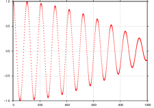
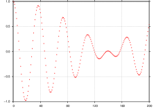
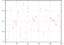
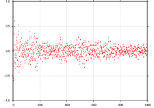
Figure 3. Numerically computed non-zero moments $(-1)^{k}c_{{3k}}^{(\theta)}$ for $\theta=30^{\circ}$, $50^{\circ}$ (top row), $70^{\circ}$ and $100^{\circ}$ (bottom row). The horizontal axis is $k$ and $\epsilon=10^{-10}$.

Figure 3 shows the numerically computed [6] moments for limit measures $\mu_{\theta}$ of different opening angles $\theta$. For clarity, we actually plotted $(-1)^{k}c_{3k}^{(\theta)}$, corresponding to the moments of $\mu_{\theta}$ rotated by $\pi$ [18, (1.6.63)]. For small $\theta$, the moments $c_{3j}^{(\theta)}$ appear to oscillate with a higher frequency with an amplitude modulated by another lower frequency. This is not unexpected since, for small $\theta$, the cells of the second generation are tiny. Since all points $z_{l}$ fall into these cells, the positions of the second generation cells control the general oscillation behaviour of the moments. As $\theta$ increases, the cells of every generation grow and the distances between successive cells of a given generation decreases, with higher-generation cells contributing different frequencies to the graph of the moments. The graph seems to become increasingly erratic.

4. Least eigenvalue of hyperbolic surfaces

4.1. Spectrum of $S_{d_{0},d_{1},d_{2}}$ and symmetries

Given three lengths $d_{0}$, $d_{1}$, $d_{2}>0$, there is (up to isometries) a unique genus-0 hyperbolic surface $S_{d_{0},d_{1},d_{2}}$ of infinite area with three cylindrical ends (funnels) whose short geodesics are of lengths $2d_{0}$, $2d_{1}$ and $2d_{2}$ [Fig. 4a]. Referring to Fig. 4b, this surface is the oriented double cover of $\mathbb{D}/\Gamma_{g_{0},g_{1},g_{2}}$, where $d_{j}$ is the hyperbolic distance between two geodesics. The three geodesics $g_{j}$, together with the geodesics realising the distances $d_{j}$, define a unique (up to isometries) hyperbolic right-angled hexagon. The three heights of this hexagon are concurrent [4, Thm. 2.4.3], and we choose their intersection point to be the origin of $\mathbb{D}$. The angle $\varphi$ and the hyperbolic length $t$ in Fig. 4b can be obtained using trigonometric identities for trirectangles and pentagons [4, Ch. 2], giving

$$\cos\varphi =\frac{\delta_{0}^{2}+\delta_{0}\delta_{1}\delta_{2}}{\sqrt{\delta_{0}^{2}+\delta_{1}^{2}+2\delta_{0}\delta_{1}\delta_{2}}\sqrt{\delta_{0}^{2}+\delta_{2}^{2}+2\delta_{0}\delta_{1}\delta_{2}}},$$ (21)

$$\tanh t =\delta_{0}\delta_{2}\sqrt{\frac{\delta_{0}^{2}+\delta_{1}^{2}+\delta_{2}^{2}+2\delta_{0}\delta_{1}\delta_{2}-1}{(\delta_{1}^{2}+\delta_{0}^{2}\delta_{2}^{2}+2\delta_{0}\delta_{1}\delta_{2})(\delta_{0}^{2}+\delta_{2}^{2}+2\delta_{0}\delta_{1}\delta_{2})}},$$

where $\delta_{j}=\cosh d_{j}$. The Euclidean distance from the origin of $\mathbb{D}$ is $x=\tanh(t/2)$. These results allow us to compute explicitly, for given distances $d_{0},d_{1},d_{2}$, the three primitive cells needed for McMullen’s algorithm.

\psfrag{g0}[c][c][0.707][0]{$g_{0}$}\psfrag{g1}[c][c][0.707][0]{$g_{1}$}\psfrag{g2}[c][c][0.707][0]{$g_{2}$}\psfrag{d0}[c][c][0.707][0]{$d_{0}$}\psfrag{2d0}[c][c][0.707][0]{$2d_{0}$}\psfrag{d1}[c][c][0.707][0]{$d_{1}$}\psfrag{2d1}[c][c][0.707][0]{$2d_{1}$}\psfrag{d2}[c][c][0.707][0]{$d_{2}$}\psfrag{2d2}[c][c][0.707][0]{$2d_{2}$}\psfrag{phi}[c][c][0.707][0]{$\varphi$}\psfrag{t}[c][c][0.707][0]{$t$}\psfrag{Sd0d1d2}[c][c][0.707][0]{$S_{d_{0},d_{1},d_{2}}$}\psfrag{(a)}{(a)}\psfrag{(b)}{(b)}\includegraphics[scale={0.3}]{surface.eps}

\psfrag{g0}[c][c][0.707][0]{$g_{0}$}\psfrag{g1}[c][c][0.707][0]{$g_{1}$}\psfrag{g2}[c][c][0.707][0]{$g_{2}$}\psfrag{d0}[c][c][0.707][0]{$d_{0}$}\psfrag{2d0}[c][c][0.707][0]{$2d_{0}$}\psfrag{d1}[c][c][0.707][0]{$d_{1}$}\psfrag{2d1}[c][c][0.707][0]{$2d_{1}$}\psfrag{d2}[c][c][0.707][0]{$d_{2}$}\psfrag{2d2}[c][c][0.707][0]{$2d_{2}$}\psfrag{phi}[c][c][0.707][0]{$\varphi$}\psfrag{t}[c][c][0.707][0]{$t$}\psfrag{Sd0d1d2}[c][c][0.707][0]{$S_{d_{0},d_{1},d_{2}}$}\psfrag{(a)}{(a)}\psfrag{(b)}{(b)}\includegraphics[scale={0.3}]{hexagon.eps}

Figure 4. (a) The hyperbolic surface $S_{d_{0},d_{1},d_{2}}$. (b) The corresponding hexagon with concurrent heights.

Let $D(d_{0},d_{1},d_{2}):=\Lambda_{\infty}(\Gamma_{g_{0},g_{1},g_{2}})$ denote the Hausdorff dimension of the limit set, and let $\lambda_{0}(S_{d_{0},d_{1},d_{2}})$ be the bottom of the spectrum of the (positive) Laplace operator on the surface $S_{d_{0},d_{1},d_{2}}$. The following result is well known and relates the above two functions. (The result holds generally for geometrically finite hyperbolic manifolds of infinite volume.)

Theorem 4.1.

[25, Thm. 2.21] We have, with the notions from above,

$$\lambda_{0}(S_{d_{0},d_{1},d_{2}})=\begin{cases}\frac{1}{4}&\text{if }D=D(d_{0},d_{1},d_{2})\leq\frac{1}{2},\\ \>D(1-D)&\text{if }D=D(d_{0},d_{1},d_{2})\geq\frac{1}{2},\end{cases}$$ (22)

and $\lambda_{0}(S_{l_{0},l_{1},l_{2}})<1/4$ is the eigenvalue of a positive $L^{2}$-eigenfunction if and only if $D(d_{0},d_{1},d_{2})>1/2$.

The spectral interpretation of the Hausdorff dimension was extended by Patterson in [16] (see also [3, Thm. 14.15]) to the case $D=D(d_{0},d_{1},d_{2})<1/2$, in which case $D$ represents the location of the first resonance.

Fixing a total distance $d>0$, we consider the function $(d_{0},d_{1},d_{2})\mapsto D(d_{0},d_{1},d_{2})$ with $d_{0}+d_{1}+d_{2}=d$. One might think that the point $p_{0}=(d/3,d/3,d/3)$ would be a unique global minimum of the Hausdorff dimension subject to this total distance restriction (in fact, this was our initial guess). Numerical computations showed, however, that the function $D(d_{0},d_{1},d_{2})$ is more complicated and has, in fact, precisely four global minima at $p_{0}$ and at $3$ other points,

$$\Bigl{(}\frac{2d}{3},\frac{d}{6},\frac{d}{6}\Bigr{)},\;\Bigl{(}\frac{d}{6},\frac{2d}{3},\frac{d}{6}\Bigr{)}\quad\textrm{and}\quad\Bigl{(}\frac{d}{6},\frac{d}{6},\frac{2d}{3}\Bigr{)}.$$

This observation lead to the following rigorous result:

Proposition 4.2.

Let $a,b>0$. Then we have

$$D(2b,a,a)=D(2a,b,b).$$ (23)

We note that Proposition 4.2 shows that, for $d>0$, the function $t\mapsto D(t,\frac{d-t}{2},\frac{d-t}{2})$ is symmetric with respect to $d/2$. In Fig. 1, this means that $D$ is symmetric about the midpoint along the line $AB$.

Proof.

The hexagon with the three geodesics $g_{0},g_{1},g_{2}$ with distances $a,a,2b$ is shown in Fig. 5b. The configuration is obviously symmetric with respect to the horizontal geodesic $g_{3}$. Let $\rho_{j}$ denote the hyperbolic reflection in $g_{j}$ and $D_{j}$ be the closed disk with $g_{j}=\partial D_{j}$. Then $\Gamma_{g_{0},g_{1},g_{2}}=\langle\rho_{0},\rho_{1},\rho_{2}\rangle=:\Gamma_{0}$, and a fundamental domain of $\Gamma_{0}$ is given by

$${\mathcal{F}}_{0}=\{z\in{\mathbb{C}}:\mathrm{Re}(z)>0\}\backslash(D_{0}\cup D_{2}).$$ (24)

The geodesic $g_{4}$ in Fig. 5b is the reflection of $g_{2}$ in $g_{1}$. Therefore, we have for the corresponding reflection $\rho_{4}=\rho_{1}\rho_{2}\rho_{1}$. A fundamental domain of $\widehat{\Gamma}=\langle\rho_{0},\rho_{1},\rho_{2},\rho_{3},\rho_{4}\rangle$ is

$$\widehat{\mathcal{F}}=\{z\in{\mathbb{C}}:\mathrm{Re}(z)>0,\;\mathrm{Im}(z)<0\}\backslash D_{2}.$$ (25)

Since ${\mathcal{F}}_{0}=\widehat{\mathcal{F}}\cup\rho_{3}(\widehat{\mathcal{F}})$ we have $[\widehat{\Gamma}:\Gamma_{0}]=2$. The geodesics $g_{2},g_{3},g_{4}$ in Fig. 5b have distances $b,b,2a$. Completely analogously, noting that $\Gamma_{g_{2},g_{3},g_{4}}=\langle\rho_{2},\rho_{3},\rho_{4}\rangle=:\Gamma_{1}$ has

$${\mathcal{F}}_{1}=\{z\in{\mathbb{C}}:\mathrm{Im}(z)<0\}\backslash(D_{2}\cup D_{4})$$ (26)

as a fundamental domain, we have $\rho_{0}=\rho_{3}\rho_{2}\rho_{3}$, and ${\mathcal{F}}_{1}=\widehat{\mathcal{F}}\cup\rho_{1}(\widehat{\mathcal{F}})$. This implies, again, $[\widehat{\Gamma}:\Gamma_{1}]=2$ and, therefore,

$$\mathrm{dim}_{H}\Lambda_{\infty}(\Gamma_{0})=\mathrm{dim}_{H}\Lambda_{\infty}(\Gamma_{1})=\mathrm{dim}_{H}\Lambda_{\infty}(\widehat{\Gamma}).$$ (27)

\psfrag{D0}[c][c][0.707][0]{$D_{0}$}\psfrag{D1}[c][c][0.707][0]{$D_{1}$}\psfrag{D2}[c][c][0.707][0]{$D_{2}$}\psfrag{D3}[c][c][0.707][0]{$D_{3}$}\psfrag{D4}[c][c][0.707][0]{$D_{4}$}\psfrag{D5}[c][c][0.707][0]{$D_{5}$}\psfrag{g0}[c][c][0.707][0]{$g_{0}$}\psfrag{g1}[c][c][0.707][0]{$g_{1}$}\psfrag{g2}[c][c][0.707][0]{$g_{2}$}\psfrag{g3}[c][c][0.707][0]{$g_{3}$}\psfrag{g4}[c][c][0.707][0]{$g_{4}$}\psfrag{g5}[c][c][0.707][0]{$g_{5}$}\psfrag{a}[c][c][0.707][0]{$a$}\psfrag{b}[c][c][0.707][0]{$b$}\psfrag{2a}[c][c][0.707][0]{$2a$}\psfrag{2b}[c][c][0.707][0]{$2b$}\psfrag{4a}[c][c][0.707][0]{$4a$}\psfrag{4b}[c][c][0.707][0]{$4b$}\psfrag{(a)}{(a)}\psfrag{(b)}{(b)}\psfrag{(c)}{(c)}\psfrag{alpha}[c][c][0.707][0]{$\alpha$}\psfrag{beta}[c][c][0.707][0]{$\beta$}\includegraphics[width=433.62pt]{funddoms.eps}

Figure 5. Surfaces: (a) $S_{2a,b,b}$ and (c) $S_{2b,a,a}$. (b) The associated domains in $\mathbb{D}$.

∎

Remark.

The spectrum of a geometrically finite hyperbolic surface of infinite area consists of an absolutely continuous part $[1/4,\infty)$ without embedded eigenvalues and finitely many eigenvalues of finite multiplicity in the interval $(0,1/4)$; see [8, 9, 10, 11] or [3, Ch. 7].

Assuming $D(2a,b,b)>1/2$, we conclude from Thm. 4.1 and Prop. 4.2 that $\lambda_{0}(S_{2a,b,b})=\lambda_{0}(S_{2b,a,a})$, i.e. $S_{2a,b,b}$ and $S_{2b,a,a}$ have the same lowest eigenvalue. It is natural to ask whether these two surfaces are isospectral. We obtain $S_{2b,a,a}$ from $S_{2a,b,b}$ by first cutting $S_{2a,b,b}$ along the geodesics $\alpha$, $\beta$ in Fig. 5a, unfolding it onto $\mathbb{D}\backslash(D_{0}\cup D_{2}\cup D_{4}\cup D_{5})\allowbreak=:D_{S}$ in Fig. 5b, and then gluing the boundary geodesics $g_{0},g_{5}$ and $g_{2},g_{4}$ together. Let $\rho_{j}$ be the reflection along geodesic $g_{j}$ as before, with $\rho_{1},\rho_{3}$ also considered to act isometrically on $S_{2a,b,b}$ and $S_{2b,a,a}$. Since $\rho_{1}$, $\rho_{3}$ and the Laplacian $\Delta$ commute, we consider simultaneous eigenfunctions of these operators on $S_{2a,b,b}$. Let $f$ be an $L^{2}$-eigenfunction in $S_{2a,b,b}$ with eigenvalue $\lambda<1/4$ which is even under $\rho_{1}$ and $\rho_{3}$,

$$\Delta f=\lambda f\qquad\textrm{with}\quad f\circ\rho_{1}=f=f\circ\rho_{3}.$$ (28)

(At least one such $f$ exists—with $\lambda=\lambda_{0}$.) Now any such $f\in C^{\infty}(S_{2a,b,b})$ can be transplanted to $\widetilde{f}\in C^{\infty}(D_{S})$. Thanks to the symmetry (28b), $\widetilde{f}$ along with all its derivatives agree along the corresponding points on $g_{0},g_{5}$ and $g_{2},g_{4}$, so $\widetilde{f}$ can in turn be transplanted to an $L^{2}$-eigenfunction $\hat{f}\in C^{\infty}(S_{2b,a,a})$ with the same eigenvalue, $\Delta\hat{f}=\lambda\hat{f}$ in $S_{2b,a,a}$. One can carry out the same argument when $f\circ\rho_{1}=-f=f\circ\rho_{3}$ in (28), assuming such an $f$ exists. This argument shows that some eigenvalues of these two surfaces coincide.

4.2. Example $S_{d_{0},d_{1},d_{2}}$ with $d_{0}+d_{1}+d_{2}=3$

Identifying the triple $(d_{0},d_{1},d_{2})$ with the point $(d_{0}+d_{1}\mathrm{e}^{2\pi\mathrm{i}/3}+d_{2}\mathrm{e}^{4\pi\mathrm{i}/3})\,\mathrm{i}/\sqrt{3}\in{\mathbb{R}}^{2}$, we represent the domain of $D(d_{0},d_{1},d_{2})$ by an equilateral triangle $\mathcal{T}\subset{\mathbb{R}}^{2}$ centred at $0$ with heights $\sqrt{3}/2$; see Fig. 1. In Fig. 6 we plot $D(d_{0},d_{1},d_{2})$ restricted to $d_{0}+d_{1}+d_{2}=3$, computed using McMullen’s algorithm. When any $d_{j}$ is small (i.e. for points close to $\partial\mathcal{T}$), it is difficult to compute $D$ numerically using McMullen’s algorithm even with $256$-bit arithmetic; we have therefore left out the blank regions near $\partial\mathcal{T}$ (thick black triangle on the plot).

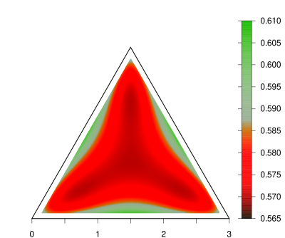
Figure 6. Graph of the function $D(d_{0},d_{1},d_{2})$ restricted to $d_{0}+d_{1}+d_{2}=3$; bottom axis is $d_{1}$ with $d_{0}=0$.

We found the minimum of $D$ to be $D(1,1,1)\doteq 0.56996\ldots>1/2$, which as noted above is also attained at three other points $(2,1/2,1/2)$, $\ldots$. We remark that $D$ is very flat for much of $\mathcal{T}$ (red region in the plot), only increasing rapidly near $\partial\mathcal{T}$ (where our numerical computation breaks down). The four global minima of $D$ can also be seen in Fig. 7, which shows the bottom of $D$ at an expanded vertical scale. In view of the apparent smoothness of the function $D$ in Fig. 7, it is natural to ask whether there are explicit formulas for the gradient or the Hessian of $D$. From the shape of the graph (the part reliably computed), we believe that $D$ attains its global maximum at the vertices and the midpoints of $\partial\mathcal{T}$.

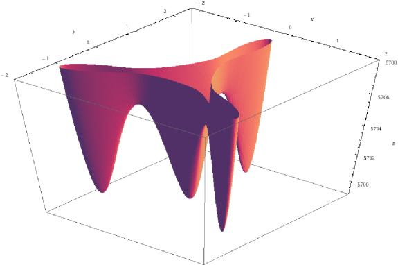
Figure 7. The bottom part of $D(d_{0},d_{1},d_{2})$; note scale.

The value of $D$ at these points can be computed using (23) and the results of Baragar [1], who described an algorithm for the Hausdorff dimension of reflection groups $\Gamma_{g_{0},g_{1},g_{2}}$ with two distances equal to zero. Our $(d_{0},d_{1},d_{2})=(3,0,0)$ corresponds to $a=(1+x)/(1-x)\doteq 2.35240\ldots$ in [1] with $x=\tanh^{2}(3/4)$. Using [1, Table 1], we obtain $0.225<\lambda_{0}(S_{3,0,0})<0.226$ and consequently $0.654<D(3,0,0)=D(0,3/2,3/2)<0.659$, which we believe bounds the global maximum of $D$ in $\mathcal{T}$.

Remark.

Our numerical computations indicate that the situation does not change qualitatively when we choose a much larger total distance $d$ (we also carried out detailed calculations for the case $d=6$ with the global minimum $0.334541\ldots$, and obtained graphs very similar to Figs. 6 and 7). For any $\epsilon\in(0,\epsilon_{0})$, there exists a total distance $d=d(\epsilon)$ such the four global minima of $D$ under the restriction $d_{0}+d_{1}+d_{2}=d$ agree with $\epsilon$. Again, for a large part of $\mathcal{T}$, the graph of $D$ should be relatively flat.

It seems plausible and there is strong numerical evidence (although we do not have a proof) that one has

$$D(d_{0},d_{1},d_{2})\leq D(d_{0}^{\prime},d_{1}^{\prime},d_{2}^{\prime})\quad\textrm{if }d_{j}^{\prime}\leq d_{j}\textrm{ for }j=0,1,2.$$ (29)

Assuming continuity of $D$ up to the boundary $\partial\mathcal{T}$, the graph must become very steep close to the boundary, because McMullen’s asymptotic $\lim_{c\to\infty}D(c,c,0)=1/2$ [12, Thm. 3.6], together with the monotonicity property (29), imply that $D$ assumes values $\geq 1/2$ at all boundary points $\partial\mathcal{T}$: For $(a,b,0)\in\partial\mathcal{T}$ with $a>b>0$ we have

$$D(a,b,0)\geq D(a,a,0)\geq\lim_{c\to\infty}D(c,c,0)=1/2.$$ (30)

5. OPUC and CMV matrices

5.1. Overview

We review briefly the properties of OPUCs and CMV matrices as relevant to the current work, referring the reader to [18, 19, 20, 21] for more details. As before, $\mathbb{D}\subset{\mathbb{C}}$ denotes the open unit disk and $S^{1}=\partial\mathbb{D}$. Given a probability measure $\mu$ on $S^{1}$, supported on an infinite set, and the inner product (14), let $\{\Phi_{k}(z;\mu)\}_{k=0}^{\infty}$ be a set of monic polynomials orthogonal with respect to $\mu$ (with the usual convention that $\Phi_{k}(z;\mu)=z^{k}+{}$lower-order terms); for brevity, we will often write $\Phi_{k}(z)$ for $\Phi_{k}(z;\mu)$ when there is no confusion. As do real orthogonal polynomials, $\{\Phi_{k}\}$ satisfy a recurrence relation

$$\Phi_{k+1}(z)=z\Phi_{k}(z)-\bar{\alpha}_{k}\Phi_{k}^{*}(z)$$ (31)

called Szegő’s recursion, where the Verblunsky coefficients $\alpha_{k}$ can be shown to lie in $\mathbb{D}$. The reversed polynomial is

$$\Phi_{k}^{*}(z):=z^{k}\overline{\Phi_{k}(1/\bar{z})}$$ (32)

or, with $\Phi_{k}(z)=\sum_{j=0}^{k}\,b_{j}z^{j}$,

$$\Phi_{k}^{*}(z)=\textstyle\sum_{j=0}^{k}\,\bar{b}_{k-j}z^{j}.$$ (33)

This implies that $\Phi_{k}^{*}(0)=1$ for all $k$ and, together with (31),

$$\alpha_{k}=-\overline{\Phi_{k+1}(0)}.$$ (34)

In practice, one can compute $\{\Phi_{k}\}_{k=0}^{\infty}$ using Gram–Schmidt on $\{z^{k}\}_{k=0}^{\infty}$. We note that $\{\Phi_{k}\}$ may or may not form a basis for $L^{2}(S^{1};\mu)$; see [20, Thm. 2.2].

If, on the other hand, we apply Gram–Schmidt to $\{1,z,z^{-1},z^{2},z^{-2}$, $\ldots\}$, we get orthonormal polynomials $\{\chi_{0}(z),\chi_{1}(z),\chi_{2}(z),\ldots\}$ which do form a basis for $L^{2}(S^{1};\mu)$. The CMV matrix associated to the measure $\mu$ is the matrix representation of the operator $f(z)\to zf(z)$ on $L^{2}(S^{1};\mu)$. It has the semi-infinite pentadiagonal form

$${\mathcal{C}}=\left(\begin{array}[]{cccccc}\bar{\alpha}_{0}&\bar{\alpha}_{1}\rho_{0}&\rho_{1}\rho_{0}&0&0&\ldots\\ \rho_{0}&-\bar{\alpha}_{1}\alpha_{0}&-\rho_{1}\alpha_{0}&0&0&\ldots\\ 0&\bar{\alpha}_{2}\rho_{1}&-\bar{\alpha}_{2}\alpha_{1}&\bar{\alpha}_{3}\rho_{2}&\rho_{3}\rho_{2}&\ldots\\ 0&\rho_{2}\rho_{1}&-\rho_{2}\alpha_{1}&-\bar{\alpha}_{3}\alpha_{2}&-\rho_{3}\alpha_{2}&\ldots\\ 0&0&0&\bar{\alpha}_{4}\rho_{3}&-\bar{\alpha}_{4}\alpha_{3}&\ldots\\ \vdots&\vdots&\vdots&\vdots&\vdots&\ddots\\ \end{array}\right)$$ (35)

where $\rho_{k}=\sqrt{1-|\alpha_{k}|^{2}}$. We note that Jacobi matrices, obtained in a similar way for orthogonal polynomials on the real line, are tridiagonal matrices. As in the case of orthogonal polynomials on the real line, an important connection between CMV matrices and monic orthogonal polynomials is

$$\Phi_{n}(z)=\operatorname*{det}(zI-{\mathcal{C}}^{(n)})$$ (36)

where ${\mathcal{C}}^{(n)}$ is the upper left $n\times n$ corner of ${\mathcal{C}}$.

If $|\alpha_{n-1}|=1$, ${\mathcal{C}}$ decouples between $(n-1)$ and $n$ as ${\mathcal{C}}={\mathcal{C}}^{(n)}\oplus\tilde{{\mathcal{C}}}$, where the upper left corner is an $n\times n$ unitary matrix ${\mathcal{C}}^{(n)}={\mathcal{C}}^{(n)}(\alpha_{0},\alpha_{1},\ldots,\alpha_{n-1})$ and the remaining block $\tilde{\mathcal{C}}(\alpha_{n},\alpha_{n+1},\ldots)$ is a (semi-infinite) CMV matrix. This suggests that a unitary $n\times n$ truncation of a CMV matrix can be obtained by replacing $\alpha_{n}\in\mathbb{D}$ by $\beta\in\partial\mathbb{D}$. The truncated CMV matrix has as characteristic polynomial

$$\Phi_{n}(z;\beta)=z\Phi_{n-1}(z)-\beta\Phi_{n-1}^{*}(z)$$ (37)

whose zeros are all simple and lie on $\partial\mathbb{D}=S^{1}$, a fact which will be convenient below. The polynomials $\Phi_{n}(z;\beta)$ are called paraorthogonal polynomials.

Given a set of moments $c_{k}(\mu)$, we can recover its generating measure $\mu$ in the classical limit as follows [18, Thm. 2.2.12]. Given $\beta$ and $k$, let $\{z_{j}\}_{j=1}^{k}\subset\partial\mathbb{D}$ be the zeros of $\Phi_{k}(z;\beta)$ and define the atomic measure

$$\zeta^{(k)}_{\beta}:=\sum_{j=1}^{k}\frac{1}{\sum_{i=0}^{k-1}\,|\varphi_{i}(z_{j})|^{2}}\delta_{z_{j}}$$ (38)

where $\varphi_{i}(z)=\Phi_{i}(z)/\|\Phi_{i}\|$, and $\|\cdot\|$ denotes the norm in $L^{2}(S^{1};\mu)$. For any choice of $\beta_{1},\beta_{2},\beta_{3},\ldots\in\partial\mathbb{D}$, $\zeta^{(k)}_{\beta_{k}}$ converges weakly to $\mu$. The weight $\bigl{(}\sum_{i}\,|\varphi_{i}(z_{j})|^{2}\bigr{)}^{-1}$ is known as the Christoffel function [18, p. 117ff].

5.2. OPUCs for SPP

Let us now return to McMullen’s SPP. Using the moments $c_{{k}}^{(\theta)}$ computed in Section 3.3, we used Gram–Schmidt to construct the orthogonal polynomials $\Phi_{k}(z)=\Phi_{k}(z;\mu_{\theta})$ associated to the measure $\mu_{\theta}$, which for convenience we rotate by $\pi$. Henceforth, by $\mu_{\theta}$ we mean this rotated measure. Since all moments are real and $c_{{3k-1}}^{(\theta)}=c_{{3k+1}}^{(\theta)}=0$, the polynomials $\Phi_{3k}(z)$ are, in fact, polynomials in $z^{3}$ with real coefficients, and $\Phi_{3k+1}(z)=z\Phi_{3k}(z)$ and $\Phi_{3k+2}(z)=z^{2}\Phi_{3k}(z)$. It then follows from (34) that the Verblunsky coefficients are all real with $\alpha_{3k}=\alpha_{3k+1}=0$ and $\alpha_{3k+2}\in(-1,1)$; this also follows from the symmetries of $\mu$ and [18, (1.6.66)].

It is convenient to introduce monic polynomials $q_{k}(z^{3}):=\Phi_{3k}(z)$ with Verblunsky coefficients $\gamma_{k}:=\alpha_{3k+2}$, in terms of which (31) reads

$$q_{k+1}(z)=zq_{k}(z)-\gamma_{k}q_{k}^{*}(z).$$ (39)

In analogy with (37), we define the paraorthogonal

$$q_{k}(z;\beta)=zq_{k-1}(z)-\beta q_{k-1}^{*}(z),$$ (40)

where we choose now $\beta=\pm 1$ depending on the sign of $\gamma_{k-1}$. Since $q_{k}(z^{3};\beta)=\Phi_{3k}(z;\beta)$, the zeros of $q_{k}(z;\beta)$ all lie on $\partial\mathbb{D}$. Moreover, since $q_{k}$ has real coefficients, its (non-real) zeros occur in complex conjugate pairs. For our numerical computations, we used $q_{k}$ exclusively in place of $\Phi_{3k}$. Since the OPUCs depend on the underlying measure $\mu$ only through the moments $c_{j}$, it is clear from the definition (15) of the latter that $\{q_{k}\}_{k=0}^{\infty}$ are the OPUCs for a measure $\tilde{\mu}_{\theta}$ where

$$\mathrm{d}\tilde{\mu}_{\theta}(\phi)=3\,\mathrm{d}\mu_{\theta}(\phi/3)$$ (41)

for $\phi\in[-\pi/3,\pi/3)$.

Having computed $q_{k}$ and $\gamma_{k}=-q_{k+1}(0)$, the accuracy of the numerical computation can be checked using (31), by ensuring that the error (which is zero for exact computation)

$$\mathcal{E}_{k}:=\textstyle\sum_{j}\,|q_{k+1,j}-q_{k,j-1}+\gamma_{k}q_{k,k-j}|,$$

with $q_{k,j}$ the $j$th coefficient of $q_{k}$ (with $q_{k,-1}=0$), remains small. We found that high-precision arithmetic, both for the moments $c_{k}$ and the subsequent computations involving $q_{k}$, are crucial to control the error. For $\theta=119^{\circ}$ and $\epsilon=10^{-7}$, computations using a 256-bit “quad-double” precision gives us $k\simeq 280$.

5.3. Observations

We now present a few numerical observations on the spectral properties of CMV matrices. In this section, we work exclusively with the symmetry-reduced polynomials $q_{k}$ and the measure $\tilde{\mu}_{\theta}$ introduced above.

First, for every $\theta\in(0,2\pi/3)$, the Verblunsky coefficients are all negative, $\gamma_{k}<0$. Seen in the light of the formula for Verblunsky coefficients for rotated measures [18, (1.6.66)], for any measure $\mu$,

$$\gamma_{k}(\mu^{(\alpha)})=\mathrm{e}^{-\mathrm{i}\alpha(k+1)}\,\gamma_{k}(\mu)$$ (42)

where $\mathrm{d}\mu^{(\alpha)}(\phi)=\mathrm{d}\mu(\phi-\alpha)$, our observation means that $\mu_{\theta}$ belongs to a family of measures whose Verblunsky coefficients are, possibly after rotation, all negative. To obtain paraorthogonal polynomials $q_{k}(z;\beta)$ corresponding to unitary truncations of the CMV matrix, it is therefore natural to take $\beta=-1$ (but see the effect of the choice of $\beta$ at the end of this section).

\psfrag{ 120}[c][c][0.707][0]{$\theta$}\psfrag{yyy}[r][r][0.707][0]{$\log(1+\gamma_{k})$}\includegraphics[scale={0.40},angle={-90}]{nverb.ps}

Figure 8. Monotonicity of Verblunsky coefficients: Plot of $\log(1+\gamma_{k})$ against $\theta$ for (from top) $k=1,2,4$.

Secondly, for every $k$ fixed, $\gamma_{k}(\mu_{\theta})$ increases monotonically from $-1$ to $0$ as $\theta$ goes from $0$ to $2\pi/3$. Figure 8 plots $\log(1+\gamma_{k})$ for $k=1$, $2$ and $4$ against $\theta$, showing the rapid convergence of $\gamma_{k}$ to $-1$ as $\theta\to 0$.

In the course of our numerical computations, we found that small opening angles $\theta$ only allow us to obtain a few polynomials $q_{k}$ reliably, while larger $\theta$ allows us to obtain more polynomials. Since the numerical instability of the Gram-Schmidt orthogonalisation of the polynomials $1,z,z^{2},\ldots$ is closely related to the numerical singularity of the Toeplitz matrices

$$T^{(n+1)}_{\theta}=(c_{j-i}^{(\theta)})_{0\leq i,j\leq n}=(\langle z^{j},z^{i}\rangle_{\theta})_{0\leq i,j\leq n},$$ (43)

we expect that the determinant $D_{n}(d\mu_{\theta}):=\operatorname*{det}T^{(n+1)}_{\theta}$ decreases monotonically to $0$ as $\theta\to 0$. In fact, this would follow from the monotonicity of the individual Verblunsky coefficients by the identity [18, §1.3.2 and (2.1.1)]

$$D_{n}(d\mu_{\theta})=\prod_{j=0}^{n-1}\,(1-|\gamma_{j}(\mu_{\theta})|^{2})^{n-j}.$$ (44)

\psfrag{phi}[c][c][0.707][0]{$\phi$}\psfrag{pi}[c][c][0.707][0]{$\pi$}\psfrag{ 1}[r][r][0.707][0]{$1$}\includegraphics[scale={0.45},angle={-90}]{w119.ps}

Figure 9. Solid (green) line: (classical) measure $\mu_{119}$, red dots (overlapping the line): $\zeta^{(280)}$, blue dots: $\mathrm{idz}^{(280)}$.

In Figure 9, we present our numerical computations for $\theta=119^{\circ}$ with $\epsilon=10^{-7}$ (size of the largest cell). The thin (green) line is the distribution function of the classical measure $\tilde{\mu}_{119}([0,\phi])$. As noted earlier, $\mathrm{d}\tilde{\mu}_{\theta}$ tends to the Lebesgue measure $\mathrm{d}\phi/(2\pi)$ as $\theta\to 120^{\circ}$, but significant “gaps” (i.e. intervals $I$ with $\tilde{\mu}(I)=0$) remain even for $\theta=119^{\circ}$. Let $z_{j}$ be the zeros of the paraorthogonal $q_{280}(z;\beta\!=\!-1)$, ordered from $\phi=0$ to $2\pi$. The blue dots in Fig. 9 plot the “integrated density of zeros” measure

$$\mathrm{idz}^{(k)}=\sum\nolimits_{j=1}^{k}\,\frac{1}{k}\delta_{z_{j}},$$ (45)

while the red dots plot the “Christoffel-corrected” measure $\zeta^{(280)}$ defined in (38). One can see that $\zeta^{(280)}$ overlaps the classical measure $\tilde{\mu}_{119}$ to within plotting line thickness. This agreement confirms the accuracy of our numerical computations. We note that one may find zeros in the spectral gaps $S^{1}\backslash\mathrm{supp}\,\mu_{\theta}$, but with smaller probability as $k\to\infty$ and the Christoffel function at these “spurious” zeros is small.

The idz plot also suggests that in the limit $k\to\infty$, zeros appear to accumulate at the gap edges, most visibly for the main gap centred at $0=2\pi$ and the secondary gap starting at $\pi$. As noted above, there could be zeros inside the gaps; here they are most visible near $2\pi/3$ and $4\pi/3$ [see also Fig. 10 below]. However, their contribution to the measure $\zeta^{(k)}$ is weighted down by the Christoffel function.

\psfrag{arg(zk)}[c][c][0.707][0]{arg$\,z_{k}$}\psfrag{pi}[c][c][0.707][0]{$\pi$}\psfrag{arg(B)}[r][r][0.707][0]{arg$\,\beta$}\includegraphics[scale={0.45},angle={-90}]{cc119.ps}

Figure 10. Migration of zeros of $q_{40}(z;\beta)$ as a function of $\beta$ for $\theta=119^{\circ}$. Horizontal axis is arg$\,z_{k}$ and the vertical axis is arg$\,\beta$. Each vertical “line” is in fact made up of 500 disjoint dots. Faint (green) background is the approximate support of the classical measure $\mu_{119}$.

In Figure 10, we plot, for $\theta=119^{\circ}$ and $\beta\in S^{1}$, the migration of the zeros of $q_{40}(z;\beta)$ as arg$\,\beta$ varies from $0$ to $2\pi$, superimposed on the support of the classical measure $\mu_{119}$ (since supp$\,\mu_{119}$ has Lebesgue measure zero, the “solid” background arises only from plotting limitations). This plot confirms Thm. 1.1 in [22], which states that any interval $[a,b]\not\in\textrm{supp}\,\mu$, represented by a white background, contains at most one zero of $q(z;\mu,\beta)$. It also confirms Thm. 1.3 in [22], stating that for any $\beta$, $\beta^{\prime}\in S^{1}$, the zeros of $q_{k}(z;\beta)$ and of $q_{k}(z;\beta^{\prime})$ strictly interlace. The graph also shows that each zero $z_{k}^{(\beta)}$ is monotone in arg$\,\beta$ and travels from $z_{k}^{(0)}$ to $z_{k+1}^{(0)}$ as arg$\,\beta$ increases from $0$ to $2\pi$.

References

- [1] A. Baragar, Fractals and the base eigenvalue of the Laplacian on certain noncompact surfaces, Experimental Math., 15 (2006), pp. 33–42.
- [2] A. F. Beardon, The geometry of discrete groups, Springer-Verlag, 1983.
- [3] D. Borthwick, Spectral theory of infinite-area hyperbolic surfaces, Birkhäuser, 2007.
- [4] P. Buser, Geometry and spectra of compact Riemann surfaces, Birkhäuser, 2010.
- [5] M. J. Cantero, L. Moral, and L. Velázquez, Five-diagonal matrices and zeros of orthogonal polynomials on the unit circle, Linear Alg. Appl., 362 (2003), pp. 29–56.
- [6] K. Gittins, N. Peyerimhoff, M. Stoiciu, and D. Wirosoetisno, some codes for the computations in this article are filed as ancillary files of arXiv:1112.1020.
- [7] O. Jenkinson and M. Pollicott, Calculating Hausdorff dimension of Julia sets and Kleinian limit sets, Amer. J. Math., 124 (2002), pp. 495–545.
- [8] P. D. Lax and R. S. Phillips, The asymptotic distribution of lattice points in Euclidean and non-Euclidean spaces, J. Funct. Anal., 46 (1982), pp. 280–350.
- [9] P. D. Lax and R. S. Phillips, Translation representation for automorphic solutions of the wave equation in non-Euclidean spaces. I, Comm. Pure Appl. Math., 37 (1984), pp. 303–328.
- [10] , Translation representations for automorphic solutions of the wave equation in non-Euclidean spaces. II, Comm. Pure Appl. Math., 37 (1984), pp. 779–813.
- [11] , Translation representations for automorphic solutions of the wave equation in non-Euclidean spaces. III, Comm. Pure Appl. Math., 38 (1985), pp. 179–207.
- [12] C. T. McMullen, Hausdorff dimension and conformal dynamics III: computation of dimension, Amer. J. Math., 120 (1998), pp. 691–721.
- [13] , Hausdorff dimension and conformal dynamics I: strong convergence of Kleinian groups, J. Diff. Geom., 51 (1999), pp. 471–515.
- [14] P. J. A. Nicholls, A measure on the limit set of a discrete group, in Ergodic theory, symbolic dynamics, and hyperbolic spaces (Trieste, 1989), T. Bedford, M. Keane, and C. Series, eds., Oxford Univ. Press, 1991, pp. 259–297.
- [15] S. J. Patterson, The limit set of a Fuchsian group, Acta Math., 136 (1976), pp. 241–273.
- [16] , On a lattice-point problem in hyperbolic space and related questions in spectral theory, Ark. Mat., 26 (1988), pp. 167–172.
- [17] R. Phillips and P. Sarnak, The Laplacian for domains in hyperbolic space and limit sets of Kleinian groups, Acta Math., 155 (1985), pp. 173–241.
- [18] B. Simon, Orthogonal polynomials on the unit circle, part 1: classical theory, American Math. Soc., 2004.
- [19] , Orthogonal polynomials on the unit circle, part 2: spectral theory, American Math. Soc., 2004.
- [20] , OPUC on one foot, Bull. Amer. Math. Soc., 42 (2005), pp. 431–460.
- [21] , CMV matrices: five years after, J. Comput. Appl. Math., 208 (2007), pp. 120–154.
- [22] , Rank one perturbations and the zeros of paraorthogonal polynomials on the unit circle, J. Math. Anal. Appl., 329 (2007), pp. 376–382.
- [23] D. Sullivan, The density at infinity of a discrete group of hyperbolic motions, Inst. Hautes Études Sci. Publ. Math., 50 (1979), pp. 171–202.
- [24] , Entropy, Hausdorff measures old and new, and limit sets of geometrically finite Kleinian groups, Acta Math., 253 (1984), pp. 259–277.
- [25] , Related aspects of positivity in Riemannian geometry, J. Diff. Geom., 25 (1987), pp. 327–351.