Twitter reciprocal reply networks exhibit assortativity with respect to happiness

Abstract

The advent of social media has provided an extraordinary, if imperfect, big data window into the form and evolution of social networks. Based on nearly 40 million message pairs posted to Twitter between September 2008 and February 2009, we construct and examine the revealed social network structure and dynamics over the time scales of days, weeks, and months. At the level of user behavior, we employ our recently developed hedonometric analysis methods to investigate patterns of sentiment expression. We find users average happiness scores to be positively and significantly correlated with those of users one, two, and three links away. We strengthen our analysis by proposing and using a null model to test the effect of network topology on the assortativity of happiness. We also find evidence that more well connected users write happier status updates, with a transition occurring around Dunbar’s number. More generally, our work provides evidence of a social sub-network structure within Twitter and raises several methodological points of interest with regard to social network reconstructions.

1 Introduction

Social network analysis has a long history in both theoretical and applied settings [1]. During the last 15 years, and driven by the increased availability of real-time, in-situ data reflecting people’s social interactions and choices, there has been an explosion of research activity around social phenomena, and many new techniques for characterizing large-scale social networks have emerged. Numerous studies have examined the structure of online social networks in particular, such as blogs, Facebook, and Twitter [2, 3, 4, 5, 6, 7, 8, 9, 10, 11, 12, 13, 14, 15, 16, 17, 18, 19].

In a series of analyses of the Framingham Heart Study data and the National Longitudinal Study of Adolescent Health, Christakis, Fowler, and others have examined how qualities such as happiness, obesity, disease, and habits (e.g., smoking) are correlated within social network neighborhoods [20, 21, 22, 23, 24, 25]. The authors’ additional assertion of contagion, however, has been criticized primarily on the basis of the difficulties to be found in distinguishing these phenomena from homophily [26, 27, 28]. The observation that social networks exhibit assortativity with respect to these traits evidently requires further study and leads us to explore potential mechanisms. Advances would naturally provide further insight into the nature of how social groups influence individual behavior and vice versa.

Our focus in the present work is the social network of Twitter users. With the abundance of available data, Twitter serves as a living laboratory for studying contagion and homophily [29]. As a requisite step towards these goals, we first define sub-networks of Twitter users suitable to such study and, second, examine whether assortativity is observed in these sub-networks. Before describing our methods, we provide a brief overview of Twitter, related work, and the challenges associated with social network analysis in this arena.

Twitter is an online, interactive social media platform in which users post tweets, micro-blogs with a 140 character limit. Since its inception in 2006, Twitter has grown to encompass over 200 million accounts, with over 100 million of these accounts currently active as of October 2011, and with some users having garnered over 10 million followers [30]. Tweets are open online by default, and are also broadcast directly to a user’s followers. Users may express interest in a tweet by retweeting the message to their followers. Alternatively, followers may reply directly to the author.

Understanding the topology of the Twitter network, the manner in which users interact and the diffusion of information through this media is challenging, both computationally and theoretically. One of the central issues in characterizing the topology of any network representation of Twitter lies in defining the criteria for establishing a link between two users. The majority of previous studies have examined the topology of and information cascades on the Twitter follower network [7, 10, 15], as well as on networks derived from mutual following [8]. However, the follower network is not the only representation of Twitter’s social network, and its structure can be misleading [31]. For example, in a study of over 6 million users, Cha et al. [10] found that users with the highest follower counts were not the users whose messages were most frequently retweeted. This suggests that such popular users (as measured by follower count) may not be the most influential in terms of spreading information, and this calls into question the extent to which users are influenced by those that they follow [32]. Of further concern is the finding of low reciprocity within follower networks. Kwak et al. found very few individuals who followed their followers [15]. As a result, trying to infer meaningful influence and contagion in such a network is difficult.

(a) Followers

(b) Interaction

Figure 1: (a) Follower network: The follower network is generated by declared following choices, absent any messages being sent. If user $v_{i}$ broadcasts tweets to followers $v_{j},v_{k}$ and $v_{\ell}$ (represented by the dashed, blue arrow) $v_{i}$ would be connected to each of $v_{j},v_{k}$ and $v_{\ell}$ by a directed link in a follower network. (b) Reciprocal-reply network: Directed replies are represented by a solid black arrow. When considering the interaction between users, a reply (i.e., $v_{\ell}$ replies to $v_{i}$) provides evidence of a directional interaction between nodes. We mandate a stronger condition for interaction, namely reciprocal replies (i.e., $v_{j}$ replies to $v_{i}$ and vice versa) over a given time period. Thus $v_{i}$ and $v_{j}$ are connected in the reciprocal reply network that we construct.

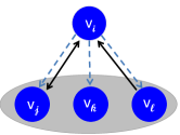
While popular users and their many followers clearly exhibit an affiliation, they do not necessarily interact, as there are different relationships implicated by broadcasting (tweeting), sending a message (@someone), and replying to a message. As an example, we consider a user represented by node $v_{i}$ which has three followers, represented by $v_{j},v_{k},$ and $v_{\ell}$ as shown in Fig. 1a. When a user broadcasts tweets to their many followers, as represented by the directed arrow in Fig. 1a, this does not imply that followers read or respond to these tweets. Followers $v_{j},v_{k},$ and $v_{\ell}$ receive all tweets broadcast by node $v_{i}$, but this provides no guarantee of interaction. Suppose, though, that we observe that $v_{\ell}$ replies to $v_{i}$ as shown in Figure 1b. This provides evidence (but not proof) that the user represented by $v_{\ell}$ has indeed received a tweet from $v_{i}$ and is sufficiently motivated to create a response to $v_{i}$. Although a directional network based on these replies can be created, such a directional interaction, however, does not suggest reciprocity between the nodes. In this example, we have no evidence that $v_{i}$ has, in any way, considered or even read such a response from his/her follower.

We conclude that following and unreciprocated replies are not sufficient for interaction and present an alternative means by which to derive a social network from Twitter messages, via reciprocal replies. In our reciprocal-reply network, two nodes, $v_{i}$ and $v_{j}$, are connected if $v_{i}$ has replied to $v_{j}$ and $v_{j}$ has replied to $v_{i}$ at least once within a given time period of consideration. In Figure 1b, the nodes $v_{i}$ and $v_{j}$ meet this criterion.

Another challenge in characterizing the topology of any network representation of Twitter concerns determining how long a link between two users in the network should persist. Including stale user-user interactions in the network mistakenly creates an inaccurate portrayal of the current state of the system; this is typically referred to as the “unfriending problem” [26]. Not only will network statistics such as the number of nodes, average degree, maximum degree and proportion of nodes in the giant component be artificially inflated due to superfluous, no-longer-active links [26, 33], but the degree distribution will also be distorted. Kwak et al. [15] found that the degree distribution for a Twitter follower network deviated from a power law distribution due to an overabundance of high degree nodes resulting from an accumulation of “dead-weight” in the network.

Additional problems are encountered if one uses accumulated network data to measure assortativity with respect to a trait (e.g., happiness). As an example, consider a network in which two users are connected because they interacted during the last week of a year-long study. Including this user-user pair in the list of pairs to compute assortativity for the entire network blurs the relationship between more consistent and repeated interactions that occurred throughout the timespan of the study. Further complications arise when averaging a user’s trait over a large time scale (i.e., averaging happiness over a 6 month or 12 month timespan). Detecting changes in users’ traits over time and how these may (or may not) be correlated with nearest neighbors’ traits is of fundamental importance; accumulated network data occludes exactly the interactions we are looking to understand. Recognizing that, due to practical limitations, accumulation of network data must occur on some scale, we analyze users in day, week, and month reciprocal reply networks. By examining networks constructed at smaller time scales and calculating users’ happiness scores based on tweets made only during that time period, we aim to take a more dynamic view of the network.

In addition to defining reciprocal reply networks and advocating for their use, we also seek to describe how happiness is distributed in the reciprocal reply networks of Twitter. Previous hedonometric work with Twitter data has revealed cyclical fluctuations in average happiness at the level of days and weeks, as well as spikes and troughs over a time scale of years corresponding to events such as U.S. Presidential Elections, the Japanese tsunami and major holidays [11, 34, 35]. Other studies have examined changes in valence of tweets associated with the death of Michael Jackson [14], changes in the U.S. Stock Market [9], the Chilean Earthquake of 2010, and the Oscars [16]. In the present work, we seek to understand localized patterns of happiness in the Twitter users’ social network.

Understanding how emotions are distributed through social networks, as well as how they may spread, provides insight into the role of the social environment on individual emotional states of being, a fundamental characteristic of any sociotechnical system. Bollen et al. [8] examine a reciprocal-follower network using Twitter and suggest that Subjective Well-Being (SWB), a proxy for happiness, is assortative. Building on their work, we address whether happiness is assortative in reciprocal-reply networks. We also test the hypothesis of Christakis and Fowler [25] who find evidence that the assortativity of happiness may be detected up to three links away. In doing so, we raise an additional point which is not specific to Twitter networks, but rather relates to empirical measures of assortativity in general. Relatively few studies have employed a null model for calculating the pairwise correlations (e.g., happiness-happiness). We devise a null model which maintains the topology of the network and randomly permutes happiness scores attached to each node. By randomly permuting users’ happiness scores, we can detect what effect, if any, network structure has on the pairwise correlation coefficient.

We organize our paper as follows: In Section 2, we describe our data set, the algorithm for constructing reciprocal-reply networks, network statistics used for characterizing the networks, and our measure for happiness. We propose an alternative means by which to detect social structure and argue that our method detects a large social sub-network on Twitter. In Section 3, we describe the structure of this network, the extent to which it is assortative with respect to happiness and the results of testing assortativity against a null model. In Section 4, we discuss these findings and propose further investigations of interest.

2 Methods

2.1 Data

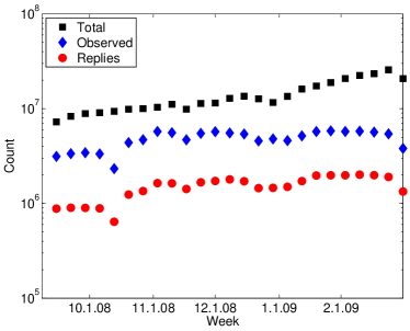
From September 2008 to February 2009, we retrieved over 100 million tweets from the Twitter streaming API service. While the volume of our feed from the Twitter API increased during this study period, the total number of tweets grew at a faster rate (Fig. 2). During this time period, we estimate that we collected roughly 38% of all tweets. The number of messages and percent of which were replies are reported in Table AA4. For the remainder of this paper, we restrict our attention to the nearly 40 million message-reply pairs within this data set and the users who authored these tweets.

Figure 2: Tweet counts are plotted for the weeks between September 2008 and February 2009. The three curves represent the total, those that we observed and the number of the observed tweets that constituted replies.

The data received from the Twitter API service for each tweet contained separate fields for the identification number of the message (message id), the identification number of the user who authored the tweet (user id), the 140 character tweet, and several other geo-spatial and user-specific metadata. If the tweet was made using Twitter’s built-in reply function, the identification number of the message being replied to (original message id) and the identification of the user being replied to (original user id) were also reported.

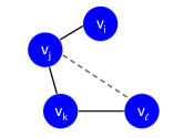
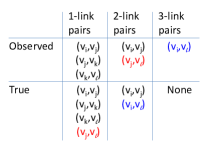
We acknowledge two sources of missing data. First, the Twitter API did not allow us access to all tweets posted during the 6 month period under consideration. Thus, there are replies that we have not observed. As a result, some users may remain unconnected or connected by a path of longer length due to missing intermediary links in our reciprocal-reply network (Fig. 3). Secondly, we acknowledge that users may be interacting with each other and not using the built-in reply function. We discuss this further in the next section.

Figure 3: The effect of missing links in the reciprocal reply network is depicted where observed links are shown as a solid line and an unobserved link is shown as a dashed line. The effect of unobserved links is twofold: (1) some connections between nodes are missed (e.g., $v_{j}$ and $v_{\ell}$ are not connected in the observed reciprocal reply network); and (2) some path lengths between nodes are artificially inflated (e.g., the distance from $v_{i}$ to $v_{\ell}$ is 3 in the observed reciprocal-reply network, however in reality the path length is 2).

2.2 Reciprocal-reply network

In keeping with terminology used in the field of complex networks, the terms nodes and links will be used henceforth to describe users and their connections. Define $\mathcal{G}=(V,E)$ to be a simple graph which contains, $N=|V|$ nodes and $M=|E|$ links. We construct the reciprocal-reply networks in which users are represented by nodes, $v_{i}\in V$, and links connecting two nodes, $e_{ij}\in E$, indicate that $v_{i}$ and $v_{j}$ have made replies to each other during the period of time under analysis (Fig. 1). For each network, we remove self-loops (i.e., users who responded to themselves). We characterize the reciprocal-reply network for each week by the calculation of network statistics such as $N$ (the number of nodes), $\left\langle k\right\rangle$ (average degree), $k_{\max}$ (maximum degree), the number of connected components and $S$ (proportion of nodes in the giant component). We calculate clustering, $C_{G}$, according to Newman’s global clustering coefficient [36]:

$$C_{G}=\frac{3\times(\text{number of triangles on a graph})}{\text{number of connected triples of nodes}}.$$

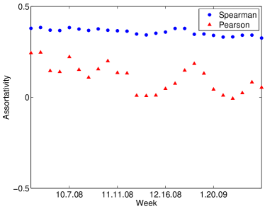
Assortativity refers to the extent to which similar nodes are connected in a network. Often, degree assortativity is quantified by computing the Pearson correlation coefficient of the degrees at each end of links in the network [37]. Since we are interested in quantifying the extent to which the highest degree nodes are connected to other high degree nodes, as defined by the rank of their degrees, we instead measure degree assortativity by the Spearman correlation coefficient. Thus for each link that connects nodes $v_{i}$ and $v_{j}$, we examine the ranks of $k_{v_{i}}$ and $k_{v_{j}}$. The Spearman correlation coefficient, which is the Pearson correlation coefficient applied to the ranks of the degrees at each end of links in the network, is a non-parametric test that does not rely on normally distributed data and is much less sensitive to outliers.

In addition, we also investigate user pairs which are connected by a minimal path length of two (or three) in the reciprocal reply networks. We define $d(v_{i},v_{j})$ to be the path length (i.e., number of links) between nodes $v_{i}$ and $v_{j}$ such that no shorter path exists. As a consequence of missing messages, we recognize that some users will appear to remain unconnected or connected by a path of longer length. Figure 3 depicts the effect of missing links on inferred path lengths between nodes in the network. Nodes $v_{j}$ and $v_{\ell}$ are adjacent in the network, however, due to the missing link represented by the dashed line, these nodes are inferred to be two links apart.

Figure 4: The happiness scores of words are plotted as a function of their rank (dots), with the stop words (words within $\pm\Delta h=1$ of $h_{\text{avg}}=5)$ depicted in light grey [38]. These words were excluded from the happiness score computation. The frequency of words and their rank (1=most frequent, 9956=least frequent) are plotted (solid curve). Not all 10,222 labMT words were observed during the time period from September 2008-February 2009.

Figure 5: A visualization of the 162,445 nodes in the reciprocal reply network for the week beginning December 9, 2008 (Week 14) is depicted. Node colors represent connected components, a total of 15342, with the giant component (shown in blue) comprising 76 % of all nodes. The size of each node is proportional to its degree. The visualization was made using Gephi [39].

Figure 6: Network statistics for the reciprocal-reply network are constructed at the scale of days (green), weeks (blue), and months (red). (A.) The number of users ($N$) engaged in reciprocal exchanges when viewed at the level of days, weeks, or months increases over the study period. (B.) The average degree ($\left\langle k\right\rangle$) remains fairly constant throughout the study period, with higher values detected for larger interaction time periods. (C.) The maximum degree ($k_{\max}$) shows variability throughout the study period. (D.) Clustering decreases quite likely resulting from the inability of the networks’ closed triangles to keep up with the growing number of nodes. (E.) Degree assortativity remains fairly constant throughout the study period, and shows little sensitivity to the time period over which the networks represent interactions. (E.) The proportion of nodes in the giant component ($S$) remains fairly constant for week and month networks, however, shows some variability during the first month of the study for day networks.

2.3 Measuring happiness

To quantify happiness for Twitter users, we apply the real-time hedonometer methodology for measuring sentiment in large-scale text developed in Dodds et al. [11]. In this study, the 5000 most frequently used words from Twitter, Google Books (English), music lyrics (1960 to 2007) and the New York Times (1987 to 2007) were compiled and merged into one list of 10,222 unique words. This word list was chosen solely on the basis of frequency of usage and is independent of any other presupposed significance of individual words. Human subjects scored these 10,222 words on an integer scale from 1 to 9 (1 representing sad and 9 representing happy) using Mechanical Turk. We compute the average happiness score ($h_{\text{avg}}$) to be the average score from 50 independent evaluations. Examples of such words and their happiness scores are: $h_{\text{avg}}$(love)=8.42, $h_{\text{avg}}$(special)=7.20, $h_{\text{avg}}$(house)=6.34, $h_{\text{avg}}$(work)=5.24, $h_{\text{avg}}$(sigh)=4.16, $h_{\text{avg}}$(never)=3.34, $h_{\text{avg}}$(sad)=2.38, $h_{\text{avg}}$(die)=1.74. Words that lie within $\pm\Delta h_{\text{avg}}=1$ of $h_{\text{avg}}$=5 were defined as “stop words” and excluded to sharpen the hedonometer’s resolution. The result is a list of 3,686 words, hereafter referred to as the Language Assessment by Mechanical Turk (labMT) word list [11]. See Tables A1 and A2 for additional example word happiness scores.

$w_{i}$	$h_{\text{avg}}(w_{i})$	labMT?	$f_{i}$	$p_{i}$
Vacation	7.92	yes	1	$\frac{1}{2}$
starts	5.96	yes	n/a	n/a
today	6.22	yes	1	$\frac{1}{2}$
yeahhhhh	n/a	no	n/a	n/a

Table 1: Happiness scores are computed as a weighted average of words’ $h_{\text{avg}}$ scores. Since “starts” is a stop word, it is not included in the calculation of $h_{\text{avg}}(T)=7.07$. This example serves is included as a means to illustrate the methodology; in practice, the average is calculated over a much larger word set.

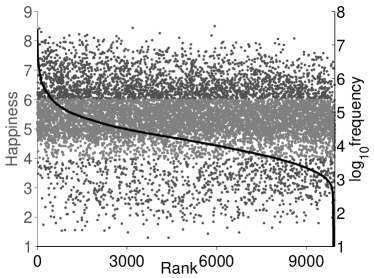
Figure 4 presents word happiness as a function of usage rank for the roughly 10,000 words in the labMT data set. This figure reveals a frequency independent bias towards the usage of positive words (see [37] for further discussion of this positivity bias). Proceeding with the labMT word list, a pattern-matching script evaluated each tweet for the frequency of words. We compute the happiness of each user by applying the hedonometer to the collection of words from all tweets authored by the user during the given time period. Note that each users’ collection of words likely reflects messages that were not replies. The happiness of this collection of words is taken to be the frequency weighted average of happiness scores for each labMT word as $h_{\text{avg}}(T)=\frac{\sum^{N}_{i=1}h_{\text{avg}}(w_{i})f_{i}}{\sum^{N}_{i=1}f_{i}}=\sum^{N}_{i=1}h_{\text{avg}}(w_{i})p_{i},$ where $h_{\text{avg}}(w_{i})$ is the average happiness of the $i$th word appearing with frequency $f_{i}$ and where $p_{i}$ is the normalized frequency ($p_{i}=\frac{f_{i}}{\sum^{N}_{j=1}f_{j}}$). As a simple example example, we consider the phrase: Vacation starts today, yeahhhhh! in Table 1. In practice, though, the hedonometer is applied to a much larger word set and is not applied to single sentences.

Having found happiness scores for each node (user), we then form happiness-happiness pairs $(h_{v_{i}},h_{v_{j}})$, where $h_{v_{i}}$ and $h_{v_{j}}$ denote the happiness of nodes $v_{i}$ and $v_{j}$ connected by an edge. The Spearman correlation coefficient of these happiness-happiness pairs measures how similar individuals’ average happiness is to that of their nearest neighbors’. Lastly, we investigate the strength of the correlation between users’ average happiness scores and those of other users in the two and three link neighborhoods.

3 Results

3.1 Reciprocal-reply network statistics

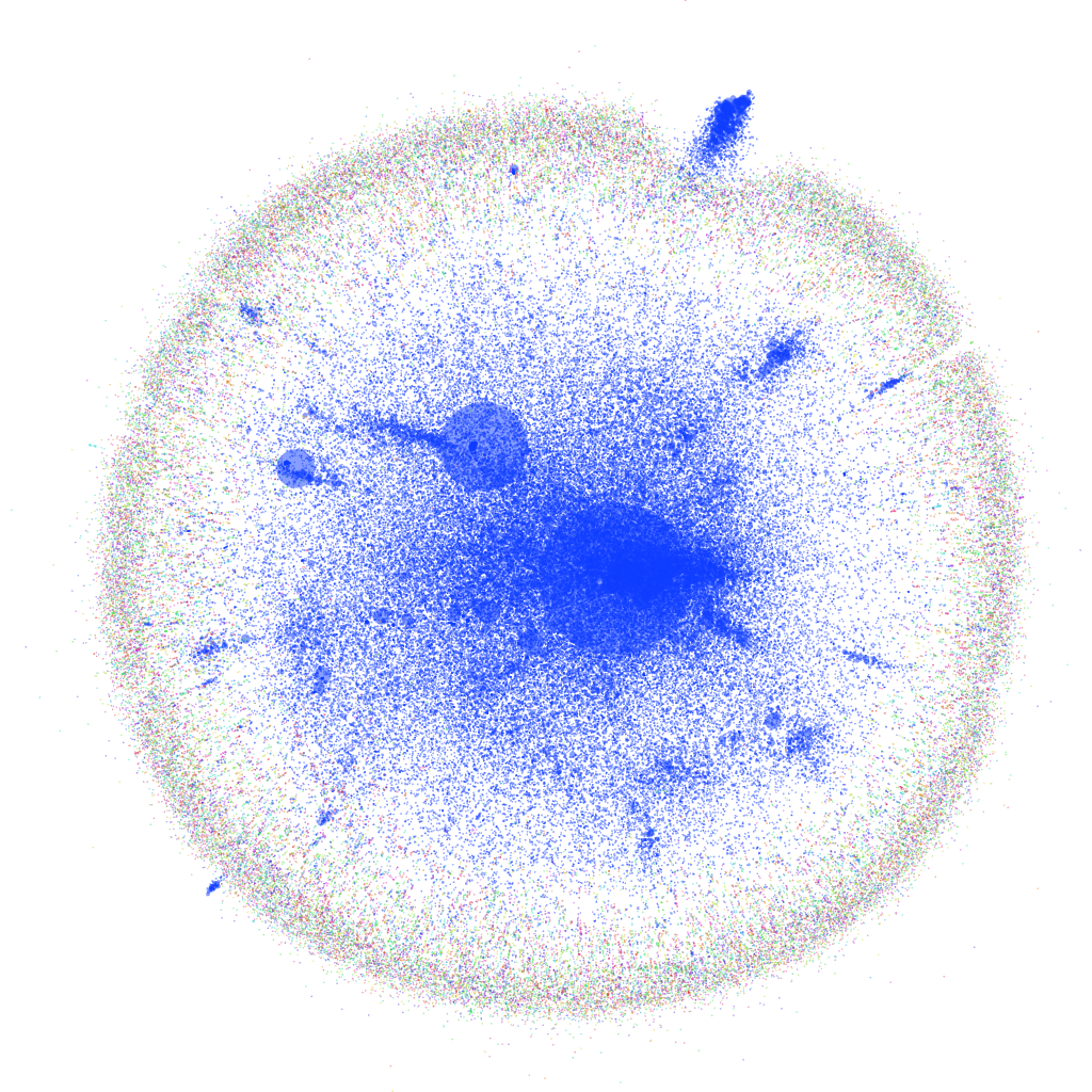
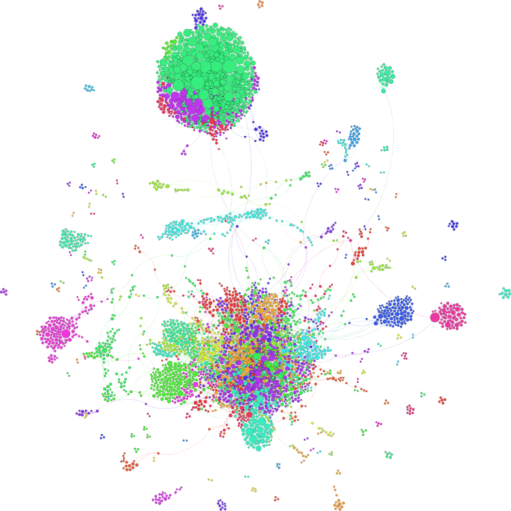
Visualizations of day and week networks were created using the software package Gephi [39]. Figures 5 and A6 show a sample week and day network, respectively. All layouts were produced using the Force Atlas 2 algorithm, which is a spring based algorithm that plots nodes together if they are highly connected (see [40] for more details). The sizes of the nodes are proportional to the degrees.

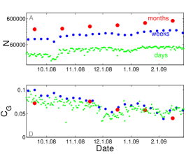
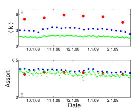
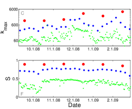
Network statistics, such as the number of nodes (N), the average degree $\left\langle k\right\rangle$, the maximum degree ($k_{\max}$), global clustering $C_{G}$, degree assortativity ($Assort$), and the proportion of nodes in the giant component ($S$) are summarized in Figure 6. Several trends are apparent.

Figure 7: Log-log plot of the complementary cumulative distribution function (CCDF) of the degree distribution for a sample week (week of January 27, 2009) network is shown (blue), along with the best fitting power law model ($\alpha=3.50$ and $k_{\min}=34$) using the procedure of Clauset, Shalizi, and Newman [41]. We test whether the empirical distribution is distinguishable from a power law using the Kolmogorov-Smirnov test and find no evidence against the null hypothesis ($D=2.28\times 10^{-2},p=0.095,n=203852$).

Throughout the course of the study, the number of users in the observed reciprocal-reply network shows an increase, whereas the average degree, degree assortativity, and proportion of nodes in the giant component remain fairly constant. The fluctuations in maximum degree are the result of celebrities or companies having bursts of high volume reply exchanges with their fans during a particular week, for example Bob Bryar, Drummer for the band My Chemical Romance ($k_{\max}=1244$, Week 12), Namecheap domain registration company ($k_{\max}=1245$, Week 13), Twitter’s own Shorty Awards ($k_{\max}=1456$, Week 14), and Stephen Fry, actor and mega-blogger ($k_{\max}=1718$, Week 22). This observation highlights the importance of examining network data on the appropriate time scale, otherwise information about these kinds of dynamics would be be lost. The clustering coefficient shows a slight decrease over the course of this period. This is most likely due to an increasing number of nodes, which results in a smaller proportion of closed triangles in the network.

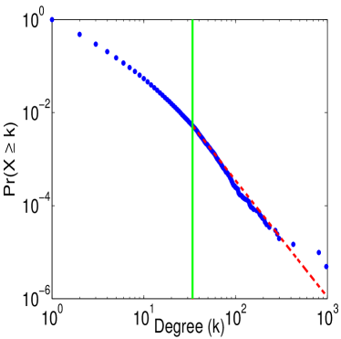
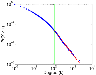
The degree distribution, $P_{k}$, for a sample week (week beginning January 27, 2009) is presented in Figure 7. Using the approach outlined by Clauset, Shalizi, and Newman [41], we find a lower bound for the scaling region to be $k_{\min}\approx 34$ and a very steep scaling exponent of $\alpha=3.5$. This suggests a contrained variance and mean. We test whether the empirical distribution is distinguishable from a power law using the Kolmogorov-Smirnov test and find no evidence against the null hypothesis for the week ($D=2.28\times 10^{-2},p=0.095,n=203852$). We find the same exponent and statistically stronger evidence of a power law for a sample month (see the Appendix, Fig. A1). This suggests that these distributions’ tails may be fit by a power law.

3.2 Measuring happiness

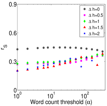
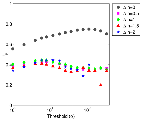
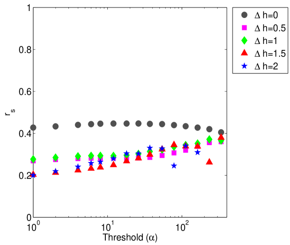
The application of the hedonometer gives reasonable results when applied to a large body of text, but can be misleading when applied to smaller units of language [11]. To provide a sense of how sensitive this measure is to the number of labMT words posted by users, we sampled happiness-happiness pairs, $(h_{v_{i}},h_{v_{j}})$ whose respective users, $v_{i}$ and $v_{j}$, had posted at least $\alpha$ total labMT words during a sample week (week beginning January 27, 2009). For these users, we compute happiness assortativity and show the variation with $\alpha$ in Figure 8. For $\Delta h=0$, there is less variation due to the numerous words centered around the mean happiness score regardless of the threshold, $\alpha$. Tuning both parameters too high results in few sampled words and corrupts the interpretation of the results.

Figure 8: Nearest neighbor happiness assortativity as a function of the number of labMT words required per user is displayed for a sample week reciprocal-reply network. Notice that when $\Delta h=0$, there is less variation due to the numerous words centered around the mean happiness score regardless of the threshold, $\alpha$. While this stability is desirable, tuning $\Delta h$ allows us to sharpen the resolution of the hedonometer. This tuning, however, must be balanced with the appropriate choice of $\alpha$.

Figure 9: Average assortativity of happiness for week networks measured by Spearman’s correlation coefficients as $\Delta h$ is dialed from 0 to 2.5, with $\alpha=50$. As $\Delta h$ increases, the average correlation decreases. For large $\Delta h$ the resulting words under analysis have more disparate happiness scores and thus the correlations between users’ happiness scores are smaller. Similarly, choosing $\Delta h$ to be too small (e.g., $\Delta h=0$) could result in an over estimate of happiness-happiness correlations because of the uni-modal distribution of $h_{\text{avg}}$ for the labMT words. Thus a moderate value for $\Delta h$ is chosen ($\Delta h$ is set to 1 for this study).

(a) $\Delta h=1$, $\alpha=1$

(b) $\Delta h=1$, $\alpha=50$

Figure 10: Happiness assortativity as measured by Spearman’s correlation coefficients is shown for week networks, with $\Delta h=1$ and (a) the threshold of labMT words written by users set to $\alpha=1$ and (b) $\alpha=50$. The dashed lines indicate weakening happiness-happiness correlations as the path length increases from one, two, and three links away, for each week in the data set.

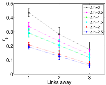
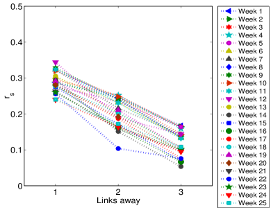
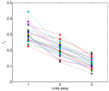
Figures 9 and 10 reveal a weakening happiness-happiness correlation for users in the week networks as the path length between nodes increases. All correlations, for each week, were significant ($p<10^{-10}$). This suggests that the network is assortative with respect to happiness and that user happiness is more similar to their nearest neighbors than those who are 2 or 3 links away.

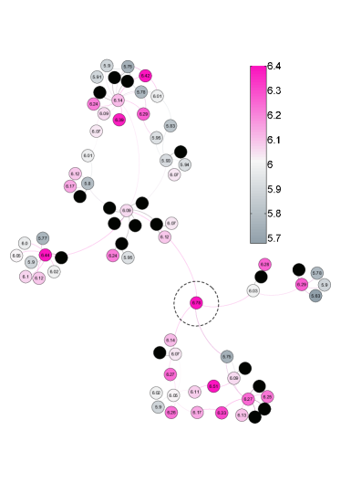
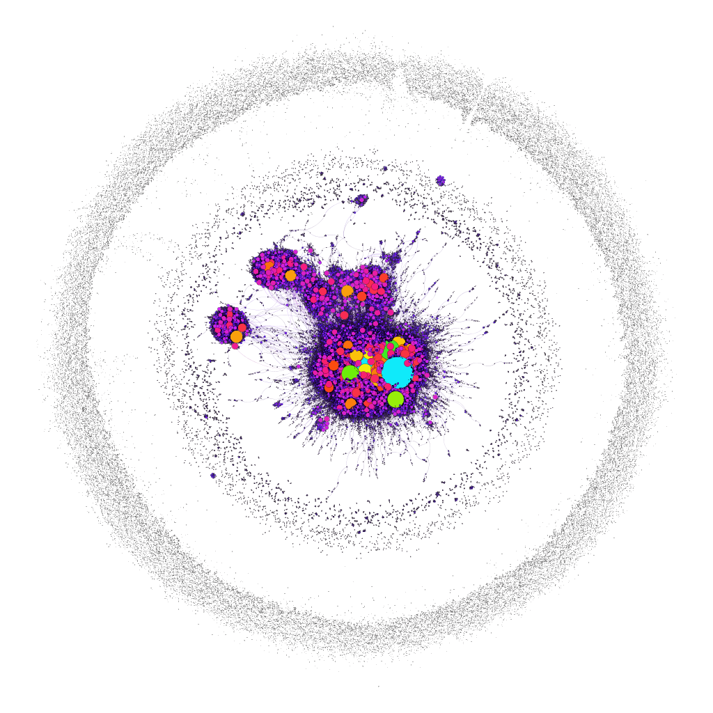
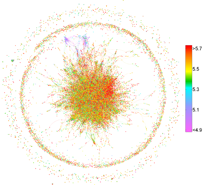
In Figure 11 we provide a visualization of an ego-network for a single node, including neighbors up to three links away. Nodes are colored by their $h_{\text{avg}}$ score, illustrating the assortativity of happiness. Figure A5 visualizes the happiness assortativity for an entire week network.

Figure 11: A visualization of a user and its neighbors 3-links away for a week beginning September 9, 2008 (Week 1). Colors represent happiness scores for users posting more than $\alpha=50$ labMT words. Nodes depicted with the color black are nodes for which the user’s wordbag did not meet our thresholding criteria.

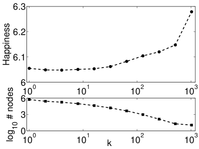
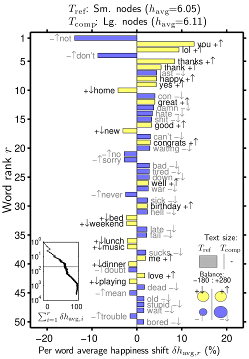
In Figure 12, we show the average happiness score as a function of user degree $k$ for all week networks. The average happiness score increases gradually as a function of degree, with large degree nodes demonstrating a larger average happiness than small degree nodes. Large degree nodes use words such as “you,” “thanks,” and “lol” more frequently than small degree nodes, while the latter group uses words such as “damn,” “hate,” and “tired” more frequently. A word shift diagram, comparing nodes with $k<100$ vs. nodes with $k\geq 100$ is included in the Appendix (Fig. A7). Figure 12 also reveals that the number of large degree nodes is fairly small. Our results support recent work showing that most users of Twitter exhibit an upper limit on the number of active interactions in which they can be engaged [31]. This may provide further evidence in support of Dunbar’s hypothesis, which suggests that the number of meaningful interactions one can have is near 150 [42].

Figure 12: Top Panel: The average happiness score as a function of user degree $k$ for week networks is increasing, as larger degree nodes use fewer negative words (see Figure A7). Bottom Panel: The number of unique users is reported with respect to degree $k$; some users appear in more than one bin because they exhibit different degree $k$ for different weeks of the study.

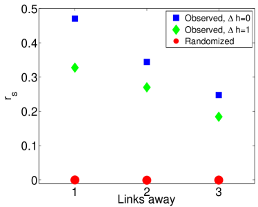
3.3 Testing assortativity against a null model

To further examine these findings, we create a null model which maintains the network topology (i.e., adjacency matrices for one link, two link, and three link remain intact), but randomly permutes the happiness scores associated with each node. The Spearman correlation coefficient shows no statistically significant relationship for the null model applied to a sample week of the data set. Figure 13 shows the results of 100 random permutations applied to nodes’ associated happiness scores. The Spearman correlation coefficients for the observed data are shown as blue squares ($\Delta h_{\text{avg}}=0$) and green diamonds ($\Delta h_{\text{avg}}=1$). The average and standard deviation of the Spearman correlation coefficient calculated for the 100 randomized happiness scores (null model) are shown as red circles with error bars (the error bars are smaller than the symbol). This data supports the hypothesis that happiness is less assortative as network distance increases.

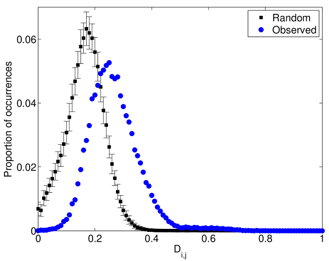
Lastly, we explore whether these correlations are due to similarity of word usage. For this analysis, we compute the similarity of word bags for users connected in the reciprocal reply networks. We compare the distribution of observed similarity scores to similarity scores obtained by randomly reassigning word bags to users. Figure A8 shows that both distributions are of a similar form, with the randomized version exhibiting a slightly lower mean similarity score ($\overline{D_{i,j}}=.167)$ as compared to the mean of the observed similarity scores for users ($\overline{D_{i,j}}=.267)$. If users were tweeting similar words with a similar frequency, we would expect a much larger mean similarity score for the observed data. Thus, we do not find evidence suggesting that the happiness correlations are due to similarity of word bags.

Figure 13: One hundred random permutations were applied to the happiness scores associated with each node in a sample week network (week beginning October 8, 2008 is shown), with $\Delta h=0$ (blue square) and $\Delta h=0$ (green diamonds). The threshold for all cases is set to $\alpha=50$. The Spearman correlation coefficients, $r_{s}$ for the observed data are shown as blue squares. The average and standard deviation of the Spearman correlation coefficient calculated for the 100 randomized data (null model) are shown as red circles with error bars (the error bars are smaller than the symbol). The plot shows Spearman correlation coefficients for the null model to be nearly 0 and provides supporting evidence for our observed trend, namely the network is assortative with respect to happiness and the strength of assortativity decreases as path length increases.

4 Discussion

In this paper, we describe how a social sub-network of Twitter can be derived from reciprocal-replies. Countering claims that Twitter is not social a network [15], we provide evidence of a very social Twitter. The large volume of replies (millions every week) and assortativity of user happiness indicates that Twitter is being used as a social service. Furthermore, conducted at the level of weeks, our analysis examines an in the moment social network, rather than the stale accumulation of social ties over a longer period of time. A network in which edges are created and never disintegrate results in dead links with no contemporary functional activity. This problem of unfriending has been noted [26] and can greatly impact conclusions drawn when observational data are used to infer contagion.

Our characterization of the reciprocal reply network reveals several trends over the 25 week period from September 2008 to February 2009. The number of nodes, $N$, in a given week network increased as time progressed, which is undoubtedly due to Twitter’s enormous growth in popularity over the study period. Similarly, with an increasing number of nodes, we observe a smaller proportion of closed triangles (i.e., clustering shows a slight decrease). This may be due in part to sub-sampling effects or due to an increasing $N$, with which the number of closed triangles (i.e., friends of friends) cannot keep up. The proportion of nodes in the giant component remains fairly constant, as does degree assortativity as measured by Spearman’s correlation coefficient. Had we used the Pearson correlation coefficient, degree assortativity would have been highly variable (Fig. A1) due to the extreme values of maximum degree ($k_{\max}$) during weeks 12-14 and 22. Using the Spearman rank correlation coefficient, which is less sensitive to extreme values, we find that the degree assortativity is fairly constant.

Our work is based on a sub-sample of tweets and is thus subject to the effects of missing data. The problem of missing data has been addressed by several researchers investigating the impact of missing nodes [43, 44, 45, 46, 47], missing links, or both [48]. More specifically, the work of Stumpf [43] shows that sub-sampled scale-free networks are not necessarily themselves scale-free. Further work which addresses the problem of missing messages and identifies the consequences of missing data on inferred network topology is needed to more fully address these questions.

We find support for the “happiness is assortative” hypothesis and evidence that these correlations can be detected up to three links away. Further, this finding does not appear to be based on users tweeting similar words (Fig. A8). Our correlation coefficients for reciprocal-reply networks constructed at the level of weeks are smaller than those obtained by Bollen et al. [8] for a reciprocal-follower network constructed by aggregating over a six month period. This difference is likely a reflection of differences in methodologies, such as our more dynamic time scale (one-week periods vs. six month periods), our exclusion of central value happiness scores (i.e., stop words), and our use of the Spearman correlation coefficient.

While this paper does not attempt to separate homophily and contagion, future work could use reciprocal-reply networks to investigate these effects. While reciprocal-reply networks are subject to errors caused by missing data (see above discussion of this issue) they may provide a valuable framework for studying contagion effects, given that they are based on a conservative and dynamic metric of what constitutes an interaction on Twitter. A network structure in which links are known to be active and valid provides an arena in which the diffusion of information and emotion may be properly studied.

Appendix

Figure A1: Log-log plot of the complementary cumulative distribution function (CCDF) of the degree distribution for a sample month (January 2009) network is shown (blue), along with the best fitting power law model ($\alpha=3.50$ and $k_{\min}=109$) using the procedure of Clauset, Shalizi, and Newman [41]. We test whether the empirical distribution is distinguishable from a power law using the Kolmogorov-Smirnov test and find no evidence against the null hypothesis ($D=1.82\times 10^{-2},p=0.35,n=495881$) data. This distribution may be fit by a power law.

Figure A2: Spearman and Pearson correlation coefficients are used to measure degree assortativity. The Pearson correlation coefficient is more sensitive to extreme values. As a result, the Pearson correlation coefficient obscures the trend that the network is assortative with respect to the rank of node degrees. Given the nature of the degree distribution and the questions that we are asking, we use the Spearman correlation coefficient for our study.

(a) Assortativity of happiness, Pearson’s $r$

(b) Assortativity of happiness, Spearman’s $r$

Figure A3: Measured happiness assortativity as threshold for labMT word usage increases for a single week network. The Spearman correlation coefficient (right) exhibits less variability as compared to the Pearson correlation coefficient (left). Notice that when $\Delta h=0$, there is less variation due to the numerous words centered around the mean happiness score, regardless of the threshold, $\alpha$.

Figure A4: A visualization of the reciprocal reply network for the week beginning September 9, 2008 (Week 1) is depicted. The size of a node is proportional to the degree, and colors further emphasize the degree detected by Gephi s implementation of the algorithm suggested by Blondel et al. [40].

Figure A5: A visualization of the reciprocal reply network for the week beginning September 9, 2008 (Week 1). Colors represent happiness scores for nodes with greater than $\alpha=50$ labMT words (57% of all nodes in the week). The visualization was produced using Gephi [39]. The algorithm employed by the software clusters nodes according to their connectivity. Collections of nodes with similar colors provide a visualization of the happiness is assortativity finding.

Figure A6: A visualization of the reciprocal reply network for the day of October 28, 2008. The size of the nodes is proportional to the degree and colors indicate communities detected by Gephi’s implementation of the community detection algorithm suggested by [49].

.

Figure A7: The collection of words used by nodes with degree $k\geq 100$ ($T_{\text{comp}}$) is compared to words written by users with degree $k<100$ ($T_{\text{ref}}$). Words “award” and “awards” were excluded because their usage dominated the wordbag of one high degree node (Twitter s ShortyAwards). The word “die” was also excluded to eliminate the possibility of the hedonometer incorrectly being applied to German tweets. We note that removal of these words resulted in a negligible change to all values of $r_{s}$ reported in the paper. The horizontal bars on the right side of the plot represent words which raise the happiness score of $T_{\text{comp}}$. The symbols of $+/-$ and $\uparrow/\downarrow$ combine to convey whether a positive/negative word appears more/less frequently in the $T_{\text{comp}}$ as compared to the $T_{\text{ref}}$. Notice that an increase in the usage of positive words (e.g., “you”), as well as a decrease in the use of a negative word (e.g., “last”) will contribute to $T_{\text{comp}}$ having a higher happiness score. On the left hand side of the word shift plot are words which contribute to lowering the happiness score of $T_{\text{comp}}$. Such examples include an increase in the usage of negative words (e.g., “not”) as well as a decrease in the usage of positive words (e.g., “home”). The magnitude of the bars indicate the relative contribution of each word to these effects. In summary, we see that $T_{\text{comp}}$ has a higher happiness score than does $T_{\text{ref}}$. In the lower right, the relative text sizes are depicted as rectangles proportional to the number of words. The reference text, $T_{\text{ref}}$, has considerably more words in its collection than does $T_{\text{comp}}$. The circle plots depicted the relative amount of positive vs. negative words contained in $T_{\text{ref}}$ and $T_{\text{comp}}$. While both collections are similar in terms of positive word usage, the collection of words used by larger nodes contains fewer negative words and thus, this contributes to the slightly higher happiness score for this collection of words. The lower left inset shows the cumulative sum of individual word contributions as a function of $\log_{10}r$, where $r$ is the rank of the 3,686 labMT words. See [11] for the full details of the wordshift graph.

Figure A8: The similarity of word bags for pairs of users connected in a week reciprocal reply network is computed as follows: For users $i$ and $j$, we compute $D_{i,j}=1-\frac{1}{2}\sum^{3686}_{n=1}|f_{i,n}-f_{j,n}|$, where $f_{i,n}$ represents the normalized frequency of word usage of the $n$th labMT word by user $i$. The value of $D_{i,j}$ ranges from 0 (dissimilar word bags) to 1 (similar word bags). The proportion of occurrences of user-user pairs in the reciprocal reply network for a sample week (Sept. 16, 2008) having word similarity indices between 0 and 1 are shown (blue dots), with $\alpha=50$ and $\Delta h=1$. The majority of user-user similarity indices are less than 0.4, indicating that users and their nearest neighbors use dissimilar collections of words in their tweets. We then perform 100 random permutations of word vector assignments to users, while holding the network topology intact (black squares). The resulting distributions show that while users are using more similar words than would be expected by chance, this shift is small. The mean score for randomized user-user paired word collections is $\overline{D_{i,j}}=.167$. This value is not zero, since users are using a common language (English). The mean score for our observed network data is $\overline{D_{i,j}}=.267$, which is slightly higher than the randomized value due to conversations occurring between these users.

Rank	Word	Frequency	Happiness		Rank	Word	Frequency	Happiness		Rank	Word	Frequency	Happiness
		$(\times 10^{5})$					$(\times 10^{5})$					$(\times 10^{5})$
1	you	103.55	6.24		51	sure	6.82	6.32		101	music	4.24	8.02
2	my	94.91	6.16		52	done	6.81	6.54		102	found	4.23	6.54
3	me	56.35	6.58		53	show	6.73	6.24		103	doesn’t	4.23	3.62
4	not	39.98	3.86		54	awesome	6.72	7.60		104	online	4.23	6.72
5	up	36.04	6.14		55	check	6.51	6.10		105	party	4.20	7.58
6	no	34.40	3.48		56	bed	6.42	7.18		106	soon	4.20	6.34
7	new	34.03	6.82		57	sleep	6.33	7.16		107	thinking	4.15	6.28
8	like	31.75	7.22		58	cool	6.32	7.20		108	snow	4.14	6.32
9	all	30.71	6.22		59	live	6.29	6.84		109	give	4.13	6.54
10	good	30.20	7.20		60	big	6.28	6.22		110	movie	4.12	6.84
11	will	23.58	6.02		61	free	6.18	7.96		111	ha	4.09	6.00
12	we	22.59	6.38		62	life	6.17	7.32		112	sorry	4.08	3.66
13	day	21.80	6.24		63	old	6.07	3.98		113	real	4.06	6.78
14	know	19.45	6.10		64	didn’t	6.04	4.00		114	kids	3.98	7.38
15	more	19.32	6.24		65	find	6.00	6.00		115	phone	3.91	6.44
16	don’t	18.29	3.70		66	die	6.00	1.74		116	tv	3.91	6.70
17	today	18.24	6.22		67	video	5.99	6.48		117	stop	3.89	3.90
18	love	17.66	8.42		68	house	5.99	6.34		118	play	3.88	7.26
19	think	17.45	6.20		69	christmas	5.89	7.96		119	waiting	3.88	3.68
20	see	15.28	6.06		70	playing	5.77	7.14		120	lunch	3.81	7.42
21	great	14.60	7.88		71	world	5.76	6.52		121	food	3.79	7.44
22	lol	13.35	6.84		72	game	5.54	6.92		122	reading	3.76	6.78
23	thanks	13.09	7.40		73	wow	5.54	7.46		123	god	3.74	7.28
24	home	13.05	7.14		74	ready	5.53	6.58		124	top	3.65	6.76
25	people	12.71	6.16		75	iphone	5.53	6.54		125	buy	3.60	6.28
26	night	12.70	6.22		76	listening	5.41	6.28		126	book	3.56	7.24
27	blog	12.26	6.02		77	pretty	5.40	7.32		127	car	3.56	6.72
28	last	11.89	3.74		78	always	5.39	6.48		128	idea	3.52	7.06
29	well	11.70	6.68		79	help	5.27	6.08		129	friend	3.51	7.66
30	make	11.27	6.00		80	read	5.07	6.52		130	family	3.51	7.72
31	right	11.04	6.54		81	google	5.05	7.20		131	yay	3.47	6.10
32	can’t	10.93	3.42		82	everyone	5.03	6.12		132	glad	3.47	7.48
33	morning	10.38	6.56		83	most	4.95	6.22		133	least	3.46	4.00
34	very	10.10	6.12		84	wait	4.88	3.74		134	nothing	3.44	3.90
35	first	9.69	6.82		85	start	4.87	6.10		135	late	3.43	3.46
36	our	9.26	6.08		86	please	4.79	6.36		136	internet	3.39	7.48
37	better	8.89	7.00		87	con	4.78	3.70		137	amazing	3.38	7.66
38	us	8.82	6.26		88	try	4.77	6.02		138	mean	3.38	3.68
39	tonight	8.79	6.14		89	thought	4.69	6.38		139	myself	3.37	6.30
40	down	8.73	3.66		90	school	4.66	6.26		140	facebook	3.34	6.08
41	happy	8.40	8.30		91	thank	4.64	7.40		141	funny	3.32	7.92
42	tomorrow	7.88	6.18		92	weekend	4.56	8.00		142	tired	3.29	3.34
43	nice	7.80	7.38		93	hey	4.48	6.06		143	talk	3.29	6.06
44	best	7.61	7.18		94	wish	4.44	6.92		144	damn	3.26	2.98
45	she	7.57	6.18		95	hate	4.42	2.34		145	interesting	3.26	7.52
46	yes	7.42	6.74		96	haha	4.41	7.64		146	own	3.24	6.16
47	fun	7.37	7.96		97	friends	4.41	7.92		147	friday	3.23	6.88
48	hope	7.34	7.38		98	making	4.40	6.24		148	open	3.18	6.10
49	bad	6.98	2.64		99	dinner	4.27	7.40		149	lost	3.16	2.76
50	never	6.92	3.34		100	coffee	4.27	7.18		150	guys	3.16	6.22

Table A1: The top 150 most frequently occurring words from the labMT list in our Sept 2008 through Feb 2009 data set, where stop words ($4<h_{\text{avg}}<6$) have been removed.

Rank	Word	Frequency	Happiness		Rank	Word	Frequency	Happiness		Rank	Word	Frequency	Happiness
		$(\times 10^{5})$					$(\times 10^{5})$					$(\times 10^{5})$
1	the	295.60	4.98		51	an	22.73	4.84		101	el	11.76	4.80
2	to	249.91	4.98		52	we	22.59	6.38		102	well	11.70	6.68
3	i	221.28	5.92		53	some	22.32	5.02		103	oh	11.69	4.84
4	a	218.13	5.24		54	que	22.26	4.64		104	who	11.64	5.06
5	and	135.23	5.22		55	day	21.80	6.24		105	should	11.48	5.24
6	is	127.94	5.18		56	how	21.64	4.68		106	over	11.34	4.82
7	in	122.94	5.50		57	going	20.64	5.42		107	make	11.27	6.00
8	of	121.79	4.94		58	am	20.60	5.38		108	then	11.15	5.34
9	for	114.41	5.22		59	go	20.03	5.54		109	right	11.04	6.54
10	you	103.55	6.24		60	has	19.68	5.18		110	can’t	10.93	3.42
11	on	96.97	5.56		61	or	19.55	4.98		111	way	10.84	5.24
12	my	94.91	6.16		62	know	19.45	6.10		112	only	10.72	4.92
13	it	91.09	5.02		63	more	19.32	6.24		113	getting	10.63	5.68
14	that	69.81	4.94		64	la	18.77	5.00		114	his	10.56	5.56
15	at	58.51	4.90		65	don’t	18.29	3.70		115	morning	10.38	6.56
16	with	56.42	5.72		66	today	18.24	6.22		116	very	10.10	6.12
17	me	56.35	6.58		67	too	18.15	5.22		117	after	9.82	5.08
18	just	50.25	5.76		68	they	18.09	5.62		118	watching	9.76	5.84
19	have	49.86	5.82		69	work	17.95	5.24		119	her	9.73	5.84
20	be	46.10	5.68		70	got	17.91	5.60		120	them	9.71	4.92
21	this	45.75	5.06		71	love	17.66	8.42		121	first	9.69	6.82
22	de	44.38	4.82		72	think	17.45	6.20		122	e	9.66	4.72
23	so	40.93	5.08		73	back	17.37	5.18		123	that’s	9.55	5.28
24	not	39.98	3.86		74	twitter	17.18	5.46		124	rt	9.52	4.88
25	i’m	39.89	5.74		75	when	16.84	4.96		125	y	9.47	4.48
26	are	39.03	5.16		76	there	16.39	5.10		126	than	9.42	4.74
27	but	37.78	4.24		77	had	15.30	4.74		127	its	9.36	4.96
28	was	37.74	4.60		78	see	15.28	6.06		128	our	9.26	6.08
29	up	36.04	6.14		79	en	14.97	4.84		129	better	8.89	7.00
30	out	35.20	4.62		80	really	14.93	5.84		130	us	8.82	6.26
31	now	35.12	5.90		81	off	14.89	4.02		131	tonight	8.79	6.14
32	no	34.40	3.48		82	great	14.60	7.88		132	down	8.73	3.66
33	new	34.03	6.82		83	need	14.45	4.84		133	i’ve	8.59	5.58
34	do	33.96	5.76		84	he	14.34	5.42		134	u	8.40	5.52
35	from	33.78	5.18		85	still	13.74	5.14		135	happy	8.40	8.30
36	like	31.75	7.22		86	been	13.43	5.04		136	again	8.34	5.42
37	your	31.43	5.60		87	lol	13.35	6.84		137	could	8.34	5.52
38	all	30.71	6.22		88	would	13.15	5.38		138	un	8.15	4.64
39	good	30.20	7.20		89	thanks	13.09	7.40		139	into	8.08	5.04
40	get	30.04	5.92		90	home	13.05	7.14		140	i’ll	8.05	5.38
41	what	29.46	4.80		91	want	12.81	5.70		141	man	7.99	5.90
42	about	28.97	5.16		92	people	12.71	6.16		142	tomorrow	7.88	6.18
43	it’s	27.14	4.88		93	night	12.70	6.22		143	nice	7.80	7.38
44	if	25.21	4.66		94	here	12.28	5.48		144	any	7.70	5.22
45	by	24.66	4.98		95	o	12.26	4.96		145	take	7.63	5.18
46	as	24.50	5.22		96	blog	12.26	6.02		146	best	7.61	7.18
47	time	24.19	5.74		97	why	12.10	4.98		147	she	7.57	6.18
48	one	23.73	5.40		98	much	11.92	5.74		148	even	7.42	5.58
49	will	23.58	6.02		99	last	11.89	3.74		149	yes	7.42	6.74
50	can	23.57	5.62		100	did	11.84	5.58		150	little	7.38	4.60

Table A2: The top 150 most frequently occurring words from the labMT word list in our Sept 2008 through Feb 2009 data set including stop words.

Week	Start date	$N$	$<k>$	$k_{\max}$	$C_{G}$	Assort	# Comp.	$S$
1	09.09.08	95647	2.99	261	0.10	0.24	10364	0.71
2	09.16.08	99236	2.95	313	0.10	0.24	11062	0.71
3	09.23.08	99694	2.90	369	0.09	0.13	11457	0.70
4	09.30.08	100228	2.87	338	0.09	0.13	11752	0.69
5	10.07.08	78296	2.60	241	0.09	0.21	11140	0.63
6	10.14.08	122644	3.20	394	0.09	0.14	12221	0.74
7	10.21.08	130027	3.30	559	0.08	0.09	12420	0.75
8	10.28.08	144036	3.56	492	0.08	0.14	12319	0.78
9	11.04.08	145346	3.54	330	0.08	0.19	12597	0.78
10	11.11.08	136534	3.35	441	0.08	0.12	12972	0.76
11	11.18.08	153486	3.46	444	0.08	0.13	13594	0.77
12	11.25.08	155753	3.46	1244	0.06	0.00	14122	0.77
13	12.02.08	165156	3.44	1245	0.06	0.01	14496	0.78
14	12.09.08	162445	3.33	1456	0.05	0.01	15342	0.76
15	12.16.08	148154	3.12	730	0.06	0.04	15645	0.73
16	12.23.08	140871	3.22	575	0.07	0.07	15216	0.72
17	12.30.08	143015	3.30	519	0.07	0.15	15272	0.73
18	01.06.09	170597	3.19	253	0.07	0.18	17234	0.74
19	01.13.09	188429	3.29	477	0.07	0.13	18403	0.75
20	01.20.09	196038	3.16	680	0.06	0.04	19927	0.74
21	01.27.09	203852	3.04	973	0.05	0.01	21537	0.73
22	02.03.09	212513	2.92	1718	0.04	-0.01	24387	0.71
23	02.10.09	213936	2.83	828	0.06	0.02	25854	0.70
24	02.17.09	215172	2.65	437	0.06	0.07	28742	0.67
25	02.24.09	170180	2.27	320	0.06	0.04	28388	0.58

Table A3: Network statistics for reciprocal-reply networks by week. As Twitter popularity grows, so does the number of users ($N$) in the observed reciprocal-reply network. The average degree ($<k>$), degree assortativity, the number of nodes in the giant component (# Comp.), and the proportion of nodes in the giant component ($S$) remain fairly constant, whereas the maximum degree ($k_{\max}$) shows a great deal of variability from month to month. Clustering ($C_{G}$) shows a slight decrease over the course of this period.

Week	Start date	# Obsvd. Msgs.	# Total Msgs.	% Obsvd.	# Replies	% Replies
		$\times 10^{6}$	$\times 10^{6}$	$\left(\frac{\#Obsvd.}{\#Total}\times 100\right)$	$\times 10^{6}$	$\left(\frac{\#Replies}{\#Obsvd.}\times 100\right)$
1	09.09.08	3.14	7.26	43.2	0.88	28.1
2	09.16.08	3.36	8.31	40.4	0.90	26.9
3	09.23.08	3.43	8.89	38.6	0.90	26.2
4	09.30.08	3.33	9.06	36.8	0.89	26.6
5	10.07.08	2.33	9.38	24.8	0.64	27.5
6	10.14.08	4.39	9.87	44.4	1.24	28.3
7	10.21.08	4.70	10.01	47.0	1.35	28.8
8	10.28.08	5.74	10.34	55.5	1.64	28.5
9	11.04.08	5.58	11.14	50.1	1.63	29.3
10	11.11.08	4.70	9.88	47.6	1.42	30.2
11	11.18.08	5.48	11.34	48.3	1.67	30.5
12	11.25.08	5.71	11.47	49.8	1.73	30.2
13	12.02.08	5.54	12.85	43.1	1.80	32.4
14	12.09.08	5.41	13.54	39.9	1.72	31.7
15	12.16.08	4.57	12.72	35.9	1.45	31.8
16	12.23.08	4.80	11.62	41.3	1.46	30.5
17	12.30.08	4.61	13.48	34.2	1.50	32.5
18	01.06.09	5.16	16.11	32.0	1.72	33.3
19	01.13.09	5.73	17.33	33.1	1.97	34.4
20	01.20.09	5.82	18.87	30.9	1.98	34.1
21	01.27.09	5.75	20.79	27.6	1.98	34.5
22	02.03.09	5.78	22.42	25.8	2.01	34.8
23	02.10.09	5.66	23.39	24.2	1.99	35.1
24	02.17.09	5.43	25.71	21.1	1.91	35.1
25	02.24.09	3.80	20.75	18.3	1.34	35.1

Table A4: The number of “observed” messages in our database comprise a fraction of the total number of Twitter message made during period of this study (September 2008 through February 2009). While our feed from the Twitter API remains fairly constant, the total # of tweets grows, thus reducing the % of all tweets observed in our database. We calculate the total $\#$ of messages as the difference between the last message id and the first message id that we observe for a given month. This provides a reasonable estimation of the number of tweets made per month as message ids were assigned (by Twitter) sequentially during the time period of this study. We also report the number observed messages that are replies to specific messages and the percentage of our observed messages which constitute replies.

References

- Stanley Wasserman [1994] K. F. Stanley Wasserman, Social network analysis: methods and applications Volume 8 of Structural analysis in the social sciences, Cambridge University Press, Cambridge, 1994.
- Gjoka et al. [2010] M. Gjoka, M. Kurant, C. Butts, A. Markopoulou, Walking in facebook: A case study of unbiased sampling of osns, in: INFOCOM, 2010 Proceedings IEEE, pp. 1 –9.
- Viswanath et al. [2009] B. Viswanath, A. Mislove, M. Cha, K. P. Gummadi, On the evolution of user interaction in facebook, in: Proceedings of the 2nd ACM workshop on Online social networks, WOSN ’09, ACM, New York, NY, USA, 2009, pp. 37–42.
- Papacharissi [2009] Z. Papacharissi, The virtual geographies of social networks: a comparative analysis of facebook, linkedin and asmallworld, New Media & Society 11 (February/March 2009) 199–220.
- Dodds and Danforth [2010] P. Dodds, C. M. Danforth, Measuring the happiness of large-scale written expression: Songs, blogs, and presidents, Journal of Happiness Studies 11 (2010) 441–456. 10.1007/s10902-009-9150-9.
- Java et al. [2009] A. Java, X. Song, T. Finin, B. Tseng, Why we twitter: An analysis of a microblogging community, in: H. Zhang, M. Spiliopoulou, B. Mobasher, C. Giles, A. McCallum, O. Nasraoui, J. Srivastava, J. Yen (Eds.), Advances in Web Mining and Web Usage Analysis, volume 5439 of Lecture Notes in Computer Science, Springer Berlin / Heidelberg, 2009, pp. 118–138.
- Bakshy et al. [2011] E. Bakshy, J. M. Hofman, W. A. Mason, D. J. Watts, Everone’s an influencer: Quantifying influence on twitter, in: WSDM ’11: Proceedings of the fourth ACM international conference on Web search and data mining, ACM, New York, NY, USA, 2011. 618113.
- Bollen et al. [2011a] J. Bollen, B. Goncalves, G. Ruan, H. Mao, Happiness is assortative in online social networks, Artificial Life 17 (2011a).
- Bollen et al. [2011b] J. Bollen, H. Mao, X. Zeng, Twitter mood predicts the stock market, Journal of Computational Science 2 (2011b) 1–8.
- Cha et al. [2010] M. Cha, H. Haddadi, F. Benevenuto, K. P. Gummadi, Measuring user influence in twitter: The million follower fallacy, in: in ICWSM 10: Proceedings of international AAAI Conference on Weblogs and Social.
- Dodds et al. [2011] P. S. Dodds, K. D. Harris, I. M. Kloumann, C. A. Bliss, C. M. Danforth, Temporal patterns of happiness and information in a global social network: Hedonometrics and twitter, PLoS ONE 6 (2011) e26752.
- Guo et al. [2009] L. Guo, E. Tan, S. Chen, X. Zhang, Y. E. Zhao, Analyzing patterns of user content generation in online social networks, in: Proceedings of the 15th ACM SIGKDD international conference on Knowledge discovery and data mining, KDD ’09, ACM, New York, NY, USA, 2009, pp. 369–378.
- Huberman et al. [2008] B. A. Huberman, D. M. Romero, F. Wu, Social networks that matter: Twitter under the microscope, CoRR abs/0812.1045 (2008).
- Kim et al. [2009] E. Kim, S. Gilbert, M. J. Edwards, E. Graeff, Detecting sadness in 140 characters: Sentiment analysis of mourning michael jackson on twitter (2009).
- Kwak et al. [2010] H. Kwak, C. Lee, H. Park, S. Moon, What is twitter, a social network or a news media?, in: Proceedings of the 19th international conference on World wide web, WWW ’10, ACM, New York, NY, USA, 2010, pp. 591–600.
- Thelwall et al. [2011] M. Thelwall, K. Buckley, G. Paltoglou, Sentiment in twitter events, Journal of the American Society for Information Science and Technology 62 (2011) 406–418.
- Weng et al. [2010] J. Weng, E.-P. Lim, J. Jiang, Q. He, Twitterrank: finding topic-sensitive influential twitterers, in: Proceedings of the third ACM international conference on Web search and data mining, WSDM ’10, ACM, New York, NY, USA, 2010, pp. 261–270.
- Tan et al. [2011] C. Tan, L. Lee, J. Tang, L. Jiang, M. Zhou, P. Li, User-level sentiment analysis incorporating social networks, ArXiv e-prints (2011).
- Ugander et al. [2012] J. Ugander, L. Backstrom, C. Marlow, J. Kleinberg, Structural diversity in social contagion, Proceedings of the National Academy of Sciences 109 (2012) 5962–5966.
- Christakis and Fowler [2007] N. A. Christakis, J. H. Fowler, The spread of obesity in a large social network over 32 years, New England Journal of Medicine 357 (2007) 370–379.
- Fowler and Christakis [2008] J. H. Fowler, N. A. Christakis, Dynamic spread of happiness in a large social network: longitudinal analysis over 20 years in the framingham heart study, BMJ 337 (2008).
- Christakis and Fowler [2008] N. A. Christakis, J. H. Fowler, The collective dynamics of smoking in a large social network, New England Journal of Medicine 358 (2008) 2249–2258.
- Rosenquist et al. [2010] J. N. Rosenquist, J. Murabito, J. H. Fowler, N. A. Christakis, The spread of alcohol consumption behavior in a large social network, Annals of Internal Medicine 152 (2010) 426–433.
- Hill et al. [2010] A. L. Hill, D. G. Rand, M. A. Nowak, N. A. Christakis, Emotions as infectious diseases in a large social network: the sisa model, Proceedings of the Royal Society B: Biological Sciences 277 (2010) 3827–3835.
- Christakis and Fowler [2011] N. A. Christakis, J. H. Fowler, Social Contagion Theory: Examining Dynamic Social Networks and Human Behavior, ArXiv e-prints (2011).
- Noel et al. [2011] H. Noel, W. Galuba, B. Nyhan, The unfriending problem: The consequences of homophily in friendship retention for causal estimates of social influence, Social Networks 33 (2011) 211–218.
- Lyons [2011] R. Lyons, The spread of evidence-poor medicine via flawed social-network analysis, Statistics, Politics, and Policy 2 (2011) 1–26.
- Shalizi and Thomas [2011] C. R. Shalizi, A. C. Thomas, Homophily and contagion are generically confounded in observational social network studies, Sociological Methods & Research 40 (2011) 211–239.
- Romero et al. [2011] D. M. Romero, B. Meeder, J. Kleinberg, Differences in the mechanics of information diffusion across topics: Idioms, political hashtags, and complex contagion on Twitter, in: Proceedings of World Wide Web Conference.
- blo [2011] Twitter api blog, 2011. Http://blog.twitter.com/2011/09/one-hundred-million-voices.
- Gon alves et al. [2011] B. Gon alves, N. Perra, A. Vespignani, Modeling users’ activity on twitter networks: Validation of dunbar’s number, PLoS ONE 6 (2011) e22656.
- Watts and Dodds [2007] D. J. Watts, P. S. Dodds, Influentials, networks, and public opinion formation, Journal of Consumer Research 34 (2007) pp. 441–458.
- Grannis [2010] R. Grannis, Six degrees of who cares? , American Journal of Sociology 115 (2010) pp. 991–1017.
- Golder and Macy [2011] S. A. Golder, M. W. Macy, Diurnal and seasonal mood vary with work, sleep, and daylength across diverse cultures, Science Magazine 333 (2011) 1878–1881.
- Miller [2011] G. Miller, Social Scientists wade into the Tweet stream, Science Magazine 333 (2011) 1814–1815.
- Newman [2001] M. Newman, The structure of scientific collaboration networks, Proceedings of the National Academy, USa 98 (2001) 404–409.
- Newman [2002] M. Newman, Assortative mixing in networks, Physical Review Letters 89 (2002) 208701.
- Kloumann et al. [2012] I. M. Kloumann, C. M. Danforth, K. D. Harris, C. A. Bliss, P. S. Dodds, Positivity of the english language, PLoS ONE 7 (2012) e29484.
- Bastian et al. [2009] M. Bastian, S. Heymann, M. Jacomy, Gephi: An open source software for exploring and manipulating networks, 2009.
- Jacomy et al. [2012] M. Jacomy, S. Heymann, T. Venturini, M. Bastian, Forceatlas2, a graph layout algorithm for handy network visualization, http://www.medialab.sciences-po.fr/publications/Jacomy_Heymann_Venturini-Force_Atlas2.pdf, 2012.
- Clauset et al. [2009] A. Clauset, C. R. Shalizi, M. E. J. Newman, Power-law distributions in empirical data, SIAM Review 51 (2009) 661–703.
- Dunbar [1995] R. Dunbar, Neocortex size and group size in primates: a test of the hypothesis, Journal of Human Evolution 28 (1995) 287 – 296.
- Stumpf et al. [2005] M. P. H. Stumpf, C. Wiuf, R. M. May, Subnets of scale-free networks are not scale-free: Sampling properties of networks, Proceedings of the National Academy of Sciences of the United States of America 102 (2005) 4221–4224.
- Sadikov et al. [2011] E. Sadikov, M. Medina, J. Leskovec, H. Garcia-Molina, Correcting for missing data in information cascades, in: Proceedings of the fourth ACM international conference on Web search and data mining, WSDM ’11, ACM, New York, NY, USA, 2011, pp. 55–64.
- Leskovec and Faloutsos [2006] J. Leskovec, C. Faloutsos, Sampling from large graphs, in: Proceedings of the 12th ACM SIGKDD international conference on Knowledge discovery and data mining, KDD ’06, ACM, New York, NY, USA, 2006, pp. 631–636.
- Lee et al. [2006] S. H. Lee, P.-J. Kim, H. Jeong, Statistical properties of sampled networks, Phys. Rev. E 73 (2006) 016102.
- Frantz et al. [2009] T. Frantz, M. Cataldo, K. Carley, Robustness of centrality measures under uncertainty: Examining the role of network topology, Computational & Mathematical Organization Theory 15 (2009) 303–328.
- Kossinets [2006] G. Kossinets, Effects of missing data in social networks, Social Networks 28 (2006) 247–268.
- Blondel et al. [2008] V. D. Blondel, J.-L. Guillaume, R. Lambiotte, E. Lefebvre, Fast unfolding of communities in large networks, Journal of Statistical Mechanics: Theory and Experiment 2008 (2008) P10008.