Debye–Hückel solution for steady electro-osmotic flow of a micropolar fluid in a cylindrical microcapillary

Abuzar A. Siddiqui¹ and Akhlesh Lakhtakia²

¹Department of Basic Sciences, Bahauddin Zakariya University, Multan, Pakistan.

²Nanoengineered Metamaterials Group, Department of Engineering Science and Mechanics, Pennsylvania State University, University Park, PA 16802, USA.

Abstract Analytic expressions for the speed, flux, microrotation, stress, and couple stress in a micropolar fluid exhibiting steady, symmetric and one-dimensional electro-osmotic flow in a uniform cylindrical microcapillary were derived under the constraint of the Debye–Hückel approximation, which is applicable when the cross-sectional radius of the microcapillary exceeds the Debye length, provided that the zeta potential is sufficiently small in magnitude. As the aciculate particles in a micropolar fluid can rotate without translation, micropolarity influences fluid speed, fluid flux, and one of the two non-zero components of the stress tensor. The axial speed in a micropolar fluid intensifies as the radius increases. The stress tensor is confined to the region near the wall of the microcapillary but the couple stress tensor is uniform across the cross-section.

Keywords:couple stress; electro-osmosis; microcapillary; micropolar fluid; microrotation; steady flow

1 Introduction

Electro-osmotic flows on the micrometer scale occur in many technoscientific settings, including: microchannels in chips for protein analysis and intravenous drug delivery [1]; microchannels in biological and chemical instruments [2]; micropumps, microturbines, and micromachines [3, 4, 5]; injectors of detoxification agents [6]; and water desalinators [7]. These flows occur by virtue of the movement of free ions in the liquid in the electric double layer (EDL) when an electric field is applied, and, in turn, cause bulk motion of the entire fluid. The EDL is an infinitesimal region between a layer of charges of one polarity on the electrolytic-liquid side of the solid-liquid interface (i.e., the wall of the channel) and a layer of charges of the opposite polarity on the solid side.

The discovery of electro-osmosis is just about two centuries old [8]. Fifty years after that event, electro-osmotic flow in a channel was experimentally found to be proportional to the applied current, which prompted Helmholtz to develop the EDL theory in 1879. Two decades later, the EDL thickness was measured as much smaller than the cross-sectional dimensions of the channel. In 1923, Debye and Hückel published their analysis on the distribution of ions in a low-ionic-energy solution by using the Boltzmann distribution for the ionic energy [9], a seminal work that is widely used even nowadays.

Many fluids are not simple Newtonian fluids—wherein stress is a symmetric tensor of the second rank. Instead, these fluids are micropolar as they contain aciculate particles that can rotate about axes passing through their centroids [10, 11]. Therefore, not only is stress asymmetric in micropolar fluids but they also sustain body couples.

Micropolar fluids are exemplified by colloidal suspensions, liquid crystals, and epoxies [12]. Blood too is micropolar [13, 14], along with other body fluids containing particulate materials. As body fluids are subjected to electric fields in labs-on-a-chip [15], electro-osmotic flows of micropolar fluids in microchannels [16, 17] are of emerging technoscientific importance in nanomedicine [18, 19].

Our present interest lies in the spatial characteristics of fluid speed, stress, microrotation, and couple stress in a micropolar fluid flowing steadily in a microcapillary of circular cross-section with a cross-sectional radius exceeding the Debye length. With the assumption that zeta potential due to the EDL is sufficiently small, the Debye–Hückel approximation can be applied to obtain analytical results. Analysis of these results would clearly show how the micropolarity influences fluid flow.

This paper is organized as follows: The formulation of the relevant boundary–value problem is presented in Sec. 2, while Sec. 3 contains the description of analytical solution of the problem based on the Debye–Hückel approximation. Section 4 contains numerical illustrations of the obtained analytical results and discussions thereon. The main conclusions are summarized in Sec. 5.

2 Basic Analysis

In a micropolar fluid, the stress tensor $\underline{\underline{\sigma}}^{\prime}$ is defined as a function of position ${\bf r}^{\prime}$ as

$$\underline{\underline{\sigma}}^{\prime}({\bf r}^{\prime})=-p^{\prime}({\bf r}^{\prime})\underline{\underline{I}}+\lambda\underline{\underline{I}}\nabla^{\prime}\mbox{ \tiny{${}^{\bullet}$} }{\bf V}^{\prime}({\bf r}^{\prime})+(\mu+\chi/2)\left\{\nabla^{\prime}{\bf V}^{\prime}({\bf r}^{\prime})+\left[\nabla^{\prime}{\bf V}^{\prime}({\bf r}^{\prime})\right]^{T}\right\}$$

$$\qquad\qquad-(\chi/2)\underline{\underline{I}}\times\left[\nabla^{\prime}\times{\bf V}^{\prime}({\bf r}^{\prime})\right]+\chi\underline{\underline{I}}\times{\bf v}^{\prime}({\bf r}^{\prime})\,,$$ (1)

and the couple stress tensor $\underline{\underline{m}}^{\prime}$ as

$$\underline{\underline{m}}^{\prime}({\bf r}^{\prime})=\alpha\underline{\underline{I}}\nabla^{\prime}\mbox{ \tiny{${}^{\bullet}$} }{\bf v}^{\prime}({\bf r}^{\prime})+\beta\nabla^{\prime}{\bf v}^{\prime}({\bf r}^{\prime})+\gamma\left[\nabla^{\prime}{\bf v}^{\prime}({\bf r}^{\prime})\right]^{T}\,.$$ (2)

Here, $\underline{\underline{I}}=\nabla^{\prime}{\bf r}^{\prime}$ is the idempotent; $p^{\prime}$ is the hydrostatic pressure; ${\bf V}^{\prime}$ and ${\bf v}^{\prime}$, respectively, are the fluid velocity and the microrotation; $\alpha$, $\beta$, and $\gamma$ are the three spin-gradient viscosity coefficients; and $\mu$ and $\chi$, respectively, are the Newtonian shear viscosity coefficient and the vortex viscosity coefficient related by the inequality $2\mu+\chi\geq 0$, where $\chi\geq 0$ [12, p. 14]. The parameters ${\bf v}^{\prime}$, $\chi$, $\alpha$, $\beta$, and $\gamma$ are null-valued in a simple Newtonian fluid. The superscript $T$ denotes the transpose.

We examine here the steady flow of a micropolar fluid in an infinitely extended microcapillary of cross-sectional radius $R$, such that its axis coincides with the $z^{\prime}$ axis of the cylindrical polar coordinate system ${\bf r}^{\prime}\equiv(\rho^{\prime},\theta^{\prime},z^{\prime})$. The study is undertaken under the following assumptions: (i) the zeta potential is uniform in the microcapillary; (ii) the surface of the microcapillary is perfectly insulated and impermeable; (iii) the applied electric field is spatiotemporally uniform electric field and aligned parallel to the axis of the microcapillary; (iv) the fluid is ionized, incompressible, and viscous; (v) the flow is fully developed, steady, laminar, axial, and radially symmetric; (vi) the effect of gravity is negligible; (vii) neither a body couple nor a pressure gradient is present; (viii) the Joule heating effects are small enough to be ignored; and (ix) $R$ is much greater than the Debye length $\lambda_{D}$.

Under these conditions, our starting point comprises the following three equations of micropolar-fluid flow [12]:

$$\nabla^{\prime}\mbox{ \tiny{${}^{\bullet}$} }{\bf V}^{\prime}({\bf r}^{\prime})=0\,,$$ (3)

$$\nabla^{\prime}\mbox{ \tiny{${}^{\bullet}$} }\underline{\underline{\sigma}}^{\prime}({\bf r}^{\prime})+\rho^{\prime}_{e}({\bf r}^{\prime})\,{\bf E}^{\prime}_{app}=\rho_{m}[{\bf V}^{\prime}({\bf r}^{\prime})\mbox{ \tiny{${}^{\bullet}$} }\nabla^{\prime}]{\bf V}^{\prime}({\bf r}^{\prime})\,,$$ (4)

$$\nabla^{\prime}\mbox{ \tiny{${}^{\bullet}$} }\underline{\underline{m}}^{\prime}({\bf r}^{\prime})+\underline{\underline{I}}\stackrel{{\scriptstyle\mbox{ \tiny{${}^{\bullet}$} }}}{{\times}}\underline{\underline{\sigma}}^{\prime}({\bf r}^{\prime})=\rho_{m}j_{o}[{\bf V}^{\prime}({\bf r}^{\prime})\mbox{ \tiny{${}^{\bullet}$} }\nabla^{\prime}]{\bf v}^{\prime}({\bf r}^{\prime})\,.$$ (5)

Introducing Eqs. (1) and (2) in these three equations, we get

$$\nabla^{\prime}\mbox{ \tiny{${}^{\bullet}$} }{\bf V}^{\prime}({\bf r}^{\prime})=0\,,$$ (6)

$$-(\mu+\chi)\nabla^{\prime}\times\left[\nabla^{\prime}\times{\bf V}^{\prime}({\bf r}^{\prime})\right]+\chi\nabla^{\prime}\times{\bf v}^{\prime}({\bf r}^{\prime})+\rho^{\prime}_{e}({\bf r}^{\prime})\,{\bf E}^{\prime}_{app}$$

$$\qquad\qquad=\rho_{m}[{\bf V}^{\prime}({\bf r}^{\prime})\mbox{ \tiny{${}^{\bullet}$} }\nabla^{\prime}]{\bf V}^{\prime}({\bf r}^{\prime})\,,$$ (7)

$$(\alpha+\beta+\gamma)\nabla^{\prime}\left[\nabla^{\prime}\mbox{ \tiny{${}^{\bullet}$} }{\bf v}^{\prime}({\bf r}^{\prime})\right]-\gamma\nabla^{\prime}\times\left[\nabla^{\prime}\times{\bf v}^{\prime}({\bf r}^{\prime})\right]-2\chi{\bf v}^{\prime}({\bf r}^{\prime})$$

$$\qquad\qquad+\chi\nabla^{\prime}\times{\bf V}^{\prime}({\bf r}^{\prime})=\rho_{m}j_{o}[{\bf V}^{\prime}({\bf r}^{\prime})\mbox{ \tiny{${}^{\bullet}$} }\nabla^{\prime}]{\bf v}^{\prime}({\bf r}^{\prime})\,.$$ (8)

Here, ${\bf E}^{\prime}_{app}$ is the applied electric field, whereas $\rho_{m}$ and $j_{o}$, respectively, are the mass density and the microinertia. The microinertia is null-valued in a simple Newtonian fluid.

In the absence of a significant convective or electrophoretic disturbance to the EDL, the charge density $\rho_{e}^{\prime}({\bf r}^{\prime})$ is described by a Boltzmann distribution, and takes the following form for a symmetric, dilute, and univalent electrolyte [20]:

$$\rho_{e}^{\prime}({\bf r}^{\prime})=-2z_{o}en_{o}\sinh\left[{z_{o}e\psi^{\prime}({\bf r}^{\prime})}/{k_{B}T}\right]\,.$$ (9)

Here, $z_{o}$ is the absolute value of the ionic valence, $\psi^{\prime}$ is the electric potential, $e$ is the charge of an electron, $n_{o}$ is the number density of ions in the fluid far away from any charged surface, $k_{B}$ is the Boltzmann constant, and $T$ is the temperature. With $\epsilon$ denoting the static permittivity of the fluid, the charge density and the electric potential are also related by the Gauss law

$$\nabla^{\prime 2}\psi^{\prime}({\bf r}^{\prime})=-\rho_{e}^{\prime}({\bf r}^{\prime})/\epsilon\,;$$ (10)

thus,

$$\nabla^{\prime 2}\psi^{\prime}({\bf r}^{\prime})=\left({2z_{o}en_{o}}/{\epsilon}\right)\sinh\left[{z_{o}e\psi^{\prime}({\bf r}^{\prime})}/{k_{B}T}\right]\,.$$ (11)

The Debye length $\lambda_{D}=\left({z_{o}e}\right)^{-1}\,\left({\epsilon k_{B}T}/{2n_{o}}\right)^{1/2}$ is assumed in this paper to be much smaller than the cross-sectional radius $R$. Furthermore, we set ${\bf E}^{\prime}_{app}=\hat{{\bf z}}^{\prime}\,E_{o}$ as the applied electric field.

Before proceeding, let us define the non-dimensionalized quantities

$$\left.\begin{array}[]{llll}{\bf r}={\bf r}^{\prime}/R\,,&\,\,{\bf V}={\bf V}^{\prime}/U\,,&\,\,{\bf v}=({R}/{U})\,{\bf v}^{\prime}\\[6.0pt] \underline{\underline{\sigma}}=(R/U)(\mu+\chi)^{-1}\underline{\underline{\sigma}}^{\prime}\,,&\,\,\underline{\underline{m}}=(R^{2}/\gamma U)\underline{\underline{m}}^{\prime}\\[6.0pt] {\bf\psi}=\psi^{\prime}/{\psi_{o}}\,,&{\bf\rho}_{e}=({R^{2}}/{\epsilon\psi_{o}})\,\rho_{e}^{\prime}\end{array}\right\}\,.$$ (12)

Here, ${\bf r}\equiv(\rho,\theta,z)$ with $\rho=\rho^{\prime}/R$, $\theta=\theta^{\prime}$, and $z=z^{\prime}/R$;

$$U=-\frac{\epsilon\psi_{o}E_{o}}{\mu+\chi}\,$$ (13)

is a characteristic speed [16]; and $\psi_{o}$ is called the zeta potential [20] which is assumed to be temporally constant and spatially uniform at the wall $\rho=1$ of the microcapillary. With these quantities, Eqs.(6)–(8) and (11), respectively, simplify to

$$\nabla\mbox{ \tiny{${}^{\bullet}$} }{\bf V}({\bf r})=0\,,$$ (14)

$$-\nabla\times\left[\nabla\times{\bf V}({\bf r})\right]+k_{1}\nabla\times{\bf v}({\bf r})-\rho_{e}\left({\bf r}\right)\hat{{\bf z}}^{\prime}$$

$$\qquad=R_{e}[{\bf V}({\bf r})\mbox{ \tiny{${}^{\bullet}$} }\nabla]{\bf V}({\bf r})\,,$$ (15)

$$-\nabla\times\left[\nabla\times{\bf v}({\bf r})\right]-2k_{2}{\bf v}({\bf r})+k_{3}\nabla\left[\nabla\mbox{ \tiny{${}^{\bullet}$} }{\bf v}({\bf r})\right]+k_{2}\nabla\times{\bf V}({\bf r})$$

$$\qquad=R_{o}[{\bf V}({\bf r})\mbox{ \tiny{${}^{\bullet}$} }\nabla]{\bf v}({\bf r})\,,$$ (16)

$$\nabla^{2}\psi\left({\bf r}\right)=\left({m_{o}^{2}}/{\alpha_{o}}\right)\sinh\left[\alpha_{o}\psi\left({\bf r}\right)\right]\,,$$ (17)

where

$$\left.\begin{array}[]{llll}k_{1}=\frac{\chi}{\mu+\chi}\,,&\quad k_{2}=\frac{\chi R^{2}}{\gamma}\,,&\quad k_{3}=\frac{\alpha+\beta+\gamma}{\gamma}\\[6.0pt] R_{e}=\frac{\rho_{m}UR}{\mu+\chi}\,,&\quad R_{o}=\frac{\rho_{m}j_{o}UR}{\gamma}\,,&\quad m_{o}=\frac{R}{\lambda_{D}}\,,&\quad\alpha_{o}=\frac{z_{o}e\psi_{o}}{k_{B}T}\end{array}\right\}\,.$$ (18)

Here, $k_{1}$ couples the two viscosity coefficients, $k_{2}$ and $k_{3}$ are normalized micropolar parameters, $R_{e}$ may be called the Reynolds number, $R_{o}$ may be called the microrotation Reynolds number [12], and $\alpha_{o}$ is the ionic-energy parameter [20]. The Gauss law (10) can now be written as

$$\nabla^{2}\psi({\bf r})=-\rho_{e}({\bf r})\,.$$ (19)

The general condition of radial symmetry implies that $\partial/\partial\theta\equiv 0$. As the length of the microcapillary is infinite while its cross-sectional radius is finite, we set $\partial/\partial z\equiv 0$; thus, ${\bf V}({\bf r})\equiv{\bf V}(\rho)$ and ${\bf v}({\bf r})\equiv{\bf v}(\rho)$ Since the flow is assumed to be axial and laminar as well, it follows that ${\bf V}(\rho)\simeq V_{z}(\rho)\,\hat{{\bf z}}^{\prime}$. Equation (14) is then automatically satisfied, whereas Eq. (17) reduces to

$$\frac{d}{d\rho}\left[\rho\,\frac{d\psi(\rho)}{d\rho}\right]=\frac{\rho m_{o}^{2}}{\alpha_{o}}\,\sinh\left[\alpha_{o}\psi\left(\rho\right)\right]\,$$ (20)

and Eq. (19) to

$$\rho_{e}(\rho)=-\rho^{-1}\,\frac{d}{d\rho}\left[\rho\,\frac{d\psi(\rho)}{d\rho}\right]\,.$$ (21)

Using Eq. (21), we obtain

$$\frac{d}{d\rho}\left\{\rho\left[\frac{dV_{z}(\rho)}{d\rho}+\frac{d\psi(\rho)}{d\rho}+k_{1}v_{\theta}(\rho)\right]\right\}=0$$ (22)

and

$$\frac{dv_{z}(\rho)}{d\rho}=0\,$$ (23)

from Eq. (2). After using Eq. (23), we get the following three equations from Eq. (16):

$$\frac{d}{d\rho}\left\{\rho^{-1}\,\frac{d}{d\rho}\left[\rho\,v_{\rho}(\rho)\right]\right\}-2k_{2}v_{\rho}(\rho)=0\,,$$ (24)

$$\frac{d}{d\rho}\left\{\rho^{-1}\,\frac{d}{d\rho}\left[\rho\,v_{\theta}(\rho)\right]\right\}-2k_{2}v_{\theta}(\rho)-k_{2}\frac{dV_{z}(\rho)}{d\rho}=0\,,$$ (25)

$$v_{z}(\rho)=0\,.$$ (26)

According to Eq. (24), $v_{\rho}$ is not influenced by the axial flow. Therefore, we set

$$v_{\rho}(\rho)\equiv 0\,,$$ (27)

and focus our attention on Eqs. (20), (22) and (25) involving $\psi(\rho)$, $V_{z}(\rho)$ and $v_{\theta}(\rho)$.

We need to provide appropriate conditions for these three quantities. First, by virtue of the definition of the zeta potential,

$$\psi(1)=1\,;$$ (28)

next, the condition

$$\psi(0)\ll 1$$ (29)

is engendered by the assumption $R\gg\lambda_{D}$ [8, p. 187]; finally, flow symmetry dictates that

$$\frac{d\psi(\rho)}{d\rho}\Big{|}_{\rho=0}=0\,.$$ (30)

The no-slip boundary condition [20, pp. 100-101] on the surface $\rho=1$ of the capillary is

$$V_{z}(1)=0\,$$ (31)

and the symmetric flow requires that

$$\frac{dV_{z}(\rho)}{d\rho}\Big{|}_{\rho=0}=0\,.$$ (32)

Finally, the boundary conditions imposed on microrotation are:

$$v_{\theta}(1)=\beta_{o}\,\frac{dV_{z}(\rho)}{d\rho}\Big{|}_{\rho=1}\,,\qquad v_{\theta}(0)=0\,$$ (33)

where $\beta_{o}\in\left[-1,0\right]$ is some constant. Although some researchers have ignored microrotation effects near a solid wall by setting $\beta_{o}=0$ [12, 21], others have held that that $\beta_{o}<0$ because the existence of the boundary layer requires that the shear and couple stresses on a wall must be high in magnitude in comparison to locations elsewhere [22]. Furthermore, the limiting case of $\beta_{o}=-1$ accounts for turbulence near the wall [23]. As we think that $\beta_{o}<0$ may be reasonable if electro-osmosis occurs because of the presence of the EDL near the wall $\rho=1$, results are provided in this paper for $\beta_{o}\neq 0$.

3 Debye–Hückel Approximation

If the electric potential energy is small as compared to the thermal energy of the ions, i.e., $|z_{o}e\psi_{o}\psi|\ll|k_{B}T|$, then $|\alpha_{o}\psi|\ll 1$; accordingly,

$$\sinh(\alpha_{o}\psi)\approx\alpha_{o}\psi\,,$$ (34)

which is called the Debye–Hückel approximation [20]. In light of this approximation Eq. (20) simplifies to

$$\rho\frac{d^{2}\psi(\rho)}{d\rho^{2}}+\frac{d\psi(\rho)}{d\rho}\approx m_{o}^{2}\,\rho\,\psi(\rho)\,,$$ (35)

whose solution

$$\psi(\rho)\approx\frac{I_{0}(m_{o}\rho)}{I_{0}(m_{o})}\,.$$ (36)

satisfies the boundary conditions (28) and (30); here and hereafter, $I_{n}(\mbox{ \tiny{${}^{\bullet}$} })$ is the modified Bessel function of the first kind and order $n$ [24]. As $m_{o}=R/\lambda_{D}\to\infty$, we see that $\psi(0)\approx 1/I_{0}(m_{o})\to 0$, thereby fulfilling the requirement (29).

Integrating both sides of Eq. (22) with respect to $\rho$ and using the boundary conditions (30), (32) and (33)₂, we obtain

$$\frac{dV_{z}(\rho)}{d\rho}=-k_{1}v_{\theta}(\rho)-\frac{d\psi(\rho)}{d\rho}\,.$$ (37)

Eliminating $dV_{z}/d\rho$ from Eq. (25), we next get

$$\rho^{2}\frac{d^{2}v_{\theta}(\rho)}{d\rho^{2}}+\rho\frac{dv_{\theta}(\rho)}{d\rho}-[1+(2-k_{1})k_{2}\rho^{2})]v_{\theta}(\rho)+k_{2}\rho^{2}\frac{d\psi(\rho)}{d\rho}=0\,.$$ (38)

Finally, using the Debye–Hückel solution (36) for $\psi(\rho)$, we reduce Eq. (38) to

$$\rho^{2}\frac{d^{2}v_{\theta}(\rho)}{d\rho^{2}}+\rho\frac{dv_{\theta}(\rho)}{d\rho}-\left(1+k_{0}^{2}\rho^{2}\right)v_{\theta}(\rho)=-\frac{I_{1}(m_{o}\rho)}{I_{0}(m_{o})}k_{2}m_{o}\rho^{2}\,,$$ (39)

where

$$k_{0}=\sqrt{(2-k_{1})k_{2}}\,.$$ (40)

The solution of the homogeneous counterpart of Eq. (39) is $c_{1}I_{1}(k_{0}\rho)+c_{2}K_{1}(k_{0}\rho)$, where $K_{n}(\mbox{ \tiny{${}^{\bullet}$} })$ is the modified Bessel function of the second kind and order $n$ [24], while $c_{1}$ and $c_{2}$ are constants to be determined later. The method of variation of parameters then yields the particular solution of Eq. (39) as ${k_{2}m_{o}}\left({k_{0}^{2}-m_{o}^{2}}\right)^{-1}{I_{1}(m_{o}\rho)}/{I_{0}(m_{o})}$, after the identity $I_{n}(\xi)K_{n+1}(\xi)+I_{n+1}(\xi)K_{n}(\xi)=\xi^{-1}$ [1, Eq. 9.6.15] has been exploited. Since $K_{1}(\xi)\to\infty$ as $\xi\to\infty$ but $I_{1}(0)=0$, satisfaction of the boundary condition (33)₂ requires that $c_{2}=0$. Therefore, the complete solution of Eq. (39) is

$$v_{\theta}(\rho)=c_{1}I_{1}(k_{0}\rho)+\frac{k_{2}m_{o}}{k_{0}^{2}-m_{o}^{2}}\,\frac{I_{1}(m_{o}\rho)}{I_{0}(m_{o})}\,.$$ (41)

Substitution of Eqs. (37) and (41) in the boundary condition (33)₁ leads to

$$c_{1}=-m_{o}\left(\frac{k_{2}}{k_{0}^{2}-m_{o}^{2}}+\frac{\beta_{o}}{1+k_{1}\beta_{o}}\right)\frac{I_{1}(m_{o})}{I_{0}(m_{o})\,I_{1}(k_{0})}\,.$$ (42)

Finally, using Eqs. (36) and (41) in (37), and exploiting the boundary condition (31), we get

$$V_{z}(\rho)=c_{1}\frac{k_{1}}{k_{0}}\left[I_{0}(k_{0})-I_{0}(k_{0}\rho)\right]+\left(1+\frac{k_{1}k_{2}}{k_{0}^{2}-m_{o}^{2}}\right)\left[1-\frac{I_{0}(m_{o}\rho)}{I_{0}(m_{o})}\right]\,,$$ (43)

which automatically satisfies the requirement (32).

Thus, Eqs. (41)–(43) constitute the solution of the boundary-value problem for steady flow of a micropolar fluid when the Debye–Hückel approximation (34) holds, for all values of $\beta_{o}$.

On setting $\chi=0$ for a simple Newtonian fluid, we get $k_{1}=k_{2}=k_{0}=0$. Accordingly, Eqs. (41) and Eq. (43) simplify to

$$v_{\theta}(\rho)\equiv 0\,,\qquad V_{z}(\rho)=1-\frac{I_{0}(m_{o}\rho)}{I_{0}(m_{o})}\,,$$ (44)

which is a known result [20, p. 102].

4 RESULTS AND DISCUSSION

All calculations were made with the following material properties fixed: $n_{o}=6.02\times 10^{22}$ m^-3, $z_{o}=1$, $\epsilon=10\epsilon_{o}$, $\epsilon_{o}=8.854\times 10^{-12}$ F m^-1, $\mu=3\times 10^{-2}$ Pa s, and $\gamma=10^{-4}$ kg m s^-1. The temperature was fixed at $T=290$ K. Since the Boltzmann constant $k_{B}=1.38\times 10^{-23}$ J K^-1 and the electron charge $e=1.6\times 10^{-19}$ C, the Debye length $\lambda_{D}=10.72$ nm. Consistently with the assumption that $R\gg\lambda_{D}$, we chose $R\in\left[107.2,5360\right]$ nm so that $m_{o}\in\left[10,500\right]$. We fixed $\psi_{o}=-25\times 10^{-3}$ V, which is about the upper limit for the Debye–Hückel approximation to be valid at about the room temperature [25, p. 25]. The parameters $\beta\in\left[-\gamma,\gamma\right]$ and $k_{1}\in\left[0,0.95\right]$ were kept as variables, after noting that $k_{1}\to 1$ as $\chi\to\infty$. The magnitude of the applied electric field was fixed at $E_{o}=10^{4}$ V m^-1, which is a reasonable practical value. The dependences of the relevant components of the fluid velocity, microrotation, stress tensor, and couple stress tensor on $m_{o}$, $k_{1}$, and $\beta_{o}$ were investigated for steady flow.

Besides the speed $V^{\prime}_{z}(\rho^{\prime})$ and the microrotation $v^{\prime}_{\theta}(\rho^{\prime})$, the only non-zero components of the stress tensor and the couple stress tensor, according to Eqs. (1) and (2) are

$$\left.\begin{array}[]{ll}\sigma^{\prime}_{\rho{z}}(\rho^{\prime})=(\mu+\chi)\frac{dV^{\prime}_{z}(\rho^{\prime})}{d\rho^{\prime}}+\chi v^{\prime}_{\theta}(\rho^{\prime})\\[5.0pt] \sigma^{\prime}_{z\rho}(\rho^{\prime})=\mu\frac{dV^{\prime}_{z}(\rho^{\prime})}{d\rho^{\prime}}-\chi v^{\prime}_{\theta}(\rho^{\prime})\\[5.0pt] m^{\prime}_{\rho\theta}(\rho^{\prime})=\beta\frac{dv^{\prime}_{\theta}(\rho^{\prime})}{d\rho^{\prime}}-\gamma\frac{v_{\theta}(\rho^{\prime})}{\rho^{\prime}}\\[5.0pt] m^{\prime}_{\theta\rho}(\rho^{\prime})=-\beta\frac{v_{\theta}(\rho^{\prime})}{\rho^{\prime}}+\gamma\frac{dv^{\prime}_{\theta}(\rho^{\prime})}{d\rho^{\prime}}\end{array}\right\}\,.$$ (45)

The non-dimensionalized form of these equations are

$$\left.\begin{array}[]{ll}\sigma_{\rho{z}}(\rho)=\frac{dV_{z}(\rho)}{d\rho}+k_{1}v_{\theta}(\rho)\\[5.0pt] \sigma_{z\rho}(\rho)=(1-k_{1})\frac{dV_{z}(\rho)}{d\rho}-k_{1}v_{\theta}(\rho)\\[5.0pt] m_{\rho\theta}(\rho)=k_{7}\frac{dv_{\theta}(\rho)}{d\rho}-\frac{v_{\theta}(\rho)}{\rho}\\[5.0pt] m_{\theta\rho}(\rho)=-k_{7}\frac{v_{\theta}(\rho)}{\rho}+\frac{dv_{\theta}(\rho)}{d\rho}\end{array}\right\}\,.$$ (46)

where $k_{7}=\beta/\gamma\in\left[-1,1\right]$.

4.1 Fluid speed

In order to examine the influence of parameters $m_{o}$, $k_{1}$, and $\beta_{o}$ on the fluid speed, we computed $V_{z}^{\prime}(\rho)$ using its Debye–Hückel expression (43). Some representative plots of $V_{z}^{\prime}(\rho)$ vs. $\rho$ are provided in Figure 1 for $m_{o}\in\left\{50,500\right\}$, $k_{1}\in\left\{0,0.5,0.95\right\}$, and $\beta_{o}\in\left\{-0.01,-0.1,-0.5,-1\right\}$.

Figure 1 indicates that the speed of a simple Newtonian fluid ($k_{1}=0$) depends on $m_{o}$ but not on $\beta_{o}$, in conformity with Eq. (44)₂. Moreover, since $0\leq\frac{I_{0}(m_{o}\rho)}{I_{0}(m_{o})}\leq 1$ for all $m_{o}\in[50,500]$ and $\rho\in[0,1]$, $0\leq V_{z}^{\prime}(\rho)\leq U$ by virtue of the same equation. In addition, for any $\rho\in[0,1)$, $V_{z}^{\prime}(\rho)$ increases with $m_{o}$ and the maximum fluid speed exists in the center ($\rho=0$) of the microcapillary.

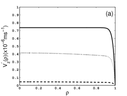
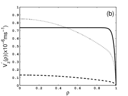
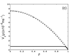
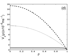
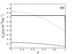
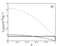
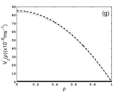
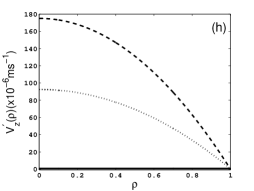
Figure 1: Variation of $V_{z}^{\prime}(\rho)$ with $\rho$ when (a–d) $m_{o}=50$ or (e–h) $m_{o}=500$, for $k_{1}=0$ (solid curves), $k_{1}=0.5$ (dotted curves), and $k_{1}=0.95$ (dashed curves). (a, e) $\beta_{o}=-0.01$, (b, f) $\beta_{o}=-0.1$, (c, g) $\beta_{o}=-0.95$, (d, h) $\beta_{o}=-1$.

Figure 1 also shows that the speed of a micropolar fluid ($k_{1}\neq 0$) decreases as $k_{1}$ increases for all $m_{o}$ but not for all $\beta_{o}$. In addition to the fluid speed increasing with $m_{o}$ (just as for a simple Newtonian fluid), the fluid speed also increases with $|\beta_{o}|$ for all $m_{o}\gg 1$ and $k_{1}>0$.

The foregoing trends are in accord with the results of an analytical investigation in the central portion of the microcapillary. With the assumption that $m_{o}\geq 10$, Eq. (43) yields

$$V^{\prime}_{z}(0)\simeq U\left(1+k_{1}\left\{\frac{k_{2}}{k_{0}^{2}-m_{o}^{2}}-\frac{m_{o}}{k_{0}}\left(\frac{k_{2}}{k_{0}^{2}-m_{o}^{2}}+\frac{\beta_{o}}{1+k_{1}\beta_{o}}\right)\left[\frac{I_{0}(k_{0})-1}{I_{1}(k_{0})}\right]\right\}\right)\,.$$ (47)

For simple Newtonian fluids ($k_{1}=0$), Eq. (47) shows that $V^{\prime}_{z}(0)=U$ is independent of $m_{o}$ as well as of, as expected, $\beta_{o}$. Plots of $V^{\prime}_{z}(0)$ vs. $m_{o}$ in Figure 2 indicate that the fluid speed at the center of the microcapillary increases with $m_{o}$, and therefore with $R$, for micropolar fluids ($k_{1}\neq 0$). When microrotation effects can be neglected at the wall of the microcapillary—i.e., when $\beta_{o}=0$—Eq. (47) simplifies to

$$V^{\prime}_{z}(0)\Big{|}_{\beta_{o}=0}\simeq U\left(1+\frac{k_{1}k_{2}}{k_{0}^{2}-m_{o}^{2}}\left\{1-\left(\frac{m_{o}}{k_{0}}\right)\left[\frac{I_{0}(k_{0})-1}{I_{1}(k_{0})}\right]\right\}\right)\,,$$ (48)

and Figure 2 shows that the effect of $m_{o}$ on $V^{\prime}_{z}(0)$ is very weak but the effect of $k_{1}$ is considerable. As $|\beta_{o}|$ increases, $V^{\prime}_{z}(0)$ acquires a stronger tendency in a micropolar fluid to increase with $m_{o}$, which can be concluded from Figure 2.

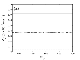
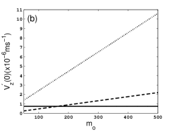
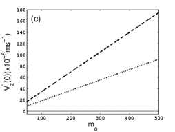
Figure 2: Variation of $V_{z}^{\prime}(0)$ with $m_{o}$ for $k_{1}=0$ (solid curves), $k_{1}=0.5$ (dotted curves), and $k_{1}=0.95$ (dashed curves). (a) $\beta_{o}=0$, (b) $\beta_{o}=-0.2$, (c) $\beta_{o}=-1$.

The fluid-speed gradient ${dV_{z}^{\prime}}/{d\rho}$ is not only an important factor in microrotation per Eqs. (33)₁ and (37), but it also influences several components of the stress tensor identified in Eqs. (46). The Debye–Hückel expression for ${dV_{z}^{\prime}}/{d\rho}$ follows from Eqs. (36), (37), and (41) as

$$\frac{dV^{\prime}_{z}(\rho)}{d\rho}=-U\left[c_{1}k_{1}I_{1}(k_{0}\rho)+m_{o}\left(1+\frac{k_{1}k_{2}}{k_{0}^{2}-m_{o}^{2}}\right)\frac{I_{1}(m_{o}\rho)}{I_{0}(m_{o})}\right]\,.$$ (49)

Now, this gradient vanishes as $\rho\to 0$, i.e., at the centre of the microcapillary, in conformity with boundary condition (32). But it has high magnitudes near the wall, as can be gathered by setting $\rho=1$ in Eq. (49) to obtain

$$\frac{dV^{\prime}_{z}(\rho)}{d\rho}\Big{|}_{\rho=1}=-\frac{Um_{o}}{1+k_{1}\beta_{o}}\,\frac{I_{1}(m_{o})}{I_{0}(m_{o})}\,.$$ (50)

When $m_{o}\geq 10$, the foregoing expression can be further approximated as

$$\frac{dV^{\prime}_{z}(\rho)}{d\rho}\Big{|}_{\rho=1}\simeq-\frac{Um_{o}}{1+k_{1}\beta_{o}}\,,$$ (51)

evincing a direct proportionality with $m_{o}$ (or $R$) for all $|\beta_{o}|$—for both simple Newtonian and micropolar fluids.

4.2 Fluid flux

From an engineering perspective, the fluid flux should be considered in addition to fluid speed. In the present context, it is defined as

$$Q^{\prime}=2\pi\int^{R}_{0}\rho^{\prime}\,V^{\prime}_{z}(\rho^{\prime})\,{d\rho^{\prime}}=2\pi{R^{2}U}\int^{1}_{0}\rho\,V_{z}(\rho)\,d\rho\,.$$ (52)

On substituting the Debye–Hückel expression (43) in the integrand on the right side of Eq. (52), we get

$$Q^{\prime}={\pi}R^{2}U\left[\frac{c_{1}k_{1}}{k_{0}}I_{2}(k_{0})+\left(1+\frac{k_{1}k_{2}}{k^{2}_{0}-m^{2}_{o}}\right)\frac{I_{2}(m_{o})}{I_{0}(m_{o})}\right]\,,$$ (53)

which simplifies to

$$Q^{\prime}\simeq{\pi}R^{2}U\left[\frac{c_{1}k_{1}}{k_{0}}I_{2}(k_{0})+\left(1+\frac{k_{1}k_{2}}{k^{2}_{0}-m^{2}_{o}}\right)\left(1-\frac{2}{m_{o}}\right)\right]\,$$ (54)

for $m_{o}\geq 10$. Clearly then, the fluid flux depends on $k_{1}$, $\beta_{o}$, and $m_{o}$.

The dependence of $Q^{\prime}$ on $\beta_{o}$ can be identified using Eqs. (42) and (53). We can write $Q^{\prime}$ as the sum of two parts, one of which is independent of $\beta_{o}$ and the other depends linearly on $\beta_{o}/(1+k_{1}\beta_{o})$.

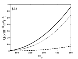
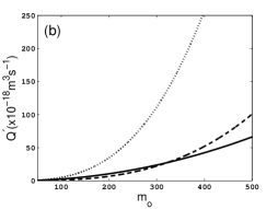
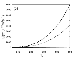
Figure 3: Variation of $Q^{\prime}$ with $m_{o}$ for $k_{1}=0$ (solid curves), $k_{1}=0.5$ (dotted curves), and $k_{1}=0.95$ (dashed curves). (a) $\beta_{o}=-0.01$, (b) $\beta_{o}=-0.2$, (c) $\beta_{o}=-1$.

Although for simple Newtonian fluids ($k_{1}=0$), Eq. (54) yields

$$1-\frac{Q^{\prime}}{{\pi}R^{2}U}\simeq\frac{2}{m_{o}}$$ (55)

for $m_{o}\gg 1$, the relationship of $Q^{\prime}$ and $m_{o}$ is more complicated when $k_{1}\neq 0$. The variation of ${Q^{\prime}}$ with respect to $m_{o}$ is illustrated in Figure 3 for nine different combinations of $k_{1}$ and $\beta_{o}$. This figure shows that $Q^{\prime}$ increases with $m_{o}$ (and, therefore, with $R$) for simple Newtonian fluids; the same trend exists for micropolar fluids, regardless of the value of $\beta_{o}\in[-1,0]$. Furthermore, $Q^{\prime}$ intensifies with increasing $|\beta_{o}|$ for all $m_{o}\in[50,500]$ and $k_{1}\in(0,1)$, the intensification rate $dQ^{\prime}/d|\beta_{o}|$ itself increasing concurrently.

Figure 4 shows the dependency of $Q^{\prime}$ on $k_{1}$ for 12 different combinations of $\beta_{o}$ and $m_{o}$. Above a threshold value of $|\beta_{o}|$ which is quite small, the following trend is followed: from the value $Q^{\prime}_{0}\simeq\pi{R^{2}}U(1-2/m_{o})$ at $k_{1}=0$, the fluid flux $Q^{\prime}$ increases linearly with $k_{1}$ for $k_{1}\ll 1$, then increases nonlinearly with $k_{1}$ to a maximum value ${\tilde{Q}}^{\prime}$ at $k_{1}={\tilde{k}}_{1}$, and finally drops monotonically to $Q^{\prime}_{1}$ at $k_{1}=1$, for $\beta_{o}\in(-1,0]$ and $m_{o}\gg 1$. Whereas ${\tilde{Q}}^{\prime}$ increases with both $m_{o}$ and $|\beta_{o}|$, ${\tilde{k}}_{1}$ is almost totally independent of $m_{o}$ but increases with $|\beta_{o}|$. Calculations show that $Q^{\prime}_{1}{\sim}m_{o}^{n}$, with the exponent $n$ lying between 2 and 3 and increasing with $|\beta_{o}|$. Furthermore, for $\beta_{o}=-1$, $Q^{\prime}$ increases linearly with $k_{1}$ for $k_{1}\in[0,1]$ and ${\tilde{k}}_{1}=1$.

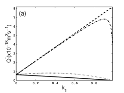
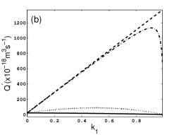
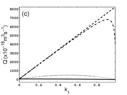
Figure 4: Variation of $Q^{\prime}$ with $k_{1}$ for $\beta_{o}=-0.01$ (solid curves), $\beta_{o}=-0.2$ (dotted curves), $\beta_{o}=-0.99$ (dashed-dotted curves), and $\beta_{o}=-1.0$ (dashed curves).(a) $m_{o}=50$, (b) $m_{o}=275$, and (c) $m_{o}=500$.

4.3 Microrotation

The microrotation $v^{\prime}_{\theta}(\rho)$ exists in micropolar fluids but not in simple Newtonian fluids. Accordingly, representative plots of $v^{\prime}_{\theta}$ vs. $\rho$, computed using the Debye–Hückel expression (41), are presented in Figure 5 for $m_{o}\gg 1$ and $k_{1}>0$. This figure indicates that $v^{\prime}_{\theta}(\rho)$

• increases linearly with $\rho$,

• increases with $|\beta_{o}|$ for all $k_{1}\in(0,1)$ and $\rho\in(0,1]$, and

• decreases as $k_{1}$ increases for all $m_{o}\in[50,500]$ and $\beta_{o}\in[-1,0)$.

By virtue of the boundary condition (33)₂, the microrotation is weak in the the central part of the microcapillary, but it is maximum at the wall $\rho=1$ for all $m_{o}\gg 1$, $\beta_{o}\in[-1,0)$, and $k_{1}>0$. Indeed, Eq. (41) yields

$$v^{\prime}_{\theta}(\rho)\Big{|}_{\rho=1}\approx-\frac{U\beta_{o}}{\lambda_{D}(1+k_{1}\beta_{o})}\,.$$ (56)

This equation shows that the microrotation at the wall of the microcapillary is independent of $R$f, which is in agreement with Figure 5. This figure also shows that, for $\beta_{o}=-1$, $v^{\prime}_{\theta}$ at $\rho=1$ is independent of $k_{1}$, which agrees with the result

$$v^{\prime}_{\theta}(\rho)\Big{|}_{\rho=1,\beta_{o}=-1}\approx-\frac{\epsilon\psi_{o}E_{o}}{\mu\lambda_{D}}\,.$$ (57)

obtained after using the definitions (13) and (18) in Eq. (56).

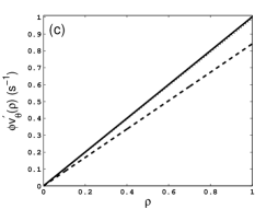
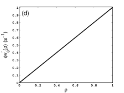
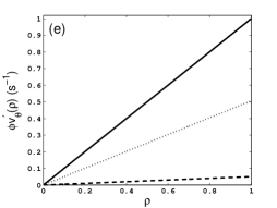
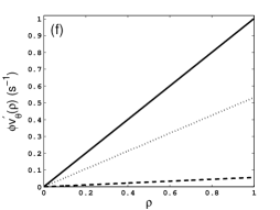
Figure 5: Variation of $\phi v^{\prime}_{\theta}(\rho)$, where the normalization factor $\phi=(68|\beta_{o}|)^{-1}$, with $\rho$ when (a–d) $m_{o}=50$ or (e–h) $m_{o}=500$, for $k_{1}=0.01$ (solid curves), $k_{1}=0.5$ (dotted curves), and $k_{1}=0.95$ (dashed curves). (a, e) $\beta_{o}=-0.001$, (b, f) $\beta_{o}=-0.1$, (c, g) $\beta_{o}=-0.99$, (d, h) $\beta_{o}=-1$.

All of the foregoing conclusions about the microrotation can be encapsulated as the approximation

$$v^{\prime}_{\theta}(\rho)\simeq-\frac{U}{R}\,\frac{\beta_{o}}{1+k_{1}\beta_{o}}\,m_{o}\rho\,,$$ (58)

which is valid for $m_{o}\gg 1$. Its derivation proceeds as follows: A comparison of magnitudes for large $m_{o}$ suggests that ${k_{2}}/\left(k_{0}^{2}-m_{o}^{2}\right)$ can be neglected in favor of ${\beta_{o}}/\left(1+k_{1}\beta_{o}\right)$ while $I_{1}(m_{o})/I_{0}(m_{o})\simeq 1$ in Eq. (42), leading to

$$c_{1}\simeq-\frac{\beta_{o}}{1+k_{1}\beta_{o}}\,m_{o}\frac{1}{I_{1}(k_{0})}\,.$$ (59)

A similar argument leads to the neglect of the second term on the right side of Eq. (41)  yielding

$$v_{\theta}(\rho)\simeq-\frac{\beta_{o}}{1+k_{1}\beta_{o}}\,m_{o}\frac{I_{1}(k_{0}\rho)}{I_{1}(k_{0})}\,.$$ (60)

Even for very large $m_{o}$, $k_{0}$ is very small so that $I_{1}(k_{0})\simeq k_{0}/2$ and $I_{1}(k_{0}\rho)\simeq k_{0}\rho/2$; Eq. (58) then follows for $m_{o}\gg 1$.

4.4 Stress tensor

After the use of Eqs. (41) and (43) in Eqs. (45)₁ and (45)₂, we obtain the non-zero components of the stress tensor as

$$\sigma^{\prime}_{\rho{z}}(\rho)=\frac{\epsilon\psi_{o}E_{o}}{\lambda_{D}}\frac{I_{1}(m_{o}\rho)}{I_{0}(m_{o})}$$ (61)

and

$$\sigma^{\prime}_{z\rho}(\rho)=\frac{\epsilon\psi_{o}E_{o}}{\lambda_{D}}\left\{\frac{c_{1}k_{1}\left(2-k_{1}\right)}{m_{o}}I_{1}(k_{0}\rho)+\left[1+\frac{k_{1}m_{o}^{2}}{k^{2}_{0}-m^{2}_{o}}\right]\frac{I_{1}(m_{o}\rho)}{I_{0}(m_{o})}\right\}\,,$$ (62)

consistently with the Debye–Hückel approximation. For a simple Newtonian fluid ($k_{1}=0$), from the foregoing expressions we get $\sigma^{\prime}_{\rho{z}}(\rho)=\sigma^{\prime}_{{z}\rho}(\rho)$, which conforms to the symmetry of the stress tensor in the absence of micropolarity. In a micropolar fluid ($k_{1}\neq 0$), the stress tensor of Eq. (1) has both symmetric and skew-symmetric components, which explains why $\sigma^{\prime}_{\rho{z}}(\rho)\neq\sigma^{\prime}_{{z}\rho}(\rho)$.

What is really surprising is that $\sigma^{\prime}_{\rho{z}}(\rho)$ is the same for simple Newtonian as well as micropolar fluids. This component of the stress tensor depends on $m_{o}$, but neither on $k_{1}$ nor on $\beta_{o}$. Furthermore, per Eq. (61), it is absent on the axis of the microcapillary because $I_{1}(0)=0$. Indeed, as can be deduced from Fig. 6, $\sigma^{\prime}_{\rho{z}}(\rho)$ is negligible in most of the microcapillary and becomes significant in magnitude very near to and on the wall, with

$$\sigma^{\prime}_{\rho{z}}(\rho)\Big{|}_{\rho=1}=\frac{\epsilon\psi_{o}E_{o}}{\lambda_{D}}\,.$$ (63)

As $m_{o}$ increases, the region in which the magnitude of $\sigma^{\prime}_{\rho{z}}(\rho)$ is significant shrinks.

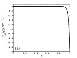
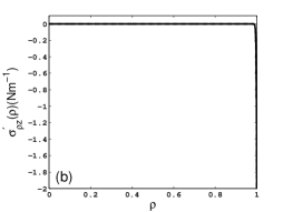
Figure 6: Variation of $\sigma^{\prime}_{\rho z}(\rho)$ with $\rho$ when (a) $m_{o}=50$ or (b) $m_{o}=500$. There is no dependence on either $k_{1}$ or $\beta_{o}$.

The difference $\sigma^{\prime}_{\rho{z}}(\rho)-\sigma^{\prime}_{z\rho}(\rho)$ is entirely due to micropolaity, as becomes evident on comparing the spatial profiles of $\sigma^{\prime}_{z\rho}(\rho)$ in Fig. 7 with the spatial profiles of $\sigma^{\prime}_{\rho{z}}(\rho)$ in Fig. 6. Clearly, $\sigma^{\prime}_{z\rho}(\rho)$ depends on $m_{o}$, $k_{1}$, and $\beta_{o}$. Now, $\sigma^{\prime}_{z\rho}(0)=0$ but

$$\sigma^{\prime}_{z\rho}(\rho)\Big{|}_{\rho=1}\approx\frac{\epsilon\psi_{o}E_{o}}{\lambda_{D}}\,\frac{(1-k_{1}-k_{1}\beta_{o})}{(1+k_{1}\beta_{o})}\left(1-\frac{1}{2m_{o}}\right)\,$$ (64)

for $m_{o}\gg 1$, and Fig. 7 shows that $\sigma^{\prime}_{z\rho}(0)>\sigma^{\prime}_{z\rho}(\rho)>\sigma^{\prime}_{z\rho}(1)$ for $\rho\in(0,1)$. The region around the central axis of the microcapillary can be called a $\sigma^{\prime}_{z\rho}$–free zone, which shrinks rapidly as $|\beta_{o}|$ increases.

Figure 7 also shows that $|\sigma^{\prime}_{z\rho}|$ not only increases with $k_{1}$ for $m_{o}\gg 1$ but it also increases with $m_{o}\gg 1$ for all $k_{1}\in[0,1]$ and $\beta_{o}\in(-1,0)$. As $\beta_{o}\rightarrow 0$, the distinction between the micropolar and the simple Newtonian fluids disappears for $\sigma^{\prime}_{z\rho}(\rho)$.

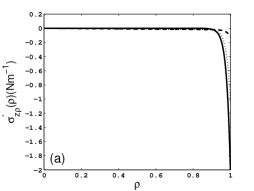
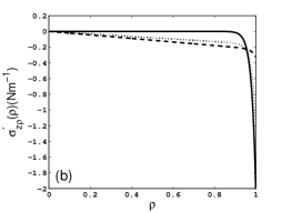
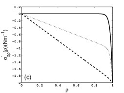
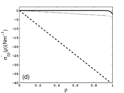
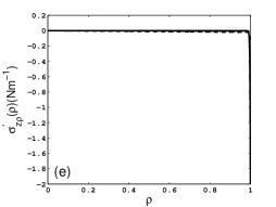
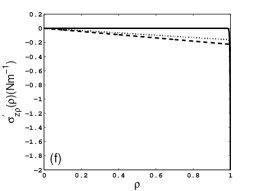
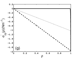
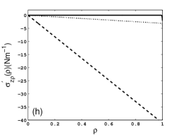
Figure 7: Variation of $\sigma^{\prime}_{z\rho}(\rho)$ with $\rho$ when (a–d) $m_{o}=50$ or (e–h) $m_{o}=500$, for $k_{1}=0$ (solid curves), $k_{1}=0.5$ (dotted curves), and $k_{1}=0.95$ (dashed curves). (a, e) $\beta_{o}=-0.001$, (b, f) $\beta_{o}=-0.1$, (c, g) $\beta_{o}=-0.5$, (d, h) $\beta_{o}=-1$.

4.5 Couple stress tensor

The couple stress arises in conjunction with the microrotation, as delineated by Eq. (2), and therefore cannot exist in a simple Newtonian fluid. Consistently with the approximations made for a microcapillary, the only two non-zero components of the couple stress tensor are given by Eqs. (45)_3,4 or, equivalently, Eqs. (46)_3,4. Substitution of the Debye–Hückel approximation (41) for $v_{\theta}$ therein yields

$$m^{\prime}_{\rho\theta}(\rho)=\frac{\gamma{U}}{R^{2}}\left\{c_{1}\left[k_{0}k_{7}I_{0}(k_{0}\rho)-\frac{k_{7}+1}{\rho}I_{1}(k_{0}\rho)\right]\right.$$

$$\qquad\qquad\left.+k_{8}\left[m_{o}k_{7}I_{0}(m_{o}\rho)-\frac{k_{7}+1}{\rho}I_{1}(m_{o}\rho)\right]\right\}\,$$ (65)

and

$$m^{\prime}_{\theta\rho}(\rho)=\frac{\gamma{U}}{R^{2}}\left\{c_{1}\left[k_{0}I_{0}(k_{0}\rho)-\frac{k_{7}+1}{\rho}I_{1}(k_{0}\rho)\right]\right.$$

$$\qquad\qquad\left.+k_{8}\left[m_{o}I_{0}(m_{o}\rho)-\frac{k_{7}+1}{\rho}I_{1}(m_{o}\rho)\right]\right\}\,,$$ (66)

where

$$k_{8}=\frac{k_{2}}{k_{0}^{2}-m_{o}^{2}}\,\frac{m_{o}}{I_{0}(m_{o})}\,.$$ (67)

Equations (65) and (66) yield the difference

$$m^{\prime}_{\rho\theta}(\rho)-m^{\prime}_{\theta\rho}(\rho)=\frac{\gamma{U}}{R^{2}}\left(k_{7}-1\right)\left[c_{1}k_{0}I_{0}(k_{0}\rho)+k_{8}m_{o}I_{0}(m_{o}\rho)\right]\,$$ (68)

between the two non-zero components of $\underline{\underline{m}}^{\prime}$. This difference vanishes for all $\rho\in\left[0,1\right]$ when $\beta=\gamma$ (i.e., $k_{7}=1$), in agreement with Eq. (2). Furthermore, as

$$m^{\prime}_{\rho\theta}(0)=-m^{\prime}_{\theta\rho}(0)=\frac{\gamma{U}}{2R^{2}}\left(k_{7}-1\right)\left(c_{1}k_{0}+k_{8}m_{o}\right)\,,$$ (69)

the condition $\beta=\gamma$ also implies that the couple stress tensor is nonexistent on the axis of the microcapillary.

A more general but slightly approximate conclusion can be drawn from Eq. (58) for $m_{o}\gg 1$ as follows. That equation yields $v_{\theta}(\rho)\simeq-{\beta_{o}}\left({1+k_{1}\beta_{o}}\right)^{-1}m_{o}\rho$, whose use in Eqs. (46)_3,4 and (12) provides

$$m^{\prime}_{\rho\theta}(\rho)=-m^{\prime}_{\theta\rho}(\rho)\simeq-\frac{\gamma{U}}{R^{2}}(k_{7}-1)\frac{m_{o}\beta_{o}}{1+k_{1}\beta_{o}}$$ (70)

for $m_{o}\gg 1$. In other words, the couple stress tensor is skew-symmetric as well as uniform throughout the cross-section of the microcapillary. The approximate equations (70) were verified by directly using Eqs. (65) and (66) to plot the variations of $m^{\prime}_{\rho\theta}(\rho)$ and $m^{\prime}_{\theta\rho}(\rho)$ with $\rho$ in Figs. 8 and 9, respectively.

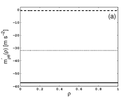
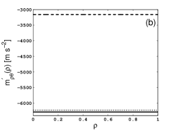
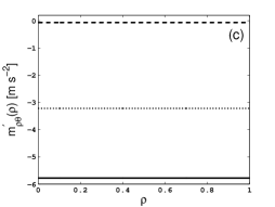
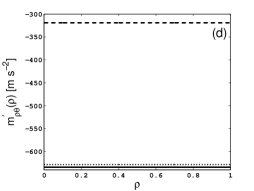
Figure 8: Variation of $m^{\prime}_{\rho\theta}(\rho)$ with $\rho$ when $k_{7}=0.5$ and (a,b) $m_{o}=50$ or (c,d) $m_{o}=500$, for $k_{1}=0.1$ (solid curves), $k_{1}=0.5$ (dotted curves), and $k_{1}=0.99$ (dashed curves). (a, c) $\beta_{o}=-0.01$, (b, d) $\beta_{o}=-0.99$.

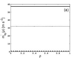
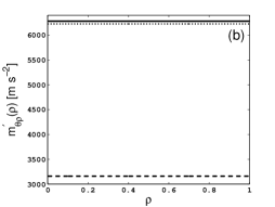
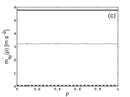
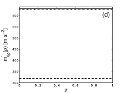
Figure 9: Same as Fig. 8, except that $m^{\prime}_{\theta\rho}(\rho)$ is plotted against $\rho$.

5 CONCLUDING REMARKS

We formulated the boundary-value problem of steady electro-osmotic flow of a micropolar fluid in a microcapillary whose length is much greater than its cross-sectional radius. Analytical solution of this boundary-value problem was obtained under the assumption that both the Debye length and the zeta potential are sufficiently small in magntitude so that the Debye–Hückel approximation could be used.

As the aciculate particles in a micropolar fluid can rotate without translation, micropolarity must influence fluid speed. The derived expressions and the calculated data indicate that the fluid speed depends significantly on the viscosity coupling parameter $k_{1}$, which mediates the (micropolar) viscosity coefficient and Newtonian shear viscosity coefficient. The axial speed of a micropolar fluid is below the speed of a simple Newtonian fluid for small values of the micropolar boundary parameter $\beta_{o}$—which relates the velocity gradient and microrotation at the wall of the microcapillary—but exceeds the latter for $\beta_{o}$ close to $-1$. In addition, the axial speed is independent of the radius of the microcapillary when the fluid if of simple Newtonian type but not when it is micropolar, provided the Debye length is fixed; indeed, the magnitude of the axial speed in a micropolar fluid intensifies as the radius increases.

The fluid flux increases as either the microcapillary radius increases and/or the Debye length decreases, whether the fluid is simple Newtonian or micropolar—in the latter case, regardless of the value of the micropolar boundary parameter $\beta_{o}$. The flux of a micropolar fluid increases as the magnitude of that boundary parameter intensifies.

Although microrotation greatly influences the speed and the flux, it vanishes on the axis of the microcapillary and increases linearly in the radial direction. Microtation increases with the magnitude of the micropolar boundary parameter $\beta_{o}$, but it decreases as the viscosity coupling parameter $k_{1}$ increases. Quite surprisingly, microrotation at the wall is independent of the cross-sectional radius of the microcapillary. Moreover, when the boundary layer is turbulent (i.e., $\beta_{o}=-1$), microrotation at the wall is also independent of $k_{1}$.

The stress tensor in the fluid has just two non-zero components, one of which is totally unaffected by the micropolarity of the fluid. That component does not exist on the axis and is largely confined to the region close to the wall. The other component is also absent on the axis and it gets progressively concentrated on the region close to the wall as $\beta_{o}\to-1$.

Unlike all foregoing physical parameters, both non-zero components of the skew-symmetric couple stress tensor are uniform in a micropolar fluid throughout the cross-section of the microcapillary. The couple stress tensor does not exist in a simple Newtonian fluid.

Our conclusions are significant for the design of microcapillaries are the selection of materials for labs-on-a-chip. For instance, turbulence caused by mixing of a (micropolar) body fluid with a (simple Newtonian) reagent fluid is likely to result in higher electro-osmotically induced flux and axial speed in a microcapillary than if both fluids are of the simple Newtonian type, suggesting that the microcapillary be designed with a larger cross-sectional diameter. Higher stress at the wall of a microcapillary transporting a micropolar fluid suggests that stiffer materials be used for the construction of labs-in-a-chip than if all fluids were to be simple Netwonian. As all of our conclusions apply when the zeta potential is sufficiently small in magnitude and the the cross-sectional radius of the microcapillary exceeds the Debye length, numerical solution of Eqs. (6)–(8) is required for more general situations. We plan to take up that investigation next.

References

[1] Arangoa M A, Campanero M A, Popineau Y and
Irache J M 1999 Electrophoretic separation and
characterisation of gliadin fractions from isolates and
nanoparticulate drug delivery systems, Chromatographia50
243–246.
[2] Fluri K, Fitzpatrick G, Chiem N and Harrison
D J 1996 Integrated capillary electrophoresis devices with an
efficient postcolumn reactor in planar quartz and glass chips,
Anal. Chem.68 4285–4290.
[3] DeCourtye D, Sen M and Gad-el-Hak M 1998
Analysis of viscous micropumps and microturbines, Int. J. Comp.
Fluid Dynam.10 13–25.
[4] Fan Z H and Harrison D J 1994 Micromachining
of capillary electrophoresis injectors and separators on glass chips
and evaluation of flow at capillary intersections, Anal. Chem.66 177–184.
[5] Harrison D J, Manz A and Glavina P G 1991
Electroosmotic pumping within a chemical sensor system integrated on
silicon, Proc. TRANSDUCERS ’91: 1991 Int. Conf. Solid–State Sens.
Actuat. 792–795.
[6] Keane M A 2003 Advances in greener separation
processes—case study: recovery of chlorinated aromatic compounds,
Green Chem.5 309–317.
[7] Murugan M, Rajanbabu K, Tiwari S A,
Balasubramanian C, Yadav M K, Dangore A Y, Prabhakar S
and Tewari P K 2006 Fouling and cleaning of seawater reverse
osmosis membranes in Kalpakkam nuclear desalination plant, Int. J.
Nucl. Desalination2 172–178.
[8] Probstein R F 1989 Physicochemical
Hydrodynamics: An Introduction (Stoneham, MA: Butterworths).
[9] Debye P and Hückel E 1923 Zur Theorie der
Elektrolyte. I. Gefrierpunktserniedrigung und verwandte
Erscheinungen, Phys. Z.24 185–206.
[10] Ariman T, Turk M A and Sylvester N D 1973
Microcontinuum fluid mechanics—A review, Int. J. Eng. Sci.11
905–930.
[11] Eringen A C 1973 On nonlocal microfluid
mechanics, Int. J. Eng. Sci.11 291–306.
[12] Eringen A C 2001 Microcontinuum Field
Theories, Vol. 2: Fluent Media (New York: Springer).
[13] Misra J C and Ghosh S K 2001 A mathematical
model for the study of interstitial fluid movement vis-a-vis the
non-newtonian behaviour of blood in a constricted artery, Compu.
Maths. Appl.41 783–811.
[14] Turk M A, Sylvester N D and Ariman T
1973 On pulsatile blood flow, Trans. Soc. Rheol.17 1–21.
[15] Oosterbroek R E and van den Berg A (Eds.)
2003 Lab-on-a-chip: Miniaturized Systems for (Bio)Chemical
Analysis and Synthesis (Oxford: Elsevier).
[16] Siddiqui A A and Lakhtakia A 2009 Steady
electro-osmotic flow of a micropolar fluid in a microchannel, Proc.
R. Soc. Lond. A465 501–522.
[17] Siddiqui A A and Lakhtakia A 2009 Non-steady
electro-osmotic flow of a micropolar fluid in a microchannel, J.
Phys. A: Math. Theor.42 355501.
[18] Eijkel J C T and van den Berg A 2006 The
promise of nanotechnology for separation devices—from a top-down
approach to nature-inspired separation devices, Electrophoresis27 677–685.
[19] Riehemann K, Schneider S W, Luger T A, Godin
B, Ferrari M and Fuchs H 2009 Nanomedicine—Challenges and
perspectives, Angew. Chem. Int. Ed.48 872–897.
[20] Li D 2004 Electrokinetics in Microfluidics,
Vol. 2 (London: Elsevier).
[21] Papautsky I, Brazzle J, Ameel T and Frazier
A B 1999 Laminar fluid behavior in microchannel using
micropolar fluid theory, Sens. Actuat. A: Phys.73 101–108.
[22] Hegab H E and Liu G 2004 Fluid flow modeling
of micro-orifices using micropolar fluid theory, Proc. SPIE4177
257–267.
[23] Rees D A S and Bassom A P 1996 The Blasius
boundary-layer flow of a micropolar fluid, Int. J. Eng. Sci.34
113–124.
[24] Abramowitz M and Stegun I A (Eds) 1972 Handbook of
Mathematical Functions (New York, NY: Dover).
[25] Hunter R J 1988 Zeta Potential in Colloid
Science: Principles and Applications (San Diego, CA: Academic).