Orbital upper critical field and its anisotropy of clean one- and two-band superconductors

Abstract

The Helfand-Werthamer (HW) schemeHW of evaluating the orbital upper critical field is generalized to anisotropic superconductors in general, and to two-band clean materials, in particular. Our formal procedure differs from those in the literature; it reproduces not only the isotropic HW limit, but also the results of calculations for the two-band superconducting MgB₂MMK ; DS along with the existing data on $H_{c2}(T)$ and its anisotropy $\gamma(T)=H_{c2,ab}(T)/H_{c2,c}(T)$ ($a,c$ are the principal directions of a uniaxial crystal). Using rotational ellipsoids as model Fermi surfaces we apply the formalism developed to study $\gamma(T)$ for a few different anisotropies of the Fermi surface and of the order parameters. We find that even for a single band d-wave order parameter $\gamma(T)$ decreases on warming, however, relatively weakly. For order parameters of the form $\Delta(k_{z})=\Delta_{0}(1+\eta\cos k_{z}a)$,Xu according to our simulations $\gamma(T)$ may either increase or decrease on warming even for a single band depending on the sign of $\eta$. Hence, the common belief that the multi-band Fermi surface is responsible for the temperature variation of $\gamma$ is proven incorrect.

For two s-wave gaps, $\gamma$ decreases on warming for all Fermi shapes examined. For two order parameters of the form $\Delta(k_{z})=\Delta_{0}(1+\eta\cos k_{z}a)$ presumably relevant for pnictides, we obtain $\gamma(T)$ increasing on warming provided both $\eta_{1}$ and $\eta_{2}$ are negative, whereas for $\eta$’s $>0$, $\gamma(T)$ decreases. We study the ratio of the two order parameters at $H_{c2}(T)$ and find that the ratio of the small gap to the large one does not vanish at any temperature even at $H_{c2}(T)$, an indication that this does not happen at lower fields.

I Introduction

The seminal work of Helfand and Werthamer (HW)HW on the temperature dependence of the upper critical field $H_{c2}(T)$ is routinely applied to analyze data on new superconductors despite the fact that HW considered the isotropic s-wave case whereas in themajority of new materials both Fermi surfaces and order parameters are strongly anisotropic. The problem of $H_{c2}(T)$ has been studied theoretically for anisotropic situations as well: for layered systems,LNB for a few cases of hexagonal anisotropy of the Fermi surface and of the order parameter,Klemm1 for the two-band MgB₂, Gurevich1 ; MMK ; DS ; Gurevich2 ; Palistrant for d-wave cuprates, see. e.g., Ref. Maki, and references therein, and in a comprehensive work in Ref. Kita, , to name a few.

A ubiquitous feature of $H_{c2}$ in many new superconductors is the temperature dependent anisotropy parameter $\gamma=H_{c2,ab}/H_{c2,c}$ (for uniaxial materials), the property absent in conventional one-band isotropic s-wave materials. For example, $\gamma(T)$ of MgB₂ decreases on warming,Budko whereas for many Fe-based materials $\gamma(T)$ increases with increasing $T$.Budko-Canfield ; Gurevich3 ; China Up to date, the $T$ dependence of the anisotropy parameter $\gamma$ is considered by many to be caused by a multi-band character of the materials in question with the commonly given reference to the example of MgB₂. To our knowledge, no explanation was offered for the “unusual” $\gamma(T)$ of pnictides.

In this work we develop a method to evaluate both $H_{c2,c}(T)$ and $\gamma(T)$ that can be applied with minor modifications to various situations of different order parameter symmetries and Fermi surfaces, two bands included. Having in mind possible applications for data analysis, we provide only the necessary minimum of analytic developments resorting to numerical methods as soon as possible.

The upper critical field is affected by many factors: magnetic structures that may coexist or interfere with superconductivity, the paramagnetic limit, scattering, etc. In this work we have in mind to establish a qualitative picture of how the general features of anisotropic Fermi surfaces and order parameters affect $H_{c2}$ and its anisotropy, in particular.

Since the paramagnetic effects and the possibility of Fulde-Ferrel-Larkin-Ovchinnikov phase are not included in our scheme (one can find a comprehensive discussion of these questions in Ref. Gurevich2, ), applications to materials with high $H_{c2}(0)$ should be carried out with care; our results can prove useful for interpretation of data at temperatures where $H_{c2}(T)$ does not exceed the paramagnetic limit.

As far as applications to two-band materials are concerned, we note that our formalism applies only to superconductors with a single critical temperature $T_{c}$. More exotic possibilities of two component condensates with two distinct $T_{c}$’s are out of the scope of this paper; these are considered on general group-theoretical symmetry grounds, e.g., in Refs. Sigrist, ; Joynt, .

Fine details of Fermi surfaces are unlikely to strongly influence $H_{c2}(T)$ because, as is well-known and shown explicitly below, only the integrals over the whole Fermi surface enter equations for $H_{c2}(T)$. Circumstantial evidence for a weak connection between fine particularities of the Fermi surface and $H_{c2}(T)$ is provided by the very fact that the HW isotropic model works so well for many one-band s-wave materials, although their Fermi surfaces hardly resemble a sphere, take e.g. Nb. Another example is given by the calculations of Refs. DS, and MMK, for MgB₂ based on different model Fermi surfaces, but giving similar results reasonably close to the measured $H_{c2}(T)$. We, therefore, model actual Fermi surfaces of uniaxial materials of interest here by rotational ellipsoids (spheroids) choosing them as to have averaged squared Fermi velocities equal to the measured values or to those calculated for realistic Fermi surfaces. This idea, in fact, has been employed by Miranovic et al. for MgB₂.MMK Also, we tested our method on a rotational hyperboloid as an example of open Fermi surfaces, Appendix D. This work is still in progress. We intend to study more about effects of open Fermi surfaces (or two-band combinations of closed and open surfaces) on $H_{c2}(T)$.

We focus in this work on the clean limit for two major reasons. First, commonly after discovery of a new superconductor, an effort is made to obtain as clean single crystals as possible since those provide a better chance to study the underlying physics. Second, almost as a rule, new materials are multi-band so that the characterization of scattering leads to a multitude of scattering parameters which cannot be easily controlled or separately measured. Besides, in general, scattering suppresses the anisotropy of $H_{c2}$, the central quantity of interest in this work. We refer readers interested in effects of scattering to a number of successful dirty-limit microscopic models, e.g. to Ref. Gurevich1, and references therein.

In the next Section, we begin with the general discussion of the $H_{c2}$ problem for arbitrary Fermi surfaces and order parameters. We show that in the isotopic limit our approach is reduced to that of HW. The basic HW approach is then applied to anisotropic situations. The derivation involves rescaling of the coordinates and, therefore, necessitates co- and contravariant vectors representations. In our view, disregarding this necessity may lead to incorrect conclusions. Another formal feature of our approach should be mentioned: we avoid the minimization relative to the actual coordinate dependence of the order parameter in the mixed state often employed to find $H_{c2}(T)$.MMK ; DS ; Rieck ; Maki ; Palistrant In this sense, our method is close to the original HW work that stresses that $H_{c2}(T)$ is actually an eigenvalue problem.

Next, we formulate the problem for two s-wave bands and show that along with $H_{c2}(T)$ and its anisotropy one can find the ratio of order parameters on two bands, a quantity that up to date has been studied only in zero-field. We then formulate the problem for two bands with order parameters of different symmetries. To show how the method actually works, we consider in detail one or two bands with Fermi surfaces as rotational ellipsoids. The method is demonstrated on the well-studied example of MgB₂.

The anisotropy parameter $\gamma$ is shown to depend on temperature even for the one-band case for other than s-wave order parameters. This dependence is weak the d-wave materials with closed Fermi surfaces, is stronger for open Fermi shapes, and is stronger yet for order parameters of the form $\Delta=\Delta_{0}(1+\eta\cos k_{z}a)$, one of the candidates for Fe-based materials.Xu Moreover, $\gamma(T)$ increases or decreases on warming depending on the sign of the coefficient $\eta$, in other words, on whether $\Delta$ is maximum or minimum at $k_{z}=0$. These results challenge the common belief that temperature dependence of $\gamma$ is always related to the multi-band topology of Fermi surfaces.

For two bands, after checking the method on MgB₂, we focus on situations with dominant inter-band coupling which is relevant for Fe-based materials. While in most cases we have considered, $H_{c2,c}(T)$ is qualitatively similar to the HW curve, the anisotropy parameter $\gamma(T)$ may show a non-monotonic $T$ dependence even for s-wave order parameters depending on the Fermi surface shapes and densities of states (DOS). Most interesting are the order parameters $\Delta=\Delta_{0}(1+\eta\cos k_{z}a)$ which yield nearly linear increase of $\gamma(T)$ on warming, a ubiquitous feature seen in many Fe-based superconductors.

II The problem of $\bm{H_{c2}}$

Our approach is basically that of HW, although formally the equations we solve for $H_{c2}(T)$ are different and can be applied to anisotropic and multi-band situations. To establish the link to HW, we start the discussion with the one-band case. The problem of the 2nd order phase transition at $H_{c2}$ is addressed here on the basis of linearized (the order parameter $\Delta\to 0$) quasiclassic Eilenberger equations.Eilenb For clean materials we have:

$$(2\omega+{\bm{v}}\cdot{\bm{\Pi}})\,f=2\Delta/\hbar\,,$$ (1)

$$\frac{\Psi}{2\pi T}\ln\frac{T_{c}}{T}=\sum_{\omega>0}^{\infty}\Big{(}\frac{\Psi}{\hbar\omega}-\langle\Omega\,f\rangle\Big{)}\,.$$ (2)

Here, ${\bm{v}}$ is the Fermi velocity, ${\bm{\Pi}}=\nabla+2\pi i{\bm{A}}/\phi_{0}$, ${\bm{A}}$ is the vector potential, and $\phi_{0}$ is the flux quantum. $\Delta({\bm{r}},{\bm{k}}_{F})$ is the order parameter that in general depends on the position ${\bm{k}}_{F}$ at the Fermi surface (or on ${\bm{v}}$). The function $f({\bm{r}},{\bm{v}},\omega)$ originates from Gor’kov’s Green’s function integrated over energy near the Fermi surface. Further, $N(0)$ is the total density of states at the Fermi level per spin; the Matsubara frequencies are $\omega=\pi T(2n+1)/\hbar$ with an integer $n$. The averages over the Fermi surface are shown as $\langle...\rangle$. The Eilenberger function $g=\sqrt{1-ff^{+}}=1$ at $H_{c2}$. The temperature $T$ is in energy units, i.e., $k_{B}=1$.

The self-consistency equation (2) is written for the general case of anisotropic gaps: $\Delta=\Psi({\bf r},T)\,\Omega({\bf k}_{F})$. The function $\Omega({\bf k}_{F})$ which determines the $\bm{k}_{F}$ dependence of $\Delta$ is normalized so that

$$\langle\Omega^{2}\rangle=1\,,$$ (3)

for details see, e.g., Ref. RC, . Eq. (2) corresponds to the factorizable coupling potential, $V(\bm{k},\bm{k}^{\prime})=V_{0}\Omega(\bm{k})\Omega(\bm{k}^{\prime})$. This popular approximationKad works well for one band materials with anisotropic coupling. We show in Sections V and VI how this convenient shortcut can be generalized to a multi-band case.

We now recast the self-consistency Eq. (2) by writing the solution of Eq. (1) in the form

$$f={2\over\hbar}\int_{0}^{\infty}d\rho\,e^{-\rho(2\omega+{\bf v}\cdot{\bm{\Pi}})}\Delta\,,$$ (4)

by using the identity

$${1\over\hbar\omega}={2\over\hbar}\int_{0}^{\infty}d\rho\,e^{-2\omega\rho}\,,$$ (5)

and by summing up over $\omega$:

$$-\Psi\ln t=\int_{0}^{\infty}\frac{du}{\sinh\,u}\Big{(}\Psi-\langle\Omega^{2}e^{-\rho{\bf v}\cdot{\bm{\Pi}}}\Psi\rangle\Big{)}\,,$$ (6)

where $u=2\pi T\rho/\hbar$ and $t=T/T_{c}$. Hence, we got rid of the summation over $\omega$, a convenient feature for further analysis.

The self-consistency Eq. (6) can be further rewritten in the form free of the divergent factor $1/\sinh u$ in the integrand. To this end, we integrate by parts the right-hand side (RHS) of Eq. (6) using $du/\sinh u=d\,\ln\tanh(u/2)$. The first term on the RHS diverges:

$$\int_{0}^{\infty}\frac{du}{\sinh u}\Psi=-\Psi\ln\tanh\frac{\pi T\rho}{\hbar}\Big{|}_{\rho\to 0}\,.$$ (7)

The second term transforms to:

$$- \Big{\langle}\Omega^{2}\Big{[}\ln\tanh\frac{\pi T\rho}{\hbar}\,e^{-\rho{\bf v}{\bm{\Pi}}}\Big{]}_{\rho=0}^{\infty}\Psi\Big{\rangle}$$ (8)

$$- \Big{\langle}\Omega^{2}{\bf v}{\bm{\Pi}}\int_{0}^{\infty}d\rho\,\ln\tanh\frac{\pi T\rho}{\hbar}e^{-\rho{\bf v}{\bm{\Pi}}}\Psi\Big{\rangle}\,.$$

The first term here and the contribution (7) cancel, and we obtain instead of Eq. (6):

$$\Psi\ln t=\int_{0}^{\infty}d\rho\,\ln\tanh\frac{\pi T\rho}{\hbar}\,\langle\Omega^{2}{\bf v}{\bm{\Pi}}\,e^{-\rho{\bf v}\cdot{\bm{\Pi}}}\Psi\rangle\,.$$ (9)

Here, the singularity at $\rho\to 0$ is integrable.

II.1 $\bm{H_{c2}}$ near $\bm{T_{c}}$

In this domain, the gradients $\Pi\sim\xi^{-1}\to 0$, and one can expand $\exp(-\rho{\bm{v}}{\bm{\Pi}})$ in the integrand (9) and keep only the linear term:

$$-\Psi\delta t=\frac{7\zeta(3)\hbar^{2}}{16\pi^{2}T_{c}^{2}}\,\langle\Omega^{2}({\bm{v}}\cdot{\bm{\Pi}})^{2}\Psi\rangle\,,$$ (10)

where $\int_{0}^{\infty}dx\,x\ln\tanh x=-7\zeta(3)/16$ with $\zeta(3)=1.202$. This is, in fact, the anisotropic version of the linearized Ginzburg-Landau (GL) equation

$$-\xi^{2}_{ik}\Pi_{i}\Pi_{k}\Psi=\Psi\,,$$ (11)

with

$$\xi^{2}_{ik}=\frac{7\zeta(3)\hbar^{2}}{16\pi^{2}T_{c}^{2}\tau}\,\langle\Omega^{2}v_{i}v_{k}\rangle\,,\qquad\tau=1-t\,,$$ (12)

the result of Gor’kov and Melik-Barkhudarov.Gorkov Solving the eigenvalue problem for Eq. (11) which is similar to one for a charged particle in uniform magnetic field, see e.g. work by Tilley,Tilley one finds the critical fields in two principal directions of uniaxial materials:

$$H_{c2,c}=\frac{8\pi\phi_{0}T_{c}^{2}\tau}{7\zeta(3)\hbar^{2}\langle\Omega^{2}v_{a}^{2}\rangle}\,,$$

$$H_{c2,a}=\frac{8\pi\phi_{0}T_{c}^{2}\tau}{7\zeta(3)\hbar^{2}\sqrt{\langle\Omega^{2}v_{a}^{2}\rangle\langle\Omega^{2}v_{c}^{2}\rangle}}\,,$$ (13)

so that

$$\gamma^{2}(T_{c})=\left(\frac{H_{c2,a}}{H_{c2,c}}\right)^{2}=\frac{\xi_{aa}^{2}}{\xi_{cc}^{2}}=\frac{\langle\Omega^{2}v_{a}^{2}\rangle}{\langle\Omega^{2}v_{c}^{2}\rangle}\,.$$ (14)

The angular dependence

$$H_{c2}(\theta)=\frac{H_{c2,a}}{\sqrt{\sin^{2}\theta+\gamma^{2}\cos^{2}\theta}}\,$$ (15)

is a direct consequence of Eq. (11) in which $\xi^{2}_{ik}$ is a second rank tensor ($\theta$ is the angle between the applied field and the $c$ axis). We argue below that Eq. (11) holds at $H_{c2}$, in fact, at all temperatures, and so should the angular dependence (15), the common practice to call it “GL” notwithstanding. We show that this angular dependence holds for any order parameter symmetry and for any Fermi surface shape including two-band situations. These conclusions are, in fact, confirmed experimentallyTerashima ; Yuan ; Cedomir ; CeIrIn5 ; HHW1 ; HHW2 ; Choi1 and by calculations of Ref. MMK, .

III Isotropic gap on a Fermi sphere

This problem has been solved by HW for the whole curve $H_{c2}(T)$.HW It is instructive and useful for the following generalization to the anisotropic case to reproduce their result within the quasiclassic scheme.coherence

It was established in Ref. HW, that at $H_{c2}(T)$ at any temperature, the order parameter satisfies a linear equation

$$-\xi^{2}\Pi^{2}\Delta=\Delta$$ (16)

in which $\xi(T)$ should be determined so as to satisfy the self-consistency equation. One can see that this equation is equivalent to the Schroedinger equation for a charge moving in uniform magnetic field and that the maximum field in which non-trivial solutions $\Delta$ exist is $H_{c2}=\phi_{0}/2\pi\xi^{2}$. For the field along $z$ we choose the gauge $A_{y}=Hx$. One readily verifies that in terms of operators

$$\Pi^{\pm}=\Pi_{x}\pm i\Pi_{y},\quad\Pi_{x} = \partial_{x},\quad\Pi_{y}=\partial_{y}+iq^{2}x,$$

$$q^{2} = 2\pi H/\phi_{0}\,,$$ (17)

Eq. (16) reads $\Pi^{+}\Pi^{-}\Delta=0$ provided $q^{2}=1/\xi^{2}$. Therefore, we obtain a useful property of $\Delta$ at $H_{c2}(T)$:

$$\Pi^{-}\Delta=\Pi^{-}\Psi=0\,.$$ (18)

We now introduce $v^{\pm}=v_{x}\pm iv_{y}$ so that ${\bm{v}}{\bm{\Pi}}=(v^{-}\Pi^{+}+v^{+}\Pi^{-})/2$ and evaluate the average $\Big{\langle}{\bm{v}}{\bm{\Pi}}\,e^{-\rho{\bm{v}}{\bm{\Pi}}}\,\Psi\Big{\rangle}$ needed in the self-consistency Eq. (9). To this end, we use the known property of exponential operators:

$$e^{-\rho{\bm{v}}{\bm{\Pi}}}\,\Psi=e^{P+Q}\,\Psi=e^{P}e^{Q}e^{[Q,P]/2}\,\Psi\,.$$ (19)

Here, $P=-\rho v^{-}\Pi^{+}/2$, $Q=-\rho v^{+}\Pi^{-}/2$, the commutator $[Q,P]/2=-\rho^{2}v_{\perp}^{2}/4\xi^{2}$, and $v_{\perp}^{2}=v_{x}^{2}+v_{y}^{2}$.

Since $\Pi^{-}\Psi=0$ and $e^{Q}\Psi=\Psi$, we have:

$${\bm{v}}{\bm{\Pi}}e^{-\rho{\bm{v}}{\bm{\Pi}}}\Psi = {e^{-\eta}\over 2}(v^{-}\Pi^{+}+v^{+}\Pi^{-})\sum_{n=0}^{\infty}\frac{(-\rho v^{-}\Pi^{+})^{n}}{2^{n}n!}\Psi,$$

$$\eta = \frac{\rho^{2}v_{\perp}^{2}}{4\xi^{2}}\,.$$ (20)

After averaging over the Fermi sphere, only $\langle v^{+}v^{-}\rangle$ survives (use $v^{\pm}=v_{\perp}e^{\pm i\phi}$):

$$\big{\langle}{\bm{v}}{\bm{\Pi}}\,e^{-\rho{\bm{v}}{\bm{\Pi}}}\,\Psi\big{\rangle}=-{\rho\over 2}\big{\langle}e^{-\eta}v^{+}v^{-}\big{\rangle}\Pi^{-}\Pi^{+}\Psi\,.$$ (21)

Now, with the help of Eq. (16), the self-consistency Eq. (9) yields:

$$\xi^{2}\ln t={1\over 2}\int_{0}^{\infty}d\rho\,\rho\,\ln\tanh\frac{\pi T\rho}{\hbar}\,\left\langle e^{-\eta}v_{\perp}^{2}\right\rangle\,.$$ (22)

Introducing the dimensionless field

$$h=\frac{\hbar^{2}v_{F}^{2}}{4\pi^{2}T_{c}^{2}\xi^{2}}\,.$$ (23)

and a variable $s=\pi T_{c}\rho/\hbar$, we rewrite Eq. (22) for $\xi(t)$ as an equation for $h(t)$:

$$\ln t=2h\int_{0}^{\infty}ds\,s\,\ln\tanh(st)\left\langle\mu e^{-\mu hs^{2}}\right\rangle\,,$$ (24)

where $\mu=v_{\perp}^{2}/v_{F}^{2}$ and $v_{F}$ is the Fermi velocity. The field $h$ is the upper critical field in units of $\phi_{0}/(\hbar^{2}v_{F}^{2}/2\pi T_{c}^{2})$. Thus, solving Eq. (24) with respect to $h(t)$ we have the HW solution of the problem for the isotropic one-band case. In the following we refer to Eq. (24) as the HW result although in the original work they obtained a different form of the equation for $H_{c2}(T)$.

At arbitrary $T$, Eq. (24) can be solved numerically; the exceptions are $T\to 0$ and $T\to T_{c}$. Since $h(0)$ is finite, the integral over $s$ is truncated at $s\sim 1/\sqrt{\mu h}$; therefore, for low enough $t$ we have $\ln\tanh(st)\approx\ln t+\ln s$. The integration over $s$ then yields:

$${{\bf C}\over 2}=\Big{\langle}\ln\frac{2\pi T_{c}\xi(0)}{\hbar v_{\perp}}\,\Big{\rangle}\,,$$ (25)

where ${\bf C}=0.577$ is the Euler constant. The averaging over the Fermi sphere with $v_{\perp}=v_{F}\sin\theta$ is readily done:

$$\xi^{2}(0)=\frac{\hbar^{2}v_{F}^{2}}{2\pi^{2}T_{c}^{2}}\,e^{\bm{C}-2}\,.$$ (26)

Thus, we obtain:

$$H_{c2}(0)=\frac{\phi_{0}}{2\pi\xi^{2}(0)}=\frac{\phi_{0}\pi T_{c}^{2}}{2\hbar^{2}v_{F}^{2}}\,e^{2-{\bf C}}\,,$$ (27)

the value obtained variationally by Gor’kovgorkov and proven to be exact by HW.

Close to $T_{c}$, $H_{c2}$ is obtained as isotropic limits of Eqs. (13). It is instructive, however, to see how this can be deduced directly from Eq. (24). In this domain, $\ln t\approx t-1=-\tau$ and $h\propto\tau$. Then, the integral in Eq. (24) should be evaluated in zero order in $\tau$, in other words, $h$ in $\exp(-\mu hs^{2})$ can be set zero. Integration over $s$ gives $-(7\zeta(3)/16)\langle\mu\rangle$, whereas $\langle\mu\rangle=\langle v^{2}_{\perp}/v_{F}^{2}\rangle=2/3$:

$$h=12\,\tau/7\zeta(3)\,.$$ (28)

The reduced HW field

$$h^{*}(0)={H_{c2}(0)\over|H_{c2}^{\prime}(T_{c})|T_{c}}=\frac{h(0)}{|h^{\prime}(1)|}=\frac{7\zeta(3)e^{2}}{48\,e^{{\bf C}}}\approx 0.727,\qquad\quad$$ (29)

the correct HW value.

IV Anisotropic one-band case

The central point of the HW paper is the proof that the linearized GL equation (16) holds not only near $T_{c}$ but along the whole curve $H_{c2}(T)$. For anisotropic materials Eq. (16) should be replaced with Eq. (11) where all components of the tensor $(\xi^{2})_{ik}$ should be determined from the self-consistency equation. We consider here uniaxial materials for which the symmetric tensor $\xi_{ik}^{2}$ has two independent eigenvalues. One has for the field along one of the principal crystal directions which we call $z$:

$$-(\xi_{xx}^{2}\Pi_{x}^{2}+\xi_{yy}^{2}\Pi_{y}^{2})\Delta=\Delta\,.$$ (30)

We denote $\xi_{xx}=\xi/\sqrt{m_{x}}$, $\xi_{yy}=\xi/\sqrt{m_{y}}$, $\xi_{zz}=\xi/\sqrt{m_{z}}$ with dimensionless constants $m_{x,y,z}$. Since the three quantities, $\xi_{xx}$, $\xi_{yy}$, and $\xi_{zz}$ are replaced with four, $\xi$ and $m_{x,y,z}$, we can impose an extra condition: $m_{x}m_{y}m_{z}=1$. For uniaxial materials of interest here with $m_{c}\neq m_{a}=m_{b}$, we introduce the anisotropy parameter $\gamma=\sqrt{m_{c}/m_{a}}$, so that all “masses” are expressed in terms of $\gamma$: $m_{a}=\gamma^{-2/3}$, $m_{c}=\gamma^{4/3}$. It is worth noting that $m$’s here do not necessarily have the meaning of the band theory effective masses; rather, they are parameters describing the anisotropy of $H_{c2}$; near $T_{c}$ they can be expressed in terms of Fermi velocities and the gap anisotropy, Eq (14).Gorkov Hence, if the ansatz (11) is correct, the self-consistency equation must provide equations to determine $\xi(T)$ and $\gamma(T)$.

To make use of the property (18) in anisotropic situations we rescale coordinates in Eq. (30):

$$x^{\prime} = x\sqrt{m_{x}},\qquad y^{\prime}=y\sqrt{m_{y}}\,,$$ (31)

$$\frac{\partial^{2}\Delta}{\partial x^{\prime\,2}} + \Big{(}\frac{\partial}{\partial y^{\prime}}+iq^{\prime\,2}x^{\prime}\Big{)}^{2}\Delta=-\frac{\Delta}{\xi^{2}}\,,$$ (32)

$$q^{\prime\,2} = \frac{2\pi H}{\phi_{0}\sqrt{m_{x}m_{y}}}\,.$$ (33)

Formally, Eq. (32) is equivalent to the isotropic Eq. (16). The upper critical field is then determined by $q^{\prime\,2}=1/\xi^{2}$:

$$H_{c2}=\frac{\phi_{0}\sqrt{m_{x}m_{y}}}{2\pi\xi^{2}}\,.$$ (34)

Therefore, we have in the uniaxial case:

$$H_{c2,c}=\frac{\phi_{0}}{2\pi\xi^{2}}\,m_{a}\,,\qquad H_{c2,b}=\frac{\phi_{0}}{2\pi\xi^{2}}\sqrt{m_{a}m_{c}}\,$$ (35)

and

$$\frac{H_{c2,b}}{H_{c2,c}}=\sqrt{\frac{m_{c}}{m_{a}}}=\gamma\,.$$ (36)

Thus, the formally introduced “masses” are related to the measurable ratio of $H_{c2}$’s.

Any coordinate transformation results in transformation of vectors (and tensors). The scaling transformation (31) necessitates the co- and contravariant representations for vectors, see, e.g., Ref. LL2, or Morse, . The covariant gradients $\pi_{x}=\partial/\partial x^{\prime}$ and $\pi_{y}=\partial/\partial y^{\prime}+iq^{\prime\,2}x^{\prime}$ have the same properties as their isotropic counterparts $\Pi_{x,y}$. Eq. (32) acquires the “isotropic” form:

$$-\xi^{2}(\pi_{x}^{2}+\pi_{y}^{2})\Delta=\Delta\,,$$ (37)

$$\pi^{-}\pi^{+}\Delta=-2\Delta/\xi^{2}\,,\qquad\pi^{-}\Delta=0\,.$$ (38)

The following manipulation then is similar to what was done in the isotropic case; one, however, should keep track of differences between co- and contravariant components of vectors.

Since the scalar products are invariant, we have ${\bm{v}}{\bm{\Pi}}=\nu^{i}\pi_{i}=(\nu^{-}\pi^{+}+\nu^{+}\pi^{-})/2$, $\nu^{\pm}=\nu^{x}\pm i\nu^{y}$ where

$$\nu^{x}=v_{x}\sqrt{m_{x}}\,,\qquad\nu^{y}=v_{y}\sqrt{m_{y}}$$ (39)

are the contravariant components of the Fermi velocity that transform as coordinates, Eq. (31). Further, we use the property (19) of exponential operators with

$$P=-{\rho\over 2}\nu^{-}\pi^{+},\,Q=-{\rho\over 2}\nu^{+}\pi^{-},\,{1\over 2}[Q,P]=-\frac{\rho^{2}\nu_{\perp}^{2}}{4\xi^{2}},$$ (40)

and

$$\quad\nu_{\perp}^{2}=(\nu^{x})^{2}+(\nu^{y})^{2}=v_{x}^{2}m_{x}+v_{y}^{2}m_{y}\,.$$ (41)

Since $\pi^{-}\Psi=0$ and $e^{Q}\Psi=\Psi$, we have:

$${\bf v}{\bm{\Pi}}e^{-\rho{\bf v}{\bm{\Pi}}}\Psi$$

$$={e^{-\eta}\over 2}(\nu^{-}\pi^{+}+\nu^{+}\pi^{-})\sum_{n=0}^{\infty}\frac{(-\rho\nu^{-}\pi^{+})^{n}}{2^{n}n!}\Psi,$$ (42)

where $\eta=\rho^{2}\nu_{\perp}^{2}/4\xi^{2}$.

The next step in the “isotropic derivation” was to use the fact that $\langle v^{+}v^{-}\rangle=2v_{F}^{2}/3$ whereas all other averages (such as $\langle v^{+}v^{-}v^{-}\rangle$) vanish because $v^{\pm}=v_{\perp}e^{\pm i\phi}$ where $\phi$ is the azimuthal angle on a sphere. To prove rigorously that this is valid for a general Fermi surface is difficult, although it is probably true for uniaxial materials of interest here. As mentioned in the Introduction, to make progress in evaluation of $H_{c2}$ and its anisotropy we resort to modeling actual Fermi surfaces with spheroids. The rescaling employed above, in fact, transforms spheroids to “spheres” in rescaled coordinates so that we can still claim that the only surviving product after averaging of Eq. (42) is $\langle\nu^{+}\nu^{-}\rangle$ and we obtain:

$$\Big{\langle}\Omega^{2}\,{\bf v}{\bm{\Pi}}\,e^{-\rho{\bf v}{\bm{\Pi}}}\,\Psi\Big{\rangle}=-{\rho\over 2}\big{\langle}\Omega^{2}\,e^{-\eta}\nu^{+}\nu^{-}\big{\rangle}\pi^{-}\pi^{+}\Psi\,.$$ (43)

The self-consistency Eq. (9) now yields with the help of Eq. (38):

$$\xi^{2}\ln t={1\over 2}\int_{0}^{\infty}d\rho\,\rho\,\ln\tanh\frac{\pi T\rho}{\hbar}\,\langle\Omega^{2}e^{-\eta}\nu_{\perp}^{2}\rangle\,.$$ (44)

This equation (written for a certain field orientation) contains two unknown functions, $\xi(T)$ and $\gamma(T)$. Therefore, one has to write it for two field orientations: (a) for $\bm{H}$ along $c$ with $\eta=\rho^{2}\nu_{\perp}^{2}/4\xi^{2}$ and

$$\nu_{\perp}^{2}=m_{a}(v_{x}^{2}+v_{y}^{2})=\gamma^{-2/3}(v_{x}^{2}+v_{y}^{2})\,,$$ (45)

and (b) for $\bf H$ along $b$ with

$$\nu_{\perp}^{2}=m_{a}v_{x}^{2}+m_{c}v_{z}^{2}=\gamma^{-2/3}(v_{x}^{2}+\gamma^{2}v_{z}^{2})\,.$$ (46)

In principle, by solving the system of these two equations one can determine both $\xi(T)$ and $\gamma(T)$, thus proving the correctness of the ansatz (11).

Since the Fermi velocity is not a constant at anisotropic Fermi surfaces, we normalize velocities on some value $v_{0}$ for which we choose

$$v_{0}^{3}=\frac{2E_{F}^{2}}{\pi^{2}\hbar^{3}N(0)}\,,$$ (47)

where $E_{F}$ is the Fermi energy and $N(0)$ is the total density of states at the Fermi level per spin. One easily verifies that $v_{0}=v_{F}$ for the isotropic case.

We now write the self-consistency Eq. (44) for $\bm{H}\parallel\bm{c}$, i.e. with $\nu_{\perp}$ of Eq. (45), in dimensionless form. To this end, we go to the integration variable $s=\pi T_{c}/\hbar$, divide both parts by $\xi^{2}$, and multiply and divide the integrand by $v_{0}^{2}$:

$$\ln t = 2h_{c}\int_{0}^{\infty}s\,\ln\tanh(st)\,\left\langle\Omega^{2}\mu_{c}e^{-\mu_{c}h_{c}s^{2}}\right\rangle ds\,,\qquad$$ (48)

$$h_{c} = \frac{\hbar^{2}v_{0}^{2}\gamma^{-2/3}}{4\pi^{2}T_{c}^{2}\xi^{2}}\,,\qquad\mu_{c}=\frac{v_{x}^{2}+v_{y}^{2}}{v_{0}^{2}}\,.$$ (49)

One can see that $h_{c}$ is in fact $H_{c2,c}$ in units of $\phi_{0}/(\hbar^{2}v_{0}^{2}/2\pi T_{c}^{2})$. An important feature of Eq. (48) should be noted: it does not contain the anisotropy $\gamma$ explicitly so that it can be solved for $h_{c}(t)$.

Writing Eq. (44) for $\bm{H}\perp\bm{c}$ with $\nu_{\perp}$ of Eq. (46) we obtain:

$$\ln t=2h_{c}\int_{0}^{\infty}s\,\ln\tanh(st)\,\left\langle\Omega^{2}\mu_{b}e^{-\mu_{b}h_{c}s^{2}}\right\rangle ds\,,\qquad$$ (50)

$$\mu_{b}=\frac{v_{x}^{2}+\gamma^{2}v_{z}^{2}}{v_{0}^{2}}\,.\qquad\qquad\qquad\qquad$$ (51)

For the isotropic s-wave case, $\gamma=\Omega=1$ and Eqs. (48) and (50) coincide with each other and with Eq.(24) of HW. We note that the integrals on the RHS of Eqs. (48), (50) differ only in $\mu$’s; for brevity we denote:

$${\cal I}=\int_{0}^{\infty}s\,\ln\tanh(st)\,\left\langle\Omega^{2}\mu e^{-\mu h_{c}s^{2}}\right\rangle ds\,.$$ (52)

Thus, the general scheme for solving for $H_{c2}(T)$ and its anisotropy consists of (a) solving Eq. (48) for $h_{c}(t)$ and (b) for the now known $h_{c}(t)$, solving Eq. (50) for $\gamma(t)$.

IV.1 $\bm{T\to T_{c}}$ and $\bm{T\to 0}$

Analysis of Eqs. (48), (50) for arbitrary temperatures is difficult because $h_{c}(t)$ and $t$ enter the integrals $\cal I$ in a nonlinear fashion. The situation is simpler near $T_{c}$ where $\ln t\approx-\tau=t-1$ and $h_{c}\propto\tau$. Therefore, $\cal I$ can be evaluated in zero order in $\tau$, in other words, $h_{c}$ in the $\exp(-\mu^{2}_{c}h_{c}x^{2})$ can be set zero and $t=1$ in $\ln\tanh(xt)$. We obtain after integration:

$${\cal I}=-\frac{7\zeta(3)}{16}\Big{\langle}\Omega^{2}\mu\Big{\rangle}\,,\qquad$$ (53)

where for $\bm{H}\parallel\bm{c}$ one takes $\mu=\mu_{c}$ whereas $\mu=\mu_{b}$ for $\bm{H}\perp\bm{c}$. Eq. (48) now yields:

$$h_{c}=\frac{8\tau}{7\zeta(3)\left\langle\Omega^{2}\mu_{c}\right\rangle}\,,\quad h_{c}^{\prime}(1)=-\frac{8}{7\zeta(3)\left\langle\Omega^{2}\mu_{c}\right\rangle}\,.\qquad$$ (54)

It is readily shown that Eq. (50) for $\gamma(T_{c})$ reduces to

$$\Big{\langle}\Omega^{2}\mu_{b}\Big{\rangle}=\Big{\langle}\Omega^{2}\mu_{c}\Big{\rangle}\,.$$ (55)

Using $\mu_{b}$ and $\mu_{c}$ of Eqs. (51), (49) one reproduces the general result (14).

As $t\to 0$, $h_{c}\to$ const, and the exponential factor in $\cal I$ truncates the integrand at a finite $x\sim 1/\sqrt{\mu h_{c}}$. Hence, at small enough $t$, $\ln\tanh(xt)\approx\ln(xt)=\ln t+\ln x$. One can now integrate over $x$:

$${\cal I}(\mu)=\frac{\ln t}{2h_{c}}-\frac{{\bm{C}}+\left\langle\Omega^{2}\ln(h_{c}\mu)\right\rangle}{4h_{c}}\,.$$ (56)

Substituting this in Eq. (48) one obtains:

$$h_{c}(0)=\exp\left(-\bm{C}-\big{\langle}\Omega^{2}\ln\mu_{c}\big{\rangle}\right)\,.$$ (57)

The HW ratio for a general anisotropy reads:

$$h^{*}_{c}(0)=\frac{h_{c}(0)}{h_{c}^{\prime}(1)}=\frac{7\zeta(3)}{8e^{\bm{C}}}\left\langle\Omega^{2}\mu_{c}\right\rangle\exp\left(-\big{\langle}\Omega^{2}\ln\mu_{c}\big{\rangle}\right)\,.\qquad$$ (58)

Thus, the HW number $h^{*}(0)=0.727$ is corrected by both Fermi surface shape and by the order parameter symmetry.

Eq. (50) for $\gamma(0)$ along with expression for $h_{c}(0)$ readily gives at $T=0$:

$$\big{\langle}\Omega^{2}\ln\mu_{c}\big{\rangle}=\big{\langle}\Omega^{2}\ln\mu_{b}\big{\rangle}\,.$$ (59)

V Two s-wave bands

The general self-consistency equation for two bands reads:

$$\Delta_{\alpha}({\bm{r}},{\bm{k}})=2\pi T\sum_{\beta,\omega}N_{\beta}\Big{\langle}V_{\alpha\beta}({\bm{k}},{\bm{k}}^{\prime})f_{\beta}({\bm{r}},{\bm{k}}^{\prime},\omega)\Big{\rangle}_{{\bm{k}}^{\prime}}\,.$$ (60)

Here, $\alpha,\beta=1,2$ are band indices and $N_{\beta}$ are the bands densities of states (DOS’). We consider elements of $V_{\alpha\beta}$ as constants, so that our model is a weak-coupling two-band theory in which the s-wave (i.e., $\bm{k}$ independent) order parameters $\Delta_{1,2}(\bm{r},T,H)$ should be calculated self-consistently for a given coupling matrix $V_{\alpha\beta}$.

As is commonly done, it is convenient to rewrite this equation in the form containing the measured critical temperature which is related to the effective coupling $V_{0}$ via the standard BCS formula

$$\Delta(0)=\pi e^{-\bm{C}}T_{c}=2\hbar\omega_{D}e^{-1/N(0)V_{0}}\,,$$ (61)

where $\hbar\omega_{D}$ is the energy scale of a “glue boson”. To this end, we introduce the normalized coupling matrix $\lambda_{\alpha\beta}=V_{\alpha\beta}/V_{0}$ and use the relation identical to Eq. (61) for $T_{c}$:

$$\frac{1}{N(0)V_{0}}=\ln\frac{T}{T_{c}}+2\pi T\sum_{\omega>0}^{\omega_{D}}\frac{1}{\hbar\omega}\,.$$ (62)

We then obtain

$$-\Delta_{\alpha}\ln t=2\pi T\sum_{\omega}\left(\frac{\Delta_{\alpha}}{\hbar\omega}-\sum_{\beta}n_{\beta}\lambda_{\alpha\beta}\Big{\langle}f_{\beta}\Big{\rangle}\right)\,$$ (63)

with $n_{\beta}=N_{\beta}/N(0)$.

Solving the self-consistency equation in zero field and $\Delta\to 0$ one obtains a relation for $T_{c}$ (or for $V_{0}$) in terms of couplings $V_{\alpha\beta}$ and DOS’ $n_{\alpha}$ (Appendix B):

$$V_{0}^{-2}n_{1}n_{2}d - V_{0}^{-1}(n_{1}V_{11}+n_{2}V_{22})+1=0,$$ (64)

$$d = V_{11}V_{22}-V_{12}^{2}\,,$$ (65)

Therefore, the normalized $\lambda_{\alpha\beta}=V_{\alpha\beta}/V_{0}$ obey

$$n_{1}n_{2}\delta - n_{1}\lambda_{11}-n_{2}\lambda_{22}+1=0,$$ (66)

$$\delta = \lambda_{11}\lambda_{22}-\lambda_{12}^{2}\,.$$ (67)

This property, in fact, means that normalized couplings $\lambda_{\alpha\beta}$ for a given $T_{c}$ have only two independent components, which are chosen in the following as $\lambda_{11}$ and $\lambda_{22}$.

To avoid misunderstanding, we stress that our notation for the normalized $\lambda_{\alpha\beta}=V_{\alpha\beta}/V_{0}$ differs from $\lambda_{\alpha\beta}^{lit}$ used in literature: the latter are $\lambda_{11}^{lit}=N_{1}V_{11}$, $\lambda_{22}^{lit}=N_{2}V_{22}$, and $\lambda_{12}^{lit}=N_{1}V_{12}$. It should also be noted that Eq. (63) is not valid for the unlikely situation of zero inter-band coupling, $V_{12}=0$, because two decoupled condensates in general have two different critical temperatures.

As was done in Section II, we can transform the self-consistency Eq. (63) to:

$$\Delta_{\alpha}\ln t=\sum_{\beta}n_{\beta}\lambda_{\alpha\beta}\int_{0}^{\infty}d\rho\ln\tanh\frac{\pi T\rho}{\hbar}\Big{\langle}\bm{v}\cdot\bm{\Pi}e^{-\rho\bm{v}\bm{\Pi}}\Delta\Big{\rangle}_{\beta},\qquad$$ (68)

the averaging in the last term here is only over $\beta$-band.

We have generalized the HW isotropic one-band approach by showing that linearized GL equation $-(\xi^{2})_{ik}\Pi_{i}\Pi_{k}\Delta=\Delta$ holds everywhere along the $H_{c2}$ line. Clearly, the tensor $(\xi^{2})_{ik}$ gives the length scales of spatial variations of $\Delta$ at $H_{c2}$. Before solving the self-consistency equation for two-band systems (68) it is instructive to recall the situation in the GL domain of a two-band material, which has recently been discussed in some detail for the case of two isotropic bands.Zhit ; KS ; Milosevic

The system of two GL equations for two order parameters written in terms of coefficients of the GL energy expansion looks–at first sight–as containing two different coherence lengths, i.e., each order parameter varies in space with its own length scale different from the other. It has been shown, however, that at $T=T_{c}$ these two length scales coincide, provided of course that the system has a single $T_{c}$.KS In fact, two GL equations can be written as one with a single coherence length $\xi$ which is related in a non-trival manner to coefficients of the GL energy functional. Thus, for a material with two isotropic bands, the linearized GL equation is the same for both bands:

$$-\xi^{2}\Pi^{2}\Delta_{\alpha}=\Delta_{\alpha}\,,\qquad\alpha=1,2\,.$$ (69)

When the two bands are anisotropic, we can look for solutions of the self-consistency system (68) which satisfies at $H_{c2}$ the linear equation

$$-(\xi^{2})_{ik}\Pi_{i}\Pi_{k}\Delta_{\alpha}=\Delta_{\alpha},\qquad\alpha=1,2\,.$$ (70)

All components of the tensor $(\xi^{2})_{ik}$ are to be determined from the self-consistency equations. One can consider Eq. (70) as an ansatz which should be substituted in the self-consistency relations. If one succeeds in finding such a $(\xi^{2})_{ik}$ so that the latter are satisfied, the ansatz (70) is proven correct.

Repeating the derivation of Section IV we obtain:

$$\Big{\langle}\bm{v}\cdot\bm{\Pi}e^{-\rho\bm{v}\cdot\bm{\Pi}}\Delta\Big{\rangle}_{\beta}=\frac{\rho\Delta_{\beta}}{2\xi^{2}}\Big{\langle}\nu_{\perp}^{2}e^{-\eta}\Big{\rangle}_{\beta}\,,\qquad$$ (71)

where $\xi$ is the average coherence length related to the eigenvalues of $\xi_{ik}^{2}$: $\xi_{aa}^{2}=\xi^{2}\gamma^{2/3}$ and $\xi_{cc}^{2}=\xi^{2}\gamma^{-4/3}$. Further, $\eta=\rho^{2}\nu_{\perp}^{2}/4\xi^{2}$ and $\nu_{\perp}$ is given in Eq. (45) for $\bm{H}\parallel\bm{c}$ and in Eq. (46) for $\bm{H}\perp\bm{c}$. Substituting this in the system (68) we obtain after straightforward algebra:

$$a_{11}\Delta_{1}+a_{12}\Delta_{2}=0\,,$$

$$a_{21}\Delta_{1}+a_{22}\Delta_{2}=0\,,$$ (72)

with

$$a_{11} = \xi^{2}\ln t-\lambda_{11}{\cal J}_{1},\qquad a_{12}=-\lambda_{12}{\cal J}_{2}\,,\qquad$$

$$a_{21} = -\lambda_{21}{\cal J}_{1}\,,\qquad a_{22}=\xi^{2}\ln t-\lambda_{22}{\cal J}_{2},\qquad\qquad$$ (73)

$${\cal J}_{\alpha} = \frac{n_{\alpha}}{2}\int_{0}^{\infty}d\rho\,\rho\ln\tanh\frac{\pi T\rho}{\hbar}\Big{\langle}\nu_{\perp}^{2}e^{-\eta}\Big{\rangle}_{\alpha}\,.$$ (74)

Zero determinant of the linear system (72) gives $\xi(t)$:

$$\xi^{4}(\ln t)^{2} - \xi^{2}\ln t(\lambda_{11}{\cal J}_{1}+\lambda_{22}{\cal J}_{2})+\delta{\cal J}_{1}{\cal J}_{2}=0\,.\qquad$$ (75)

For a single band $n_{2}=0$ and $\lambda_{11}=1$ and one obtains Eq. (44).

The order parameters $\Delta_{1,2}$ at $H_{c2}$, as solutions of the system (72), are determined only within an arbitrary factor, whereas their ratio is fixed: $\Delta_{1}/\Delta_{2}=-a_{12}/a_{11}$. This means that $\Delta_{1}$ and $\Delta_{2}$ at $H_{c2}$ have the same coordinate dependencies and, in particular, that they have coinciding zeros (this, of course, follows already from Eq. (70)). The gaps ratio is, in general, temperature dependent (for brevity, we use the term “gap” instead of “order parameter” although the latter is more accurate).

Introducing a dimensionless field $h_{c}$ according to Eq. (49) one rewrites Eq. (75) as an equation for $h_{c}(t)$:

$$(\ln t)^{2} - 2h_{c}(n_{1}\lambda_{11}{\cal I}_{1}+n_{2}\lambda_{22}{\cal I}_{2})\ln t$$ (76)

$$+ 4h_{c}^{2}(n_{1}\lambda_{11}+n_{2}\lambda_{22}-1){\cal I}_{1}{\cal I}_{2}=0\,,\qquad$$

$${\cal I}_{\alpha} = \int_{0}^{\infty}ds\,s\ln\tanh(st)\Big{\langle}\mu_{c}e^{-\mu_{c}s^{2}h_{c}}\Big{\rangle}_{\alpha}\,,\qquad$$ (77)

where $\mu_{c}$ is given by Eq. (49) for the corresponding band, and we took account of Eqs. (66) and (67). As in the one-band case, this equation does not contain the anisotropy parameter $\gamma$ and can be solved numerically for $h_{c}(t)$. Equations of a structure similar to (76) have been employed in studies of $H_{c2}$ in two-band superconductors.Gurevich2 ; Palistrant

Given $h_{c}(t)$, one finds the upper critical field:

$$H_{c2,c}=\frac{2\pi T_{c}^{2}\phi_{0}}{\hbar^{2}v_{0}^{2}}\,h_{c}(t)\,,$$ (78)

where $v_{0}$ is expressed in terms of the Fermi energy and the total density of states in Eq. (47).

Writing the self-consistency condition for $\bm{H}\perp\bm{c}$, we obtain Eq. (76) in which, however, $h_{c}(t)$ is now known and $\mu_{c,\alpha}$ in integrals (77) is replaced with $\mu_{b,\alpha}(\gamma)$ given by Eq. (51) for each band. Solving this numerically, one obtains $\gamma(t)$.

The case of $T\to T_{c}$ is treated as was done for a one-band situation:

$${\cal I}_{\alpha}\Big{|}_{T_{c}}=-\frac{7\zeta(3)}{16}\big{\langle}\mu\big{\rangle}_{\alpha}\qquad$$ (79)

(take Eq. (53), set $\Omega=1$ for the s-wave and add the band index). For $\bm{H}\parallel\bm{c}$ one takes $\mu=\mu_{c}$ whereas $\mu=\mu_{b}$ for $\bm{H}\perp\bm{c}$. The same argument which led to Eq. (56) gives for two bands at low temperatures:

$${\cal I}_{\alpha}(\mu)\Big{|}_{t\to 0}=\frac{\ln t}{2h_{c}}-\frac{{\bm{C}}+\left\langle\ln(h_{c}\mu)\right\rangle_{\alpha}}{4h_{c}}\,.$$ (80)

One can make progress analytically in looking for $H_{c2}$ near $T_{c}$ and for $T\to 0$. This calculation is useful for checking the numerical routine; for the sake of brevity we do not provide these somewhat cumbersome results.

V.1 Ratio $\Delta_{2}/\Delta_{1}$ at $\bm{H}_{\bm{c}\bm{2}}$

It follows from the system (72):

$$\frac{\Delta_{1}}{\Delta_{2}}=-\frac{a_{22}}{a_{21}}=\frac{\ln t-2n_{2}\lambda_{22}h_{c}{\cal I}_{2}}{2n_{1}\lambda_{12}h_{c}{\cal I}_{1}}\,,$$ (81)

where

$$\lambda_{12}=\sqrt{\frac{n_{1}n_{2}\lambda_{11}\lambda_{22}-n_{1}\lambda_{11}-n_{2}\lambda_{22}+1}{n_{1}n_{2}}}\,.$$ (82)

We stress again that the coordinate independent ratio $\Delta_{2}(\bm{r})/\Delta_{1}(\bm{r})$ makes sense only for order parameters having the same coordinate dependence (in particular, the same zeros and the same phases).

As $T\to 0$, one can keep only the leading logarithmic term in ${\cal I}_{\alpha}$ of Eq. (80) to obtain:remark1

$$\frac{\Delta_{1}}{\Delta_{2}}\Big{|}_{T=0}=\frac{1-n_{2}\lambda_{22}}{n_{2}\lambda_{12}}\,.$$ (83)

We point out that the zero-$T$ gaps ratio does not depend either on the Fermi surfaces involved or on the value of $H_{c2}(0)$. Also, this ratio at $t=0$ is the same for both field orientations; this is not the case for $t\neq 0$.

VI Two bands with gaps of different symmetries

Other than s-wave order parameters emerge if the coupling $V(\bm{k},\bm{k}^{\prime})$ responsible for superconductivity is not a constant (or a 2$\times$2 matrix of $\bm{k}$ independent constants). The formally simplest way to consider different from s-wave order parameters without going to details of microscopic interactions is to use a “separable” potential:

$$V_{\alpha\beta}(\bm{k},\bm{k}^{\prime})=V^{(0)}_{\alpha\beta}\Omega_{\alpha}(\bm{k})\Omega_{\beta}(\bm{k}^{\prime})\,,$$ (84)

where $V^{(0)}_{\alpha\beta}$ is a $\bm{k}$ independent matrix, and look for the order parameters in the form

$$\Delta_{\alpha}(\bm{r},T,\bm{k})=\Psi_{\alpha}(\bm{r},T)\Omega_{\alpha}(\bm{k})\,$$ (85)

with the normalization $\big{\langle}\Omega^{2}\big{\rangle}_{\alpha}=1$ for both bands. One can see that this leads to the self-consistency equation

$$-\Psi_{\alpha}\ln t=2\pi T\sum_{\omega}\left(\frac{\Psi_{\alpha}}{\hbar\omega}-\sum_{\beta}n_{\beta}\lambda_{\alpha\beta}\big{\langle}\Omega_{\beta}f_{\beta}\big{\rangle}_{\beta}\right),$$ (86)

where

$$\lambda_{\alpha\beta}=V^{(0)}_{\alpha\beta}/V_{0}\,,$$ (87)

see also Appendix B. The same algebra as in Section V results in Eq. (76) for $h_{c}(t)$ with

$${\cal I}_{\alpha}=\int_{0}^{\infty}ds\,s\ln\tanh(st)\Big{\langle}\Omega^{2}\mu_{c}e^{-\mu_{c}h_{c}s^{2}}\Big{\rangle}_{\alpha}\,.\qquad$$ (88)

As before, one calculates the anisotropy $\gamma(t)$ replacing $\mu_{c}$ with $\mu_{b}(\gamma)$.

VII Ellipsoid of rotation

The Fermi surface as an ellipsoid of rotation is an interesting example on its own right and as a model system for calculating $H_{c2}$ in uniaxial materials with closed Fermi surfaces. Since $H_{c2}$ is weakly sensitive to fine details of Fermi surfaces, calculations done for ellipsoids might be relevant for realistic shapes as well.

Similarly, open Fermi surfaces (extending to boundaries of the Brilouin zone) in uniaxial materials can be studied qualitatively by considering rotational hyperboloids. The formal treatment of these shapes is similar to that of ellipsoids. This work is still in progress, we show some of it in Appendix D.

Consider an uniaxial superconductor with the electronic spectrum

$$E(\bm{k})=\hbar^{2}\left(\frac{k_{x}^{2}+k_{y}^{2}}{2m_{ab}}+\frac{k_{z}^{2}}{2m_{c}}\right)\,,$$ (89)

so that the Fermi surface is an ellipsoid of rotation with $z$ being the symmetry axis.

In spherical coordinates $(k,\theta,\phi)$ we have

$$E(\bm{k})=\frac{\hbar^{2}k^{2}}{2m_{ab}}\left(\sin^{2}\theta+\frac{m_{ab}}{m_{c}}\cos^{2}\theta\right)=\frac{\hbar^{2}k^{2}}{2m_{ab}}\Gamma(\theta)\,,$$ (90)

so that

$$k_{F}^{2}(\theta)=\frac{2m_{ab}E_{F}}{\hbar^{2}\Gamma(\theta)}\,.$$ (91)

The Fermi velocity is $\bm{v}(\bm{k})=\bm{\nabla}_{\bm{k}}E(\bm{k})$, with the derivatives taken at $\bm{k}=\bm{k}_{F}$:

$$v_{x} = \frac{v_{ab}\sin\theta\cos\phi}{\sqrt{\Gamma(\theta)}},\,\,\,v_{y}=\frac{v_{ab}\sin\theta\sin\phi}{\sqrt{\Gamma(\theta)}},\,\,\,$$

$$v_{z} = \varepsilon\frac{v_{ab}\cos\theta}{\sqrt{\Gamma(\theta)}},\quad\varepsilon=\frac{m_{ab}}{m_{c}}\,,\quad v_{ab}=\sqrt{\frac{2E_{F}}{m_{ab}}}\,.\quad$$ (92)

The value of the Fermi velocity, $v=(v_{x}^{2}+v_{y}^{2}+v_{z}^{2})^{1/2}$, is given by

$$v=v_{ab}\sqrt{\frac{\sin^{2}\theta+\varepsilon^{2}\cos^{2}\theta}{\sin^{2}\theta+\varepsilon\cos^{2}\theta}}=v_{ab}\sqrt{\frac{\Gamma_{1}(\theta)}{\Gamma(\theta)}}\,.$$ (93)

The density of states $N(0)$ is defined as an integral over the Fermi surface:

$$N(0)=\int\frac{\hbar^{2}d^{2}\bm{k}_{F}}{(2\pi\hbar)^{3}v}\,.$$ (94)

The average over the Fermi surface can be written as average over the solid angle $d\Omega=\sin\theta\;d\theta\,d\phi$:

$$N(0)=\frac{m^{2}_{ab}v_{ab}}{2\pi^{2}\hbar^{3}}\int\frac{d\Omega}{4\pi\sqrt{\Gamma(\theta)\Gamma_{1}(\theta)}}\,.$$ (95)

The Fermi surface average of a function $A(\theta,\phi)$ is

$$\langle A(\theta,\phi)\rangle=\frac{1}{D}\displaystyle\int\frac{d\Omega\,A(\theta,\phi)}{4\pi\sqrt{\Gamma(\theta)\Gamma_{1}(\theta)}}\,,\qquad\qquad$$ (96)

$$D=\int\frac{d\Omega}{4\pi\sqrt{\Gamma(\theta,\varepsilon)\Gamma_{1}(\theta,\varepsilon)}}=\frac{F(\cos^{-1}\sqrt{\varepsilon},1-\varepsilon)}{\sqrt{1-\varepsilon}}\qquad$$ (97)

where $F$ is an Incomplete Elliptic Integral of the first kind. If the function $A$ depends only on the polar angle $\theta$, one can employ the variable $u=\cos\theta$:

$$\langle A(\theta)\rangle=\frac{1}{D(\varepsilon)}\int_{0}^{1}\frac{du\,A(u)}{\sqrt{\Gamma(u,\varepsilon)\Gamma_{1}(u,\varepsilon)}}\,,\qquad\qquad$$ (98)

$$\Gamma=1+(\varepsilon-1)u^{2}\,,\qquad\Gamma_{1}=1+(\varepsilon^{2}-1)u^{2}\,.\qquad$$ (99)

It is useful for the following to have a relation between $v_{ab}$ and $v_{0}$ of Eq. (47) for a one-band situation:

$$v_{ab}^{3}=D(\varepsilon)\,v_{0}^{3}\,.$$ (100)

VII.1 $\bm{H}\parallel\bm{c}$

One obtains $\mu_{c}$ using Eqs. (47), (49) and (138):

$$\mu_{c}=D^{2/3}(\varepsilon)\frac{\sin^{2}\theta}{\Gamma(\theta,\varepsilon)}\,.$$ (101)

Hence, we can solve Eq. (48) for $h_{c}(t)$ for a spheroid with a fixed $m_{ab}/m_{c}=\varepsilon$.

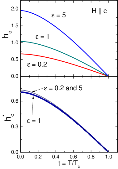
Figure 1: (Color online) The upper panel: reduced upper critical fields for a prolate $\varepsilon=0.2$ and oblate $\varepsilon=5$ spheroids and s-wave order parameter. $h_{c}(t)$ is calculated solving Eq. (48), (49), (52). The HW result for $\varepsilon=1$ is shown for comparison.
The lower panel: the same result plotted using the HW normalization (102) to show that in this representation $h_{c}$ only weakly depends on the Fermi surface shape.

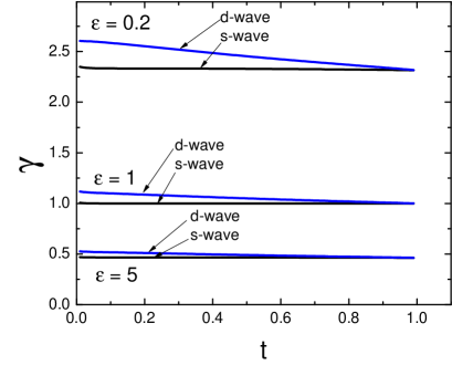
Figure 2: (Color online) Anisotropy parameter $\gamma=h_{ab}/h_{c}=H_{c2,ab}/H_{c2,c}$ calculated solving Eq. (50), (51), and (77) for s- and d-wave order parameters.

Examples of this calculation for the s-wave order parameter, $\Omega=1$, are shown in the upper panel of Fig. 1 for a prolate ellipsoid with $\varepsilon=0.2$ and for an oblate one with $\varepsilon=5$ (the latter corresponds to the ratio of spheroid semi-axes $\sqrt{5}$); the numerical procedure is outlined in Appendix C. The plotted $h_{c}(t)$ is $H_{c2,c}$ normalized on $\phi_{0}/(\hbar^{2}v_{0}^{2}/2\pi T_{c}^{2})$ with $v_{0}$ given in Eq. (47) in terms of the Fermi energy and the total density of states. For comparison, the same results are shown in the lower panel of Fig. 1 in the traditional HW normalization

$$h_{c}^{*}=\frac{H_{c2,c}(T)}{T_{c}H_{c2,c}^{\prime}(T_{c})}=\frac{h_{c}(t)}{h_{c}^{\prime}(1)}\,.$$ (102)

It is seen, therefore, that for one-band s-wave materials, although the actual values of $h_{c}(0)$ vary, the curves of $H_{c2,c}(T)$ have qualitatively similar shapes for different Fermi surfaces.

VII.2 $\bm{\gamma(t)}$

To solve Eq. (50) for $\bm{H}\parallel\bm{a}$, we need

$$\mu_{b} = \frac{v_{x}^{2}+\gamma^{2}v_{z}^{2}}{v^{2}_{0}}$$ (103)

$$= D^{2/3}(\varepsilon)\frac{\sin^{2}\theta\cos^{2}\varphi+\gamma^{2}\varepsilon^{2}\cos^{2}\theta}{\Gamma(\theta,\varepsilon)}.\qquad$$

The anisotropy parameter $\gamma$ is calculated with the help of Eq. (50), (51) and shown in Fig. 2. It is worth observing that for the s-wave case, $\gamma$ depends on the Fermi surface shape but is temperature independent.

One can see that $\gamma=1$ for a Fermi sphere with $\varepsilon=1$, as is should be. One can show that $\gamma(\varepsilon)$ behave approximately as $1/\sqrt{\varepsilon}$. In particular, we observe that for oblate Fermi spheroids, $\gamma<1$, i.e., $H_{c2,ab}<H_{c2,c}$.

VII.3 d-wave on a one-band ellipsoid

For this case $\Omega=\Omega_{0}\cos 2\varphi$ and one can verify that the condition $\langle\Omega^{2}\rangle=1$ yields $\Omega_{0}^{2}=2$, the same value for any Fermi spheroid. Eq. (48) then can be solved numerically with the results shown in Fig. 3 for values of $\varepsilon$ given in the caption. The anisotropy parameter for d-wave is shown in Fig. 2; unlike s-wave, it decreases on warming.

It is worth observing that for a fixed $\varepsilon$, $h_{c}(t)$ for s- and d-wave order parameters are the same. This is because the Fermi surface average in Eq. (48) involves $(1/2)\int_{0}^{\pi}\sin\theta d\theta$ for the s-wave whereas for the d-wave we have $(1/4\pi)\int_{0}^{\pi}\sin\theta d\theta\int_{0}^{2\pi}2\cos^{2}2\phi\,d\phi$ which has the same value as for the s-case.

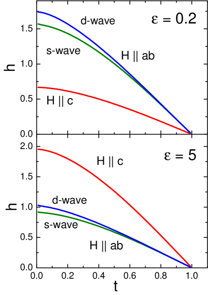
Figure 3: (Color online) Reduced fields $h(t)$ for two spheroids, $\varepsilon=0.2,5$. For $\bm{H}\parallel c$, s- and d-curves coincide, as explained in the text.

VII.4 Order parameter modulated along $\bm{k_{z}}$

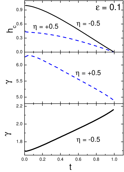
Figure 4: (Color online) The reduced field $h_{c}(t)$ is shown in the upper panel for a spheroid with $\varepsilon=0.1$ and the order parameter (104) with $a=1$ and $\eta=\pm 0.5$. Two lower panels show the anisotropy parameter $\gamma(t)$.

The gap function suggested by the ARPES data for Ba_0.6K_0.4Fe₂As₂ has a general form:Xu

$$\Delta=\Delta_{0}(1+\eta\cos k_{z}a)\,.$$ (104)

This order parameter varies along the Fermi surface with changing $k_{z}$; it does not have zeros if $|\eta|<1$. Depending on the sign of $\eta$, it has maximum or minimum at the “equator” $k_{z}=0$.

To apply this dependence for Fermi spheroids, we write:

$$k_{z}^{2}=k_{F}^{2}\cos^{2}\theta=\frac{2m_{ab}E_{F}\cos^{2}\theta}{\hbar^{2}\Gamma(\varepsilon,\theta)}\,,$$ (105)

where $k_{F}$ is taken from Eq. (134). Since $m_{\parallel}=2E_{F}/v_{\parallel}^{2}$ and $v_{\parallel}=v_{0}D^{1/3}$, we obtain

$$k_{z}a=\frac{2E_{F}a\cos\theta}{\hbar v_{0}D^{1/3}(\varepsilon)\sqrt{\Gamma(\varepsilon,\theta)}}\,.$$ (106)

We now choose the length scale

$$a=\frac{\hbar v_{0}}{2E_{F}}\,,$$ (107)

so that

$$k_{z}a=\frac{\cos\theta}{D^{1/3}(\varepsilon)\sqrt{\Gamma(\varepsilon,\theta)}}\,.$$ (108)

Note that in the isotropic case, the length $a=a_{0}/(3\pi^{2})^{1/3}$ with $a_{0}$ being the interparticle spacing (the unit cell size).

To adopt the order parameter (104) for our formalism we define

$$\Omega^{2}=\frac{(1+\eta\cos(k_{z}a))^{2}}{\langle(1+\eta\cos(k_{z}a))^{2}\rangle}\,,$$ (109)

as to satisfy the normalization $\langle\Omega^{2}\rangle=1$ (the average in the denominator is calculated according to Eq. (140)).

Numerical evaluation of $h_{c}(t)$ for parameters given in the caption of Fig. 4 result in a curve qualitatively similar to that of HW (the upper panel), however, the anisotropy parameter decreases on warming for $\eta>0$ as shown in the middle panel. It is quite remarkable that changing the sign of $\eta$, i.e., going from order parameters with a maximum at the Fermi surface “equator” $k_{z}=0$ ($\eta>0$) to ones with a minimum ($\eta<0$), not only changes the temperature dependence of $\gamma$ to the opposite, but affects its absolute values as well (for positive $\eta$, the anisotropy parameter is noticeably larger than for $\eta<0$ for other parameters kept the same).

One can readily evaluate how the anisotropy of the London penetration depth $\Lambda$, $\gamma_{\Lambda}=\Lambda_{c}/\Lambda_{ab}$, changes with temperature for $\eta=-0.5$ (for which the $H_{c2}$ anisotropy is shown in the lowest panel of Fig. 4). To this end we note that the GL theory requires the same values of these two anisotropies at $T_{c}$, so that $\gamma_{\Lambda}(T_{c})=\gamma(T_{c})\approx 2.17$ according to Fig. 4. As $T\to 0$, $\gamma_{\Lambda}^{2}(0)\to\langle v_{x}^{2}\rangle/\langle v_{z}^{2}\rangle$ (in the clean limit, the order parameter does not enter the anisotropy of the London depth).RC ; gamma-model ; RPP The calculation of these averages is straightforward for a spheroid with $\varepsilon=0.1$: $\gamma_{\Lambda}(0)\approx 3.38$. Thus, the $\Lambda$-anisotropy decreases on warming, unlike $H_{c2}$-anisotropy. This qualitative behavior of the $\Lambda$-anisotropy is, in fact, seen in experiments on Ba(Fe_1-xCo_x)₂As₂, (Ba_1-xK_x)Fe₂As₂, and NdFeAs(O_1-xF_x).Prozetal

In Fig. 5 we demonstrate that the effect of $\gamma$ increasing on warming remains if the Fermi surface changes from a prolate spheroid with $\varepsilon=0.1$ to a sphere $\varepsilon=1$ and to oblate spheroid with $\varepsilon=5$. In particular, these features challenge the common belief that temperature dependence of the anisotropy parameter is always related to a multi-band situations.

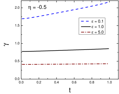
Figure 5: (Color online) The anisotropy parameter $\gamma(t)$ for three different Fermi surfaces $\varepsilon=0.1,1,5$ and the order parameter of the form (104) with $\eta=-0.5$.

We note in concluding this Section that other possible anisotropic order parameters can be treated within our scheme in a similar manner.

VIII Two-band results

To apply the theory developed for two-band materials one first should map actual band structure upon two spheroids, the procedure we demonstrate in some detail on the well-studied MgB₂. When calculating parameters $\mu_{c}$ (and $\mu_{b}$) needed in this mapping for each band, one should bear in mind that in the two-band situation we have:

$$\mu_{c,\alpha}=\left[\frac{D(\varepsilon_{\alpha})}{n_{\alpha}}\right]^{2/3}\,\frac{\sin^{2}\theta}{\Gamma(\theta,\varepsilon_{\alpha})}\,,$$ (110)

see Appendix C.

VIII.1 MgB₂

We take this example to demonstrate that our procedure yields $H_{c2,c}(T)$ and the anisotropy $\gamma(T)$ in agreement with existing data (see, e.g. Refs. Lyard, ; Budko, ) and with calculations of Refs. MMK, ; DS, ; Palistrant, . We stress that our calculations of $H_{c2}$ are done with the same set of coupling parameters as those used for the zero-field properties of this material as described in Ref. gamma-model, .

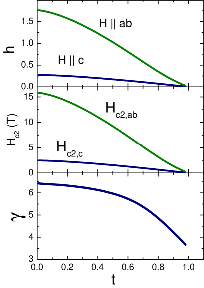
Figure 6: (Color online) The upper panel: reduced upper critical fields of clean MgB₂. $h_{c}(t)$ is calculated solving Eq. (76), (77) for two spheroids with ellipticity parameters $\varepsilon_{1}=0.02867$ (a strongly prolate spheroid for nearly 2D $\sigma$ band) and $\varepsilon_{2}=1.273$ (for a 3D $\pi$ band) evaluated with the help of two-bands Fermi velocities from the band structure calculations of Ref. Bel, . The reduced couplings $\lambda_{\alpha\beta}$ are evaluated on the basis of microscopic calculations of Ref. Golubov, as described in the text. The middle panel: the same for the fields in common units; $H_{c2,c}(0)\approx 2.8\,$T and $H_{c2,ab}(0)\approx 16\,$T. The lower panel: the anisotropy parameter $\gamma=h_{ab}/h_{c}=H_{c2,ab}/H_{c2,c}$ calculated solving Eq. (76), (77) with $\mu_{c}$ replaced by $\mu_{b}(\gamma)$.

The four Fermi sheets of MgB₂ can be grouped in two effective bands with nearly constant zero-field gaps for each group.Choi The two effective bands are mapped here upon two ellipsoids.MMK We describe this procedure in some detail.

We take the following data from the band structure calculations:Golubov the relative densities of states of our model are $n_{1}\approx 0.42$ and $n_{2}\approx 0.58$ for $\sigma$ and $\pi$ bands, respectively.Bel ; Choi The band calculationsBel provide also the averages over separate Fermi sheets: $\langle v_{a}^{2}\rangle_{1}=23$, $\langle v_{c}^{2}\rangle_{1}=0.5$, and $\langle v_{a}^{2}\rangle_{2}=33.2$, $\langle v_{c}^{2}\rangle_{2}=42.2\times 10^{14}\,$cm²/s².

To map this system onto two Fermi ellipsoids, we note that the averages over spheroids are given by

$$\langle v_{x}^{2}\rangle = \frac{v_{\parallel}^{2}}{2D(\varepsilon)}\int_{0}^{1}\frac{du(1-u^{2})}{\Gamma^{3/2}(\varepsilon)\Gamma_{1}^{1/2}(\varepsilon)}\,,$$ (111)

$$\langle v_{z}^{2}\rangle = \frac{v_{\parallel}^{2}\varepsilon^{2}}{D(\varepsilon)}\int_{0}^{1}\frac{du\,u^{2}}{\Gamma^{3/2}(\varepsilon)\Gamma_{1}^{1/2}(\varepsilon)}\,,\quad\qquad$$ (112)

where $u=\cos\theta$. The integrals here can be expressed in terms of Elliptic Integrals, alternatively they can be evaluated numerically. Forming the ratio $\langle v_{x}^{2}\rangle/\langle v_{z}^{2}\rangle$ we obtain an equation which can be solved for $\varepsilon$. This gives $\varepsilon_{1}=0.02867$ and $\varepsilon_{2}=1.273$. For a given $\varepsilon$ and, e.g., $\langle v_{z}^{2}\rangle\equiv\langle v_{c}^{2}\rangle$, we obtain $v_{ab}^{2}$ for two ellipsoids: $v_{ab,1}^{2}=0.6019\times 10^{14}$ and $v_{ab,2}^{2}=1.436\times 10^{16}$ (cm/s)². Next, we write:

$$\frac{1}{v_{0}^{3}} = \frac{\pi^{2}\hbar^{3}(N_{1}+N_{2})}{2E_{F}^{2}}=\frac{1}{v_{01}^{3}}+\frac{1}{v_{02}^{3}}$$ (113)

$$= \frac{D(\varepsilon_{1})}{v_{\parallel,1}^{3}}+\frac{D(\varepsilon_{2})}{v_{\parallel,2}^{3}}$$

where Eq. (100) has been used; this gives $v_{0}^{2}=3.867\times 10^{14}$ (cm/s)², the constant used in the field normalization.

To obtain normalized coupling constants $\lambda_{\alpha\beta}=V_{\alpha\beta}/V_{0}$ we use the effective values (calculated including Coulomb repulsion) which in our notation read: $N_{1}V_{11}=0.807$, $N_{2}V_{22}=0.276$, $N_{1}V_{21}=0.118$, $N_{2}V_{12}=0.086$.Golubov Using Eq. (64) one evaluates $1/V_{0}N(0)=1.211$, and obtains the normalized coupling

$$\lambda_{11}=\frac{V_{11}}{V_{0}}=\frac{N_{1}V_{11}}{N(0)V_{0}}\frac{1}{n_{1}}\approx 2.328\,.$$ (114)

Similarly, we find $\lambda_{22}=0.5765$, $\lambda_{12}=\lambda_{21}=0.340$. With these input parameters we have solved Eqs. (76), (77) for $h_{c}(t)$. The result is shown in the upper panel of Fig. 6.

Given $h_{c}(t)$, we rewrite the same equations where $\mu_{c}$ is replaced with $\mu_{b}(\gamma)$ and solve them for $\gamma(t)$. The latter is shown in the lower panel of Fig. 6.

Hence, the calculation gives $h_{c}(0)\approx 0.292$. We now use the relation (78) between the dimensionless $h_{c}$ and physical $H_{c2,c}$, where $T_{c}=39.5\,$K and $v_{0}$ has been estimated above, to obtain $H_{c2,c}(0)\approx 2.8\,$T, the value close to the observed.Budko ; Lyard The general behavior of $H_{c2,c}(T)$ is close to that of HW, the fact confirmed by experiment. It should be mentioned that our result is close to the calculations of Miranovic et al,MMK Dahm and Schopohl,DS and Palistrant.Palistrant We, however, do not reproduce the calculated $H_{c2,c}(T)$ with changing curvature and a substantial upturn at low $T$’s of Ref. Gurevich2, .

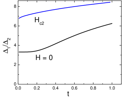
Figure 7: (Color online) The ratio $\Delta_{1}/\Delta_{2}$ of two order parameters of MgB₂ at $H_{c2,c}$ and at zero field calculated with the same coupling constants.

The general formula for the gaps ratio at $H_{c2}$ is given in Eq. (81). Figure 7 shows this ratio as a function of temperature at $H_{c2,c}$. For comparison we show the gaps ratio in zero field calculated with the help of the same coupling constants.gamma-model It is instructive to note that the gaps ratio at $H_{c2}$ exceeds the zero-field value at all temperatures, that can be interpreted as a stronger suppression of the small gap by the magnetic field than that of the large one at the leading $\sigma$ band. At first sight, one would expect the two ratios to coincide as $T\to T_{c}$, which our results clearly do not show. Such an expectation, however, would not be justified: even when $H_{c2}\to 0$, the superconductor in the mixed state differs from the uniform state by an extra magnetic field suppression of the order parameter.

One often finds in literature the statement that a small gap in MgB₂ is substantially or even completely suppressed by a large enough field. This would correspond to a substantial increase of $\Delta_{1}/\Delta_{2}$ or even divergence of this ratio at some field under $H_{c2}$. Our result, however, shows that even at $H_{c2}$ the gaps ratio is finite and of the same order at all $T$’s. We conclude that the full suppression of the small gap does not happen at any field $H\leq H_{c2}$. On the other hand, assuming (as was done in Ref. MMK, ) that the gap ratio at $H_{c2}$ is the same as that calculated in zero field, is also incorrect.

VIII.2 $\bm{\lambda_{11}\sim\lambda_{22}\ll|\lambda_{12}|}$

This case is close to theoretical models of pnictides in which the interband coupling is assumed dominant. We consider here a limiting situation $\lambda_{11}=\lambda_{22}=0$ to simplify the algebra. Indeed, for the two field directions we have:

$$(\ln t)^{2} - 4h_{c}^{2}\,{\cal I}_{1}(\mu_{c})\,{\cal I}_{2}(\mu_{c})=0\,,\qquad$$ (115)

$$(\ln t)^{2} - 4h_{c}^{2}\,{\cal I}_{1}(\mu_{b})\,{\cal I}_{2}(\mu_{b})=0\,.\qquad$$ (116)

The first equation here can be solved for $h_{c}(t)$. Since $\mu_{b}$ depends on $\gamma$, the second gives an equation for $\gamma(t)$. The latter can also be written in a different form if one subtracts Eq. (115) from (116):

$${\cal I}_{1}(\mu_{c})\,{\cal I}_{2}(\mu_{c})={\cal I}_{1}(\mu_{b})\,{\cal I}_{2}(\mu_{b})\,.$$ (117)

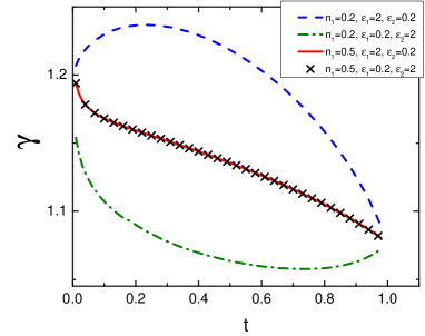
Figure 8: (Color online) The field $h_{c}(t)$ (the upper panel) and the anisotropy parameter $\gamma(t)$ (the lower panel) for the order parameter of the form $\Delta=\Delta_{0}(1+\eta\cos k_{z}a)$ . The parameters chosen are: $\varepsilon_{1}=\varepsilon_{2}=0.1$, $n_{1}=0.5$, $a=1$, for three sets of $\eta$’s given in the figure.

Fig. 8 shows numerical solution for $\gamma(t)$ for a few representative parameter sets. It is worth noting the particularly informative feature of Fig. 8: it shows that the anisotropy $\gamma(t)$ is not necessarily a monotonic function of temperature. We note that numerical calculations of $\gamma(t)$ showing an extremum at $0<t<1$ are quite robust.

VIII.2.1 $\bm{\Delta_{1}/\Delta_{2}}$

The general result for the gaps ratio (81) gives for $\lambda_{11}=\lambda_{22}=0$:

$$\frac{\Delta_{1}}{\Delta_{2}}=\frac{\ln t}{2n_{1}\lambda_{12}h_{c}{\cal I}_{1}}\,.$$ (118)

Near $T_{c}$ we use $\cal I$’s of Eq. (53) and $h_{c}$ from Eq. (115) to obtain:

$$\frac{\Delta_{1}}{\Delta_{2}}\Big{|}_{T_{c}}=\frac{1}{n_{1}\lambda_{12}}\sqrt{\frac{\langle\Omega^{2}\mu_{c}\rangle_{2}}{\langle\Omega^{2}\mu_{c}\rangle_{1}}}=\sqrt{\frac{n_{2}\langle\Omega^{2}\mu_{c}\rangle_{2}}{n_{1}\langle\Omega^{2}\mu_{c}\rangle_{1}}}\,,$$ (119)

since for $\lambda_{11}=\lambda_{22}=0$, the normalized $\lambda_{12}^{2}=1/n_{1}n_{2}$. As $T\to 0$, we can keep only the leading term $\sim\ln t$ in $\cal I$ of Eq. (56):

$$\frac{\Delta_{1}}{\Delta_{2}}\Big{|}_{T=0}=\sqrt{\frac{n_{2}}{n_{1}}}\,.$$ (120)

It is instructive to note that the last relation in the form $n_{1}\Delta_{1}^{2}=n_{2}\Delta_{2}^{2}$ at $T=0$ suggests the equipartition of condensation energy between the bands (provided the only non-zero coupling is $\lambda_{12}$).

VIII.2.2 Two bands with $\bm{\Delta(k_{z})}$

This example is of interest because it may have implications for understanding the behavior of $H_{c2}(T)$ and, in particular, its anisotropy in Fe-based materials. In Fig. 9 we show $h_{c}(t)$ and $\gamma(t)$ for two nearly cylindrical bands with order parameters modulated along $k_{z}$ according to Eq. (104). Modulations are characterized by $\eta_{1}=\eta_{2}=-0.2$; other parameters are given in the caption. The main feature worth paying attention to is the anisotropy $\gamma(t)$ which is increasing on warming for negative $\eta$’s.

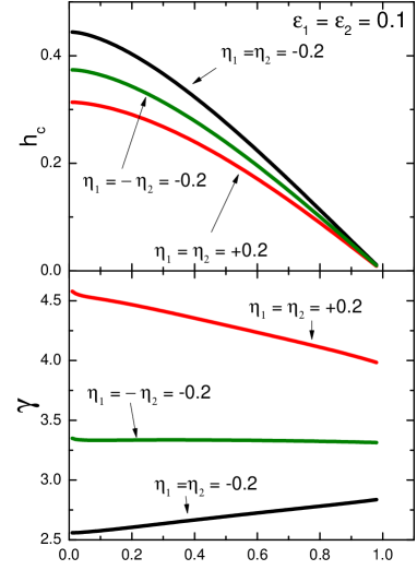
Figure 9: (Color online) The field $h_{c}(t)$ (the upper panel) and the anisotropy parameter $\gamma(t)$ (the lower panel) for the order parameter of the form $\Delta=\Delta_{0}(1+\eta\cos k_{z}a)$ . The parameters chosen are: $\varepsilon_{1}=\varepsilon_{2}=0.1$, $n_{1}=0.5$, $a=1$, for three sets of $\eta$’s given in the figure.

It is worth noticing that experimental anisotropy of Fe-based materials behaves qualitatively similar to that shown by the lowest curve in the lower panel of Fig. 9.Budko-Canfield We, however, do not have enough information to fix the necessary parameters for realistic calculations (one needs partial densities of states, Fermi surfaces characterized separately for relevant bands for evaluating the geometric parameters $\varepsilon$’s, and the order parameters $\Delta(\bm{k}_{F})$). Hence, we take our results as having a generic qualitative value. In particular, among various possibilities we have considered, only the order parameters of the form $\Delta=\Delta_{0}(1+\eta\cos k_{z}a)$ combined with dominant role of the inter-band coupling yield the $\gamma(t)$ increasing on warming similar to what is seen experimentally.

IX Summary and Conclusions

The upper critical field $H_{c2}$ and its anisotropy are among the easiest properties to examin when a new superconductor is discovered. This work provides a relatively straightforward scheme for evaluating the orbital $H_{c2}(T)$ and its anisotropy $\gamma(T)$ for single and two band uniaxial materials. We reproduce here the main points of our approach.

The input parameters for two band materials are (i) the coupling matrix $V_{\alpha\beta}$ (or the normalized couplings $\lambda_{\alpha\beta}$ and $T_{c}$), (ii) the symmetries of the order parameter on two bands given as $\Omega_{\beta}(\theta,\phi)$, $\beta$ is the band index, with the normalization (3), and (iii) the characteristics of electron systems (Fermi surfaces, averages of squared Fermi velocities, DOS’).

The equation to solve for the reduced upper critical field $h_{c}(t)$ parallel to the $c$ crystal axis of a two-band clean uniaxial material reads:

$$(\ln t)^{2} - 2h_{c}(n_{1}\lambda_{11}{\cal I}_{1}+n_{2}\lambda_{22}{\cal I}_{2})\ln t$$ (121)

$$+ 4h_{c}^{2}(n_{1}\lambda_{11}+n_{2}\lambda_{22}-1){\cal I}_{1}{\cal I}_{2}=0\,,\qquad$$

$${\cal I}_{\beta} = \int_{0}^{\infty}ds\,s\ln\tanh(st)\Big{\langle}\Omega^{2}\mu_{c}e^{-\mu_{c}s^{2}h_{c}}\Big{\rangle}_{\beta}\,,\qquad$$ (122)

where $\mu_{c}$ is given by Eq. (49) for the corresponding band, and $\Omega$’s describe the order parameter symmetries. After $h_{c}(t)$ is found, one solves Eq. (121), in which $\mu_{c}$ is replaced by $\mu_{b}(\gamma)$ of Eq. (51), for $\gamma(t)$. The one-band case is obtained by setting $n_{2}=0,n_{1}=1$ and $\lambda_{11}=1$. The case of two s-wave bands corresponds to $\Omega_{1}=\Omega_{2}=1$.

Because $H_{c2}$ is determined by equations containing only integrals over the Fermi surface, it is insensitive to fine details of the Fermi surface shape. Therefore, one can replace actual Fermi surfaces with ellipsoids (or with spheroids, for uniaxial materials). Given the averages of the squared Fermi velocities over each band, one establishes the geometry of corresponding rotational ellipsoids (the squared ratio of semi-axes, $\varepsilon$). This procedure is described in Section VIII.A on the well-studied example of MgB₂.

One numerically solves Eqs. (121), (122) by employing any of available packages (such as Mathematica) able to find roots of nonlinear equations and to do multiple integrals. The scheme can also be applied to the case of two bands with order parameters of different symmetries.

By design, our method is applicable for clean materials with a moderate $H_{c2}(0)$; paramagnetic limiting effects are out of the scope of this work.Gurevich2 The method differs from those previously employed by not involving explicit coordinate dependent $\Delta_{1,2}$ and minimization relative to the vortex lattice structures in calculating $H_{c2}(T)$.Scharn-Klemm ; Rieck ; MMK ; DS The main feature of the two-band derivation is that the linearized GL equation (70) is assumed to hold at $H_{c2}(T)$ at any $T$, the ansatz proven correct by satisfying the self-consistency equation of the theory. The method is tested on the well-studied example of MgB₂ where it shows a satisfactory agreement with data and with other calculations.

Our main results are as follows:

1. We find that in clean one-band s-wave materials, the $T$ dependence of the anisotropy $\gamma$ cannot be caused by the Fermi surface anisotropy (however, the paramagnetic limit, which is out of the scope of this paper, may suppress $\gamma$ at low $T$’s and cause $\gamma(T)$ to increase on warming).

2. For other than s-wave symmetry, $\gamma$ depends on temperature even for one-band materials. This dependence is pronounced for open Fermi surfaces as well as for order parameters depending on $k_{z}$. Thus, the common belief that the temperature dependence of the anisotropy parameter is always related to multi-band situations is incorrect.

3. Our scheme of calculating $H_{c2}$ for two-band materials does not utilize any assumptions about the field and temperature dependences of the order parameters $\Delta_{\alpha}$ in two bands.MMK In fact, the gaps ratio is calculated self-consistenly and in general turns out temperature dependent. Although both $\Delta_{1}$ and $\Delta_{2}$ turn zero at $H_{c2}(T)$, their ratio is finite and in the examples examined is larger than at zero field.

4. The case of exclusively inter-band coupling is discussed, that might be relevant while interpreting data on $H_{c2}$ and its anisotropy in Fe-based compounds.

5. For order parameters of the form $\Delta=\Delta_{0}(1+\eta\cos k_{z}a)$ (one of the candidates suggested for pnictides), the anisotropy parameter $\gamma(t)$ depends on the sign of $\eta$ (or $\eta$’s for two-bands). In particular, $\gamma(T)$ increases on warming in a nearly linear fashion (as for pnictides) for both $\eta$’s negative.

Appendix A Different form of the one-band equation for ${\bm{H}_{\bm{c}\bm{2}}}$

Both sides of Eq. (48) diverge logarithmically when $t\to 0$, so that these divergences, in fact, cancel out. However, in numerical work this cancellation may not always be exact which may cause the numerical solutions to become unreliable in this limit. Here, we provide an alternative form of this equation free of this shortcoming.

To this end, consider an identity:

$$\ln t = \left\langle\Omega^{2}2h_{c}\mu\int_{0}^{\infty}ds\,s\ln(st)\,e^{-\mu h_{c}s^{2}}\right\rangle$$ (123)

$$+ \frac{\bm{C}+\left\langle\ln(\Omega^{2}h_{c}\mu)\right\rangle}{2}\,,$$

which is verified by direct integration. We now combine it with Eq. (48):

$$\frac{\bm{C}+\left\langle\Omega^{2}\ln(h_{c}\mu)\right\rangle}{4h_{c}}$$

$$=\int_{0}^{\infty}ds\,s\ln\frac{\tanh(st)}{st}\left\langle\Omega^{2}\mu e^{-\mu h_{c}s^{2}}\right\rangle.\qquad$$ (124)

As $t\to 0$, the integral on the RHS goes to zero, and we immediately obtain the result (57) for $h_{c}(0)$.

Appendix B ${\bm{T}_{\bm{c}}}$ as a function of ${\bm{\lambda}_{\bm{\alpha}\bm{\beta}}}$

This question had been discussed, e.g., in Ref. gamma-model, ). Since our notation of normalized $\lambda_{\alpha\beta}$ differs from that in the literature, we provide here corresponding relations. The s-wave self consistency equation for $H=0$,

$$\Delta_{\nu}=2\pi T\sum_{\mu,\omega}N_{\mu}V_{\nu\mu}f_{\mu}(\omega)\,,\qquad$$ (125)

gives near $T_{c}$ where $f_{\mu}=\Delta_{\mu}/\hbar\omega$:

$$\Delta_{\nu}=\sum_{\mu}n_{\mu}N(0)V_{0}\lambda_{\nu\mu}\Delta_{\mu}\sum_{\omega}^{\omega_{D}}\frac{2\pi T}{\hbar\omega}\,,\qquad$$ (126)

where $V_{0}$ is to be defined. We choose it so that

$$\frac{1}{N(0)V_{0}}=\sum_{\omega}^{\omega_{D}}\frac{2\pi T}{\hbar\omega}=\ln\frac{2\hbar\omega_{D}}{1.76T_{c}}\,,\qquad$$ (127)

or, which is the same, $1.76T_{c}=2\hbar\omega_{D}e^{-1/N(0)V_{0}}$. We then obtain a linear and homogeneous system of equations $\Delta_{\nu}=\sum_{\mu}n_{\mu}\lambda_{\nu\mu}\Delta_{\mu}$, zero determinant of which gives Eq. (66).

For other than s-wave order parameters on two bands, we take the coupling potential in the form (84) and the order parameters as in Eq. (85), We then obtain the self-consistency equation $\Psi_{\nu}=2\pi T\sum_{\mu,\omega}N_{\mu}V^{(0)}_{\nu\mu}\langle\Omega_{\mu}f_{\mu}(\omega)\rangle$. We now denote $\lambda_{\nu\mu}=V^{(0)}_{\nu\mu}/V_{0}$, Eq. (87), and recall that $f_{\mu}=\Omega_{\mu}\Psi_{\mu}/\hbar\omega$ near $T_{c}$. This gives $\Psi_{\nu}=\sum_{\mu}n_{\mu}\lambda_{\nu\mu}\Psi_{\mu}$, i.e. the same system of equations as above for the s-wave case and the same zero-determinant condition (66) albeit with renormalized couplings (87).

Appendix C $\bm{\mu}_{\bm{c}}$ for the two-band case

By definition, $\mu_{c,\beta}\propto v^{2}_{ab,\beta}/v_{0}^{2}$ with $v_{0}$ given in Eq. (47). For $v_{ab,\beta}$ we have two relations: one with the Fermi energy, $m_{ab,\beta}v_{ab,\beta}^{2}=2E_{F}$, and the other in terms of the band DOS, Eq. (95):

$$N_{\beta}=\frac{m^{2}_{ab,\beta}v_{ab,\beta}}{2\pi^{2}\hbar^{3}}\,D(\varepsilon_{\beta})\,,\qquad\beta=1,2\,.$$ (128)

One excludes $m_{ab,\beta}$ from these two relations to obtain:

$$v_{ab,\beta}^{3}=\frac{2E_{F}^{2}}{\pi^{2}\hbar^{3}N_{\beta}}\,.$$ (129)

Hence, we have:

$$\mu_{c,\beta}=\frac{v_{ab,\beta}^{2}}{v_{0}^{2}}=\left[\frac{D(\varepsilon_{\beta})}{n_{\beta}}\right]^{2/3}\,,$$ (130)

a clear generalization of Eq. (100) for the one-band spheroid. This gives Eq. (110) used in the text.

Appendix D Open Fermi Surface

The theory employed above is designed to model Fermi surfaces closed within the first Brillouin zone. Here we consider an example of the Fermi surface which crosses the zone boundary, i.e. it is open. Perhaps, the simplest shape to consider is a rotational hyperboloid which is a property of the carriers energy of the form:

$$E(\bm{k})=\hbar^{2}\left(\dfrac{k_{x}^{2}+k_{y}^{2}}{2m_{ab}}-\dfrac{k_{z}^{2}}{2m_{c}}\right)\,.$$ (131)

A schematic picture is shown in Fig.10.

Figure 10: (Color online) The cross-section $k_{y}=0$ of an open Fermi hyperboloid. $k_{z,BZ}$ is the zone boundary in the $\hat{c}$ direction. Tilted straight lines correspond to $E=0$, whereas the hyperbola shows the Fermi surface.

In spherical coordinates $(k,\theta,\phi)$ we have

$$E(\bm{k}) = \dfrac{\hbar^{2}k^{2}}{2m_{ab}}\left(\sin^{2}\theta-\dfrac{m_{ab}}{m_{c}}\cos^{2}\theta\right)=\dfrac{\hbar^{2}k^{2}}{2m_{ab}}\Gamma_{2}(\theta),\qquad$$

$$\Gamma_{2} = \sin^{2}\theta-\epsilon\cos^{2}\theta\,,\quad\epsilon=m_{ab}/m_{c}\,.$$ (132)

It is seen from the figure that in the first quadrant of the plane $k_{x},k_{z}$, the Fermi surface is situated at $\theta>\theta_{m}>\tan^{-1}\sqrt{\epsilon}$, i.e., everywhere at the Fermi surface $\Gamma_{2}>0$.

The angle $\theta_{m}$ corresponds to the crossing of the Fermi hyperboloid with the zone boundary $k_{z,BZ}=2\pi/c$ where $c$ is the unit cell size along the $\hat{c}$ direction:

$$\tan^{2}\theta_{m}=\epsilon+\frac{m_{ab}c^{2}E_{F}}{2\pi^{2}\hbar^{2}}=\epsilon+\alpha\,.$$ (133)

The parameter $\alpha=k^{2}_{F}(\pi/2)/k_{z,BZ}^{2}\,$ in most situations of interest is less than unity ($k_{F}(\pi/2)$ is the radius of the hyperboloid neck).

The Fermi momentum is given by

$$k_{F}^{2}(\theta)=\frac{2m_{ab}E_{F}}{\hbar^{2}\Gamma_{2}(\theta)}\,.$$ (134)

The Fermi velocity is $\bm{v}(\bm{k})=\bm{\nabla}_{\bm{k}}E(\bm{k})_{\bm{k}_{F}}$:

$$v_{x}=\dfrac{v_{ab}\sin\theta\cos\phi}{\sqrt{\Gamma_{2}(\theta)}},\,\,\,v_{y} = \dfrac{v_{ab}\sin\theta\sin\phi}{\sqrt{\Gamma_{2}(\theta)}},$$

$$v_{z}=\epsilon\dfrac{v_{ab}\cos\theta}{\sqrt{\Gamma_{2}(\theta)}},\qquad v_{ab} = \sqrt{2E_{F}/m_{\parallel}}\,.\qquad$$ (135)

Futher, we have for $v=(v_{x}^{2}+v_{y}^{2}+v_{z}^{2})^{1/2}$:

$$v=v_{ab}\sqrt{\dfrac{\sin^{2}\theta+\epsilon^{2}\cos^{2}\theta}{\sin^{2}\theta-\epsilon\cos^{2}\theta}}=v_{ab}\sqrt{\dfrac{\Gamma_{1}(\theta)}{\Gamma_{2}(\theta)}}\,.$$ (136)

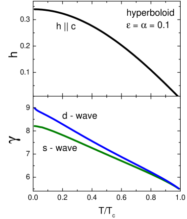
Figure 11: (Color online) The upper panel: $h_{c}(t)$ for Fermi hyperboloid with $\epsilon=\alpha=0.1$. The lower panel: the anisotropy $\gamma(t)$ for the same parameters of the Fermi hyperboloid.

The density of states $N(0)$ is defined by the integral of Eq. (94), which can be written as an integral over the solid angle $d\Omega=\sin\theta\;d\theta\,d\phi$:

$$N(0)=\dfrac{m^{2}_{ab}v_{ab}}{2\pi^{2}\hbar^{3}}\int\dfrac{d\Omega}{4\pi\sqrt{\Gamma_{2}(\theta)\Gamma_{1}(\theta)}}\,,$$ (137)

where the integration over $\theta$ is extended from $\theta_{m}$ to $\pi-\theta_{m}$. The Fermi surface average of a function $A(\theta,\phi)$ is

$$\langle A\rangle = \frac{1}{D}\displaystyle\int\dfrac{d\Omega\,A(\theta,\phi)}{4\pi\sqrt{\Gamma_{2}(\theta)\Gamma_{1}(\theta)}}\,,\qquad\qquad$$ (138)

$$D = \int\dfrac{d\Omega}{4\pi\sqrt{\Gamma_{2}(\theta,\epsilon)\Gamma_{1}(\theta,\epsilon)}}\,.$$ (139)

For $A$ depending only on $\theta$, one can employ $u=\cos\theta$:

$$\langle A\rangle=\frac{1}{D(\epsilon)}\int_{0}^{u_{m}}\frac{du\,A(u)}{\sqrt{\Gamma_{2}(u,\epsilon)\Gamma_{1}(u,\epsilon)}}\,,\qquad\qquad$$ (140)

$$\Gamma_{2}=1-(\epsilon+1)u^{2}\,,\qquad\Gamma_{1}=1+(\epsilon^{2}-1)u^{2}\,.\qquad$$ (141)

where the upper limit is $u_{m}=\cos\theta_{m}=1/\sqrt{1+\epsilon+\alpha}$. In particular, one obtains:

$$D(\epsilon,\alpha)=\frac{F(\tan^{-1}\sqrt{(1+\epsilon)/\alpha},1-\epsilon)}{\sqrt{1+\epsilon}}\qquad$$ (142)

where $F$ is an Incomplete Elliptic Integral of the first kind.

As for ellipsoids, the relation between $v_{ab}$ and $v_{0}$ defined in Eq. (47) for a one-band situation holds:

$$v_{ab}^{3}=D\,v_{0}^{3}\,,$$ (143)

however, with a different $D$.

For $\bm{H}\parallel\hat{c}$, the relevant electron orbits are circular, as for spheres and rotational ellipsoids, and we do not expect qualitative deviations from the latter. Fig.LABEL:hc-hyperb shows $h_{c}(t)$ calculated with the help of Eqs. (48) and (49) for both s- and d-wave order parameters. We note that the anisotropy parameter shown in this figure is suppressed substantially on warming.

Numerical evaluation of the anisotropy shows that $\gamma(t)$ decreases on warming, Fig. 11. Reduction of the anisotropy on warming is substantial for a single band open Fermi surface, an interesting observation given the common belief that the temperature dependence of anisotropy is a multi-band property. We also note that this reduction is stronger than that of open Fermi surfaces.

References

- (1) E. Helfand and N.R. Werthamer, Phys. Rev. 147, 288 (1966). Another part of this work published as a separate paper by N.R. Werthamer, E. Helfand, and P.C. Hohenberg, Phys. Rev. 147, 295 (1966), WHH, is devoted to spin paramagnetism and spin-orbit effects. Dealing with orbital effects we refer to HW, although quite often WHH is cited when the intention is to mention the seminal HW calculation of the orbital .
- (2) P. Miranović, K. Machida and V. G. Kogan, J. Phys. Soc. of Japan 72, No.2, 221 (2003).
- (3) T. Dahm and N. Schopohl, Phys. Rev. Lett. 91, 017001 (2003).
- (4) Y-M. Xu, Y-B. Huang, X-Y. Cui, E. Razzoli, M. Radovic, M. Shi, G-F. Chen, P. Zheng, N-L.Wang, C-L. Zhang, P-C. Dai, J-P. Hu, Z.Wang and H. Ding, Nature Physics, 7, 198 (2011).
- (5) L. N. Bulaevskii, Phys. Zh. Eksp. Teor. Fiz. 65, 1278 (1973); Sov. Phys. JETP. 38, 634 (1974).
- (6) D.W. Youngner and R.A. Klemm, Phys. Rev., 21, 3890 (1980).
- (7) A. Gurevich, Phys. Rev., 67, 184515 (2003).
- (8) A. Gurevich, Phys. Rev., 82, 184504 (2010).
- (9) M. E. Palistrant, I. D. Cebotaru, V. A. Ursu, arXiv: 0811.0897; M. Palistrant, A. Surdua, V. Ursu and P. Petrenko, A. Sidorenko, Low Temp. Phys. 37, No.6, 451 (2011).
- (10) S. Haas and K. Maki, Phys. Rev. B65, 020502(R) (2001).
- (11) T. Kita and M. Arai, Phys. Rev. B70, 224522 (2004).
- (12) V.G. Kogan, S.L. Bud’ko, Physica C, Superconductivity 385, 131 (2003).
- (13) N. Ni, M. E. Tillman, J.-Q. Yan, A. Kracher, S. T. Hannahs, S. L. Bud ko, and P. C. Canfield, Phys. Rev. B78, 214515 (2008).
- (14) A. Gurevich, Rep. Prog. Phys. 74, 124501 (2011).
- (15) J. L. Zhang, L. Jiao, Y. Chen, H. Q. Yuan, Front. Phys, 6(4), 463 (2011,); arXiv:1201.2548.
- (16) M. Sigrist and K. Ueda, Rev. Mod. Phys. 63, 239 (1991).
- (17) R. Joynt and L. Taillefer, Rev. Mod. Phys. 74, 235 (2002).
- (18) C. T. Rieck and K. Scharnberg, Physica B 163, 670 (1990).
- (19) G. Eilenberger, Z. Phys. 214, 195 (1968).
- (20) V. G. Kogan, Phys. Rev. B66, 020509 (2002).
- (21) D. Markowitz and L. P. Kadanoff, Phys. Rev. 131, 363 (1963).
- (22) L. P. Gor’kov and T. K. Melik-Barkhudarov, Soviet Phys. JETP, 18, 1031 (1964).
- (23) D. R. Tilley, Proc. Phys. Soc. London, 85, 1177 (1965).
- (24) T. Terashima, M. Kimata, H. Satsukawa, A. Harada, K. Hazama, S. Uji, H. Harima, Gen-Fu Chen, Jian-Lin Luo, and Nan-Lin Wang, Journ. Phys. Soc. Jap. 78, 063702 (2009).
- (25) H. Q. Yuan, J. Singleton, F. F. Balakirev, S. A. Baily, G. F. Chen, J. L. Luo, and N. L. Wang, Nature, 457, 565 (2009).
- (26) Hechang Lei and C. Petrovic, EPL, 95, 57006 (2011).
- (27) S. Kittaka, Y. Aoki, T. Sakakibara, A. Sakai, S. Nakatsuji, Y. Tsutsumi, M. Ichioka, and K. Machida, arXiv:1111.5388
- (28) Zhao-Sheng Wang, Hui-Qian Luo, Cong Ren and Hai-Hu Wen, Phys. Rev. B, 78, 140501R (2008).
- (29) Chun-Hong Li, Bing Shen, Fei Han, Xiyu Zhu, and Hai-Hu Wen, Phys. Rev. B83, 184521 (2011).
- (30) M. Shahbazi, X. L. Wang, S. R. Ghorbani, S. X. Dou, and K. Y. Choi, Appl. Phys. Lett. 100, 102601 (2012).
- (31) V.G. Kogan, Phys. Rev. B, 26, 88 (1982).
- (32) L.P. Gor’kov, Zh. Exp. Teor. Fiz. 37, 833 (1959); Sov. Phys. JETP, 10, 593 (1960).
- (33) L. D. Landau and E. M. Lifshitz, Classical Theory of Fields,…
- (34) P. M. Morse and H. Feshbach Methods of Theoretical Physics, McGraw-Hill, 1953; v.1, Section 1.3.
- (35) V. G. Kogan and J. Schmalian, Phys. Rev. B 83, 054515 (2011).
- (36) A. A. Shanenko, M. Milosevic, F. Peeters, Phys. Rev. Lett. 106, 047005 (2011).
- (37) M. E. Zhitomirsky and V.-H. Dao, Phys. Rev. B69, 054508 (2004).
- (38) It is instructive to note that the zero- value of the ratio of coordinate dependent order parameters at the upper critical field is the same as at zero-field and .gamma-model ; KS
- (39) V. G. Kogan, C. Martin, R. Prozorov, Phys. Rev. B80, 014507 (2009).
- (40) R. Prozorov and V. G. Kogan, Rep. Prog. Phys. 74, 124505 (2011).
- (41) R. Prozorov, M. A. Tanatar, R. T. Gordon, C. Martin, H. Kim, V. G. Kogan, N. Ni, M. E. Tillman, S. L. Bud ko, P. C. Canfield, Physica C, Superconductivity, 469, 582 (2009).
- (42) L. Lyard et al., Phys. Rev. B 66, 180502 (2002).
- (43) H. J. Choi, D. Roundy, Hong Sun, M. L. Cohen, S. G. Louie, Nature, London, 418, 758 (2002).
- (44) K.D. Belashchenko, M. van Schilfgaarde, and V.P. Antropov, Phys. Rev. B 64, 092503 (2001).
- (45) A.A. Golubov, J. Kortus, O.V. Dolgov, O. Jepsen, Y. Kong, O.K. Andersen, B.J. Gibson, K. Ahn, and R.K. Kremer, J. Phys.: Condens. Matter 14, 1353 (2002).
- (46) K. Scharnberg and R. A. Klemm, Phys. Rev. B 22, 5233 (1980).
- (47) P. J. Hirschfeld, M. M. Korshunov and I. I. Mazin, Rep. Prog. Phys. 74, 124508 (2011).