Dynamics of an Intruder in Dense Granular Fluids

Abstract

We investigate the dynamics of an intruder pulled by a constant force in a dense two-dimensional granular fluid by means of event-driven molecular dynamics simulations. In a first step, we show how a propagating momentum front develops and compactifies the system when reflected by the boundaries. To be closer to recent experiments candelier2010journey ; candelier2009creep , we then add a frictional force acting on each particle, proportional to the particle’s velocity. We show how to implement frictional motion in an event-driven simulation. This allows us to carry out extensive numerical simulations aiming at the dependence of the intruder’s velocity on packing fraction and pulling force. We identify a linear relation for small and a nonlinear regime for high pulling forces and investigate the dependence of these regimes on granular temperature.

1 Introduction

The response of an intruder to a pulling force is a rather versatile tool to study the local nonequilibrium dynamics in various complex fluids, such as glasses hastings2003depinning , colloids habdas04 ; gazuz09 and granular media candelier2010journey ; candelier2009creep ; zik92 ; sarracino2010irreversible . The measured force-velocity relations reveal striking nonlinear behaviour close to the glass and/or jamming transition. In the early experiments on colloids evidence was given for a threshold force even in the fluid regime, whereas mode-coupling theory predicts such behaviour only in the glassy phase. In the experiment of Ref. candelier2010journey ; candelier2009creep two transitions are observed: the first one, called fluidization, separates a regime of continuous to intermittent motion of the intruder. It occurs below the jamming point (the second transition) and depends on the applied pulling force. Experimentally it is observed even for the smallest pulling force with the possibility of a dynamic transition inherent to the vibrated granular fluid for zero applied force. In Ref. reichhardt2010 , the dynamics of an intruder was simulated near the jamming point. One result of this study are velocity-force relations which are linear for packing fraction, $\eta\leq 0.833$ and become nonlinear for $\eta$ still closer to the jamming point.

In contrast to reichhardt2010 , we discuss a stochastically driven system, describing a fluidized granular state – similar to the experimental setup in candelier2010journey ; candelier2009creep . A recent mode-coupling theory kranz2010 predicts that such a “thermalized” granular fluid undergoes a glass transition at a packing fraction below the jamming point. This transition is different from both, the jamming transition at zero temperature and the glass transition for either Newtonian or Brownian dynamics.

In this paper we use event driven simulations to analyze the dynamics of an intruder in a two-dimensional system of hard disks close to the glass transition. We compute force-velocity correlations in the linear and nonlinear regime, extract the mobility for the linear regime and discuss scaling for the nonlinear regime. Moreover we discuss the dependence on the granular temperature.

2 Model

We consider a bidisperse system of $N$ hard disks in an area $A$. Particles’ positions and velocities are denoted by $\{\mathbf{r}_{i}\}_{i=1}^{N}$ and $\{\mathbf{v}_{i}\}_{i=1}^{N}$. The size ratio $R_{s}/R_{b}=4:5$ of small to big particles is chosen as in the experiments of Refs. candelier2010journey ; candelier2009creep . The mass ratio follows from the disk like shape of the particles as $m_{s}/m_{b}=16/25$. The intruder with position $\mathbf{r}_{0}$ and velocity $\mathbf{v}_{0}$ is chosen twice as large as the small particles, $R_{0}=2R_{s}$ and $m_{0}=4m_{s}$.

The particles collide inelastically so that in each collision energy is dissipated while momentum is conserved. The simplest model ignores rotational degrees of freedom, allowing for normal restitution only. The collision rules for two colliding particles (say ₁ and ₂) is given in terms of their relative velocity $\mathbf{g}:=\mathbf{v}_{1}-\mathbf{v}_{2}$

$$(\mathbf{g}\cdot\mathbf{n})^{\prime}=-\epsilon(\mathbf{g}\cdot\mathbf{n}).$$ (1)

where $\epsilon$ is the coefficient of restitution and $\mathbf{n}$ denotes the unit vector $\mathbf{n}:=(\mathbf{r}_{1}-\mathbf{r}_{2})/|\mathbf{r}_{1}-\mathbf{r}_{2}|$ at contact.

In between collisions the particles perform Brownian motion, due to friction with a surrounding medium or with the bottom plate. We model this by a frictional force in the equation of motion: $\mathbf{F}_{\mathrm{fr}}=-\gamma m\mathbf{v}$. For all finite values of the friction coefficient $\gamma$, momentum is lost, whereas for $\gamma=0$, the total momentum is conserved.

Inelastic collisions give rise to a loss of energy $\propto\frac{1-\epsilon^{2}}{2}T$, where $T$ denotes the granular temperature $T=\frac{1}{2N}\sum_{i=1}^{N}m_{i}v_{i}^{2}$. To balance this dissipation the entire system is driven stochastically (like an air-fluidized bed oger-1996 ; abate-2006 ; abate-07 or a vibrating bottom plate urbach-2005 ; reis-2006 ; reis-2007 ) by instantaneous kicks. The momentum of the $i$-th particle $\mathbf{p}_{i}(t)$ is changed according to

$$\mathbf{p}_{i}^{\prime}(t)=\mathbf{p}_{i}(t)+p_{\mathrm{dr}}\bm{\xi}_{i}(t)$$ (2)

with $\langle\xi_{i}^{\alpha}(t)\xi_{j}^{\beta}(t^{\prime})\rangle=\delta_{ij}\delta_{\alpha\beta}\delta(t-t^{\prime})$ and zero mean $\langle\xi_{i}^{\alpha}(t)\rangle=0$, and $\alpha=x,z$ denoting the cartesian components. In the frictional case, $\gamma\neq 0$, we kick single particles, whereas for the frictionless case, $\gamma=0$, we kick neighbouring particles with equal and opposite momenta in order to conserve the total momentum locally fiege-2009 .

We want to investigate the dynamics of a tagged particle under the action of a deterministic pulling force $\mathbf{F}$. This so called intruder with position $\mathbf{r}_{0}$ and velocity $\mathbf{v}_{0}$ is subject to systematic kicks

$$\mathbf{p}_{0}^{\prime}(t)=\mathbf{p}_{0}(t)+\mathbf{F}\Delta t$$ (3)

mimicking a constant force acting on the intruder. The frequency of these systematic kicks $(\Delta t)^{-1}$ is chosen 4 orders of magnitude higher than the frequency of the stochastic driving and the collision frequency (see below). The systematic force does work on the system, injecting momentum and energy.

Combining inelastic collisions, stochastic driving, pulling force and friction, we arrive at the following equation of motion

$$\dot{p}_{i}^{\alpha}(t)=-\gamma p_{i}^{\alpha}(t)+F\delta_{\alpha,x}\delta_{i,0}+\left.\frac{\mathrm{d}p_{i}^{\alpha}}{\mathrm{d}t}\right|_{\mathrm{dr}}+\left.\frac{\mathrm{d}p_{i}^{\alpha}}{\mathrm{d}t}\right|_{\mathrm{coll}}.$$ (4)

We aim to prepare the granular fluid without pulling force to be under stationary conditions. This can be achieved by balancing energy dissipation due to friction and inelastic collisions by the stochastic driving. Without external forcing the mean velocity of the particles vanishes, so that the granular temperature, $T=\frac{1}{2N}\sum_{i=1}^{N}m_{i}v_{i}^{2}$, is just the average kinetic energy of the particles. Its time rate of change can be deduced from Eq. 4 by multiplying with ${p}_{i}^{\alpha}(t)$ yielding

$$\frac{1}{2}\frac{d}{dt}\left({p}_{i}^{\alpha}\right)^{2}(t)=-\gamma(p_{i}^{\alpha}(t))^{2}+\frac{1}{2}\left.\frac{\mathrm{d}}{\mathrm{d}t}\right|_{\mathrm{dr}}(p_{i}^{\alpha})^{2}+\frac{1}{2}\left.\frac{\mathrm{d}}{\mathrm{d}t}\right|_{\mathrm{coll}}(p_{i}^{\alpha})^{2}.$$ (5)

The explicit calculation of the time derivations on the rhs are beyond the scope of this paper but may be found elsewhere aspelmeier2001free ; kranz2011 . The time rate of change of the granular temperature then reads as follows:

$$\frac{\mathrm{d}T}{\mathrm{d}t}=-2\gamma T-\omega_{E}\frac{1-\epsilon^{2}}{2}T+f_{\mathrm{dr}}\frac{p_{\mathrm{dr}}^{2}}{2m_{\mathrm{eff}}},$$ (6)

where the effective mass is given by $m_{\mathrm{eff}}=\frac{m_{s}m_{b}}{m_{s}+m_{b}}$. For simplicity, we choose the driving frequency $f_{\mathrm{dr}}$ equal to the Enskog frequency $\omega_{E}$ boon1991molecular and measure length and mass in units, such that $R_{s}=1$ and $m_{s}=1$. In the stationary state, $\frac{\mathrm{d}T}{\mathrm{d}t}=0$, the amplitude of the stochastic driving is given by:

$$\frac{p_{\mathrm{dr}}^{2}}{2m_{\mathrm{eff}}}=\frac{2\gamma T}{\omega_{E}}+\frac{1-\epsilon^{2}}{2}T.$$ (7)

We prepare our system in a stationary state with $T=1$, yielding a numerical value for $p_{\mathrm{dr}}$ depending on $\gamma$, $\omega_{E}$ and $\epsilon$.

3 Simulations

3.1 Implementation as event-driven simulation

In order to apply an event-driven algorithm to the dynamics, as described by Eq. (4), we need to generalize the code to account for damping ($\gamma\neq 0$). As usual, events include collisions of particles, wall collisions, subbox-wall collisions and (discrete) driving events (kicks). Standard event driven algorithms calculate the time of an upcoming event and advance all particles to that time under the assumption that the particle motion is ballistic. Hence, in between events, the velocities do not change. The condition for a collision is $R_{i}+R_{j}=\left|\mathbf{r}_{i}(t^{\bullet})-\mathbf{r}_{j}(t^{\bullet})\right|$, i.e., the difference in the particles’ trajectories at the collision time $t^{\bullet}$ must be equal to the sum of their radii. Plugging in the trajectories subject to ballistic motion $\mathbf{r}_{i,j}(t^{\bullet})=\mathbf{r}_{i,j}(t_{0})+\mathbf{v}_{i,j}(t_{0})(t^{\bullet}-t_{0})$, one finds a quadratic equation, that must have a positive solution for $(t^{\bullet}-t_{0})$ if and only if a collision will occur alder-1959 ; Lubachevsky-1991 .

In our case, the velocities decrease as $\mathbf{v}_{i,j}(t^{\star})=\mathbf{v}_{i,j}(t_{0})\exp(-\gamma(t^{\star}-t_{0}))$. Integration results in

$$\mathbf{r}_{i,j}(t^{\star})=\mathbf{r}_{i,j}(t_{0})+\mathbf{v}_{i,j}(t_{0})\frac{1-e^{-\gamma(t^{\star}-t_{0})}}{\gamma}.$$ (8)

Inserting this into the condition for a collision, we find a similar condition for a collision except that $(t^{\bullet}-t_{0})$ is replaced by $\frac{1-e^{-\gamma(t^{\star}-t_{0})}}{\gamma}$, which is monotonically increasing in $(t^{\star}-t_{0})$. Since our (ballistic) event-driven code calculates $(t^{\bullet}-t_{0})$ we only have to replace the collision time by

$$t^{\star}-t_{0}=-\frac{1}{\gamma}\log\left(1-\gamma\cdot(t^{\bullet}-t_{0})\right).$$ (9)

Hence, collisions will occur at the same place and in the same order but at a different time and with different particles’ velocities, provided the place of the collision is within reach of the particle. In detail, the maximum distance a particle is able to travel is limited because of the friction slowing the particle down. The maximal distance is given by $\mathbf{r}_{i}^{max}=\lim_{t^{\star}\rightarrow\infty}\mathbf{r}_{i}(t^{\star})=\mathbf{r}_{i}(t_{0})+\mathbf{v}_{i}(t_{0})/\gamma>\mathbf{r}_{i}(t^{\bullet})$ that must be larger than the distance to the place at which the event will take place. Hence, $(\mathbf{r}_{i}(t^{\bullet})-\mathbf{r}_{i}(t_{0}))<\mathbf{v}_{i}(t_{0})/\gamma$ or $(t^{\bullet}-t_{0})<1/\gamma$. This is consistent with Eq. (9) which requires
$\log\left(1-\gamma\cdot(t^{\bullet}-t_{0})\right)$ to be negative for a positive collision time. Advancing a particle to a different type of event ( e.g. kicks) is done in the same way.

Changing an existing event-driven simulation in the way discussed enables us to simulate systems of hard disks and spheres subject to friction almost as fast as without friction. The systematic force on the intruder as described in Eq. 3 is implemented as frequent kicks on the intruder. In order to avoid an inelastic collapse, i.e., a infinite number of collisions in a finite time interval, we use the same method as described in fiege-2009 to circumvent it.

3.2 Equilibration and data aquisition

For packing fractions up to $\eta=0.8$ we used the same data sets from gholami2011slow as initial conditions. For even denser systems, we used a compactified system acquired as described in section 4.1.

The data shown in section 4.2 were obtained by first equilibrating 100 different configurations and then switching on the force on the intruder. The final velocity of the intruder was measured after stationarity was attained. The time to reach a stationary state depends on the packing fraction, the restitution coefficient and the applied force on the intruder. A typical trajectory and its corresponding fluctuating velocity for the largest packing fraction $\eta=0.8$ and force $F=100000$ is shown the inset of Fig. 4. The intruder moves approximately $3R_{0}$ in $x$-direction before fluctuating around its stationary average velocity.

4 Results

The time rate of change of the total momentum $\mathbf{P}=\frac{1}{N}\sum_{i}m_{i}\mathbf{v}_{i}$ follows from Eq. (4):

$$\dot{P}^{\alpha}(t)=-\gamma P^{\alpha}(t)+\frac{F}{N}\delta_{\alpha,x}$$ (10)

which is solved by

$$P^{\alpha}(t)=P^{\alpha}(0)e^{-\gamma t}+\delta_{\alpha,x}\frac{F}{\gamma N}(1-e^{-\gamma t})$$ (11)

Here we have used that the collisions as well as the random driving conserve momentum. In the frictional case with $\gamma\neq 0$, the total momentum goes to a constant, $P_{x}=F/(N\gamma)$, whereas for the frictionless case with $\gamma=0$, the momentum grows linearly with time, $P_{x}=Ft/N$. In the following we shall mainly discuss the first case, because the frictional model is closer to experiment. However, the frictionless case allows us to study the propagation of momentum in an inelastic fluid jabeen2010universal ; gomez2011shock .

4.1 Frictionless state ( $\gamma=0$ )

To that end, we consider a system with aspect ratio $A=5:1$, $N=5000$ and fixed walls, which reflect the particles elastically. Momentum is conserved on average except for the pulling force which constantly feeds (small) momenta into the system, which are propagated by collisions away from the source into all of the available area. Below the jamming transition momentum transport is given by ballistic motion of particles as well as by collisions. If the intruder starts at the left hand side of the system and is pulled by the external force, then only particles in the neighbourhood of the intruder will feel the local momentum input for short times. The momentum given to the intruder is distributed among the particles in front (i.e. in the direction of the pulling force) of the intruder. Again, these particles distribute their momenta by collisions as well as by ballistic transport. A front of particles carrying the momentum fed into the system by the intruder is formed (see Fig. 1 top), propagates through the system (see Fig. 1 center) and ultimately collides with the hard wall (see figure 1 bottom). At this instant the momentum is reflected by the wall and many particles end up in a highly compactified state with a packing fraction $\eta\approx 0.839$.

To analyze the momentum wave quantitatively, we plot $P_{x}$ averaged over $z$ in Fig. 2. The propagation front is well defined, its center of mass moves with velocity $V_{\mathrm{cm}}=16.51$ and it broadens with time such that it’s width increases linearly with time, $\Delta=V_{\mathrm{br}}t$ (with $V_{\mathrm{br}}=10.89$). Both velocities increase with pulling force, while their ratio is approximately constant. Hence the observed propagation front cannot be identified with linear sound but is presumably a shockwave in agreement with the observations of Ref. gomez2011shock .

\psfrag{y}{$z$}\psfrag{x}{$x$}\includegraphics[width=216.81pt]{vel_field2.eps}

Figure 1: Momentum transport with $\gamma=0$ and hard walls. A vector denoting the particle’s velocity is assigned to each particle’s position. ($T=0.1$, $\epsilon=0.9$, $F=500$, $\eta=0.8$, $t=2.6$, $6.3$, $8.5$)

\psfrag{t20}{$t=1.3125$}\psfrag{t60}{$t=3.8125$}\psfrag{t100}{$t=6.3125$}\psfrag{px}{$P^{x}$}\psfrag{x}{$x$}\includegraphics[width=216.81pt]{transport_0.eps}

Figure 2: Propagation of momentum wave; total momentum for 3 different times, in dimensionless units; (parameters as in Fig. 1).

4.2 Force-velocity relation ( $\gamma\neq 0$ )

In the following, we consider a system with $N=20000$ grains, subject to friction ($\gamma=1$) with hard walls in the $z$-direction and periodic boundary conditions in the $x$-direction, allowing for a stationary current. We analyze the steady state motion of the intruder for small and large forces as a function of packing fraction for $T=1$ and subsequently compare these results to the same system with $T=0.04$.

4.2.1 Linear Regime: Mobility of the intruder

For a small pulling force we expect a linear relation between the velocity of the intruder and the force:

$$v_{I}=\mu F,$$ (12)

defining the mobility $\mu$ of the intruder.

\psfrag{F}{$F$}\psfrag{v}{$v$}\psfrag{030}{$\eta=0.3$}\psfrag{050}{$\eta=0.5$}\psfrag{060}{$\eta=0.6$}\psfrag{070}{$\eta=0.7$}\psfrag{0725}{$\eta=0.725$}\psfrag{075}{$\eta=0.75$}\psfrag{0775}{$\eta=0.775$}\psfrag{080}{$\eta=0.8$}\includegraphics[width=216.81pt]{eps07dat.eps}

Figure 3: Velocity versus pulling force for packing fractions $0.3\leq\eta\leq 0.8$, parameters chosen: $\gamma=1,\epsilon=0.7$ and aspect ratio $A=1:2$.

In Fig. (3) we plot the velocity of the intruder versus force and indeed do observe a linear regime for small pulling force. From the slope we extract the mobility which is shown in Fig. (4).

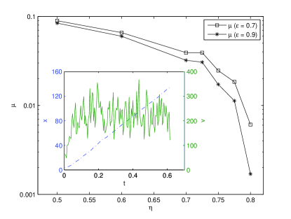
Figure 4: Mobility as a function of volume fraction for $\epsilon=0.9$ (stars) and $\epsilon=0.7$ (squares). Inset: Typical time dependence of the $x$ position and $x$ velocity of the intruder for $\epsilon=0.9$, $F=100000$ and $\eta=0.8$.

The breakdown of the mobility when the glass transition is approached is clearly visible for both investigated $\epsilon$. The more inelastic system with $\epsilon=0.7$ shows increased mobilities as compared to $\epsilon=0.9$. Since the particles are more “sticky”, they tend to stay closer after a collision than in the elastic limit, i.e., stronger density fluctuations are inherent to systems with stronger inelasticity. This enlarges the accessible space for the intruder compared to the system with $\epsilon=0.9$, increasing its average velocity. Moreover, the momentum of the intruder in the direction of the pulling force is reduced due to collisions with other particles in front. In the center of mass frame, the intruder is reflected backwards. For the more inelastic system this kind of backscattering is less effective (see Eq. 1), so that the velocity in the direction of the force and hence the mobility is larger for the more inelastic system.

4.2.2 Nonlinear regime

As the pulling force is increased, deviations from linear behaviour are expected and observed. To investigate these systematically we have applied forces in the range $1\leq F\leq 10^{5}$ and show our data in a scaling plot in Fig. (5). Scaling velocities by $v_{\mathrm{dr}}=p_{\mathrm{dr}}/m_{\mathrm{eff}}$ and forces by $v_{\mathrm{dr}}^{2}\cdot\eta^{1/2}$ collapses the data for large forces. The velocity of the intruder scales algebraically with the pulling force, according to $v_{I}\propto F^{\beta}$, $\beta=0.55$.

\psfrag{x}{$\propto F^{\beta}$}\psfrag{F}[cc]{$F/(v_{\mathrm{dr}}^{2}\cdot\eta^{1/2})$}\psfrag{v}[l]{$v/v_{\mathrm{dr}}$}\psfrag{030}[r]{$\eta=0.3$}\psfrag{050}[r]{$\eta=0.5$}\psfrag{060}[r]{$\eta=0.6$}\psfrag{070}[r]{$\eta=0.7$}\psfrag{0725}[r]{$\eta=0.725$}\psfrag{075}[r]{$\eta=0.75$}\psfrag{0775}[r]{$\eta=0.775$}\psfrag{080}[r]{$\eta=0.8$}\psfrag{xb}[r]{$F^{\beta}$}\includegraphics[width=216.81pt]{eps09collabs11.eps}

Figure 5: Velocity-force relation for all pulling forces, $\epsilon=0.9$.

The crossover between the linear and the algebraic regime is accompanied by range of forces in which the intruder velocity increases superlinearly with the applied force. This is observed at high packing fractions only, see Fig. 3. We conjecture that this shear thinning is due to the formation of vortices which can only be formed at high packing fractions, where momentum is conveyed almost instantaneously as the disks are very close to each other. For low packing fractions, the distance of neighbouring particles is too large for the formation of vortices because the damping $\gamma$ dissipates most of the momentum.

4.2.3 Temperature dependence

The crossover from linear to nonlinear response depends on the thermal velocity, $v_{\mathrm{th}} \simeq\sqrt{2T/m_{0}}\approx 0.7$. For small packing fractions, this crossover actually occurs at $v_{\mathrm{th}}$ as can be seen e.g. in Fig. 3 for the smallest packing fractions. Decreasing the temperature is expected to shrink the linear regime also for higher densities. Hence we try to explore the force velocity relation in the same system but with smaller thermal velocity. Here we choose $T=0.04$. For low pulling forces, we expect the mobility to be larger than in the case $T=1$ since the decreased thermal motion does not disturb the intruder travelling through the almost resting surrounding disks. For high forces, we expect the intruder velocity to not depend on the temperature, since in this case, the intruder’s velocity is at least one order of magnitude higher than the thermal velocity (see Fig. 5).

These expectations are indeed born out by the data. We plot the force velocity relation for packing fractions $\eta=0.6$ and $0.775$ for both temperatures in Fig. 6. For high pulling forces $F\geq 10^{3}$, the intruder velocities for low and high temperature collapse for both packing fractions as expected. For $\eta=0.6$ and $T=0.04$, the crossover from the linear regime to the nonlinear regime is shifted to smaller forces. For $\eta=0.775$ and $T=0.04$, the linear regime is not even detectable. The crossover is shifted by roughly two decades. To explore the linear regime would require forces as small as $F=10^{-2}$, at which the average intruder velocity would be too small to be detectable.

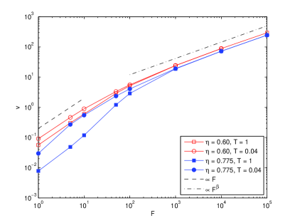
Figure 6: Velocity-force relation for strong pulling forces at different temperatures and $\epsilon=0.9$.

5 Conclusion and Outlook

We have generalised an event-driven algorithm to include friction. As a first application, we have studied the dynamics of an intruder pulled by an external force. In contrast to previous simulations reichhardt2010 , we consider a fluidized granular medium, which is expected to undergo a glass transition at a packing fraction below random close packing kranz2010 . We do indeed find a dramatic decrease of the mobility around $\eta=0.8$, in agreement with previous simulations without pulling force and consistent with a glass transition. For large pulling force, the data can be collapsed by scaling, following a power law dependence $v_{I}\propto F^{\beta}$ with $\beta=0.55$.

In the frictionless case the pulling force generates a momentum wave propagating through the sample and thereby compactifying it. We plan to investigate momentum transport in more detail in the future. Furthermore the generalised event driven algorithm will be useful more generally in the context of frictional granular matter fluidized by air or water flow. Work along these lines is in progress.

- (1) R. Candelier, O. Dauchot, Physical Review E 81(1), 011304 (2010)
- (2) R. Candelier, O. Dauchot, Physical review letters 103(12), 128001 (2009)
- (3) M. Hastings, C. Olson Reichhardt, C. Reichhardt, Physical review letters 90(9), 98302 (2003)
- (4) A. Habdas, D. Schaar, A. Levitt, E. Weeks, EPL (Europhysics Letters) 67, 477 (2004)
- (5) I. Gazuz, A. Puertas, T. Voigtmann, M. Fuchs, Physical review letters 102(24), 248302 (2009)
- (6) O. Zik, J. Stavans, Y. Rabin, EPL (Europhysics Letters) 17(4), 315 (1992)
- (7) A. Sarracino, D. Villamaina, G. Gradenigo, A. Puglisi, EPL (Europhysics Letters) 92, 34001 (2010)
- (8) C. Reichhardt, C. Reichhardt, Physical Review E 82(5), 051306 (2010)
- (9) W. Kranz, M. Sperl, A. Zippelius, Physical review letters 104(22), 225701 (2010)
- (10) L. Oger, C. Annic, D. Bideau, R. Dai, S. Savage, Journal of statistical physics 82(3), 1047 (1996)
- (11) A. Abate, D. Durian, Physical Review E 74(3), 031308 (2006)
- (12) A. Abate, D. Durian, Physical Review E 76(2), 021306 (2007)
- (13) J. Olafsen, J. Urbach, Physical review letters 95(9), 98002 (2005)
- (14) P. Reis, R. Ingale, M. Shattuck, Physical review letters 96(25), 258001 (2006)
- (15) P. Reis, R. Ingale, M. Shattuck, Physical review letters 98(18), 188301 (2007)
- (16) A. Fiege, T. Aspelmeier, A. Zippelius, Physical review letters 102(9), 98001 (2009)
- (17) T. Aspelmeier, M. Huthmann, A. Zippelius, in Granular Gases, Lecture Notes in Physics, vol. 564, ed. by T. Pöschel, S. Luding (Springer Berlin / Heidelberg, 2001), pp. 31–58
- (18) W.T. Kranz, Dense granular fluids and the granular glass transition. Ph.D. thesis, Georg-August-Universität Göttingen (2011)
- (19) J. Boon, S. Yip, Molecular hydrodynamics (Dover Pubns, 1991)
- (20) B. Alder, T. Wainwright, The Journal of Chemical Physics 31, 459 (1959)
- (21) B. Lubachevsky, Journal of Computational Physics 94(2), 255 (1991)
- (22) I. Gholami, A. Fiege, A. Zippelius, Physical Review E 84(3), 031305 (2011)
- (23) Z. Jabeen, R. Rajesh, P. Ray, EPL (Europhysics Letters) 89, 34001 (2010)
- (24) L. Gomez, A. Turner, M. van Hecke, V. Vitelli, in APS Meeting Abstracts, vol. 1 (2011), vol. 1, p. 13007