Optimality Bounds for a Variational Relaxation of the Image Partitioning Problem

Abstract

We consider a variational convex relaxation of a class of optimal partitioning and multiclass labeling problems, which has recently proven quite successful and can be seen as a continuous analogue of Linear Programming (LP) relaxation methods for finite-dimensional problems. While for the latter case several optimality bounds are known, to our knowledge no such bounds exist in the continuous setting. We provide such a bound by analyzing a probabilistic rounding method, showing that it is possible to obtain an integral solution of the original partitioning problem from a solution of the relaxed problem with an a priori upper bound on the objective, ensuring the quality of the result from the viewpoint of optimization. The approach has a natural interpretation as an approximate, multiclass variant of the celebrated coarea formula.

1 Introduction and Background

1.1 Convex Relaxations of Partitioning Problems

In this work, we will be concerned with a class of variational problems used in image processing and analysis for formulating multiclass image partitioning problems, which are of the form

$$\inf_{u\in\mathcal{C}_{\mathcal{E}}}f(u) := \int_{\Omega}\langle u(x),s(x)\rangle dx+\int_{\Omega}d\Psi(Du)\hskip 2.5pt,$$ (1)

$$\mathcal{C}_{\mathcal{E}} := \operatorname{BV}(\Omega,\mathcal{E})$$ (2)

$$= \{u\in\operatorname{BV}(\Omega)^{l}|u(x)\in\mathcal{E}\text{$\operatorname{for}$ a.e. \leavevmode\nobreak\ }x\in\Omega\},$$ (3)

$$\mathcal{E} := \{e^{1},\ldots,e^{l}\}.$$ (4)

The labeling function $u:\Omega\rightarrow\mathbb{R}^{l}$ assigns to each point in the image domain $\Omega:=(0,1)^{d}$ a label $i\in\mathcal{I}:=\{1,\ldots,l\}$, which is represented by one of the $l$-dimensional unit vectors $e^{1},\ldots,e^{l}$. Since it is piecewise constant and therefore cannot be assumed to be differentiable, the problem is formulated as a free discontinuity problem in the space $\operatorname{BV}(\Omega,\mathcal{E})$ of functions of bounded variation; we refer to Ambrosio2000 for a general overview.

The objective function $f$ consists of a data term and a regularizer. The data term is given in terms of the $L^{1}$ function $s(x)=(s_{1}(x),\ldots,s_{l}(x))\in\mathbb{R}^{l}$, and assigns to the choice $u(x)=e^{i}$ the “penalty” $s_{i}(x)$, in the sense that

$$\int_{\Omega}\langle u(x),s(x)\rangle dx = \sum_{i=1}^{l}\int_{\Omega_{i}}s_{i}(x)dx,$$ (5)

where $\Omega_{i}:=u^{-1}(\{e^{i}\})=\{x\in\Omega|u(x)=e^{i}\}$ is the class region for label $i$, i.e., the set of points that are assigned the $i$-th label. The data term generally depends on the input data – such as color values of a recorded image, depth measurements, or other features – and promotes a good fit of the minimizer to the input data. While it is purely local, there are no further restrictions such as continuity, convexity etc., therefore it covers many interesting applications such as segmentation, multi-view reconstruction, stitching, and inpainting Paragios2006 .

1.2 Convex Regularizers

The regularizer is defined by the positively homogeneous, continuous and convex function $\Psi:\mathbb{R}^{d\times l}\rightarrow\mathbb{R}_{\geqslant 0}$ acting on the distributional derivative $Du$ of $u$, and incorporates additional prior knowledge about the “typical” appearance of the desired output. For piecewise constant $u$, it can be seen that the definition in (1) amounts to a weighted penalization of the discontinuities of $u$:

$$\int_{\Omega}d\Psi(Du)=$$ (6)

$$\quad\int_{J_{u}}\Psi(\nu_{u}(x)(u^{+}(x)-u^{-}(x))^{\top})d\mathcal{H}^{d-1}(x),$$

where $J_{u}$ is the jump set of $u$, i.e., the set of points where $u$ has well-defined right-hand and left-hand limits $u^{+}$ and $u^{-}$ and (in an infinitesimal sense) jumps between the values $u^{+}(x),u^{-}(x)\in\mathbb{R}^{l}$ across a hyperplane with normal $\nu_{u}(x)\in\mathbb{R}^{d}$, $\|\nu_{u}(x)\|_{2}=1$ (see Ambrosio2000 for the precise definitions).

A particular case is to set $\Psi=(1/\sqrt{2})\|\cdot\|_{2}$, i.e., the scaled Frobenius norm. In this case $J(u)$ is just the (scaled) total variation of $u$, and, since $u^{+}(x)$ and $u^{-}(x)$ assume values in $\mathcal{E}$ and cannot be equal on the jump set $J_{u}$, it holds that

$$J(u) = \frac{1}{\sqrt{2}}\int_{J_{u}}\|u^{+}(x)-u^{-}(x)\|_{2}d\mathcal{H}^{d-1}(x),$$ (7)

$$= \mathcal{H}^{d-1}(J_{u}).$$ (8)

Therefore, for $\Psi=(1/\sqrt{2})\|\cdot\|_{2}$ the regularizer just amounts to penalizing the total length of the interfaces between class regions as measured by the $(d-1)$-dimensional Hausdorff measure $\mathcal{H}^{d-1}$, which is known as uniform metric or Potts regularizer.

A general regularizer was proposed in Lellmann2011 , based on Chambolle2008 : Given a metric (distance) $d:\{1,\ldots,l\}^{2}\rightarrow\mathbb{R}_{\geqslant 0}$ (not to be confused with the ambient space dimension), define

$$\Psi_{d}(z=(z^{1},\ldots,z^{l})):=\sup_{v\in\mathcal{D}_{\operatorname{loc}}^{d}}\langle z,v\rangle,$$ (9)

$$\mathcal{D}_{\operatorname{loc}}^{d}:=\{\left(v^{1},\ldots,v^{l}\right)\in\mathbb{R}^{d\times l}|\ldots$$ (10)

$$\quad\|v^{i}-v^{j}\|_{2}\leqslant d(i,j)\forall i,j\in\{1,\ldots,l\},\ldots$$

$$\quad\sum_{k=1}^{l}v^{k}=0\}.$$

It was then shown that

$$\Psi_{d}(\nu(e^{j}-e^{i})^{\top}) = d(i,j),$$ (11)

therefore in view of (1.2) the corresponding regularizer is non-uniform: the boundary between the class regions $\Omega_{i}$ and $\Omega_{j}$ is penalized by its length, multiplied by the weight $d(i,j)$ depending on the labels of both regions.

However, even for the comparably simple regularizer (7), the model (1) is a (spatially continuous) combinatorial problem due to the integral nature of the constraint set $\mathcal{C}_{\mathcal{E}}$, therefore optimization is nontrivial. In the context of multiclass image partitioning, a first approach can be found in Lysaker2006 , where the problem was posed in a level set-formulation in terms of a labeling function $\phi:\Omega\rightarrow\left\{1,\ldots,l\right\}$, which is subsequently relaxed to $\mathbb{R}$. Then $\phi$ is replaced by polynomials in $\phi$, which coincide with the indicator functions $u_{i}$ for the case where $\phi$ assumes integral values. However, the numerical approach involves several nonlinearities and requires to solve a sequence of nontrivial subproblems.

In contrast, representation (1) directly suggests a more straightforward relaxation to a convex problem: replace $\mathcal{E}$ by its convex hull, which is just the unit simplex in $l$ dimensions,

$$\Delta_{l} := \operatorname{conv}\{e^{1},\ldots,e^{l}\}$$

$$= \{a\in\mathbb{R}^{l}|a\geqslant 0,\sum_{i=1}^{l}a_{i}=1\},$$

and solve the relaxed problem

$$\inf_{u\in\mathcal{C}} f(u)$$ , (13)

$$\mathcal{C} := \operatorname{BV}(\Omega,\Delta_{l})$$ (14)

$$= \{u\in\operatorname{BV}(\Omega)^{l}|u(x)\in\Delta_{l}\text{$\operatorname{\leavevmode\nobreak\ for}$ a.e.\leavevmode\nobreak\ }x\in\Omega\}\hskip 2.5pt.$$ (15)

Sparked by a series of papers Zach2008 ; Chambolle2008 ; Lellmann2009 , recently there has been much interest in problems of this form, since they – although generally nonsmooth – are convex and therefore can be solved to global optimality, e.g., using primal-dual techniques. The approach has proven useful for a wide range of applications Kolev2009 ; Goldstein2009a ; Delaunoy2009 ; Yuan2010 .

1.3 Finite-Dimensional vs. Continuous Approaches

Many of these applications have been tackled before in a finite-dimensional setting, where they can be formulated as combinatorial problems on a grid graph, and solved using combinatorial optimization methods such as $\alpha$-expansion and related integer linear programming (ILP) methods Boykov2001 ; Komodakis2007 . These methods have been shown to yield an integral labeling $u^{\prime}\in\mathcal{C}_{\mathcal{E}}$ with the a priori bound

$$f(u^{\prime}) \leqslant 2\frac{\max_{i\neq j}d(i,j)}{\min_{i\neq j}d(i,j)}f(u^{\ast}_{\mathcal{E}}),$$ (16)

where $u^{\ast}_{\mathcal{E}}$ is the (unknown) solution of the integral problem (1). They therefore permit to compute a suboptimal solution to the – originally NP-hard Boykov2001 – combinatorial problem with an upper bound on the objective. No such bound is yet available for methods based on the spatially continuous problem (13).

Despite these strong theoretical and practical results available for the finite-dimensional combinatorial energies, the function-based, spatially continuous formulation (1) has several unique advantages:

• The energy (1) is truly isotropic, in the sense that for a proper choice of $\Psi$ it is invariant under rotation of the coordinate system. Pursuing finite-dimensional “discretize-first” approaches generally introduces artifacts due to the inherent anisotropy, which can only be avoided by increasing the neighborhood size, thereby reducing sparsity and severely slowing down the graph cut-based methods.

  In contrast, properly discretizing the relaxed problem (13) and solving it as a convex problem with subsequent thresholding yields much better results without compromising sparsity (Fig. 1 and 2, Klodt2008 )

  

  

  

  

  

  

  

  

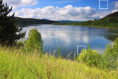
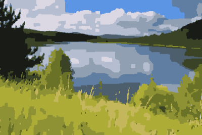
  Figure 1: Segmentation of an image into $12$ classes using a combinatorial method. Left: Input image, Right: Result obtained by solving a combinatorial discretized problem with $4$-neighborhood. The bottom row shows detailed views of the marked parts of the image. The minimizer of the combinatorial problem exhibits blocky artifacts caused by the choice of discretization.

  .

  

  

  

  

  

  

  

  

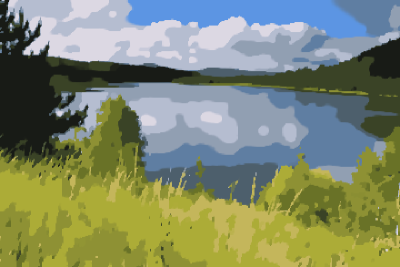
  Figure 2: Segmentation obtained by solving a finite-differences discretization of the relaxed spatially continuous problem. Left: Non-integral solution obtained as a minimizer of the discretized relaxed problem. Right: Integral labeling obtained by rounding the fractional labels in the solution of the relaxed problem to the nearest integral label. The rounded result contains almost no structural artifacts.

  This can be attributed to the fact that solving the discretized problem as a combinatorial problem in effect discards much of the information about the problem structure that is contained in the nonlinear terms of the discretized objective.

• Present combinatorial optimization methods Boykov2001 ; Komodakis2007 are inherently sequential and difficult to parallelize. On the other hand, parallelizing primal-dual methods for solving the relaxed problem (13) is straight-forward, and GPU implementations have been shown to outperform state-of-the-art graph cut methods Zach2008 .

• Analyzing the problem in a fully functional-analytic setting gives valuable insight into the problem structure, and is of theoretical interest in itself.

1.4 Optimality Bounds

However, one possible drawback of the spatially continuous approach is that the solution of the relaxed problem (13) may assume fractional values, i.e., values in $\Delta_{l}\setminus\mathcal{E}$. Therefore, in applications that require a true partition of $\Omega$, some rounding process is needed in order to generate an integral labeling $\bar{u}^{\ast}$. This may increase the objective, and lead to a suboptimal solution of the original problem (1).

The regularizer $\Psi_{d}$ as defined in (9) enjoys the property that it majorizes all other regularizers that can be written in integral form and satisfy (11). Therefore it is in a sense “optimal”, since it introduces as few fractional solutions as possible. In practice, this forces solutions of the relaxed problem to assume integral values in most points, and rounding is in practice only required in small regions.

However, the rounding step may still increase the objective and generate suboptimal integral solutions. Therefore the question arises whether this approach allows to recover “good” integral solutions of the original problem (1).

In the following, we are concerned with the question whether it is possible to obtain, using the convex relaxation (13), integral solutions with an upper bound on the objective. Specifically, we focus on inequalities of the form

$$f(\bar{u}^{\ast}) \leqslant (1+\varepsilon)f(u_{\mathcal{E}}^{\ast})$$ (17)

for some constant $\varepsilon>0$, which provide an upper bound on the objective of the rounded integral solution $\bar{u}^{\ast}$ with respect to the objective of the (unknown) optimal integral solution $u_{\mathcal{E}}^{\ast}$ of (1). Note that generally it is not possible to show that (17) holds for any $\varepsilon>0$. The reverse inequality

$$f(u_{\mathcal{E}}^{\ast})\leqslant f(\bar{u}^{\ast})$$ (18)

always holds since $\bar{u}^{\ast}\in\mathcal{C}_{\mathcal{E}}$ and $u_{\mathcal{E}}^{\ast}$ is an optimal integral solution. The specific form (17) can be attributed to the alternative interpretation

$$\frac{f(\bar{u}^{\ast})-f(u_{\mathcal{E}}^{\ast})}{f(u_{\mathcal{E}}^{\ast})} \leqslant \varepsilon,$$ (19)

which provides a bound for the relative gap to the optimal objective of the combinatorial problem. Such $\varepsilon$ can be obtained a posteriori by actually computing (or approximating) $\bar{u}^{\ast}$ and a dual feasible point: Assume that a feasible primal-dual pair $\left(u,v\right)\in\mathcal{C}\times\mathcal{D}$ is known, where $u$ approximates $u^{\ast}$, and assume that some integral feasible $\bar{u}\in\mathcal{C}_{\mathcal{E}}$ has been obtained from $u$ by a rounding process. Then the pair $\left(\bar{u},v\right)$ is feasible as well since $\mathcal{C}_{\mathcal{E}}\subseteq\mathcal{C}$, and we obtain an a posteriori optimality bound of the form (19) with respect to the optimal integral solution $u^{\ast}_{\mathcal{E}}$:

$$\frac{f(\bar{u})-f_{D}(u_{\mathcal{E}}^{\ast})}{f_{D}(u_{\mathcal{E}}^{\ast})}\leqslant\frac{f(\bar{u})-f_{D}(u_{\mathcal{E}}^{\ast})}{f_{D}(v)}\leqslant\frac{f(\bar{u})-f_{D}(v)}{f_{D}(v)}=:\varepsilon^{\prime}\hskip 2.5pt.$$ (20)

However, this requires that the the primal and dual objectives $f$ and $f_{D}$ can be accurately evaluated, and requires to compute a minimizer of the problem for the specific input data, which is generally difficult, especially in the spatially continuous formulation.

In contrast, true a priori bounds do not require knowledge of a solution and apply uniformly to all problems of a class, irrespective of the particular input. When considering rounding methods, one generally has to discriminate between

• deterministic vs. probabilistic methods, and

• spatially discrete (finite-dimensional) vs. spatially continuous methods.

Most known a priori approximation results only hold in the finite-dimensional setting, and are usually proven using graph-based pairwise formulations. In contrast, we assume an “optimize first” perspective due to the reasons outlined in the introduction. Unfortunately, the proofs for the finite-dimensional results often rely on pointwise arguments that cannot directly be transferred to the continuous setting. Deriving similar results for continuous problems therefore requires considerable additional work.

1.5 Contribution and Main Results

In this work we prove that using the regularizer (9), the a priori bound (16) can be carried over to the spatially continuous setting. Preliminary versions of these results with excerpts of the proofs have been announced as conference proceedings Lellmann2011 . We extend these results to provide the exact bound (16), and supply the full proofs.

As the main result, we show that it is possible to construct a rounding method parametrized by a parameter $\gamma\in\Gamma$, where $\Gamma$ is an appropriate parameter space:

$$R: \mathcal{C}\times\Gamma\rightarrow\mathcal{C}_{\mathcal{E}},$$ (22)

$$u\in\mathcal{C}\mapsto\bar{u}_{\gamma}:=R_{\gamma}(u)\in\mathcal{C}_{\mathcal{E}},$$

such that for a suitable probability distribution on $\Gamma$, the following theorem holds for the expectation $\mathbb{E}f(\bar{u}):=\mathbb{E}_{\gamma}f(\bar{u}_{\gamma})$:

Theorem 1.1

Let $u\in\mathcal{C}$, $s\in L^{1}(\Omega)^{l}$, $s\geqslant 0$, and let $\Psi:\mathbb{R}^{d\times l}\rightarrow\mathbb{R}_{\geqslant 0}$ be positively homogeneous, convex and continuous. Assume there exists a lower bound $\lambda_{l}>0$ such that, for $z=(z^{1},\ldots,z^{l})$,

$$\Psi(z) \geqslant \lambda_{l}\frac{1}{2}\sum_{i=1}^{l}\|z^{i}\|_{2}\hskip 10.00002pt\forall z\in\mathbb{R}^{d\times l},\sum_{i=1}^{l}z^{i}=0.$$ (23)

Moreover, assume there exists an upper bound $\lambda_{u}<\infty$ such that, for every $\nu\in\mathbb{R}^{d}satisfying\|\nu\|_{2}=1$,

$$\Psi(\nu(e^{i}-e^{j})^{\top}) \leqslant \lambda_{u}\quad\forall i,j\in\{1,\ldots,l\}\,.$$ (24)

Then Alg. 1 (see below) generates an integral labeling $\bar{u}\in\mathcal{C}_{\mathcal{E}}$ almost surely, and

$$\mathbb{E}f(\bar{u}) \leqslant 2\frac{\lambda_{u}}{\lambda_{l}}f(u).$$ (25)

Note that $\lambda_{u}\geqslant\lambda_{l}$ always holds if both are defined, since (23) implies, for $\nu$ with $\|\nu\|_{2}=1$,

$$\lambda_{u}\geqslant\Psi(\nu(e^{i}-e^{j})^{\top}) \geqslant \frac{\lambda_{l}}{2}(\|\nu\|_{2}+\|\nu\|_{2})=\lambda_{l}.$$ (26)

The proof of Thm. 1.1 (Sect. 4) is based on the work of Kleinberg and Tardos Kleinberg1999 , which is set in an LP relaxation framework. However their results are restricted in that they assume a graph-based representation and extensively rely on the finite dimensionality. In contrast, our results hold in the continuous setting without assuming a particular problem discretization.

Theorem 1.1 guarantees that – in a probabilistic sense – the rounding process may only increase the energy in a controlled way, with an upper bound depending on $\Psi$. An immediate consequence is

Corollary 1

Under the conditions of Thm. 1.1, if $u^{\ast}$ minimizes $f$ over $\mathcal{C}$, $u_{\mathcal{E}}^{\ast}$ minimizes $f$ over $\mathcal{C}_{\mathcal{E}}$, and $\bar{u}^{\ast}$ denotes the output of Alg. 1 applied to $u^{\ast}$, then

$$\mathbb{E}f\left(\bar{u}^{\ast}\right) \leqslant 2\frac{\lambda_{u}}{\lambda_{l}}f(u_{\mathcal{E}}^{\ast}).$$ (27)

Therefore the proposed approach allows to recover, from the solution $u^{\ast}$ of the convex relaxed problem (13), an approximate integral solution $\bar{u}^{\ast}$ of the nonconvex original problem (1) with an upper bound on the objective.

In particular, for the tight relaxation of the regularizer as in (9), we obtain (cf. Prop. 10)

$$\mathbb{E}f(\bar{u}^{\ast}) \leqslant 2\frac{\lambda_{u}}{\lambda_{l}}=2\frac{\max_{i\neq j}d(i,j)}{\min_{i\neq j}d(i,j)},$$ (28)

which is exactly the same bound as has been proven for the combinatorial $\alpha$-expansion method (16).

To our knowledge, this is the first bound available for the fully spatially convex relaxed problem (13). Related is the work of Olsson et al. Olsson2009 ; Olsson2009a , where the authors consider a continuous analogue to the $\alpha$-expansion method known as continuous binary fusion Trobin2008 , and claim that a bound similar to (16) holds for the corresponding fixed points when using the separable regularizer

$$\Psi_{A}(z) := \sum_{j=1}^{l}\|Az^{j}\|_{2},\hskip 10.00002ptz\in\mathbb{R}^{d\times l},$$ (29)

for some $A\in\mathbb{R}^{d\times d}$, which implements an anisotropic variant of the uniform metric. However, a rigorous proof in the BV framework was not given.

In Bae2011 , the authors propose to solve the problem (1) by considering the dual problem to (13) consisting of $l$ coupled maximum-flow problems, which are solved using a log-sum-exp smoothing technique and gradient descent. In case the dual solution allows to unambiguously recover an (integral) primal solution, the latter is necessarily the unique minimizer of $f$, and therefore a global integral minimizer of the combinatorial problem (1). This provides an a posteriori bound, which applies if a dual solution can be computed. While useful in practice as a certificate for global optimality, in the spatially continuous setting it requires explicit knowledge of a dual solution, which is rarely available since it depends on the regularizer $\Psi$ as well as the input data $s$.

In contrast, the a priori bound (27) holds uniformly over all problem instances, does not require knowledge of any primal or dual solutions and covers also non-uniform regularizers.

2 A Probabilistic View of the Coarea Formula

2.1 The Two-Class Case

As a motivation for the following sections, we first provide a probabilistic interpretation of a tool often used in geometric measure theory, the coarea formula (cf. Ambrosio2000 ). Assuming $u^{\prime}\in\operatorname{BV}(\Omega)$ and $u^{\prime}(x)\in[0,1]$ for a.e. $x\in\Omega$, the coarea formula states that the total variation of $u$ can be represented by summing the boundary lengths of its super-levelsets:

$$\operatorname{TV}(u^{\prime}) = \int_{0}^{1}\operatorname{TV}(1_{\{u^{\prime}>\alpha\}})d\alpha.$$ (30)

Here $1_{A}$ denotes the characteristic function of a set $A$, i.e., $1_{A}(x)=1$ iff $x\in A$ and $1_{A}(x)=0$ otherwise. The coarea formula provides a connection between problem (1) and the relaxation (13) in the two-class case, where $\mathcal{E}=\{e^{1},e^{2}\}$, $u\in\mathcal{C}_{\mathcal{E}}$ and $u_{1}=1-u_{2}$: As noted in Lellmann2009a ,

$$\operatorname{TV}(u)=\|e^{1}-e^{2}\|_{2}\operatorname{TV}(u_{1})=\sqrt{2}\operatorname{TV}(u_{1}),$$ (31)

therefore the coarea formula (30) can be rewritten as

$$\operatorname{TV}(u) = \sqrt{2}\int_{0}^{1}\operatorname{TV}(1_{\{u_{1}>\alpha\}})d\alpha$$ (32)

$$= \int_{0}^{1}\operatorname{TV}(e^{1}1_{\{u_{1}>\alpha\}}+e^{2}1_{\{u_{1}\leqslant\alpha\}})d\alpha$$ (33)

$$= \int_{0}^{1}\operatorname{TV}(\bar{u}_{\alpha})d\alpha,$$ (35)

$$\bar{u}_{\alpha}:=e^{1}1_{\{u_{1}>\alpha\}}+e^{2}1_{\{u_{1}\leqslant\alpha\}}.$$

Consequently, the total variation of $u$ can be expressed as the mean over the total variations of a set of integral labelings $\{\bar{u}_{\alpha}\in\mathcal{C}_{\mathcal{E}}|\alpha\in[0,1]\}$, obtained by rounding $u$ at different thresholds $\alpha$. We now adopt a probabilistic view of (35): We regard the mapping

$$R:(u,\alpha)\in\mathcal{C}\times[0,1] \mapsto \bar{u}_{\alpha}\in\mathcal{C}_{\mathcal{E}}\quad(\text{a.e.\leavevmode\nobreak\ }\alpha\in[0,1])$$ (36)

as a parametrized, deterministic rounding algorithm that depends on $u$ and on an additional parameter $\alpha$. From this we obtain a probabilistic (randomized) rounding algorithm by assuming $\alpha$ to be a uniformly distributed random variable. Under these assumptions the coarea formula (35) can be written as

$$\operatorname{TV}(u) = \mathbb{E}_{\alpha}\operatorname{TV}(\bar{u}_{\alpha}).$$ (37)

This has the probabilistic interpretation that applying the probabilistic rounding to (arbitrary, but fixed) $u$ does – in a probabilistic sense, i.e., in the mean – not change the objective. It can be shown that this property extends to the full functional $f$ in (13): In the two-class case, the “coarea-like” property

$$f(u) = \mathbb{E}_{\alpha}f(\bar{u}_{\alpha})$$ (38)

holds. Functions with property (38) are also known as levelable functions Darbon2006 ; Darbon2006a or discrete total variations Chambolle2009 and have been studied in Strandmark2009 . A well-known implication is that if $u=u^{\ast}$, i.e., $u$ minimizes the relaxed problem (13), then in the two-class case almost every $\bar{u}^{\ast}=\bar{u}^{\ast}_{\alpha}$ is an integral minimizer of the original problem (1), i.e., the optimality bound (17) holds with $\varepsilon=0$ Nikolova2006 .

2.2 The Multi-Class Case and Generalized Coarea Formulas

Generalizing these observations to more than two labels hinges on a property similar to (38) that holds for vector-valued $u$. In a general setting, the question is whether there exist

• a probability space $(\Gamma,\mu)$, and

• a parametrized rounding method, i.e., for $\mu$-almost every $\gamma\in\Gamma$:

  $$R: \mathcal{C}\times\Gamma\rightarrow\mathcal{C}_{\mathcal{E}},$$ (40)

  $$u\in\mathcal{C}\mapsto\bar{u}_{\gamma}:=R_{\gamma}(u)\in\mathcal{C}_{\mathcal{E}}$$

  satisfying $R_{\gamma}(u^{\prime})=u^{\prime}$ for all $u^{\prime}\in\mathcal{C}_{\mathcal{E}}$,

such that a “multiclass coarea-like property” (or generalized coarea formula)

$$f(u) = \int_{\Gamma}f(\bar{u}_{\gamma})d\mu(\gamma)$$ (41)

holds. In a probabilistic sense this corresponds to

$$f(u) = \int_{\Gamma}f(\bar{u}_{\gamma})d\mu(\gamma)=\mathbb{E}_{\gamma}f(\bar{u}_{\gamma}).$$ (42)

For $l=2$ and $\Psi(x)=\|\cdot\|_{2}$, (37) shows that (42) holds with $\gamma=\alpha$, $\Gamma=[0,1]$, $\mu=\mathcal{L}^{1}$, and $R:\mathcal{C}\times\Gamma\rightarrow\mathcal{C}_{\mathcal{E}}$ as defined in (36). Unfortunately, property (37) is intrinsically restricted to the two-class case with $\operatorname{TV}$ regularizer.

In the multiclass case, the difficulty lies in providing a suitable combination of a probability space $(\Gamma,\mu)$ and a parametrized rounding step $(u,\gamma)\mapsto\bar{u}_{\gamma}$. Unfortunately, obtaining a relation such as (37) for the full functional (1) is unlikely, as it would mean that solutions to the (after discretization) NP-hard problem (1) could be obtained by solving the convex relaxation (13) and subsequent rounding, which can be achieved in polynomial time.

Therefore we restrict ourselves to an approximate variant of the generalized coarea formula:

$$(1+\varepsilon)f(u) \geqslant \int_{\Gamma}f(\bar{u}_{\gamma})d\mu(\gamma)=\mathbb{E}_{\gamma}f(\bar{u}_{\gamma}).$$ (43)

While (43) is not sufficient to provide a bound on $f(\bar{u}_{\gamma})$ for particular $\gamma$, it permits a probabilistic bound: for any minimizer $u^{\ast}$ of the relaxed problem (13), eq. (43) implies

$$\mathbb{E}_{\gamma}f(\bar{u}^{\ast}_{\gamma})\leqslant(1+\varepsilon)f(u^{\ast})\leqslant(1+\varepsilon)f(u^{\ast}_{\mathcal{E}}),$$ (44)

i.e., the ratio between the objective of the rounded relaxed solution and the optimal integral solution is bounded – in a probabilistic sense – by $(1+\varepsilon)$.

In the following sections we construct a suitable parametrized rounding method and probability space in order to obtain an approximate generalized coarea formula of the form (43).

3 Probabilistic Rounding for Multiclass Image Partitions

3.1 Approach

We consider the probabilistic rounding approach based on Kleinberg1999 as defined in Alg. 1.

Algorithm 1 Continuous Probabilistic Rounding

1:  $u^{0}\leftarrow u$, $U^{0}\leftarrow\Omega$, $c^{0}\leftarrow(1,\ldots,1)\in\mathbb{R}^{l}$.

2:  for $k=1,2,\ldots$ do

3:     Randomly choose $\gamma^{k}=(i^{k},\alpha^{k})\in\mathcal{I}\times[0,1]$ uniformly.

4:     $M^{k}\leftarrow U^{k-1}\cap\{x\in\Omega|u_{i^{k}}^{k-1}(x)>\alpha^{k}\}$.

5:     $u^{k}\leftarrow e^{i^{k}}1_{M^{k}}+u^{k-1}1_{\Omega\setminus M^{k}}$.

6:     $U^{k}\leftarrow U^{k-1}\setminus M^{k}$.

7:     $c_{j}^{k}\leftarrow\left\{\begin{array}[]{ll}\min\{c_{j}^{k-1},\alpha^{k}\},&j=i^{k},\\ c_{j}^{k-1},&\operatorname{otherwise}.\end{array}\right.$

8:  end for

The algorithm proceeds in a number of phases. At each iteration, a label and a threshold

$$\gamma^{k}:=(i^{k},\alpha^{k}) \in \Gamma^{\prime}:=\mathcal{I}\times[0,1]$$

are randomly chosen (step 3), and label $i^{k}$ is assigned to all yet unassigned points $x$ where $u_{i^{k}}^{k-1}(x)>\alpha^{k}$ holds (step 5). In contrast to the two-class case considered above, the randomness is provided by a sequence $(\gamma^{k})$ of uniformly distributed random variables, i.e., $\Gamma=(\Gamma^{\prime})^{\mathbb{N}}$.

After iteration $k$, all points in the set $U^{k}\subseteq\Omega$ are still unassigned, while all points in $\Omega\setminus U^{k}$ have been assigned an (integral) label in iteration $k$ or in a previous iteration. Iteration $k+1$ potentially modifies points only in the set $U^{k}$. The variable $c_{j}^{k}$ stores the lowest threshold $\alpha$ chosen for label $j$ up to and including iteration $k$, and is only required for the proofs.

While the algorithm is defined using pointwise operations, it is well-defined in the sense that for fixed $\gamma$, the sequence $(u^{k})$, viewed as elements in $L^{1}$, does not depend on the specific representative of $u$ in its equivalence class in $L^{1}$. The sequences $(M^{k})$ and $(U^{k})$ depend on the representative, but are unique up to $\mathcal{L}^{d}$-negligible sets.

In an actual implementation, the algorithm could be terminated as soon as all points in $\Omega$ have been assigned a label, i.e., $U^{k}=\emptyset$. However, in our framework used for analysis the algorithm never terminates explicitly. Instead, for fixed input $u$ we regard the algorithm as a mapping between sequences of parameters (or instances of random variables) $\gamma=(\gamma^{k})\in\Gamma$ and sequences of states $(u_{\gamma}^{k})$, $(U_{\gamma}^{k})$ and $(c_{\gamma}^{k})$. We drop the subscript $\gamma$ if it does not create ambiguities. The elements of the sequence $(\gamma^{(k)})$ are independently uniformly distributed, and by the Kolmogorov extension theorem (Oksendal2003, , Thm. 2.1.5) there exists a probability space and a stochastic process on the set of sequences $\gamma$ with compatible marginal distributions.

In order to define the parametrized rounding step $(u,\gamma)\mapsto\bar{u}_{\gamma}$, we observe that once $U^{k^{\prime}}_{\gamma}=\emptyset$ occurs for some $k^{\prime}\in\mathbb{N}$, the sequence $(u^{k}_{\gamma})$ becomes stationary at $u_{\gamma}^{k^{\prime}}$. In this case the algorithm may be terminated, with output $\bar{u}_{\gamma}:=u_{\gamma}^{k^{\prime}}$:

Definition 1

Let $u\in\operatorname{BV}(\Omega)^{l}$ and $f:\operatorname{BV}(\Omega)^{l}\rightarrow\mathbb{R}$. For some $\gamma\in\Gamma$, if $U_{\gamma}^{k^{\prime}}=\emptyset$ in Alg. 1 for some $k^{\prime}\in\mathbb{N}$, we denote $\bar{u}_{\gamma}:=u_{\gamma}^{k^{\prime}}$. We define

$$f(\bar{u}_{(\cdot)}):\Gamma\rightarrow\mathbb{R}\cup\{+\infty\},\gamma\in\Gamma\mapsto f(\bar{u}_{\gamma})\,,$$ (45)

$$f(\bar{u}_{\gamma}):=\left\{\begin{array}[]{ll}f(u^{k^{\prime}}_{\gamma}),&\exists k^{\prime}\in\mathbb{N}:\;U^{k^{\prime}}_{\gamma}=\emptyset\wedge u^{k^{\prime}}_{\gamma}\in\operatorname{BV}(\Omega)^{l},\\ +\infty,&\text{$\operatorname{otherwise}$}.\end{array}\right.$$ (48)

We denote by $f(\bar{u})$ the corresponding random variable induced by assuming $\gamma$ to be uniformly distributed on $\Gamma$.

As indicated above, $f(\bar{u}_{\gamma})$ is well-defined: if $U^{k^{\prime}}_{\gamma}=\emptyset$ for some $(\gamma,k^{\prime})$ then $u_{\gamma}^{k^{\prime}}=u_{\gamma}^{k^{\prime\prime}}$ for all $k^{\prime\prime}\geqslant k^{\prime}$. Instead of focusing on local properties of the random sequence $(u_{\gamma}^{k})$ as in the proofs for the finite-dimensional case, we derive our results directly for the sequence $(f(u_{\gamma}^{k}))$. In particular, we show that the expectation of $f(\bar{u})$ over all sequences $\gamma$ can be bounded according to

$$\mathbb{E}f(\bar{u})=\mathbb{E}_{\gamma}f(\bar{u}_{\gamma}) \leqslant (1+\varepsilon)f(\bar{u})$$ (49)

for some $\varepsilon\geqslant 0$, cf. (43). Consequently, the rounding process may only increase the average objective in a controlled way.

3.2 Termination Properties

Theoretically, the algorithm may produce a sequence $(u_{\gamma}^{k})$ that does not become stationary, or becomes stationary with a solution that is not an element of $\operatorname{BV}(\Omega)^{l}$. In Thm. 3.1 below we show that this happens only with zero probability, i.e., almost surely Alg. 1 generates (in a finite number of iterations) an integral labeling function $\bar{u}_{\gamma}\in\mathcal{C}_{\mathcal{E}}$. The following two propositions are required for the proof.

Proposition 1

For the sequence $(c^{k})$ generated by Algorithm 1,

$$\mathbb{P}(e^{\top}c^{k}<1)\geqslant$$ (50)

$$\quad\sum_{p\in\{0,1\}^{l}}\left(-1\right)^{e^{\top}p}\left(\sum_{j=1}^{l}\frac{1}{l}\left(\left(1-\frac{1}{l}\right)^{p_{j}}\right)\right)^{k}$$

holds. In particular,

$$\mathbb{P}(e^{\top}c^{k}<1) \overset{k\rightarrow\infty}{\rightarrow} 1.$$ (51)

Proof

Denote by $n^{k}_{j}\in\mathbb{N}_{0}$ the number of $k^{\prime}\in\{1,\ldots,k\}$ such that $i^{k^{\prime}}=j$, i.e., the number of times label $j$ was selected up to and including the $k$-th step. Then

$$(n_{1}^{k},\ldots,n_{l}^{k}) \sim \operatorname{Multinomial}\left(k;\frac{1}{l},\ldots,\frac{1}{l}\right),$$ (52)

i.e., the probability of a specific instance is

$$\mathbb{P}((n_{1}^{k},\ldots,n_{l}^{k})) = \left\{\begin{array}[]{ll}\frac{k!}{n_{1}^{k}!\cdot\ldots\cdot n_{l}^{k}!}\left(\frac{1}{l}\right)^{k},&\sum_{j}n_{j}^{k}=k,\\ 0,&\operatorname{otherwise}.\end{array}\right.$$ (55)

Therefore,

$$\mathbb{P}(e^{\top}c^{k}<1) = \sum_{n_{1}^{k},\ldots,n_{l}^{k}}\mathbb{P}(e^{\top}c^{k}<1|(n_{1}^{k},\ldots,n_{l}^{k}))\cdot\ldots$$ (57)

$$\quad\quad\mathbb{P}((n_{1}^{k},\ldots,n_{l}^{k}))$$

$$= \sum_{n_{1}^{k}+\ldots+n_{l}^{k}=k}\frac{k!}{n_{1}^{k}!\cdot\ldots\cdot n_{l}^{k}!}\left(\frac{1}{l}\right)^{k}\cdot\ldots$$

$$\quad\quad\mathbb{P}(e^{\top}c^{k}<1|(n_{1}^{k},\ldots,n_{l}^{k})).$$

Since $c_{1}^{k},\ldots,c_{l}^{k}<\frac{1}{l}$ is a sufficient condition for $e^{\top}c<1$, we may bound the probability according to

$$\mathbb{P}(e^{\top}c<1) \geqslant \sum_{n_{1}^{k}+\ldots+n_{l}^{k}=k}\frac{k!}{n_{1}^{k}!\cdot\ldots\cdot n_{l}^{k}!}\left(\frac{1}{l}\right)^{k}\cdot\ldots$$ (58)

$$\quad\quad\mathbb{P}\left(c_{j}^{k}<\frac{1}{l}\forall j\in\mathcal{I}|(n_{1}^{k},\ldots,n_{l}^{k})\right).$$

We now consider the distributions of the components $c^{k}_{j}$ of $c^{k}$ conditioned on the vector $(n_{1}^{k},\ldots,n_{l}^{k})$. Given $n_{j}^{k}$, the probability of $\{c_{j}^{k}\geqslant t\}$ is the probability that in each of the $n_{j}^{k}$ steps where label $j$ was selected the threshold $\alpha$ was randomly chosen to be at least as large as $t$. For $0<t<1$, we conclude

$$\mathbb{P}(c^{k}_{j}<t|(n_{1}^{k},\ldots,n_{l}^{k})) = \mathbb{P}(c^{k}_{j}<t|n_{j}^{k})$$ (59)

$$= 1-\mathbb{P}(c_{j}^{k}\geqslant t|n_{j}^{k})$$ (60)

$$\overset{0<t<1}{=} 1-\left(1-t\right)^{n_{j}^{k}}.$$ (61)

The above formulation also covers the case $n_{j}^{k}=0$ (note that we assumed $0<t<1$). For fixed $k$ the distributions of the $c_{j}^{k}$ are independent when conditioned on $(n_{1}^{k},\ldots,n_{l}^{k})$. Therefore we obtain from (58) and (61)

$$\mathbb{P}(e^{\top}c<1) \overset{\text{( \ref{eq:petc1})}}{\geqslant} \sum_{n_{1}^{k}+\ldots+n_{l}^{k}=k}\frac{k!}{n_{1}^{k}!\cdot\ldots\cdot n_{l}^{k}!}\left(\frac{1}{l}\right)^{k}\cdot$$ (63)

$$\quad\quad\prod_{j=1}^{l}\mathbb{P}\left(c_{j}^{k}<\frac{1}{l}|(n_{1}^{k},\ldots,n_{l}^{k})\right)$$

$$\overset{(\ref{eq:onefifteen})}{=} \sum_{n_{1}^{k}+\ldots+n_{l}^{k}=k}\frac{k!}{n_{1}^{k}!\cdot\ldots\cdot n_{l}^{k}!}\left(\frac{1}{l}\right)^{k}+$$

$$\quad\quad\prod_{j=1}^{l}\left(1-\left(1-\frac{1}{l}\right)^{n_{j}^{k}}\right).$$

Expanding the product and swapping the summation order, we derive

$$\mathbb{P}(e^{\top}c^{k}<1)$$ (66)

$$\geqslant \sum_{n_{1}^{k}+\ldots+n_{l}^{k}=k}\frac{k!}{n_{1}^{k}!\cdot\ldots\cdot n_{l}^{k}!}\left(\frac{1}{l}\right)^{k}\cdot$$

$$\quad\quad\sum_{p\in\{0,1\}^{l}}\prod_{j=1}^{l}\left(-\left(1-\frac{1}{l}\right)^{n_{j}^{k}}\right)^{p_{j}}$$

$$= \sum_{p\in\{0,1\}^{l}}\left(-1\right)^{e^{\top}p}\sum_{n_{1}^{k}+\ldots+n_{l}^{k}=k}\frac{k!}{n_{1}^{k}!\cdot\ldots\cdot n_{l}^{k}!}\cdot$$

$$\quad\quad\prod_{j=1}^{l}\left(\frac{1}{l}\left(1-\frac{1}{l}\right)^{p_{j}}\right)^{n_{j}^{k}}\,.$$

Using the multinomial summation formula, we conclude

$$\mathbb{P}(e^{\top}c^{k}<1)\geqslant$$

$$\quad\quad\sum_{p\in\{0,1\}^{l}}\left(-1\right)^{e^{\top}p}\left(\underbrace{\sum_{j=1}^{l}\frac{1}{l}\left(1-\frac{1}{l}\right)^{p_{j}}}_{=:q_{p}}\right)^{k},$$ (67)

which proves (50). At $(\ast)$ the multinomial summation formula was invoked. Note that in (67) the $n_{j}^{k}$ do not occur explicitly anymore. To show the second assertion (51), we use the fact that, for any $p\neq(0,\ldots,0)$, $q_{p}$ can be bounded by $0<q_{p}<1$. Therefore

$$\mathbb{P}(e^{\top}c^{k}<1) \geqslant q_{0}+\sum_{p\in\{0,1\}^{l},p\neq 0}(-1)^{e^{\top}p}(q_{p})^{k}$$ (68)

$$= 1+\sum_{p\in\{0,1\}^{l},p\neq 0}(-1)^{e^{\top}p}\underbrace{(q_{p})^{k}}_{\overset{k\rightarrow\infty}{\rightarrow}0}$$ (69)

$$\overset{k\rightarrow\infty}{\rightarrow} 1,$$ (70)

which proves (51).

We now show that Alg. 1 generates a sequence in $\operatorname{BV}(\Omega)^{l}$ almost surely. The perimeter of a set $A$ is defined as the total variation of its characteristic function $\operatorname{Per}(A):=\operatorname{TV}(1_{A})$.

Proposition 2

For the sequences $(u^{k})$, $(U^{k})$ generated by Alg. 1, define

$$A := \bigcap_{k=1}^{\infty}\{\gamma\in\Gamma|\operatorname{Per}(U^{k}_{\gamma})<\infty\}.$$ (71)

Then

$$\mathbb{P}(A) = 1.$$ (72)

If $\operatorname{Per}(U^{k}_{\gamma})<\infty$ for all $k$, then $u^{k}_{\gamma}\in\operatorname{BV}(\Omega)^{l}$ for all $k$ as well. Moreover,

$$\mathbb{P}(u^{k}\in\operatorname{BV}(\Omega)^{l}\wedge\operatorname{Per}(U^{k})<\infty\forall k\in\mathbb{N}) = 1,$$ (73)

i.e., the algorithm almost surely generates a sequence of $\operatorname{BV}$ functions $(u^{k})$ and a sequence of sets of finite perimeter $(U^{k})$.

Proof

We first show that if $\operatorname{Per}(U^{k^{\prime}})<\infty$ for all $k^{\prime}\leqslant k$, then $u^{k}\in\operatorname{BV}(\Omega)^{l}$ for all $k^{\prime}\leqslant k$ as well. For $k=0$, the assertion holds, since $u^{0}=u\in\operatorname{BV}(\Omega)^{l}$ by assumption. For $k\geqslant 1$,

$$u^{k} = e^{i^{k}}1_{M^{k}}+u^{k-1}1_{\Omega\setminus M^{k}}.$$ (74)

Since $M^{k}=U^{k-1}\cap(\Omega\setminus U^{k})$, and $U^{k},U^{k-1}$ are assumed to have finite perimeter, $M^{k}$ also has finite perimeter. Applying (Ambrosio2000, , Thm. 3.84) together with the boundedness of $u^{k-1}$ and $u^{k-1}\in\operatorname{BV}(\Omega)^{l}$ by induction then provides $u^{k}\in\operatorname{BV}(\Omega)^{l}$.

We now denote

$$I^{k} := \{\gamma\in\Gamma|\operatorname{Per}(U^{k}_{\gamma})=\infty\},$$ (75)

and the event that the first set with non-finite perimeter is encountered at step $k\in\mathbb{N}_{0}$ by

$$B^{k} := I^{k}\cap\left(\Gamma\setminus I^{k-1}\right)\cap\ldots\cap\left(\Gamma\setminus I^{0}\right).$$ (76)

Then

$$\mathbb{P}(A) = 1-\mathbb{P}\left(\bigcup_{k=0}^{\infty}B^{k}\right).$$ (77)

As the sets $B^{k}$ are pairwise disjoint, and due to the countable additivity of the probability measure, we have

$$\mathbb{P}(A) = 1-\sum_{k=0}^{\infty}\mathbb{P}(B^{k}).$$ (78)

Now $U^{0}=\Omega$, therefore $\operatorname{Per}(U^{0})=\operatorname{TV}(1_{U^{0}})=0<\infty$ and $\mathbb{P}(B^{0})=0$. For $k\geqslant 1$, we have

$$\mathbb{P}(B^{k}) \leqslant \mathbb{P}\left(\operatorname{Per}(U^{k})=\infty\wedge\operatorname{Per}(U^{k^{\prime}})<\infty\;\forall k^{\prime}<k\right)$$ (79)

$$\leqslant \mathbb{P}\left(\operatorname{Per}(U^{k})=\infty|\operatorname{Per}(U^{k^{\prime}})<\infty\;\forall k^{\prime}<k\right)$$

$$= \mathbb{P}\big{(}\operatorname{Per}(U^{k-1}\cap\{x\in\Omega|u_{i^{k}}^{k-1}(x)\leqslant\alpha^{k}\})=\infty|$$

$$\quad\quad\operatorname{Per}(U^{k^{\prime}})<\infty\;\forall k^{\prime}<k\big{)}.$$

By the argument from the beginning of the proof, we know that $u^{k-1}\in\operatorname{BV}(\Omega)^{l}$ under the condition on the perimeter $\operatorname{Per}(U^{k^{\prime}})$, therefore from (Ambrosio2000, , Thm. 3.40) we conclude that $\operatorname{Per}(\{x\in\Omega|u_{i^{k}}^{k-1}(x)\leqslant\alpha^{k}\})$ is finite for $\mathcal{L}^{1}$-a.e. $\alpha^{k}$ and all $i^{k}$. As the sets of finite perimeter are closed under finite intersection, and since the $\alpha^{k}$ are drawn from an uniform distribution, this implies that

$$\mathbb{P}(\operatorname{Per}(U^{k})<\infty|\operatorname{Per}(U^{k-1})<\infty) = 1.$$ (80)

Together with (79) we arrive at

$$\mathbb{P}(B^{k}) = 0.$$ (81)

Substituting this result into (78) leads to the assertion,

$$\mathbb{P}(A) = 1.$$ (82)

Equation (73) follows immediately.

Using these propositions, we now formulate the main result of this section: Alg. 1 almost surely generates an integral labeling that is of bounded variation.

Theorem 3.1

Let $u\in\operatorname{BV}(\Omega)^{l}$ and $f\left(\bar{u}\right)$ as in Def. 1. Then

$$\mathbb{P}(f(\bar{u})<\infty) = 1.$$ (83)

Proof

The first part is to show that $(u^{k})$ becomes stationary almost surely, i.e.,

$$\mathbb{P}(\exists k\in\mathbb{N}:U^{k}=\emptyset) = 1.$$ (84)

Assume there exists $k$ such that $e^{\top}c^{k}<1$, and assume further that $U^{k}\neq\emptyset$, i.e., there exists some $x\in U^{k}$. Then $u_{j}(x)\leqslant c^{k}_{j}$ for all labels $j$. But then $e^{\top}u(x)\leqslant e^{\top}c^{k}<1$, which is a contradiction to $u(x)\in\Delta_{l}$. Therefore $U^{k}$ must be empty. From this observation and Prop. 1 we conclude, for all $k^{\prime}\in\mathbb{N}$,

$$1\geqslant\mathbb{P}(\exists k\in\mathbb{N}:U^{k}=\emptyset)\geqslant\text{}\mathbb{P}(e^{\top}c^{k^{\prime}}<1)\overset{k^{\prime}\rightarrow\infty}{\rightarrow}1,$$ (85)

which proves (84).

In order to show that $f(\bar{u}_{\gamma})<\infty$ with probability $1$, it remains to show that the result is almost surely in $\operatorname{BV}(\Omega)^{l}$. A sufficient condition is that almost surely all iterates $u^{k}$ are elements of $\operatorname{BV}(\Omega)^{l}$, i.e.,

$$\mathbb{P}\left(u^{k}\in\operatorname{BV}(\Omega)^{l}\hskip 7.5pt\forall k\in\mathbb{N}\right) = 1.$$ (86)

This is shown by Prop. 2. Then

$$\mathbb{P}(f(\bar{u})<\infty)$$

$$\geqslant \mathbb{P}(\{\exists k\in\mathbb{N}:U^{k}=\emptyset\}\wedge\{u^{k}\in\operatorname{BV}(\Omega)^{l}\hskip 7.5pt\forall k\in\mathbb{N}\})$$

$$= \mathbb{P}(\{u^{k}\in\operatorname{BV}(\Omega)^{l}\hskip 7.5pt\forall k\in\mathbb{N}\})$$

$$-\mathbb{P}(\{\forall k\in\mathbb{N}:U^{k}\neq\emptyset\}\wedge\{u^{k}\in\operatorname{BV}(\Omega)^{l}\hskip 7.5pt\forall k\in\mathbb{N}\})$$

$$\overset{(\ref{eq:pukbvom2})}{=} \mathbb{P}(\{u^{k}\in\operatorname{BV}(\Omega)^{l}\hskip 7.5pt\forall k\in\mathbb{N}\})-0$$ (89)

$$= 1.$$ (90)

Thus $\mathbb{P}(f(\bar{u})<\infty)=1$, which proves the assertion.∎

4 Proof of the Main Theorem

In order to show the bound (49) and Thm. 1.1, we first need several technical propositions regarding the composition of two $\operatorname{BV}$ functions along a set of finite perimeter. We denote by $(E)^{1}$ and $(E)^{0}$ the measure-theoretic interior and exterior of a set $E$, see Ambrosio2000 ,

$$(E)^{t} := \{x\in\Omega|\lim_{\rho\searrow 0}\frac{|\mathcal{B}_{\rho}(x)\cap E|}{|\mathcal{B}_{\rho}(x)|}=t\},\hskip 10.00002ptt\in[0,1].$$ (91)

Here $\mathcal{B}_{\rho}(x)$ denotes the ball with radius $\rho$ centered in $x$, and $|A|:=\mathcal{L}^{d}(A)$ the Lebesgue content of a set $A\subseteq\mathbb{R}^{d}$.

Proposition 3

Let $\Psi$ be positively homogeneous and convex, and satisfy the upper-boundedness condition (24). Then

$$\Psi(\nu(z^{1}-z^{2})^{\top}) \leqslant \lambda_{u}\hskip 10.00002pt\forall z^{1},z^{2}\in\Delta_{l}.$$ (92)

Moreover, there exists a constant $C<\infty$ such that

$$\Psi(w)\leqslant C\|w\|_{2}\hskip 10.00002pt\forall w\in W\,,$$ (93)

$$\quad W:=\{w=(w^{1}|\ldots|w^{l})\in\mathbb{R}^{d\times l}|\sum_{i=1}^{l}w^{i}=0\}.$$ (94)

Proof

See appendix.

Proposition 4

Let $E,F\subseteq\Omega^{d}$ be $\mathcal{L}^{d}$-measurable sets. Then

$$(E\cap F)^{1} = (E)^{1}\cap(F)^{1}.$$ (95)

Proof

See appendix.

Proposition 5

Let $u,v\in\operatorname{BV}(\Omega,\Delta_{l})$ and $E\subseteq\Omega$ such that $\operatorname{Per}(E)<\infty$. Define

$$w := u1_{E}+v1_{\Omega\setminus E}.$$ (96)

Then $w\in\operatorname{BV}(\Omega,\Delta_{l})^{l}$, and

$$Dw = Du\llcorner(E)^{1}+Dv\llcorner(E)^{0}+$$ (97)

$$\quad\nu_{E}\left(u^{+}_{\mathcal{F}E}-v^{-}_{\mathcal{F}E}\right)^{\top}\mathcal{H}^{d-1}\llcorner\left(\mathcal{F}E\cap\Omega\right),$$

where $u^{+}_{\mathcal{F}E}$ and $v^{-}_{\mathcal{F}E}$ denote the one-sided approximate limits of $u$ and $v$ on the reduced boundary $\mathcal{F}E$, and $\nu_{E}$ is the generalized inner normal of $E$ Ambrosio2000 . Moreover, for continuous, convex and positively homogeneous $\Psi$ satisfying the upper-boundedness condition (24) and some Borel set $A\subseteq\Omega$,

$$\int_{A}d\Psi(Dw) \leqslant \int_{A\cap(E)^{1}}d\Psi(Du)+$$ (98)

$$\quad\int_{A\cap(E)^{0}}d\Psi(Dv)+\lambda_{u}\operatorname{Per}(E).$$

Proof

See appendix.

Proposition 6

Let $u,v\in\operatorname{BV}(\Omega,\Delta_{l})$, $E\subseteq\Omega$ such that $\operatorname{Per}(E)<\infty$, and

$$u|_{(E)^{1}}=v|_{(E)^{1}}\hskip 10.00002pt\mathcal{L}^{d}\text{-a.e.}$$ (99)

Then $(Du)\llcorner(E)^{1}=(Dv)\llcorner(E)^{1}$, and $\Psi(Du)\llcorner(E)^{1}=\Psi(Dv)\llcorner(E)^{1}$. In particular,

$$\int_{(E)^{1}}d\Psi(Du) = \int_{(E)^{1}}d\Psi(Dv).$$ (100)

The result also holds when $(E)^{1}$ is replaced by $(E)^{0}$. Moreover, the condition (99) is equivalent to

$$u|_{E}=v|_{E}\hskip 10.00002pt\mathcal{L}^{d}\text{- a.e.}$$ (101)

Proof

See appendix.

Remark 1

Note that taking the measure-theoretic interior $(E)^{1}$ is of central importance. The corollary does not hold when replacing the integral over $(E)^{1}$ with the integral over $E$, as can be seen from the example of the closed unit ball, i.e., $E=\mathcal{B}_{1}(0)$, $u=1_{E}$ and $v\equiv 1$.

4.1 Proof of Theorem 1.1

In Sect. 3.2 we have shown that the rounding process induced by Alg. 1 is well-defined in the sense that it returns an integral solution $\bar{u}_{\gamma}\in\operatorname{BV}(\Omega)^{l}$ almost surely. We now return to proving an upper bound for the expectation of $f(\bar{u})$ as in the approximate coarea formula (43). We first show that the expectation of the linear part (data term) of $f$ is invariant under the rounding process.

Proposition 7

The sequence $(u^{k})$ generated by Alg. 1 satisfies

$$\mathbb{E}(\langle u^{k},s\rangle) = \langle u,s\rangle\hskip 10.00002pt\forall k\in\mathbb{N}.$$ (102)

Proof

In Alg. 1, instead of step 5 we consider the simpler update

$$u^{k} \leftarrow e^{i^{k}}1_{\{u_{i^{k}}^{k-1}>\alpha^{k}\}}+u^{k-1}1_{\{u_{i^{k}}^{k-1}\leqslant\alpha^{k}\}}.$$ (103)

This yields exactly the same sequence $(u^{k})$, since if $u_{i^{k}}^{k-1}(x)>\alpha^{k}$ for any $\alpha^{k}\geqslant 0$, then either $x\in U^{k-1}$, or $u_{i^{k}}^{k-1}(x)=1$. In both algorithms, points that are assigned a label $e^{i^{k}}$ at some point in the process will never be assigned a different label at a later point. This is made explicit in Alg. 1 by keeping track of the set $U^{k}$ of yet unassigned points. In contrast, using the step (103), a point may formally be assigned the same label multiple times.

Denote $\gamma^{\prime}:=(\gamma^{1},\ldots,\gamma^{k-1})$ and $u^{\gamma^{\prime}}:=u_{\gamma}^{k-1}$. We apply induction on $k$: For $k\geqslant 1$,

$$\mathbb{E}_{\gamma}\langle u_{\gamma}^{k},s\rangle$$ (105)

$$= \mathbb{E}_{\gamma^{\prime}}\frac{1}{l}\sum_{i=1}^{l}\int_{0}^{1}\sum_{j=1}^{l}s_{j}\cdot\left(e^{i}1_{\{u_{i}^{\gamma^{\prime}}>\alpha\}}+u^{\gamma^{\prime}}1_{\{u_{i}^{\gamma^{\prime}}\leqslant\alpha\}}\right)_{j}d\alpha$$

$$= \mathbb{E}_{\gamma^{\prime}}\frac{1}{l}\sum_{i=1}^{l}\int_{0}^{1}\left(s_{i}\cdot 1_{\{u^{\gamma^{\prime}}_{i}>\alpha\}}+u^{\gamma^{\prime}}1_{\{u_{i}^{\gamma^{\prime}}\leqslant\alpha\}}\langle u^{\gamma^{\prime}},s\rangle\right)d\alpha$$

$$= \mathbb{E}_{\gamma^{\prime}}\frac{1}{l}\sum_{i=1}^{l}\int_{0}^{1}\Big{(}s_{i}\cdot 1_{\{u^{\gamma^{\prime}}_{i}>\alpha\}}+$$

$$\quad\quad\quad\quad\quad\quad\quad\left(1-1_{\{u_{i}^{\gamma^{\prime}}>\alpha\}}\Big{)}\langle u^{\gamma^{\prime}},s\rangle\right)d\alpha\,.$$

Now we take into account the property (Ambrosio2000, , Prop. 1.78), which is a direct consequence of Fubini’s theorem, and also used in the proof of the thresholding theorem for the two-class case Nikolova2006 :

$$\int_{0}^{1}\int_{\Omega}s_{i}(x)\cdot 1_{\{u_{i}>\alpha\}}(x)dxd\alpha$$ (106)

$$= \int_{\Omega}s_{i}(x)u_{i}(x)dx=\langle u_{i},s_{i}\rangle.$$ (107)

This leads to

$$\mathbb{E}_{\gamma}\langle u_{\gamma}^{k},s\rangle$$ (108)

$$= \mathbb{E}_{\gamma^{\prime}}\frac{1}{l}\sum_{i=1}^{l}\left(s_{i}u_{i}^{\gamma^{\prime}}+\langle u^{\gamma^{\prime}},s\rangle-u_{i}^{\gamma^{\prime}}\langle u^{\gamma^{\prime}},s\rangle\right)d\alpha$$

and therefore, using $u^{\gamma^{\prime}}(x)\in\Delta_{l}$,

$$\mathbb{E}_{\gamma}\langle u_{\gamma}^{k},s\rangle=\mathbb{E}_{\gamma^{\prime}}\langle u^{\gamma^{\prime}},s\rangle=\mathbb{E}_{\gamma}\langle u_{\gamma}^{k-1},s\rangle.$$ (109)

Since $\langle u^{0},s\rangle=\langle u,s\rangle$, the assertion follows by induction.∎

Remark 2

Prop. 7 shows that the data term is – in the mean – not affected by the probabilistic rounding process, i.e., it satisfies an exact coarea-like formula, even in the multiclass case.

Bounding the regularizer is more involved: For $\gamma^{k}=(i^{k},\alpha^{k})$, define

$$U_{\gamma^{k}} := \{x\in\Omega|u_{i^{k}}(x)\leqslant\alpha^{k}\},$$ (110)

$$V_{\gamma^{k}} := \left(U_{\gamma^{k}}\right)^{1},$$ (111)

$$V^{k} := (U^{k})^{1}.$$ (112)

As the measure-theoretic interior is invariant under $\mathcal{L}^{d}$-negligible modifications, given some fixed sequence $\gamma$ the sequence $(V^{k})$ is invariant under $\mathcal{L}^{d}$-negligible modifications of $u=u^{0}$, i.e., it is uniquely defined when viewing $u$ as an element of $L^{1}(\Omega)^{l}$. Some calculations yield

$$U^{k} = U_{\gamma^{1}}\cap\ldots\cap U_{\gamma^{k}},\hskip 10.00002ptk\geqslant 1,$$ (113)

$$U^{k-1}\setminus U^{k} = U_{\gamma^{1}}\cap\Big{(}\left(U_{\gamma^{2}}\cap\ldots\cap U_{\gamma^{k-1}}\right)\setminus$$ (114)

$$\quad\quad\quad\left(U_{\gamma^{2}}\cap\ldots\cap U_{\gamma^{k}}\right)\Big{)},\hskip 10.00002ptk\geqslant 2.$$

From these observations and Prop. 4,

$$V^{k} = V_{\gamma^{1}}\cap\ldots\cap V_{\gamma^{k}},\hskip 10.00002ptk\geqslant 1,$$ (115)

$$V^{k-1}\setminus V^{k} = V_{\gamma^{1}}\cap\Big{(}\left(V_{\gamma^{2}}\cap\ldots\cap V_{\gamma^{k-1}}\right)\setminus$$ (116)

$$\quad\quad\quad\left(V_{\gamma^{2}}\cap\ldots\cap V_{\gamma^{k}}\right)\Big{)},\hskip 10.00002ptk\geqslant 2,$$

$$\Omega\setminus V^{k} = \bigcup_{k^{\prime}=1}^{k}\left(V^{k^{\prime}-1}\setminus V^{k^{\prime}}\right),\hskip 10.00002ptk\geqslant 1.$$ (117)

Moreover, since $V^{k}$ is the measure-theoretic interior of $U^{k}$, both sets are equal up to an $\mathcal{L}^{d}$-negligible set (cf. (179)).

We now prepare for an induction argument on the expectation of the regularizing term when restricted to the sets $V^{k-1}\setminus V^{k}$. The following proposition provides the initial step ($k=1$).

Proposition 8

Assume that $\Psi$ satisfies the lower- and upper-boundedness conditions (23) and (24). Then

$$\mathbb{E}\int_{V^{0}\setminus V^{1}}d\Psi(D\bar{u}) \leqslant \frac{2}{l}\frac{\lambda_{u}}{\lambda_{l}}\int_{\Omega}d\Psi(Du).$$ (118)

Proof

Denote $(i,\alpha)=\gamma^{1}$. Since $1_{U_{(i,\alpha)}}=1_{V_{(i,\alpha)}}$ $\mathcal{L}^{d}$-a.e., we have

$$\bar{u}_{\gamma}= 1_{V_{(i,\alpha)}}e^{i}+1_{\Omega\setminus V_{(i,\alpha)}}\bar{u}_{\gamma}\hskip 10.00002pt\mathcal{L}^{d}\text{- a.e.}$$ (119)

Therefore, since $V^{0}=(U^{0})^{1}=(\Omega)^{1}=\Omega$,

$$\int_{V^{0}\setminus V^{1}}d\Psi(D\bar{u}_{\gamma})=\int_{\Omega\setminus V_{(i,\alpha)}}d\Psi(D\bar{u}_{\gamma})$$ (120)

$$= \int_{\Omega\setminus V_{(i,\alpha)}}d\Psi\left(D\left(1_{V_{(i,\alpha)}}e^{i}+1_{\Omega\setminus V_{(i,\alpha)}}\bar{u}_{\gamma}\right)\right).$$

Since $u\in\operatorname{BV}(\Omega)^{l}$, we know that $\operatorname{Per}(V_{(i,\alpha)})<\infty$ holds for $\mathcal{L}^{1}$-a.e. $\alpha$ and any $i$ (Ambrosio2000, , Thm. 3.40). Therefore we conclude from Prop. 5 that for $\mathcal{L}^{1}$-a.e. $\alpha$,

$$\int_{\Omega\setminus V_{(i,\alpha)}}d\Psi(D\bar{u}_{\gamma})\leqslant\lambda_{u}\operatorname{Per}\left(V_{(i,\alpha)}\right)+$$

$$\quad\quad\quad\int_{\left(\Omega\setminus V_{(i,\alpha)}\right)\cap\left(\Omega\setminus V_{(i,\alpha)}\right)^{1}}d\Psi\left(De^{i}\right)+$$

$$\quad\quad\quad\int_{\left(\Omega\setminus V_{(i,\alpha)}\right)\cap\left(\Omega\setminus V_{(i,\alpha)}\right)^{0}}d\Psi\left(D\bar{u}_{\gamma}\right)\hskip 2.5pt.$$ (121)

Both of the integrals are zero, since $De^{i}=0$ and

$$(\Omega\setminus V_{(i,\alpha)})^{0}=(V_{(i,\alpha)})^{1}=V_{(i,\alpha)}\,,$$ (122)

therefore

$$\int_{\Omega\setminus V_{(i,\alpha)}}d\Psi(D\bar{u}_{\gamma})\leqslant\lambda_{u}\operatorname{Per}(V_{(i,\alpha)})\,.$$ (123)

Carrying the bound over to the expectation yields

$$\mathbb{E}_{\gamma}\int_{\Omega\setminus V_{(i,\alpha)}}d\Psi(D\bar{u}_{\gamma}) \leqslant \frac{1}{l}\sum_{i=1}^{l}\int_{0}^{1}\lambda_{u}\operatorname{Per}(V_{(i,\alpha)})d\alpha\,.$$

Also, $\operatorname{Per}(V_{(i,\alpha)})=\operatorname{Per}(U_{(i,\alpha)})$ since the perimeter is invariant under $\mathcal{L}^{d}$-negligible modifications. The assertion then follows using $V^{0}=\Omega$, $V^{1}=V_{(i,\alpha)}$ and the coarea formula:

$$\mathbb{E}_{\gamma}\int_{V^{0}\setminus V^{1}}d\Psi(D\bar{u}_{\gamma})$$ (124)

$$\leqslant \frac{1}{l}\sum_{i=1}^{l}\int_{0}^{1}\lambda_{u}\operatorname{Per}(U_{(i,\alpha)})d\alpha$$ (125)

$$\overset{\operatorname{coarea}}{=} \frac{\lambda_{u}}{l}\sum_{i=1}^{l}\operatorname{TV}(u_{i})=\frac{\lambda_{u}}{l}\int_{\Omega}\sum_{i=1}^{l}d\|Du_{i}\|_{2}$$ (126)

$$\overset{\text{(\ref{eq:psilower})}}{\leqslant} \frac{2}{l}\frac{\lambda_{u}}{\lambda_{l}}\int_{\Omega}d\Psi(Du).$$ (127)

We now take care of the induction step for the regularizer bound.

Proposition 9

Let $\Psi$ satisfy the upper-boundedness condition (24). Then, for any $k\geqslant 2$,

$$F := \mathbb{E}\int_{V^{k-1}\setminus V^{k}}d\Psi(D\bar{u})$$ (128)

$$\leqslant \frac{(l-1)}{l}\mathbb{E}\int_{V^{k-2}\setminus V^{k-1}}d\Psi(D\bar{u}).$$ (129)

Proof

Define the shifted sequence $\gamma^{\prime}=(\gamma^{\prime k})_{k=1}^{\infty}$ by $\gamma^{\prime k}:=\gamma^{k+1}$, and let

$$W_{\gamma^{\prime}} := V_{\gamma^{\prime}}^{k-2}\setminus V_{\gamma^{\prime}}^{k-1}$$ (130)

$$= \left(V_{\gamma^{2}}\cap\ldots\cap V_{\gamma^{k-1}}\right)\setminus\left(V_{\gamma^{2}}\cap\ldots\cap V_{\gamma^{k}}\right).$$ (131)

By Prop. 3.1 we may assume that, under the expectation, $\bar{u}_{\gamma}$ exists and is an element of $\operatorname{BV}(\Omega)^{l}$. We denote $\gamma^{1}=(i,\alpha)$, then $V^{k-1}\setminus V^{k}=V_{(i,\alpha)}\cap W_{\gamma^{\prime}}$ due to (116). For each pair $(i,\alpha)$ we denote by $((i,\alpha),\gamma^{\prime})$ the sequence obtained by prepending $(i,\alpha)$ to the sequence $\gamma^{\prime}$. Then

$$F = \frac{1}{l}\sum_{i=1}^{l}\int_{0}^{1}\mathbb{E}_{\gamma^{\prime}}\int_{V_{(i,\alpha)}\cap W_{\gamma^{\prime}}}d\Psi(D\bar{u}_{((i,\alpha),\gamma^{\prime})})d\alpha.$$ (132)

Since in the first iteration of the algorithm no points in $U_{(i,\alpha)}$ are assigned a label, $\bar{u}_{((i,\alpha),\gamma^{\prime})}=\bar{u}_{\gamma^{\prime}}$ holds on $U_{(i,\alpha)}$, and therefore $\mathcal{L}^{d}$-a.e. on $V_{(i,\alpha)}$. Therefore we may apply Prop. 6 and substitute $D\bar{u}_{((i,\alpha),\gamma^{\prime})}$ by $D\bar{u}_{\gamma^{\prime}}$ in (132):

$$F = \frac{1}{l}\sum_{i=1}^{l}\int_{0}^{1}\left(\mathbb{E}_{\gamma^{\prime}}\int_{V_{(i,\alpha)}\cap W_{\gamma^{\prime}}}d\Psi(D\bar{u}_{\gamma^{\prime}})\right)d\alpha$$ (133)

$$= \frac{1}{l}\sum_{i=1}^{l}\int_{0}^{1}\left(\mathbb{E}_{\gamma^{\prime}}\int_{W_{\gamma^{\prime}}}1_{V_{(i,\alpha)}}d\Psi(D\bar{u}_{\gamma^{\prime}})\right)d\alpha.$$ (134)

By definition of the measure-theoretic interior (91), the indicator function $1_{V_{(i,\alpha)}}$ is bounded from above by the density function $\Theta_{U_{(i,\alpha)}}$ of $U_{(i,\alpha)}$,

$$1_{V_{(i,\alpha)}}(x) \leqslant \Theta_{(i,\alpha)}(x):=\lim_{\delta\searrow 0}\frac{|\mathcal{B}_{\delta}(x)\cap U_{(i,\alpha)}|}{|\mathcal{B}_{\delta}(x)|},$$ (135)

which exists $\mathcal{H}^{d-1}$-a.e. on $\Omega$ by (Ambrosio2000, , Prop. 3.61). Therefore, denoting by $\mathcal{B}_{\delta}(\cdot)$ the mapping $x\in\Omega\mapsto\mathcal{B}_{\delta}(x)$,

$$F \leqslant \frac{1}{l}\sum_{i=1}^{l}\int_{0}^{1}\mathbb{E}_{\gamma^{\prime}}\int_{W_{\gamma^{\prime}}}\lim_{\delta\searrow 0}\frac{|\mathcal{B}_{\delta}(\cdot)\cap U_{(i,\alpha)}|}{|\mathcal{B}_{\delta}(\cdot)|}d\Psi(D\bar{u}_{\gamma^{\prime}})d\alpha.$$

Rearranging the integrals and the limit, which can be justified by $\operatorname{TV}(\bar{u}_{\gamma^{\prime}})<\infty$ almost surely and dominated convergence using (24), we get

$$F \leqslant \frac{1}{l}\mathbb{E}_{\gamma^{\prime}}\lim_{\delta\searrow 0}\int_{W_{\gamma^{\prime}}}\sum_{i=1}^{l}\int_{0}^{1}\frac{|\mathcal{B}_{\delta}(\cdot)\cap U_{(i,\alpha)}|}{|\mathcal{B}_{\delta}(\cdot)|}d\alpha\ d\Psi(D\bar{u}_{\gamma^{\prime}})$$

$$= \frac{1}{l}\mathbb{E}_{\gamma^{\prime}}\lim_{\delta\searrow 0}\int_{W_{\gamma^{\prime}}}\frac{1}{|\mathcal{B}_{\delta}(\cdot)|}\cdot$$

$$\quad\quad\left(\sum_{i=1}^{l}\int_{0}^{1}\int_{\mathcal{B}_{\delta}(\cdot)}1_{\{u_{i}(y)\leqslant\alpha\}}dyd\alpha\right)d\Psi(D\bar{u}_{\gamma^{\prime}})\,.$$

We again apply (Ambrosio2000, , Prop. 1.78) to the two innermost integrals (alternatively, use Fubini’s theorem), which leads to

$$F \leqslant \frac{1}{l}\mathbb{E}_{\gamma^{\prime}}\lim_{\delta\searrow 0}\int_{W_{\gamma^{\prime}}}\frac{1}{|\mathcal{B}_{\delta}(\cdot)|}\cdot$$ (138)

$$\quad\quad\left(\sum_{i=1}^{l}\int_{\mathcal{B}_{\delta}(\cdot)}(1-u_{i}(y))dy\right)d\Psi(D\bar{u}_{\gamma^{\prime}})\hskip 2.5pt.$$

Using the fact that $u(y)\in\Delta_{l}$, this collapses according to

$$F \leqslant \frac{1}{l}\mathbb{E}_{\gamma^{\prime}}\lim_{\delta\searrow 0}\int_{W_{\gamma^{\prime}}}\frac{1}{|\mathcal{B}_{\delta}(\cdot)|}\left(\int_{\mathcal{B}_{\delta}(\cdot)}(l-1)dy\right)d\Psi(D\bar{u}_{\gamma^{\prime}})$$ (139)

$$= \frac{1}{l}\mathbb{E}_{\gamma^{\prime}}\lim_{\delta\searrow 0}\int_{W_{\gamma^{\prime}}}(l-1)d\Psi(D\bar{u}_{\gamma^{\prime}})$$

$$= \frac{l-1}{l}\mathbb{E}_{\gamma^{\prime}}\int_{W_{\gamma^{\prime}}}d\Psi(D\bar{u}_{\gamma^{\prime}})$$ (140)

$$= \frac{l-1}{l}\mathbb{E}_{\gamma^{\prime}}\int_{V_{\gamma^{\prime}}^{k-2}\setminus V_{\gamma^{\prime}}^{k-1}}d\Psi(D\bar{u}_{\gamma^{\prime}}).$$ (141)

Reverting the index shift and using $\bar{u}_{\gamma^{\prime}}=\bar{u}_{\gamma}$ concludes the proof:

$$F \leqslant \frac{l-1}{l}\mathbb{E}_{\gamma}\int_{V_{\gamma}^{k-1}\setminus V_{\gamma}^{k}}d\Psi(D\bar{u}_{\gamma})\hskip 2.5pt.$$ (142)

We are now ready to prove the main result, Thm. 1.1, as stated in the introduction.

Proof

(Theorem 1.1) The fact that the algorithm provides $\bar{u}\in\mathcal{C}_{\mathcal{E}}$ almost surely follows from Thm. 3.1. Therefore there almost surely exists $k^{\prime}:=k^{\prime}(\gamma)\geqslant 1$ such that $U^{k^{\prime}}=\emptyset$ and $\bar{u}_{\gamma}=u_{\gamma}^{k^{\prime}}$. On one hand, this implies

$$\langle\bar{u}_{\gamma},s\rangle=\langle u_{\gamma}^{k^{\prime}},s\rangle=\lim_{k\rightarrow\infty}\langle u_{\gamma}^{k},s\rangle$$ (143)

almost surely. On the other hand, $V^{k^{\prime}}=(U^{k^{\prime}})^{1}=\emptyset$ and therefore

$$\bigcup_{k=1}^{k^{\prime}}V^{k-1}\setminus V^{k} \overset{(\ast)}{=} \Omega\setminus V^{k^{\prime}}=\Omega$$ (144)

almost surely. The equality $(\ast)$ can be shown by induction: For the base case $k^{\prime}=1$, we have $V^{0}=(U^{0})^{1}=(\Omega)^{1}=\Omega$, since $\Omega$ is the open unit box. For $k^{\prime}\geqslant 2$,

$$\bigcup_{k=1}^{k^{\prime}}V^{k-1}\setminus V^{k}$$ (145)

$$= \left(V^{k^{\prime}-1}\setminus V^{k^{\prime}}\right)\cup\bigcup_{k=1}^{k^{\prime}-1}\left(V^{k-1}\setminus V^{k}\right)$$ (146)

$$= \left(V^{k^{\prime}-1}\setminus V^{k^{\prime}}\right)\cup\left(\Omega\setminus V^{k^{\prime}-1}\right)$$ (147)

$$\overset{V^{k^{\prime}-1}\subseteq\Omega}{=} \Omega\setminus V^{k^{\prime}-1}.$$ (148)

almost surely (cf. (117)). From (143) and (144) we obtain

$$\mathbb{E}_{\gamma}f(\bar{u}_{\gamma}) = \mathbb{E}_{\gamma}\left(\lim_{k\rightarrow\infty}\langle u_{\gamma}^{k},s\rangle\right)+$$ (150)

$$\quad\quad\mathbb{E}_{\gamma}\left(\sum_{k=1}^{\infty}\int_{V^{k-1}\setminus V^{k}}d\Psi(D\bar{u}_{\gamma})\right)$$

$$= \lim_{k\rightarrow\infty}\left(\mathbb{E}_{\gamma}\langle u_{\gamma}^{k},s\rangle\right)+$$

$$\quad\quad\sum_{k=1}^{\infty}\mathbb{E}_{\gamma}\int_{V^{k-1}\setminus V^{k}}d\Psi(D\bar{u}_{\gamma})$$

The first term in (150) is equal to $\langle u,s\rangle$ due to Prop. 7. An induction argument using Prop. 8 and Prop. 9 shows that the second term can be bounded according to

$$\sum_{k=1}^{\infty}\mathbb{E}_{\gamma}\int_{V^{k-1}\setminus V^{k}}d\Psi(D\bar{u}_{\gamma})$$ (151)

$$\leqslant \sum_{k=1}^{\infty}\left(\frac{l-1}{l}\right)^{k-1}\frac{2}{l}\frac{\lambda_{u}}{\lambda_{l}}\int_{\Omega}d\Psi(Du)$$ (152)

$$= 2\frac{\lambda_{u}}{\lambda_{l}}\int_{\Omega}d\Psi(Du)\hskip 2.5pt,$$ (153)

therefore

$$\mathbb{E}_{\gamma}f(\bar{u}_{\gamma}) \leqslant \langle u,s\rangle+2\frac{\lambda_{u}}{\lambda_{l}}\int_{\Omega}d\Psi(Du)\hskip 2.5pt.$$ (154)

Since $s\geqslant 0$ and $\lambda_{u}\geqslant\lambda_{l}$, and therefore the linear term is bounded by $\langle u,s\rangle\leqslant 2(\lambda_{u}/\lambda_{l})\langle u,s\rangle$, this proves the assertion. Swapping the integral and limit in (150) can be justified retrospectively by the dominated convergence theorem, using $0\leqslant\langle u,s\rangle\leqslant\infty$ and $\int_{\Omega}d\Psi(Du)<\infty$ due to the upper-boundedness condition and Prop. 3.∎

Corollary 1 (see introduction) follows immediately using $f(u^{\ast})\leqslant f(u_{\mathcal{E}}^{\ast})$, cf. (44). We have demonstrated that the proposed approach allows to recover, from the solution $u^{\ast}$ of the convex relaxed problem (13), an approximate integral solution $\bar{u}^{\ast}$ of the nonconvex original problem (1) with an upper bound on the objective.

For the specific case $\Psi=\Psi_{d}$, we have

Proposition 10

Let $d:\mathcal{I}^{2}\rightarrow\mathbb{R}_{\geqslant 0}$ be a metric and $\Psi=\Psi_{d}$. Then one may set

$$\lambda_{u}=\max_{i,j\in\{1,\ldots,l\}}d(i,j) \lambda_{l}=\min_{i\neq j}d(i,j).$$ and

Proof

From the remarks in the introduction we obtain (cf. Lellmann2011c )

$$\Psi_{d}(\nu(e^{i}-e^{j})) = d(i,j),$$

which shows the upper bound. For the lower bound, set $c:=\min_{i\neq j}d(i,j)$, $v^{\prime i}:=\frac{c}{2}\frac{w^{i}}{\|w^{i}\|_{2}}$ and $v:=v^{\prime}(I-\frac{1}{l}ee^{\top})$. Then $v\in\mathcal{D}_{\operatorname{loc}}^{d}$, since $\|v^{i}-v^{j}\|_{2}=\|v^{\prime i}-v^{\prime j}\|_{2}\leqslant c$ and $ve=v^{\prime}(I-\frac{1}{l}ee^{\top})e=0$. Therefore, for $w\in\mathbb{R}^{d\times l}$ satisfying $we=0$,

$$\Psi_{d}(w) \geqslant \langle w,v\rangle=\langle w,v^{\prime}\rangle$$ (155)

$$= \sum_{i=1}^{l}\langle w^{i},\frac{c}{2}\frac{w^{i}}{\|w^{i}\|_{2}}\rangle=\frac{c}{2}\sum_{i=1}^{l}\|w^{i}\|_{2},$$ (156)

proving the lower bound.

Finally, for $\Psi_{d}$ we obtain the factor

$$2\frac{\lambda_{u}}{\lambda_{l}}\hskip 10.00002pt=\hskip 10.00002pt2\frac{\max_{i,j}d(i,j)}{\min_{i\neq j}d(i,j)},$$ (157)

determining the optimality bound, as claimed in the introduction (28). The bound in (27) is the same as the known bounds for finite-dimensional metric labeling Kleinberg1999 and $\alpha$-expansion Boykov2001 , however it extends these results to problems on continuous domains for a broad class of regularizers.

5 Conclusion

In this work we considered a method for recovering approximate solutions of image partitioning problems from solutions of a convex relaxation. We proposed a probabilistic rounding method motivated by the finite-dimensional framework, and showed that it is possible to obtain a priori bounds on the optimality of the integral solution obtained by rounding a solution of the convex relaxation.

The obtained bounds are compatible with known bounds for the finite-dimensional setting. However, to our knowledge, this is the first fully convex approach that is both formulated in the spatially continuous setting and provides a true a priori bound. We showed that the approach can also be interpreted as an approximate variant of the coarea formula.

While the results apply to a quite general class of regularizers, they are formulated for the homogeneous case. Non-homogeneous regularizers constitute an interesting direction for future work. In particular, such regularizers naturally occur when applying convex relaxation techniques Alberti2003 ; Pock2010 in order to solve nonconvex variational problems.

With the increasing computational power, such techniques have become quite popular recently. For problems where the convexity is confined to the data term, they permit to find a global minimizer. A proper extension of the results outlined in this work may provide a way to find good approximate solutions of problems where also the regularizer is nonconvex.

6 Appendix

Proof (Prop. 3)

In order to prove the first assertion (92), note that the mapping $w\mapsto\Psi(\nu w^{\top})$ is convex, therefore it must assume its maximum on the polytope $\Delta_{l}-\Delta_{l}:=\{z^{1}-z^{2}|z^{1},z^{2}\Delta_{l}\}$ in a vertex of the polytope.. Since the polytope $\Delta_{l}-\Delta_{l}$ is the difference of two polytopes, its vertex set is at most the difference of their vertex sets, $V:=\{e^{i}-e^{j}|i,j\in\{1,\ldots,l\}\}$. On this set, the bound $\Psi(\nu w^{\top})\leqslant\lambda_{u}$ holds for $w\in V$ due to the upper-boundedness condition (24), which proves (92).

The second equality (94) follows from the fact that $G:=\{b^{ik}:=e^{k}(e^{i}-e^{i+1})^{\top}|1\leqslant k\leqslant d,1\leqslant i\leqslant l-1\}$ is a basis of the linear subspace $W$, satisfying $\Psi(b^{ik})\leqslant\lambda_{u}$, and $\Psi$ is positively homogeneous and convex, and thus subadditive. Specifically, there is a linear transform $T:W\rightarrow\mathbb{R}^{d\times(l-1)}$ such that $w=\sum_{i,k}b^{ik}\alpha_{ik}$ for $\alpha=T(w)$. Then

$$\Psi(w) = \Psi\left(\sum_{i,k}b^{ik}\alpha_{ik}\right)$$ (158)

$$\leqslant \Psi\left(\sum_{ik}|\alpha_{ik}|\operatorname{sgn}(\alpha_{ik})b^{ik}\right)$$ (159)

$$\leqslant \sum_{ik}|\alpha_{ik}|\Psi\left(\operatorname{sgn}(\alpha_{ik})b^{ik}\right)\,.$$ (160)

Since (24) provides $\Psi(\pm b^{ik})\leqslant\lambda_{u}$, we obtain

$$\Psi(w)\leqslant\lambda_{u}\sum_{ik}|\alpha_{ik}|\leqslant\lambda_{u}\|T\|\|w\|_{2}$$ (161)

for some suitable operator norm $\|\cdot\|$ and any $w\in W$.

Proof (Prop. 4)

We prove mutual inclusion:

${}^{\prime\prime}\subseteq^{\prime\prime}$: From the definition of the measure-theoretic interior,

$$x\in(E\cap F)^{1} \Rightarrow \lim_{\delta\searrow 0}\frac{|\mathcal{B}_{\delta}(x)\cap E\cap F|}{|\mathcal{B}_{\delta}(x)|}=1.$$ (162)

Since $|\mathcal{B}_{\delta}(x)|\geqslant|\mathcal{B}_{\delta}(x)\cap E|\geqslant|\mathcal{B}_{\delta}(x)\cap E\cap F|$ (and vice versa for $|\mathcal{B}_{\delta}(x)\cap F|$), it follows by the “sandwich” criterion that both $\lim_{\delta\searrow 0}|\mathcal{B}_{\delta}(x)\cap E|/|\mathcal{B}_{\delta}(x)|$ and $\lim_{\delta\searrow 0}|\mathcal{B}_{\delta}(x)\cap F|/|\mathcal{B}_{\delta}(x)|$ exist and are equal to $1$, which shows $x\in E^{1}\cap F^{1}$.

${}^{\prime\prime}\supseteq^{\prime\prime}$: Assume that $x\in E^{1}\cap F^{1}$. Then

$$1 \geqslant \lim_{\delta\searrow 0}\sup\frac{|\mathcal{B}_{\delta}(x)\cap E\cap F|}{|\mathcal{B}_{\delta}(x)|}$$ (163)

$$\geqslant \lim_{\delta\searrow 0}\inf\frac{|\mathcal{B}_{\delta}(x)\cap E\cap F|}{|\mathcal{B}_{\delta}(x)|}$$

$$= \lim_{\delta\searrow 0}\inf\frac{|\mathcal{B}_{\delta}(x)\cap E|+|\mathcal{B}_{\delta}\cap F|-|\mathcal{B}_{\delta}\cap(E\cup F)|}{|\mathcal{B}_{\delta}(x)|}.$$

We obtain equality,

$$1 \geqslant \lim_{\delta\searrow 0}\inf\frac{|\mathcal{B}_{\delta}(x)\cap E\cap F|}{|\mathcal{B}_{\delta}(x)|}$$ (166)

$$\geqslant \lim_{\delta\searrow 0}\inf\frac{|\mathcal{B}_{\delta}(x)\cap E|}{|\mathcal{B}_{\delta}(x)|}+\lim_{\delta\searrow 0}\inf\frac{|\mathcal{B}_{\delta}(x)\cap F|}{|\mathcal{B}_{\delta}(x)|}+$$

$$\quad\quad\lim_{\delta\searrow 0}\inf\left(-\frac{|\mathcal{B}_{\delta}\cap(E\cup F)|}{|\mathcal{B}_{\delta}(x)|}\right)$$

$$= 2-\underbrace{\lim_{\delta\searrow 0}\sup\frac{|\mathcal{B}_{\delta}\cap(E\cup F)|}{|\mathcal{B}_{\delta}(x)|}}_{\leqslant 1}\geqslant 1,$$ (167)

from which we conclude that

$$\lim_{\delta\searrow 0}\sup\frac{|\mathcal{B}_{\delta}(x)\cap E\cap F|}{|\mathcal{B}_{\delta}(x)|}=\lim_{\delta\searrow 0}\inf\frac{|\mathcal{B}_{\delta}(x)\cap E\cap F|}{|\mathcal{B}_{\delta}(x)|}=1,$$

i.e., $x\in\left(E\cap F\right)^{1}$.

Proof (Prop. 5)

First note that

$$\int_{\mathcal{F}E\cap\Omega}\|w^{+}_{\mathcal{F}E}-w^{-}_{\mathcal{F}E}\|_{2}d\mathcal{H}^{d-1}$$ (169)

$$\leqslant \sup\{\|w^{+}_{\mathcal{F}E}(x)-w^{-}_{\mathcal{F}E}(x)\|_{2}|x\in\mathcal{F}E\cap\Omega\}\cdot$$

$$\quad\quad\mathcal{H}^{d-1}(\mathcal{F}E\cap\Omega)$$

$$\overset{(\ast)}{\leqslant} \sup\{\|w(x)-w(y)\|_{2}|x,y\in\Omega\}\cdot\operatorname{TV}(1_{E})$$ (170)

$$\overset{(\ast\ast)}{\leqslant} \sqrt{2}\operatorname{TV}(1_{E})$$ (171)

$$= \sqrt{2}\operatorname{Per}(E)<\infty.$$ (172)

The inequality $(\ast)$ is a consequence of the definition of $w^{\pm}_{\mathcal{F}E}$ and (Ambrosio2000, , Thm. 3.59), and $(\ast\ast)$ follows directly from $w(x),w(y)\in\Delta_{l}$. The upper bound (172) permits applying (Ambrosio2000, , Thm. 3.84) on $w$, which provides $w\in\operatorname{BV}(\Omega)^{l}$ and (97). Due to (Ambrosio2000, , Prop. 3.61), the sets $(E)^{0},(E)^{1}$ and $\mathcal{F}E$ form a (pairwise disjoint) partition of $\Omega$, up to an $\mathcal{H}^{d-1}$-zero set. Moreover, since $\Psi(Du)\ll|Du|\ll\mathcal{H}^{d-1}$ by construction, we have, for some Borel set $A$,

$$\int_{A}\Psi(Dw)$$ (173)

$$= \int_{A\cap(E)^{1}}d\Psi(Dw)+\int_{A\cap(E)^{0}}d\Psi(Dw)+$$ (176)

$$\int_{A\cap\mathcal{F}E\cap\Omega}\Psi\left(\nu_{E}\left(w^{+}_{\mathcal{F}E}(x)-w^{-}_{\mathcal{F}E}(x)\right)^{\top}\right)d\mathcal{H}^{d-1}$$

$$\overset{(\ast\ast)}{\leqslant} \int_{A\cap(E)^{1}}d\Psi(Dw)+\int_{A\cap(E)^{0}}d\Psi(Dw)+$$

$$\int_{A\cap\mathcal{F}E\cap\Omega}\lambda_{u}d\mathcal{H}^{d-1}$$

$$\overset{(\ref{eq:gs2per})}{\leqslant} \int_{A\cap(E)^{1}}d\Psi(Dw)+\int_{A\cap(E)^{0}}d\Psi(Dw)+$$

$$\lambda_{u}\operatorname{Per}(E).$$

The inequality $(\ast\ast)$ holds due to the upper boundedness and Prop. 3. From (Ambrosio2000, , Prop. 2.37) we obtain that $\Psi$ is additive on mutually singular Radon measures $\mu,\nu$, i.e., if $|\mu|\bot|\nu|$, then

$$\int_{B}d\Psi(\mu+\nu)=\int_{B}d\Psi(\mu)+\int_{B}d\Psi(\nu)\hskip 10.00002pt$$ (177)

for any Borel set $B\subseteq\Omega$. Substituting $Dw$ in (176) according to (97) and using the fact that the three measures that form $Dw$ in (97) are mutually singular, the additivity property (177) leads to the remaining assertion,

$$\int_{A}d\Psi(Dw)\leqslant$$ (178)

$$\quad\int_{A\cap(E)^{1}}d\Psi(Du)+\int_{A\cap(E)^{0}}d\Psi(Dv)+\lambda_{u}\operatorname{Per}(E)\,.$$

Proof (Prop. 6)

We first show (101). It suffices to show that

$$\left\{x\in(E)^{1}\right. \Leftrightarrow \left.x\in E\right\}\hskip 10.00002pt\text{$\operatorname{for\leavevmode\nobreak\ }$}\mathcal{L}^{d}\text{-a.e.\leavevmode\nobreak\ }x\in\Omega.$$ (179)

This can be seen by considering the precise representative $\widetilde{1_{E}}$ of $1_{E}$ (Ambrosio2000, , Def. 3.63): Starting with the definition,

$$x\in(E)^{1} \Leftrightarrow \lim_{\delta\searrow 0}\frac{|E\cap\mathcal{B}_{\delta}(x)|}{|\mathcal{B}_{\delta}(x)|}=1\,,$$ (180)

the fact that $\lim_{\delta\searrow 0}\frac{|\Omega\cap\mathcal{B}_{\delta}(x)|}{|\mathcal{B}_{\delta}(x)|}=1$ implies

$$x\in(E)^{1} \Leftrightarrow \lim_{\delta\searrow 0}\frac{|(\Omega\setminus E)\cap\mathcal{B}_{\delta}(x)|}{|\mathcal{B}_{\delta}(x)|}=0$$ (181)

$$\Leftrightarrow \lim_{\delta\searrow 0}\frac{1}{|\mathcal{B}_{\delta}(x)|}\int_{\mathcal{B}_{\delta}(x)}|1_{E}-1|dy=0$$ (182)

$$\Leftrightarrow \widetilde{1_{E}}(x)=1.$$ (183)

Substituting $E$ by $\Omega\setminus E$, the same equivalence shows that $x\in(E)^{0}\Leftrightarrow\widetilde{1_{\Omega\setminus E}}(x)=1\Leftrightarrow\widetilde{1_{E}}(x)=0$. As $\mathcal{L}^{d}(\Omega\setminus((E)^{0}\cup(E)^{1}))=0$, this shows that $1_{E^{1}}=\widetilde{1_{E}}$ $\mathcal{L}^{d}$-a.e. Using the fact that $\widetilde{1_{E}}=1_{E}$ (Ambrosio2000, , Prop. 3.64), we conclude that $1_{(E)^{1}}=1_{E}$ $\mathcal{L}^{d}$-a.e., which proves (179) and therefore the assertion (101).

Since the measure-theoretic interior $(E)^{1}$ is defined over $\mathcal{L}^{d}$-integrals, it is invariant under $\mathcal{L}^{d}$-negligible modifications of $E$. Together with (179) this implies

$$((E)^{1})^{1}=(E)^{1},\;\mathcal{F}(E)^{1}=\mathcal{F}E,\;((E)^{1})^{0}=(E)^{0}\,.$$ (184)

To show the relation $(Du)\llcorner(E)^{1}=(Dv)\llcorner(E)^{1}$, consider

$$Du\llcorner(E)^{1} = D\left(1_{\Omega\setminus(E)^{1}}u+1_{(E)^{1}}u\right)\llcorner(E)^{1}$$ (185)

$$\overset{(\ast)}{=} D\left(1_{\Omega\setminus(E)^{1}}u+1_{(E)^{1}}v\right)\llcorner(E)^{1}.$$ (186)

The equality $(\ast)$ holds due to the assumption (99), and due to the fact that $Df=Dg$ if $f=g$ $\mathcal{L}^{d}$-a.e. (see, e.g., (Ambrosio2000, , Prop. 3.2)). We continue from (186) via

$$Du\llcorner(E)^{1}$$ (187)

$$\overset{\operatorname{Prop}.\ref{prop:bvcomposed}}{=} \{Du\llcorner((E)^{1})^{0}+Dv\llcorner((E)^{1})^{1}+$$

$$\nu_{(E)^{1}}\left(u^{+}_{\mathcal{F}E^{1}}-v^{-}_{\mathcal{F}E^{1}}\right)^{\top}\mathcal{H}^{d-1}\llcorner(\mathcal{F}(E)^{1}\cap\Omega)\}\llcorner(E)^{1}$$

$$\overset{(\ref{eq:e11eqe1})}{=} \left(Du\llcorner(E)^{0}+Dv\llcorner(E)^{1}\right)\llcorner\left(E\right)^{1}+$$

$$\left(\nu_{(E)^{1}}\left(u^{+}_{\mathcal{F}E^{1}}-v^{-}_{\mathcal{F}E^{1}}\right)^{\top}\mathcal{H}^{d-1}\llcorner(\mathcal{F}E\cap\Omega)\right)\llcorner(E)^{1}$$

$$= Du\llcorner\left((E)^{0}\cap(E)^{1}\right)+Dv\llcorner\left((E)^{1}\cap(E)^{1}\right)+$$

$$\nu_{(E)^{1}}\left(u^{+}_{\mathcal{F}E^{1}}-v^{-}_{\mathcal{F}E^{1}}\right)^{\top}\mathcal{H}^{d-1}\llcorner(\mathcal{F}E\cap\Omega\cap(E)^{1})$$

$$= Dv\llcorner(E)^{1}.$$ (191)

Therefore $Du\llcorner(E)^{1}=Dv\llcorner(E)^{1}$. Then,

$$\Psi(Du)\llcorner(E)^{1} = \Psi(Du\llcorner(E)^{1}+$$ (193)

$$\quad Du\llcorner(\Omega\setminus(E)^{1}))\llcorner(E)^{1}$$

$$\overset{(\ast)}{=} \Psi\left(Du\llcorner(E)^{1}\right)\llcorner(E)^{1}+$$

$$\quad\Psi\left(Du\llcorner(\Omega\setminus(E)^{1})\right)\llcorner(E)^{1}.$$

In the equality $(\ast)$ we used the additivity of $\Psi$ on mutually singular Radon measures (Ambrosio2000, , Prop. 2.37). By definition of the total variation, $|\mu\llcorner A|=|\mu|\llcorner A$ holds for any measure $\mu$, therefore $|Du\llcorner(\Omega\setminus(E)^{1})|=|Du|\llcorner(\Omega\setminus(E)^{1})$ and $|Du\llcorner(\Omega\setminus(E)^{1})|((E)^{1})=0$, which together with (again by definition) $\Psi(\mu)\ll|\mu|$ implies that the second term in (193) vanishes. Since all observations equally hold for $v$ instead of $u$, we conclude

$$\Psi(Du)\llcorner(E)^{1} = \Psi(Du\llcorner(E)^{1})\llcorner(E)^{1}$$ (194)

$$\overset{(\ref{eq:dudveq})}{=} \Psi(Dv\llcorner(E)^{1})\llcorner(E)^{1}$$ (195)

$$= \Psi(Dv)\llcorner(E)^{1}.$$ (196)

Equation (100) follows immediately.

References

• (1) Alberti, G., Bouchitté, G., Dal Maso, G.: The calibration method for the Mumford-Shah functional and free-discontinuity problems. Calc. Var. Part. Diff. Eq. 16(3), 299–333 (2003)
• (2) Ambrosio, L., Fusco, N., Pallara, D.: Functions of Bounded Variation and Free Discontinuity Problems. Clarendon Press (2000)
• (3) Bae, E., Yuan, J., Tai, X.C.: Global minimization for continuous multiphase partitioning problems using a dual approach. Int. J. Comp. Vis 92, 112–129 (2011)
• (4) Boykov, Y., Veksler, O., Zabih, R.: Fast approximate energy minimization via graph cuts. Patt. Anal. Mach. Intell. 23(11), 1222–1239 (2001)
• (5) Chambolle, A., Cremers, D., Pock, T.: A convex approach for computing minimal partitions. Tech. Rep. 649, Ecole Polytechnique CMAP (2008)
• (6) Chambolle, A., Darbon, J.: On total variation minimization and surface evolution using parametric maximum flows. Int. J. Comp. Vis 84, 288–307 (2009)
• (7) Chan, T.F., Esedoḡlu, S., Nikolova, M.: Algorithms for finding global minimizers of image segmentation and denoising models. J. Appl. Math. 66(5), 1632–1648 (2006)
• (8) Darbon, J., Sigelle, M.: Image restoration with discrete constrained total variation part I: Fast and exact optimization. J. Math. Imaging Vis. 26(3), 261–276 (2006)
• (9) Darbon, J., Sigelle, M.: Image restoration with discrete constrained total variation part II: Levelable functions, convex priors and non-convex cases. J. Math. Imaging Vis. 26(3), 277–291 (2006)
• (10) Delaunoy, A., Fundana, K., Prados, E., Heyden, A.: Convex multi-region segmentation on manifolds. In: Int. Conf. Comp. Vis. (2009)
• (11) Goldstein, T., Bresson, X., Osher, S.: Global minimization of Markov random field with applications to optical flow. CAM Report 09-77, UCLA (2009)
• (12) Kleinberg, J.M., Tardos, E.: Approximation algorithms for classification problems with pairwise relationships: Metric labeling and Markov random fields. In: Found. Comp. Sci., pp. 14–23 (1999)
• (13) Klodt, M., Schoenemann, T., Kolev, K., Schikora, M., Cremers, D.: An experimental comparison of discrete and continuous shape optimization methods. In: Europ. Conf. Comp. Vis. Marseille, France (2008)
• (14) Kolev, K., Klodt, M., Brox, T., Cremers, D.: Continuous global optimization in multiview 3d reconstruction. Int. J. Comp. Vis. 84(1) (2009)
• (15) Komodakis, N., Tziritas, G.: Approximate labeling via graph cuts based on linear programming. Patt. Anal. Mach. Intell. 29(8), 1436–1453 (2007)
• (16) Lellmann, J., Becker, F., Schnörr, C.: Convex optimization for multi-class image labeling with a novel family of total variation based regularizers. In: Int. Conf. Comp. Vis. (2009)
• (17) Lellmann, J., Kappes, J., Yuan, J., Becker, F., Schnörr, C.: Convex multi-class image labeling by simplex-constrained total variation. In: Scale Space and Var. Meth., LNCS, vol. 5567, pp. 150–162 (2009)
• (18) Lellmann, J., Lenzen, F., Schnörr, C.: Optimality bounds for a variational relaxation of the image partitioning problem. In: Energy Min. Meth. Comp. Vis. Patt. Recogn. (2011)
• (19) Lellmann, J., Schnörr, C.: Continuous multiclass labeling approaches and algorithms. SIAM J. Imaging Sci. p. In press. (2011)
• (20) Lysaker, M., Tai, X.C.: Iterative image restoration combining total variation minimization and a second-order functional. Int. J. Comp. Vis. 66(1), 5–18 (2006)
• (21) Øksendal, B.: Stochastic Differential Equations, 6th edn. Springer (2003)
• (22) Olsson, C.: Global optimization in computer vision: Convexity, cuts and approximation algorithms. Ph.D. thesis, Lund Univ. (2009)
• (23) Olsson, C., Byröd, M., Overgaard, N.C., Kahl, F.: Extending continuous cuts: Anisotropic metrics and expansion moves. In: Int. Conf. Comp. Vis. (2009)
• (24) Paragios, N., Chen, Y., Faugeras, O. (eds.): The Handbook of Mathematical Models in Computer Vision. Springer (2006)
• (25) Pock, T., Cremers, D., Bischof, H., Chambolle, A.: Global solutions of variational models with convex regularization. J. Imaging Sci. 3(4), 1122–1145 (2010)
• (26) Strandmark, P., Kahl, F., Overgaard, N.C.: Optimizing parametric total variation models. In: Int. Conf. Comp. Vis. (2009)
• (27) Trobin, W., Pock, T., Cremers, D., Bischof, H.: Continuous energy minimization by repeated binary fusion. In: Europ. Conf. Comp. Vis., vol. 4, pp. 667–690 (2008)
• (28) Yuan, J., Bae, E., Tai, X.C., Boykov, Y.: A continuous max-flow approach to potts model. In: Europ. Conf. Comp. Vis., pp. 379–392 (2010)
• (29) Zach, C., Gallup, D., Frahm, J.M., Niethammer, M.: Fast global labeling for real-time stereo using multiple plane sweeps. In: Vis. Mod. Vis (2008)