Effects of nuclear deformation on the form factor for direct dark matter detection

Abstract

For direct dark matter detections, to extract useful information about the fundamental interaction from data, it is crucial to properly determine the nuclear form factor. The form factor for spin-independent cross section of collisions between dark matter particle and nucleus is thoroughly studied by many authors. When the analysis was carried out, the nuclei are always supposed to be spherically symmetric. In this work, we investigate the effects of deformation of nuclei from a spherical shape to an elliptical shape on the form factor. Our results indicate that as long as the ellipticity is not too large, such effects cannot cause any substantial effects, especially as the nuclei are randomly orientated in a room temperature circumstance one can completely neglect them.

I Introduction

With serious astronomical observation of several decades, existence of dark matter is no longer doubtful. On another aspect, we definitely know that in the zoo of the standard model (SM) we do not have any candidates for dark matter (DM). Question is what the Dark Matter particles are. There are many models proposed in literature He:2011zzi ; Briscese:2011zz ; Cheung:2011zza ; SL2010 ; NSA , but unless they are caught by our detectors in the terrestrial laboratories or satellites Morselli:2011zz ; Profumo:2009zz ; CMS , one still cannot surely identify them. Much efforts have been made to discover the dark matter flux from outer space.

Comparing with the spin-dependent cross section, the spin-independent cross section of dark matter particle with nucleus is much larger due to the $A^{2}$ enhancement where $A$ is the atomic mass number of the nucleus as the detection material Jungman:1995 ; witten ; Ressell:1993qm ; Ressell:1997kx ; Engel:1989ix ; Engel:1991wq ; Drees:2008qg . Even so, the cross sections of elastic scattering between DM particles and nuclei are still small, the present experiments have already reached $10^{-44}$ cm². Because of the advantage of the spin-independent scattering whose cross sections are larger and the theoretical treatment is relatively simpler than that for spin-dependent processes, nowadays, the priority of research is given to the study on spin-independent elastic DM-nucleus reactions.

Since the kinetic energy of the DM particle is rather low at order of a few tens of keV, the impact of DM particle on nucleus is almost impossible to cause inelastic processes, thus all observational signals are related to the recoil of nucleus after the collision. Namely, even the collision occurs between DM and quarks (seldom gluons in the case), all the absorbed energy is passed to the nucleus to make it to move as a whole object, the recoil which may induce thermal, electric and light signals. For the spin-independent cross section, the particle-physics and nuclear-physics contributions can be separated, namely the nuclear effects can be factored out and included in a form factor $F({\bf q})$. For spherically symmetric nuclei, $F({\bf q})$ only depends on $|{\bf q}|$. The spherical symmetry means that the nuclei are of full-shell or close to full-shell structures, but for most of the nuclei which are taken as the detection materials the shells are not completely filled out. A careful study on form factors for the not-full-shell structure nuclei would be helpful for extracting information about fundamental interactions from the data. For that case, $F({\bf q})$ is not only a function of $|{\bf q}|$, but also $\cos\theta$ while the azimuthal symmetry is assumed. We will write it as $F(q,\cos\theta)$ where $q\equiv|{\bf q}|$.

Nucleus is a complex many-body system, therefore extraction from data requires a thorough analysis on the nuclear structure. The form factors for spherical nuclei have been carefully studied by many authors and the results can be applied to analysis of data. In this work, we are going to investigate the effects of deformation of nuclei on the form factor, namely we will derive the form factors corresponding to the deformed nuclei with relatively smaller ellipticity.

We employ several models to calculate the form factors $F(q,\cos\theta)$ for nuclei with small ellipticity. We will take $Xe$ and $Ge$ which are commonly adopted as the detection materials as examples to illustrate the effects of deformation.

The paper is organized as follows, after this introduction, we present the expressions of the form factors derived from different models for nuclear density, and then present our numerical results via several figures. The last section is devoted to our conclusion and discussion.

II The form factor related to deformed nucleus

Obviously it is reasonable to assume that the nucleus with a larger $A$ may be only quadruply deformed, namely it is deformed from spherical form to ellipsoidal. In the spherical coordinates, the nuclear density of a nucleus with an elliptical form should be $\rho(r,\theta)$ which is a function of both radius $r$ and polar angle $\theta$ and the corresponding form factor should be written as follows, it needs to be noted that we would set $\varphi_{1}=\varphi_{2}$ in practical calculation for simplifying the integration.

$$F(q,\theta_{2}) = \frac{1}{M}\int\rho(r,\theta_{1})e^{i\vec{q}\cdot\vec{r}}d^{3}r$$ (1)

$$= \frac{1}{M}\int_{0}^{\pi}\sin\theta_{1}d\theta_{1}\int_{0}^{2\pi}d\varphi_{1}\int_{0}^{\infty}\rho(r,\theta_{1})e^{iqr(\sin\theta_{1}\sin\theta_{2}\cos(\varphi_{1}-\varphi_{2})+\cos\theta_{1}\cos\theta_{2})}r^{2}dr.$$

Even though this work is aiming to find the effects of deformation of nuclei on the form factor, the deviation from the spherical form for the nuclei under investigation is not severe, therefore, we can always start from a spherical form and then make reasonable modifications or extension.

II.1 Extension of the Two-Parameter Fermi Distribution(E2PF)

A number of models have been proposed Duda:2006uk ; Chen:2011xp to describe the nuclear charge density or mass density. Among them the two-Parameter Fermi distribution(2PF) is one of the simple models. For a spherical form the density is written as

$$\rho(r)=\frac{\rho_{0}}{1+\exp(\frac{r-c}{z})},$$ (2)

where $\rho_{0}$ is equal to $2\rho(r)$ at $r=c$, and $z$ is the diffusivity of the surface. It would be convenient for later use to derive the mean square root radius $\bar{R}$ for the spherical 2PF model as

$$\bar{R}^{2PF}=\sqrt{\frac{4\pi\int_{0}^{\infty}r^{4}\rho(r)dr}{4\pi\int_{0}^{\infty}r^{2}\rho(r)dr}}=\sqrt{\frac{3}{5}c^{2}+\frac{7}{5}\pi^{2}z^{2}}.$$ (3)

For an elliptical nucleus with an axial symmetry, the nuclear density in the two-parameter Fermi distribution (E2PF) model should be extended as Greiner ; Ismail ; Cooper ; Xu ; walecka ; Hahn ; Hohr ; Ismail:2008zz :

$$\rho(r,\theta)=\frac{\rho_{0}^{\prime}}{1+\exp\left(\frac{r-c(\theta)}{z}\right)},$$ (4)

where

$$c(\theta)=c_{0}(1+\beta_{2}Y_{20}(\theta)).$$ (5)

The parameter $\beta_{2}$ which corresponds to the ellipticity of the nucleus characterizing its deformation from a spherical form, is a small quantity for the nucleus which we concern. For the priori assumption of small deformation, we only keep the multiple terms up to $Y_{20}$ Ismail:2008zz .

The parameter $c_{0}=1.1A^{1/3}$ and $\rho_{0}^{\prime}$ can be obtained by the normalization condition i.e. requiring the integration over whole coordinate space to be equal to the nuclear mass number (or total charge Ze) which is priori set for various nuclei. $\beta_{2}$ can be obtained from the data book data , and it is $-$0.113 and $-$0.224 for ${}^{131}Xe$ and ${}^{73}Ge$ respectively. $z$ denotes the surface diffuseness. Here we choose the normalization as follows:

$$\int\rho(r,\theta)d^{3}r=M.$$ (6)

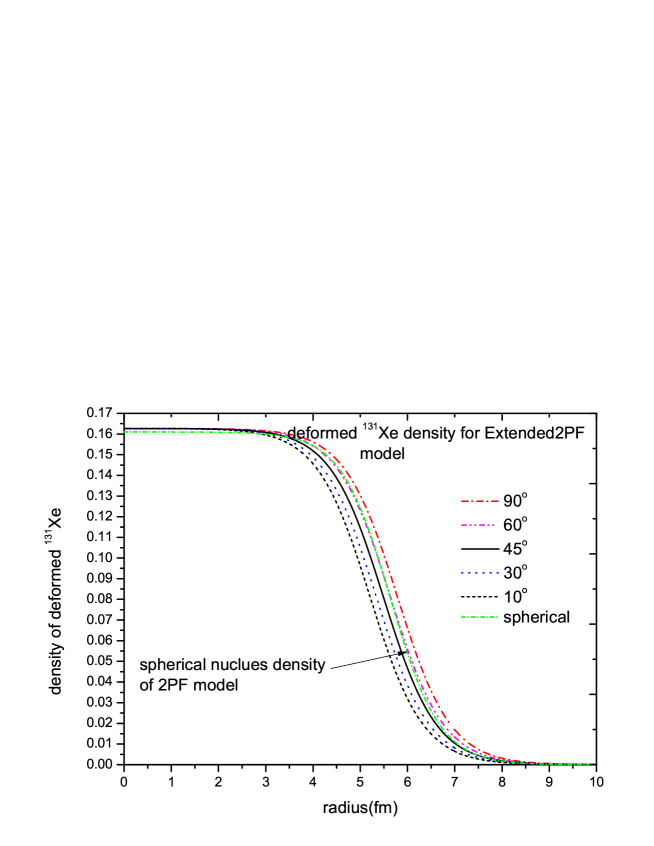
Figure 1: Nuclear density of ¹³¹Xe for the Extended 2PF model. It shows the change of density with increasing angle from 10^∘ to 90^∘, the Short Dash Dot line(green) corresponds to the case of the spherical 2PF model

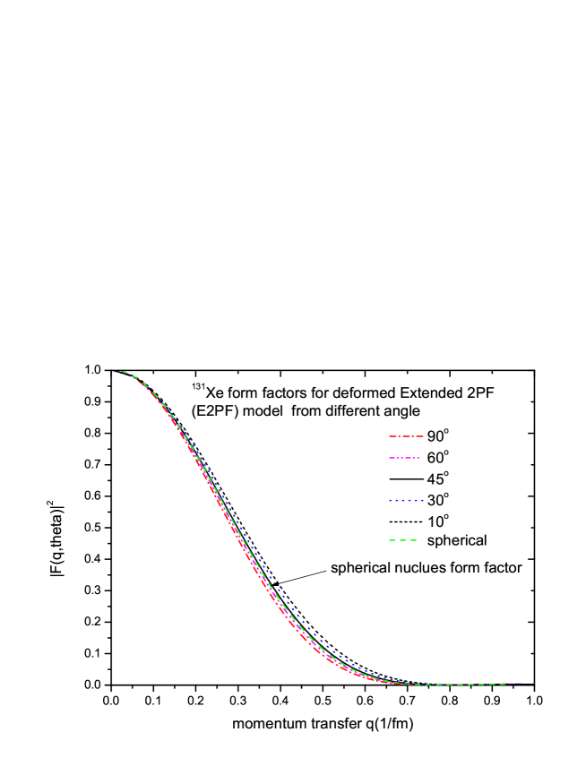
Figure 2: ¹³¹Xe form factors for deformed nucleus Extended 2PF(E2PF)model from different directions: 10^o, 30^o, 45^o, 60^o, 90^o

In Fig.(1) we show the density distribution for ¹³¹Xe in the E2PF model. It is observed that from the center of the nucleus to about three fermis, the density remains unchanged in all directions. Then the angular distribution of the density begins to be apart for different angles beyond three fermis. The short dash dot(green) line is the 2PF density model when the nucleus is assumed to be spherical. Fig.(2) is the corresponding form factors, which are calculated by taking a Fourier transformation to the deformed nuclear density in the configuration space.

II.2 Extension of the Folding model(EF)

There is another commonly adopted model which is rather simple, i.e. the nucleons are postulated to be uniformly distributed in a sphere with a certain boundary radius. For an axially symmetric ellipsoidal shape, one should extend the density for a spherical form. The surface equation of an ellipsoid is

$$\frac{x^{2}}{a^{2}}+\frac{y^{2}}{a^{2}}+\frac{z^{2}}{b^{2}}=1,$$ (7)

or in the spherical coordinate system, it is written as

$$R(\theta)=\sqrt{\frac{a^{2}b^{2}}{(a^{2}-b^{2})\cos^{2}\theta+b^{2}}}.$$ (8)

In an approximation, if we only keep the multiple terms to quadrupole, we can re-parametrize the surface equation to a more convenient one

$$R(\theta)=R_{0}(1+\beta_{2}Y_{20}).$$ (9)

Extending the Folding model, we set the nuclear density to be uniform inside the ellipsoid with radius $R(\theta)$

$$\rho_{0}(r,\theta)=\frac{3M}{4\pi a^{2}b}\Theta(r-R(\theta)),$$ (10)

where $\Theta$ is the step function. Following the literature Helm , we introduce a smearing function $\rho_{1}$ to take care of the soft edge effect of the nucleus:

$$\rho_{1}(r)=\frac{1}{(2\pi s^{2})^{3/2}}\exp(\frac{-r^{2}}{2s^{2}}),$$ (11)

then one should convolve $\rho_{0}$ and $\rho_{1}$ to get the nuclear density

$$\rho(r,\theta) = \int\rho_{0}(\vec{r^{\prime}})\rho_{1}(\vec{r}-\vec{r^{\prime}})d^{3}r^{\prime}$$ (12)

$$= \int\rho_{0}(\vec{r^{\prime}})\rho_{1}(\vec{r}-\vec{r^{\prime}})r^{\prime 2}dr^{\prime}\sin{\theta^{\prime}}d\theta^{\prime}d\varphi^{\prime}$$

$$= \frac{1}{(2\pi s^{2})^{3/2}}\int_{0}^{2\pi}d\varphi^{\prime}\int_{0}^{\pi}\sin{\theta^{\prime}}d\theta^{\prime}\int_{0}^{\infty}\frac{3M}{4\pi a^{2}b}\Theta(r^{\prime}-R(\theta^{\prime}))\times$$

$$\exp(\frac{-(r^{2}+r^{\prime 2}-2rr^{\prime}(\sin\theta\sin\theta^{\prime}\cos(\varphi-\varphi^{\prime})+\cos\theta^{\prime}\cos\theta))}{2s^{2}})r^{\prime 2}dr^{\prime}.$$

The semi-axes $a$ and $b$ are set as

$$a = R(\theta=\frac{\pi}{2})=R_{0}(1+\beta_{2}Y_{20}(\frac{\pi}{2}))=R_{0}(1-\sqrt{\frac{5}{16\pi}}\beta_{2})$$

$$b = R(\theta=0)=R_{0}(1+\beta_{2}Y_{20}(0))=R_{0}(1+2\sqrt{\frac{5}{16\pi}}\beta_{2}).$$ (13)

In the extended Folding (EF) model, we can also calculate the mean square root radius $\bar{R}^{EF}$. For a spherical nucleus, one may equate the mean square root radius obtained in the 2PF and Fold models, thus he acquires the spherical radius $R_{0}$ for the Fold model Duda:2006uk ; JDL .

$$R_{0}=\sqrt{c^{2}+\frac{7}{3}\pi^{2}a^{2}-5s^{2}},\quad c\simeq(1.23A^{1/3}-0.6)\mbox{fm},\quad s=0.9\mbox{fm},a=0.52\mbox{fm}.$$ (14)

As aforementioned, the deformation makes the shape of the nucleus slightly deviate from a spherical form, we can still use the above relation achieved for spherical nuclei and set $R_{0}$ to be the parameter in Eq.(9).

A Fourier transformation would bring the nuclear density to the expected form factor $F(q,\theta)$. It is noted that now the form factor is also direction-dependent.

$$F(q) = \int\rho_{0}({\bf r}^{\prime})\rho_{1}({\bf r}-{\bf r}^{\prime})d^{3}r^{\prime}e^{i{\bf q}\cdot{\bf r}}d^{3}r$$ (15)

$$= \int\rho_{0}({\bf r}^{\prime})d^{3}r^{\prime}\int\rho_{1}({\bf r}-{\bf r}^{\prime})d^{3}r^{\prime}e^{i{\bf q}\cdot{\bf r}}d^{3}r$$

$$= \int_{0}^{\infty}\rho_{0}({\bf r}^{\prime})d^{3}r^{\prime}\int_{0}^{\infty}\rho_{1}({\bf u})e^{i{\bf q}\cdot{\bf r}}d^{3}u\ \quad(\mbox{setting}\quad{\bf r}-{\bf r}^{\prime}={\bf u})$$

$$= \int_{0}^{\infty}\rho_{0}({\bf r}^{\prime})d^{3}r^{\prime}\int_{0}^{\infty}\rho_{1}({\bf u})e^{i{\bf q}\cdot({\bf u}+{\bf r}^{\prime})}d^{3}u$$

$$= \int_{0}^{\infty}\rho_{0}({\bf r}^{\prime})e^{i{\bf q}\cdot{\bf r}^{\prime}}d^{3}r^{\prime}\int_{0}^{\infty}\rho_{1}({\bf u})e^{i{\bf q}\cdot{\bf u}}d^{3}u$$

$$= F_{0}(q)F_{1}(q),$$

and

$$F_{1}(q) = \int\rho_{1}(r)e^{i{\bf q}\cdot{\bf r}}d^{3}r$$ (16)

$$= e^{-{\bf q}^{2}/2}.$$

We take a trick to make the integration easier as ${\bf r}$ is described in the cylindrical coordinate while ${\bf q}$ is described in the spherical coordinate as:

$$\left\{\begin{array}[]{l}x=t\cos\varphi_{1}\\ y=t\sin\varphi_{1}\\ z=z\end{array}\right\}\quad\left\{\begin{array}[]{l}q_{x}=q\sin\theta_{2}\cos\varphi_{2}\\ q_{y}=q\sin\theta_{2}\sin\varphi_{2}\\ q_{z}=q\cos\theta_{2}\end{array}\right\},$$

then

$${\bf q}\cdot{\bf r}=t\cos\phi_{1}q\sin\theta_{2}\cos\phi_{2}+t\sin\phi_{1}q\sin\theta_{2}\sin\phi_{2}+zq\cos\theta_{2},$$

where $t=\sqrt{x^{2}+y^{2}}=\sqrt{r^{2}-z^{2}}$.

Thus we obtain

$$F_{0}(q,\theta_{2}) = \int\rho_{0}(r,\theta)e^{i{\bf q}\cdot{\bf r}}d^{3}r$$ (17)

$$= \int\frac{3M}{4\pi a^{2}b}e^{i(xq_{x}+yq_{y}+zq_{z})}tdtd\varphi_{1}dz$$

$$= \frac{3M}{4\pi a^{2}b}\int e^{i(q\sin\theta_{2}\cos\varphi_{2}t\cos\varphi_{1}+q\sin\theta_{2}\sin\varphi_{2}t\sin\varphi_{1}+q\cos\theta_{2}z)}tdtd\varphi_{1}dz$$

$$= \frac{3M}{4\pi a^{2}b}\int_{0}^{a}e^{iq(t\sin\theta_{2}\cos(\varphi_{2}-\varphi_{1})+z\cos\theta_{2})}tdt\int_{-\sqrt{(1-\frac{t^{2}}{a^{2}})b^{2}}}^{\sqrt{(1-\frac{t^{2}}{a^{2}})b^{2}}}dz\int_{0}^{2\pi}d\varphi_{1}.$$

The parameters $a$ and $b$ are the semi-axes defined above. Thus the form factor in the EF model can be written as:

$$F(q,\theta_{2})=F_{0}(q,\theta_{2})F_{1}(q).$$ (18)

In Figure 3, the ¹³¹Xe density distribution determined by the EF model is shown, while the corresponding form factors are given in Fig.4. The short dash dot(green) line corresponds to the spherical form of the nucleus. For the spherical nucleus, it has already been known that the form factor obtained with the 2PF model is very close to that determined by the Folding modelChen:2011xp . Thus we will also make a comparison between the E2PF and EF form factors at the end of the paper. Then we will present the third model to do the same job in the following section.

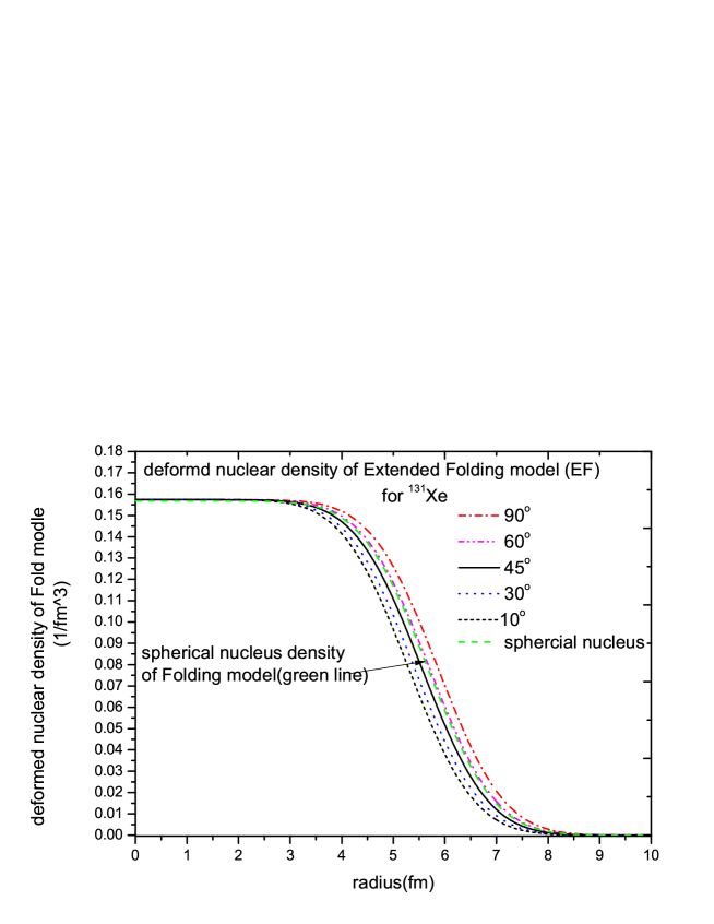
Figure 3: ¹³¹Xe form factors for deformed nucleus of Extended 2PF(E2PF)model from different directions: 10^o, 30^o, 45^o, 60^o, 90^o

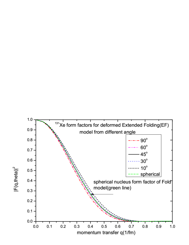
Figure 4: ¹³¹Xe form factors for deformed nucleus determined in the EF model for different directions: 10^o, 30^o, 45^o, 60^o, 90^o

II.3 The Nilsson Mean Field(NMF)

Above, we use two simplified models (E2PF and EF) to derive the form factors for deformed nuclei. The advantage is that the models are simple and we can obtain analytical solution which is convenient for illustrating the characteristics of the form factors, but might be too simplified. Now we turn to use a more realistic model.

In this subsection, the form factors for deformed nuclei are obtained in the Nilsson modified oscillator model, then using ¹³¹Xe as an example, we present the results in some figures.

Below, let us briefly review the model and show how we apply it to study the concerned form factor.

In the Hamiltonian of the Nilsson model the potential for an axially symmetric harmonic oscillator can be written as Nilsson1969 ; Nilsson1958 ; Nilsson1955

$$H={-\hbar^{2}\over 2M}\nabla^{2}+\frac{1}{2}M[\omega_{x}^{2}(x^{2}+y^{2})+\omega_{z}^{2}z^{2}]-C{\bf s}\cdot{\bf l}-D{\bf l}^{2},$$ (19)

where $C{\bf s}\cdot{\bf l}$ is the spin-orbit coupling, and $D{\bf l}^{2}$ flattens the bottom of the potential.

A deformation parameter $\delta$ is introduced to reflect the axial symmetry for the deformed nuclei as

$$\omega_{x}^{2} = \omega_{y}^{2}=\omega_{0}^{2}(\delta)(1+\frac{2}{3}\delta),$$ (20)

$$\omega_{z}^{2} = w_{0}^{2}(\delta)(1-\frac{4}{3}\delta).$$ (21)

The equipotential surface encloses a constant volume if

$$\omega_{x}\omega_{y}\omega_{z}=const.$$ (22)

Then we have

$$\omega_{0}[1-\frac{4}{3}\epsilon_{2}^{2}-\frac{16}{27}\epsilon_{2}^{3}]^{1/6}=\omega_{00}.$$ (23)

The Hamiltonian can be decomposed into three pieces as

$$H = H_{sp}+H_{\epsilon_{2}}-C{\bf s}\cdot{\bf l}-D{\bf l}^{2},$$ (24)

$$H_{sp} = \frac{p^{2}}{2m}+\frac{1}{2}m\omega_{0}^{2}r^{2},$$ (25)

$$H_{\epsilon_{2}} = -m\omega_{0}^{2}r^{2}\frac{2}{3}\epsilon_{2}P_{2}(cos\theta).$$ (26)

It would be convenient to use dimensionless coordinates and parameters which are defined as

$$\rho = \sqrt{\frac{m\omega_{0}r}{\hbar}}r,$$ (27)

$$C = 2\kappa\hbar\omega_{00},$$ (28)

$$D = \frac{1}{2}C\mu=\kappa\hbar\omega_{00}\mu.$$ (29)

Then the Nilsson Hamiltonian can be further written as

$$H = \hbar\omega_{0}(H_{0}-\frac{2}{3}\epsilon_{2}P_{2})-\kappa\hbar\omega_{00}[2{\bf s}\cdot{\bf l}+\mu({\bf l}^{2}-<{\bf l}^{2}>_{N})],$$ (30)

$$H_{0} = \frac{1}{2}(-\nabla_{\rho}^{2}+\rho^{2}),$$ (31)

where $<{\bf l}^{2}>=N(N+3)/2$ is an average over all states within the $N-$th shell, and $\hbar\omega_{00}\approx 41A^{-1/3}$ MeV.

If the octupole and hexadecupole deformations are considered, the Hamiltonian would become more complicated as

$$H=\hbar\omega_{0}(H_{0}+\rho^{2}(-2/3\epsilon_{2}P_{2}+\epsilon_{3}P_{3}+\epsilon_{4}P4))-\kappa\hbar\omega_{00}[2{\bf l}\cdot{\bf s}+\mu({\bf l}^{2}-<{\bf l}^{2}>_{N})]$$ (32)

and it is the Hamiltonian we are going to use in the later part of this paper.

The Nilsson wavefunction is constructed with the spherical harmonic oscillator basis $|Nlj\Omega>$,

$$\Psi_{i}=\sum_{\begin{subarray}{c}\alpha\end{subarray}}\omega_{\alpha}c_{{\alpha}}^{{\dagger}}|0>,$$ (33)

where $\omega_{\alpha}$ is a coefficient, $\alpha$ refers to a set of quantum numbers $(njl\Omega)$ of the harmonic-oscillators.

The nuclear density thus is expressed as

$$\rho=\sum_{\begin{subarray}{c}i=1\end{subarray}}(\Psi_{i}^{\dagger}(\pi)\Psi_{i}(\pi)+\Psi_{\bar{i}}^{\dagger}(\pi)\Psi_{\bar{i}}(\pi))+\sum_{\begin{subarray}{c}i=1\end{subarray}}(\Psi_{i}^{\dagger}(\nu)\Psi_{i}(\nu)+\Psi_{\bar{i}}^{\dagger}(\nu)\Psi_{\bar{i}}(\nu)),$$ (34)

where $\bar{i}$ represents the time-reversed states.

In this paper, the major shells under consideration are from 0 to 9 for proton and neutron, respectively. The quadrupole, octupole and hexadecapole deformation parameters are determined by experimentsnndc , which are -0.108, 0 and 0.027, respectively.

Performing a Fourier transformation on the nuclear density, we obtain the concerned form factor. On the right panel of Fig.(5), the angular dependence of the nuclear density of ¹³¹Xe is shown. Fig.(5) plots the NMF form factors F$(q,\theta)$ with various angles. The left panel of Fig.(6) compares the form factors at direction of $\theta=\pi/6$ obtained with the three models: the EF, E2PF, and NMF, whereas the right panel is the corresponding densities. Fig.(7) shows difference of the form factors F$(q,\pi/6)$ for ⁷³Ge and ¹³¹Xe, as well as their density distributions.

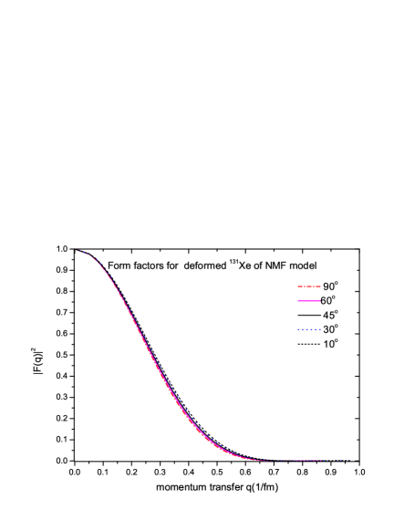
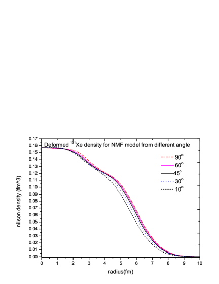
Figure 5: The right panel shows the dependence of the ¹³¹Xe density on the directions from 10^o to 90^o obtained in the Nilsson Mean Field model, the left panel is the form factor

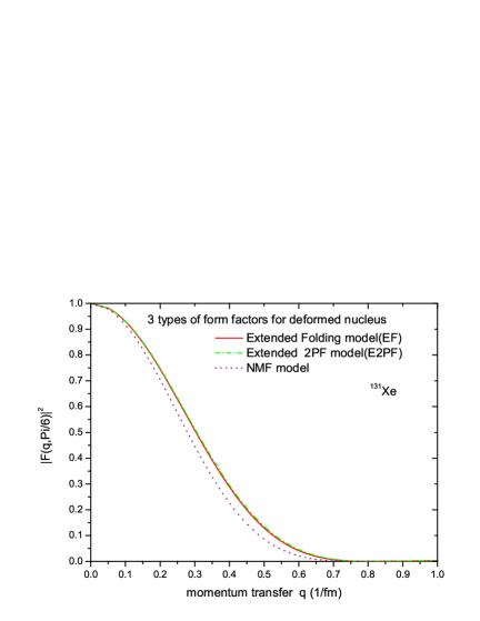
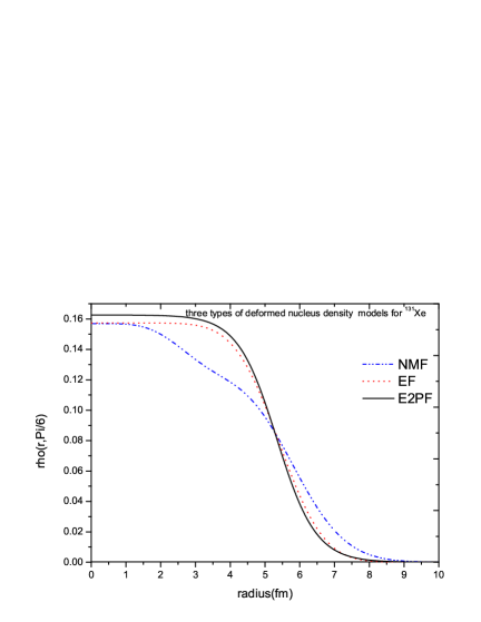
Figure 6: The form factors F(q,$\pi/6$) and density $\rho(r,\pi/6)$ obtained in three different models: E2PF,EF,NMF for ¹³¹Xe

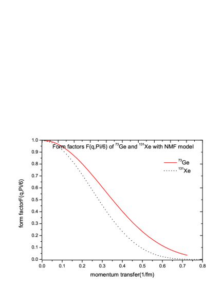
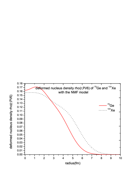
Figure 7: the left graph is the form factors F(q,$\pi/6$) for the ⁷³Ge and ¹³¹Xe with NMF model, the right graph is the density distributions $\rho(r,\pi/6)$.

III Summary

The aim of this work is to study if a small deformation of nuclei can induce observable effects on the form factors for the direct detection of dark matter flux. The form factor, no matter the nuclei are of spherical or deformed shapes, say ellipsoidal, must satisfy two normalization conditions. First, the nuclear density must be normalized as

$$\int\rho(r,\theta,\phi)d^{3}r=M,$$ (35)

where $M$ is the total mass of the nucleus. It is independent of the shape of the nucleus. Secondly, the form factor must satisfy the condition

$$F(|{\bf q}|=0)=F(0)=1.$$ (36)

This condition does not depend on polar and azimuthal angles. With these two conditions, one can adopt different models for the nuclear density and then carry out a Fourier transformation to convert the nuclear density from the configuration space into the momentum space to gain the form factor which corresponds to non-zero momentum transfer.

In this work, we start with the spherical nuclei and adopt three models which are commonly employed to study the nuclear effects. Then we extend them to deformed shapes by including polar angle dependence in the density while an axial symmetry is assumed for simplicity. With the three models we obtain the form factor for the nuclei whose shape slightly deviates from spherical form, namely their ellipticity is relatively small.

We notice from the figures shown in the text that the form factors are not very much apart from that for spherical form, indeed the dependence of the form factor on $|{\bf q}|$ for $\theta=\pi/4$ is rather close to that for spherical shape.

Especially, if there is not a strong magnetic field to polarize the nuclei at very low temperature, the nuclei in the detection material would be randomly oriented, the polar and azimuthal angles would be averaged and the deformation effects should be eventually smeared out.

Therefore, our conclusion is that unless one can keep the detector at very low temperature such as the CDMS detector and apply a strong magnetic field to it, the effects of deformation of nuclei can be safely ignored.

References

- (1) X. G. He, S. Y. Ho, J. Tandean and H. C. Tsai, Int. J. Mod. Phys. D 20, 1423 (2011).
- (2) F. Briscese, AIP Conf. Proc. 1396, 176 (2011).
- (3) K. Cheung, K. Mawatari, E. Senaha, P. Y. Tseng and T. C. Yuan, Int. J. Mod. Phys. D 20, 1413 (2011).
- (4) H. An, S. -L. Chen, R. N. Mohapatra, S. Nussinov, Y. Zhang, Phys. Rev. D82, 023533 (2010). [arXiv:1004.3296 [hep-ph]].
- (5) N. Fornengo, S. Scopel, A. Bottino Phys. Rev.D 83:015001(2011)
- (6) A. Morselli, Prog. Part. Nucl. Phys. 66, 208-215 (2011).
- (7) S. Profumo, AIP Conf. Proc. 1182, 256-258 (2009)
- (8) L. Sonnenschein, [arXiv:1106.4901 [hep-ex]].
- (9) G. Jungman, M. Kamionkowski, K. Griest. Phys. Rept. 267,195 (1996)[arXiv:hep-ph/9506380].
- (10) M.W.Goodmand and E.Witten, Phys. Rew. D 31 (1986) 3059
- (11) M. T. Ressell, M. B. Aufderheide, S. D. Bloom, K. Griest, G. J. Mathews and D. A. Resler, Phys. Rev. D 48, 5519 (1993).
- (12) M. T. Ressell, D. J. Dean, Phys. Rev. C56, 535-546 (1997). [hep-ph/9702290].
- (13) J. Engel, P. Vogel, Phys. Rev. D40, 3132-3135 (1989).
- (14) J. Engel, Phys. Lett. B264, 114-119 (1991).
- (15) M. Drees and C. L. Shan, PoS IDM2008, 110 (2008) [arXiv:0809.2441 [hep-ph]].
- (16) G. Duda, A. Kemper and P. Gondolo, JCAP 0704, 012 (2007).
- (17) Y. -Z. Chen, Y. -A. Luo, L. Li, H. Shen, X. -Q. Li, Commun. Theor. Phys. 55, 1059-1064 (2011). [arXiv:1101.3049 [hep-ph].
- (18) M. J. Brown, W.Greiner. Z. Phys. A 310, 287(1983)
- (19) M. Ismail and EL Gealy, Phys. Lett. B 563, 53 (2003)
- (20) T.Cooper, W.Bertozzi, et, Phys. Rev. C 13 (1976)
- (21) C.Xu, Z.Z.Ren, Phys. Rev. C 73, 041301(2006)
- (22) J.D.Walecka, Theoretical Nuclear Physics and Subnuclear Physics(Oxford University Press,Oxford,1995),pp,11-13
- (23) B.Hahn, D.G.Ravenhall, and R.Hofstadter, Phys. Rev. 101, 1131 (1956)
- (24) A.Bohr and B.R.Mottelson, Nuclear Structure (World Scientific,Singapore,1998),Vol.1.
- (25) M. Ismail, W. M. Seif, A. Y. Ellithi, F. Salah, J. Phys. G G35, 075101 (2008).
- (26) P.Moller, et al, Atom data and nuclear data, 59, 185-381 (1995).
- (27) R. Helm , Phys. Rev.104 1466 (1956).
- (28) J. D. Lewin and P. F. Smith, Astropart. Phys. 6, 87 (1996).
- (29) S.G.Nilsson, et at., Nucl. Phys. A131, 1 1969
- (30) B. R. Mottelson and S. G. Nilsson. Phys. Rev. 99. 1615 (1958)
- (31) S. G. Nilsson. Energy eigenstates of the deformed shell model, Mat. Fys. Medd. Dad. Vid. Selsk. 59:185-381(1955)
- (32) http://t2.lanl.gov/data/astro/molnix96/massd.html