Test for anisotropy in the mean of the CMB temperature fluctuation in spherical harmonic space

Abstract

The standard models of inflation predict statistically homogeneous and isotropic primordial fluctuations, which should be tested by observations. In this paper we illustrate a method to test the statistical isotropy of the mean of the cosmic microwave background temperature fluctuations in the spherical harmonic space and apply the method to the Wilkinson Microwave Anisotropy Probe seven-year observation data. A classical method to test a mean, like the simple Student’s t test, is not appropriate for this purpose because the Wilkinson Microwave Anisotropy Probe data contain anisotropic instrumental noise and suffer from the effect of the mask for the foreground emissions which breaks the statistical independence. Here we perform a band-power analysis with Monte Carlo simulations in which we take into account the anisotropic noise and the mask. We find evidence of a non-zero mean at 99.93 % confidence level in a particular range of multipoles. The evidence against the zero-mean assumption as a whole is still significant at the 99 % confidence level even if the fact is taken into account that we have tested multiple ranges.

I introduction

Inflation provides a successful mechanism of generating primordial density perturbations that give rise to the large-scale structure of the Universe and temperature anisotropy in the cosmic microwave background (CMB). One of the important consequences of inflation models, which should be tested with observations, is that they predict statistically homogeneous and isotropic Gaussian fluctuations with nearly scale invariant power spectrum 2005ppci.conf..235L .

So far, tests of the scale invariance and/or the Gaussianity of primordial fluctuations have been done intensively. In those tests, the statistical homogeneity and isotropy are often implicitly assumed. This assumption, however, should be verified with observational test. For example, the statistical homogeneity of the large-scale structure was tested by comparing the means of the galaxy distributions in different directions 2011CQGra..28p4003S . For the CMB temperature field, the anisotropy of the power spectrum has rigorously been tested, particularly in the context of the hemispherical asymmetry 2004MNRAS.349..313P ; 2004ApJ…605…14E ; 2004ApJ…609.1198E ; 2004MNRAS.354..641H ; 2008PhRvD..78f3531B ; 2009ApJ…704.1448H ; 2009ApJ…699..985H . Similar tests in real space of the mean, variance, skewness and kurtosis were performed in 2008JCAP…08..017L .

In this paper we illustrate a method to test the statistical isotropy of the mean of the CMB temperature fluctuations in the spherical harmonic space, and we apply it to the Wilkinson Microwave Anisotropic Probe (WMAP) seven-year observation data. This method can be potentially useful for the forthcoming PLANCK and future CMB surveys, for which contaminations of the CMB maps by instrumental noises will take place for higher multipole range.

The CMB temperature field can be expressed as a background value $T_{0}$ with associated fluctuations $\Delta T$,

$$T(\hat{n})=T_{0}(\hat{n})+\Delta T(\hat{n})~{},$$ (1)

where $\hat{n}$ is a unit direction vector. Under a null hypothesis that the background $T_{0}$ is isotropic, $T_{0}(\hat{n})=T_{0}$ and the fluctuations $\Delta T(\hat{n})$ defined over the full sky can be expanded in terms of spherical harmonics as

$$\Delta T(\hat{n})=\sum^{\infty}_{\ell=1}\sum^{\ell}_{m=-\ell}a_{\ell m}Y_{\ell m}(\hat{n})~{},$$ (2)

with

$$a_{\ell m}=\int d\Omega(\hat{n})\Delta T(\hat{n})Y^{\ast}_{\ell m}(\hat{n})~{},$$ (3)

where $Y_{\ell m}(\hat{n})$ are the spherical harmonic functions evaluated in the direction $\hat{n}$. If the primordial fluctuations are statistically homogeneous and isotropic in the mean and if they obey the Gaussian distribution, $2\ell+1$ spherical harmonic coefficients $a_{\ell m}$s for each $\ell$ are independent Gaussian variables with the following properties

$$\left<a_{\ell m}\right>=0~{},$$ (4)

and

$$\left<a_{\ell m}a_{\ell^{\prime}m^{\prime}}^{\ast}\right>=\delta_{\ell\ell^{\prime}}\delta_{mm^{\prime}}C_{\ell}~{},$$ (5)

where $\left<\cdot\cdot\cdot\right>$ denotes the ensemble average, $C_{\ell}$ is the ensemble average power spectrum and $\delta$ is the Kronecker symbol.

This null hypothesis that the means of $a_{\ell m}$s are zero [Eq. (4)] should be verified with observation. Our aim of this paper is to test this null hypothesis against the alternative hypothesis that the means of $a_{\ell m}$s are non-zero. One of the difficulties in this test is to decorrelate the neighboring modes in harmonic space whose correlations are caused by a cut sky mask. In order to overcome this problem, we use the band-power decorrelation analysis following the method in 2008PhRvD..78l3002N . The method is to decompose the correlated spectrum to mutually independent band-power spectrum by diagonalizing the covariance matrix. We run Monte Carlo simulations to calculate the covariance matrix of the mean distribution, including anisotropic instrumental noise and the effect of the mask.

Recently, Armendariz-Picon tested this zero-mean hypothesis in a smart analytic way with a symmetric cut sky mask to obtain uncorrelated and independent variables, with the noise contributions neglected 2011JCAP…03..048A . The author found significant evidence for nonzero means of $a_{\ell m}$s in a particular multipole range. He concluded, however, that this evidence is statistically insignificant because the signal is high only at one bin among eight different multipole bins. The main difference between our analysis and his is that we make extensive use of Monte Carlo simulations to keep the cosmological information as much as possible while taking into account the noise contributions and the effect of the WMAP mask.

This paper is organized as follows. In Sec. II we briefly review the main properties of the CMB temperature field, its spherical harmonic analysis and the cut sky mask. We describe the method of our analysis based on Monte Carlo simulations with the WMAP seven-year data in Sec. III. Our results are presented in Sec. IV and we provide a discussion in Sec. V. We conclude our findings in Sec. VI.

II Temperature field and Mask

The temperature field $\Delta T_{\mathrm{obs}}$ observed with instruments involves a convolution with the detector beam window $B$ and the detector noise $\Delta T_{\mathrm{noise}}$. In addition, since we have to divide the all sky into finite pixels, we introduce a pixel smoothing kernel $K$, and write the temperature field as

$$\Delta T_{\mathrm{obs}}=K\ast\left[B\ast\Delta T_{\mathrm{real}}+\Delta T_{\mathrm{noise}}\right]~{},$$ (6)

where the star “$\ast$” denotes the convolution and $\Delta T_{\mathrm{real}}$ is a superposition of CMB temperature field $\Delta_{\mathrm{CMB}}$ and foreground emission $F$;

$$\Delta T_{\mathrm{real}}(\hat{n})=\Delta T_{\mathrm{CMB}}(\hat{n})+F(\hat{n}).$$ (7)

The foregrounds consist of, for example, the dust emission and synchrotron radiation from our own Galaxy and emissions from extragalactic objects. The WMAP team provides the sky map data with the foregrounds reduced by using appropriate foreground templates 2011ApJS..192…15G . However, the cleaning procedure does not completely remove the foreground contamination along the galactic disk and that from extragalactic objects. To avoid the effect of the residual foreground, the contaminated regions have to be masked out. The mask is defined by a position-dependent weight function $M(\hat{n})$ as

$$M\left(\hat{n}\right)=\left\{\begin{array}[]{ll}0&\qquad\mbox{for contamination region}\\ 1&\qquad\mbox{otherwise}.\\ \end{array}\right.$$ (10)

By definition, $M\left(\hat{n}\right)\left[K\ast B\ast F\right]\left(\hat{n}\right)=0$. Then, by construction, we get the masked sky $\Delta T_{M}$ which does not include foregrounds,

$$\Delta T_{\mathrm{M}}\left(\hat{n}\right)=M\left(\hat{n}\right)\left[K\ast B\ast\Delta T_{\mathrm{CMB}}+K\ast\Delta T_{\mathrm{noise}}\right]\left(\hat{n}\right).$$ (11)

Equations (4) and (5) state that the $2\ell+1$ variables $a_{\ell m}$ form a set of normally distributed independent variables with a variance $C_{\ell}$. However, in reality, we cannot obtain the true $a_{\ell m}$ but only the pseudo $a_{\ell m}$ ($a^{\mathrm{mask}}_{\ell m}$) from the masked sky map. Rewriting Eq. (11) in harmonic space, a $a^{\mathrm{mask}}_{\ell m}$ from the masked sky map is given by

$$a^{\mathrm{mask}}_{\ell m}=\sum_{\ell^{\prime}m^{\prime}}M_{\ell m,\,\ell^{\prime}m^{\prime}}a^{\mathrm{all\,sky}}_{\ell m}~{},$$ (12)

where $a^{\mathrm{all\,sky}}_{\ell m}$ is from the all sky CMB map which we can never obtain and $M_{\ell m,\,\ell^{\prime}m^{\prime}}$ is the convolution matrix of the mask. The detector pixel noise is well described by a Gaussian distribution with zero mean as shown in the WMAP papers 2003ApJS..148…29J ; 2007ApJS..170..263J . Therefore if ensemble averages of true $a_{\ell m}$s are zero, $\left<a_{\ell m}^{\mathrm{all\,sky}}\right>=0$, the ensemble averages of pseudo $a_{\ell m}$s are zero, $\left<{a^{\mathrm{mask}}_{\ell m}}\right>=0$. The details of the convolution matrix are not essential in the present analysis, but the matter of importance is that $a_{\ell m}$s have correlations with neighboring modes.

III Data and Analysis

III.1 Data

For the main analysis in this paper, we use the WMAP seven-year foreground-reduced sky maps 2011ApJS..192…14J from differential assemblies (DAs) Q1, Q2, V1, V2, and W1, W2, W3, W4, pixelized in the HEALPix 2005ApJ…622..759G sphere pixelization scheme with the resolution parameter $N_{\mathrm{side}}=512$. These sky maps are provided at the LAMBDA web site LAMBDAwebsite . We co-added them using inverse noise pixel weighting and form either individual frequency combined maps (Q, V, W) or an overall combined map (Q+V+W) to increase the signal to noise ratio according to

$$T(i)=\frac{1}{W(i)}\sum^{j_{e}}_{j=j_{s}}w_{j}(i)T_{j}(i)~{},$$ (13)

where $i$ and $j$ are the pixel and DA indices, respectively. The noise weighting function $w_{j}(i)$ is given by $w_{j}(i)=N^{\rm obs}_{j}(i)/\sigma^{2}_{0j}$, where $\sigma_{0j}$ is the noise root-mean square for the $j$th DA, and $N^{\mathrm{obs}}_{j}(i)$ is the number of observations of the $i$th pixel for the $j$th DA, and $W(i)=\sum^{j_{e}}_{j_{s}}w_{j}(i)$.

For the mask, to eliminate foreground contamination, we use the extended temperature analysis mask (KQ75y7 sky mask) 2011ApJS..192…14J .

We use a power spectrum $C_{\ell}$ file and a beam transfer function file to produce realizations of the temperature map. The power spectrum $C_{\ell}$ we use is the best fitting $C_{\ell}$ to the WMAP seven-year data set 2011ApJS..192…16L in the $\Lambda$CDM (+sz+lens) model. The $C_{\ell}$ and the beam transfer function of each DA are also available at the LAMBDA web site.

Our conclusions are based on the results with the overall combined map (Q+V+W). However, we analyze also the individual frequency maps (Q, V, W) to examine effects of the residual foreground emissions and the anisotropic instrumental noise. Because their properties are different for frequency bands.

III.2 Monte Carlo simulation

We carry out Monte Carlo simulations to test whether the temperature map observed by the WMAP has indeed zero mean in harmonic space. Our analysis consists of four steps. First, we prepare 10 000 realizations of the sky map from the normally distributed $a_{\ell m}$s generated from the same underlying power spectrum. Second, we apply the cut sky mask to these Gaussian maps and the temperature maps obtained by the WMAP, and extract $a^{\mathrm{mask}}_{\ell m}$s from each map through the harmonic analysis. Third, for the set of $a^{\mathrm{mask}}_{\ell m}$s obtained in the previous step, we calculated the means of $a^{\mathrm{mask}}_{\ell m}$s for each multipole moment $\ell$. Finally, we decompose the correlated spectrum of the mean to the independent band spectrum and calculate $p$ values of the WMAP observed values by comparing with the distributions realized by simulations.

The method of generating Gaussian sky maps consists of three steps described in detail below. There are two important points in generating Gaussian sky maps. The first is that Gaussian maps should be generated using the same power spectrum as the WMAP sky map. The second is that we must add random noise taking into account the inhomogeneous nature of $N_{\mathrm{obs}}$ to each Gaussian sky map.

Step 1 : Generate the pure Gaussian sky maps

We prepared 10 000 Gaussian sky maps by HEALPix IDL facility isynfast for each DA, which are generated from standard normally distributed random $a_{\ell m}$s from a given power spectrum $C_{\ell}$. The $C_{\ell}$ inputted is the best-fit ($\Lambda$CDM (+sz+lens) model ) of the WMAP seven-year data set. The resolution of the maps is $N_{\mathrm{side}}=512$ which is the same as the resolution of WMAP data we use. We use the same random seed array for all DAs. That is, we generate random sample of 10 000 different universes.

Step 2 : Add noise

According to the WMAP team 2003ApJS..148…29J ; 2007ApJS..170..263J , the instrumental noise is expected to exhibit a Gaussian distribution and the noise variance in a given pixel is inversely proportional to the number of observations of that pixel, $N_{\mathrm{obs}}$. The rms noise per observation $\sigma_{0}$ for each DA is given by the WMAP team. Since a Gaussian map generated by isynfast contains no noise, the noise should be added on it. We add random noise considering the inhomogeneity of $N_{\mathrm{obs}}$ to all pure Gaussian maps.

Step 3 : Combine Gaussian maps

We combine Gaussian maps whose seed number is the same using Eq. (13) and form either individual frequency maps (Q, V, W) or an overall combined map (Q+V+W).

III.3 Test Statistic

Throughout this analysis we deal with real coefficients. The real coefficients $a_{\ell m}$s and conventional complex coefficients $\mathcal{A}_{\ell m}$s are related to each other by

$$a_{\ell m}=\left\{\begin{array}[]{lll}-\sqrt{2}\,\mathrm{Im}\,\mathcal{A}_{\ell-m}&&\mbox{if }m<0\\ \mathcal{A}_{\ell m}&&\mbox{if }m=0\\ \sqrt{2}\,\mathrm{Re}\,\mathcal{A}_{\ell m}&&\mbox{if }m>0.\end{array}\right.$$

We define the mean spectrum as

$$M_{\ell}=\frac{\sum_{m=-\ell}^{\ell}a^{\mathrm{mask}}_{\ell m}/\sqrt{\mathrm{Var}_{\ell}}}{\sqrt{2\ell+1}}~{}.$$ (14)

Here $\mathrm{Var}_{\ell}$ is the average of the variance of $a_{\ell m}$s calculated from the 10 000 realizations,

$$\mathrm{Var}_{\ell}=\frac{1}{\mathcal{N}}\sum_{\alpha=1}^{\mathcal{N}}\frac{\sum_{m}a^{\mathrm{mask},\alpha}_{\ell m}}{2\ell+1}~{},$$ (15)

where $a^{\mathrm{mask},\alpha}_{\ell m}$ represents the multipole coefficient of the $\alpha$th realization and $\mathcal{N}=10000$ is the total number of realizations. This mean spectrum is normalized by the number of samples in a given $\ell$, namely, $2\ell+1$.

The neighboring $\ell$ modes of the mean spectra are strongly correlated with each other, and the number of independent modes is much smaller. To obtain statistically independent variables, we define the binned mean spectrum $\mathcal{M}_{i}$ as,

$$\mathcal{M}_{i}=\frac{\sum_{\ell=\ell_{-,i}}^{\ell_{+,i}}\sum_{m=-\ell}^{\ell}a^{\mathrm{mask}}_{\ell m}/\sqrt{\mathrm{Var}_{\ell}}}{\sqrt{\sum_{\ell=\ell_{-,i}}^{\ell_{+,i}}(2\ell+1)}}~{},$$ (16)

where $i$ is the index of the multipole bin from $\ell=\ell_{-,i}$ to $\ell=\ell_{+,i}$. This binned statistical variable is normalized by the sample number in a bin, i.e., $\sum_{\ell=\ell_{-,i}}^{\ell_{+,i}}(2\ell+1)$.

The covariance matrix of $\mathcal{M}_{i}$ is defined by

$$K_{ij}\equiv\frac{1}{\mathcal{N}}\sum_{\alpha=1}^{\mathcal{N}}\mathcal{M}^{\alpha}_{i}\mathcal{M}^{\alpha}_{j}~{},$$ (17)

where $\mathcal{M}_{i}^{\alpha}$ represents the value of the $i$th multipole bin in the $\alpha$th realization. $K$ is a real symmetric matrix with its dimension equal to the number of multipole bins, $N$, and it can be diagonalized by a real unitary matrix $U$,

$$UKU^{\dagger}=\mbox{diag}(\lambda_{1},\,\lambda_{2},...,\,\lambda_{N})\equiv\Lambda~{},$$ (18)

where $\lambda_{i}$’s the eigenvalues of $K$. A window matrix $W$ is defined as 2008PhRvD..78l3002N

$$W_{ij}=\frac{(K^{-1/2})_{ij}}{\sum^{N}_{m=1}(K^{-1/2})_{im}}~{},$$ (19)

where

$$K^{-1/2}\equiv U^{\dagger}\Lambda^{-1/2}U~{},$$ (20)

and

$$\Lambda^{-1/2}\equiv\mbox{diag}(\lambda_{1}^{-1/2},\,\lambda_{2}^{-1/2},...,\,\lambda_{N}^{-1/2})~{}.$$ (21)

We define a new decorrelated statistical variable $S^{\alpha}_{i}$ by using the window matrix as

$$S_{i}^{\alpha}\equiv\sum^{N}_{j=1}W_{ij}\mathcal{M}^{\alpha}_{j}~{}.$$ (22)

Then the correlation matrix of the variable is diagonal and reads

$$\frac{1}{\mathcal{N}}\sum^{\mathcal{N}}_{\alpha=1}S^{\alpha}_{i}S^{\alpha}_{j} = \left(WK^{t}W\right)_{ij}$$ (23)

$$= \left[\sum_{m=1}^{N}\left(K^{-1/2}\right)_{im}\right]^{-2}\delta_{ij}~{},$$

where ${}^{t}W$ denotes the transposed matrix.

IV Result

We calculate the mean spectrum, $M_{\ell}$, over the multipole range from $\ell=1$ to $\ell=300$ of the WMAP seven-year data, which is shown in Fig. 1.

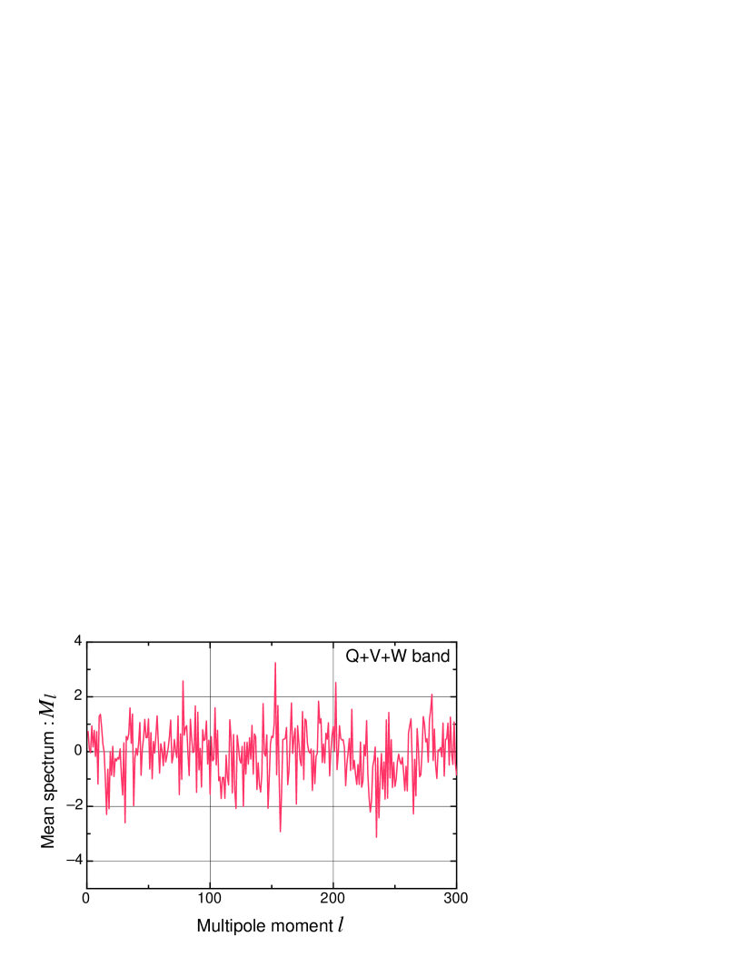
Figure 1: The mean spectrum, $M_{\ell}$, of the overall combined map (Q+V+W), defined in Eq. (14).

Figure 2 shows the covariance matrix of $M_{\ell}$ calculated for 10 000 realizations made by Monte Carlo simulations.

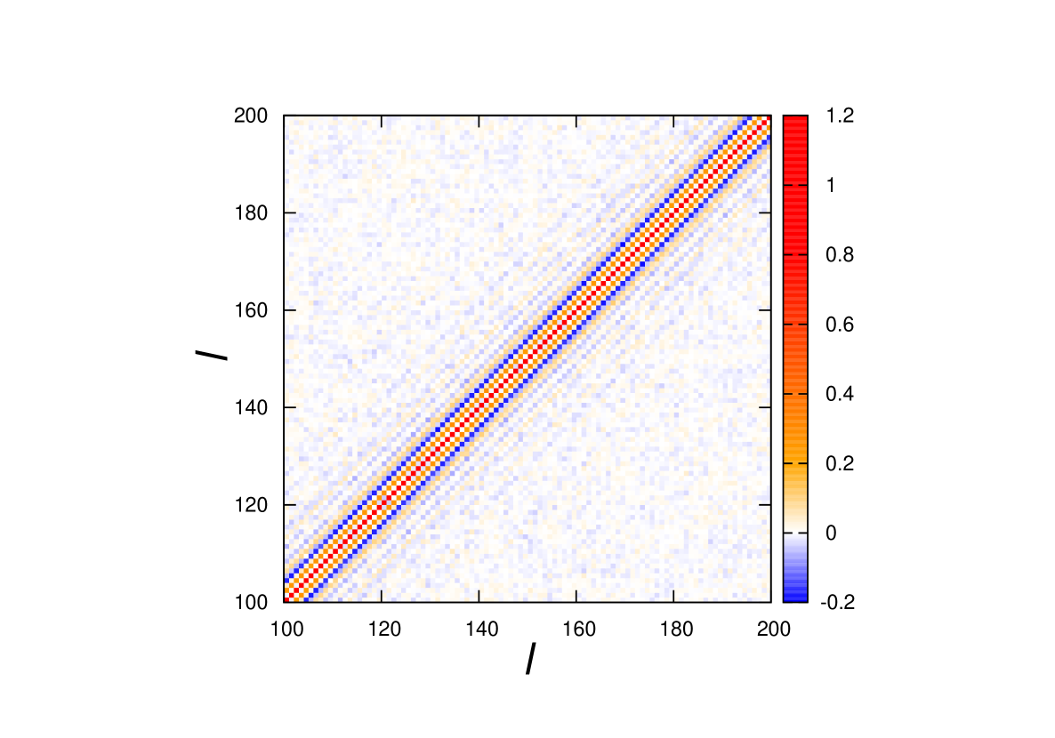
Figure 2: The covariance matrix of the mean spectrum, $M_{\ell}$, calculated by Monte Carlo simulations. The central red strip is diagonal element array and the surrounding blue strips indicate negative correlation. Only a part ($100\leq\ell\leq 200$) of the covariance matrix whose dimension is 300 is shown here.

We can see that neighboring $\ell$ modes are correlated with each other up to the range $\Delta\ell\sim 10$.

Therefore we divide multipole range from $\ell=1$-$300$ into the bins whose size is $\Delta\ell=6$, $10$, or $20$ to calculate the binned mean spectrum, $\mathcal{M}_{i}$. We calculate the covariance matrix $K_{ij}$ defined by Eq. (17) and the window matrix $W_{ij}$ defined by Eq. (19). Then we construct decorrelated statistical variables of the WMAP seven-year data using $W_{ij}$.

The decorrelated band mean spectra of the WMAP seven-year data are represented in Fig. 3. In these panels, the solid line indicates the results from the combined map (Q+V+W),

$$S_{i}=\sum^{N}_{j=1}W_{ij}\mathcal{M}_{j}~{}.$$ (24)

The box represents the standard deviation for each multipole bin,

$$\sigma_{i}=\left[\frac{1}{\mathcal{N}}\sum^{\mathcal{N}}_{\alpha=1}\left(S^{\alpha}_{i}\right)^{2}\right]=\left[\sum_{m=1}^{N}\left(K^{-1/2}\right)_{im}\right]^{-1}~{},$$ (25)

and the bin size are taken as $\Delta\ell=6$, $10$ or $20$ in calculating the binned mean spectrum, $\mathcal{M}_{i}$. The color data points show the results from the individual frequency maps (Q, V, W).

We can see, in the top panel and the middle panel in Fig. 3, that the data points in the multipole range $\ell\sim 210$-$260$ are localized in the negative side as a cluster despite the fact that these data points are random and mutually independent. This negative localization is clearly evident in the lower panel in Fig. 3 where the bin width is taken as $\Delta\ell=20$. It is particularly worth noting that 12th data point (on the multipole bin $\ell=221$-$240$) indicates the nonzero mean evidence with 99.93% confidence level [C.L.] ($\alpha$ ($p$ value) $=$ 0.068%) for the combined map (Q+V+W). Figure 4 and Table 1 show the $p$ values of the data points in the lower panel in Fig. 3. Clearly, the significance is above at the 99% confidence level even for the individual Q, V, W maps, and in fact, for the V, W maps the significance becomes even larger above the 99.9% C.L.

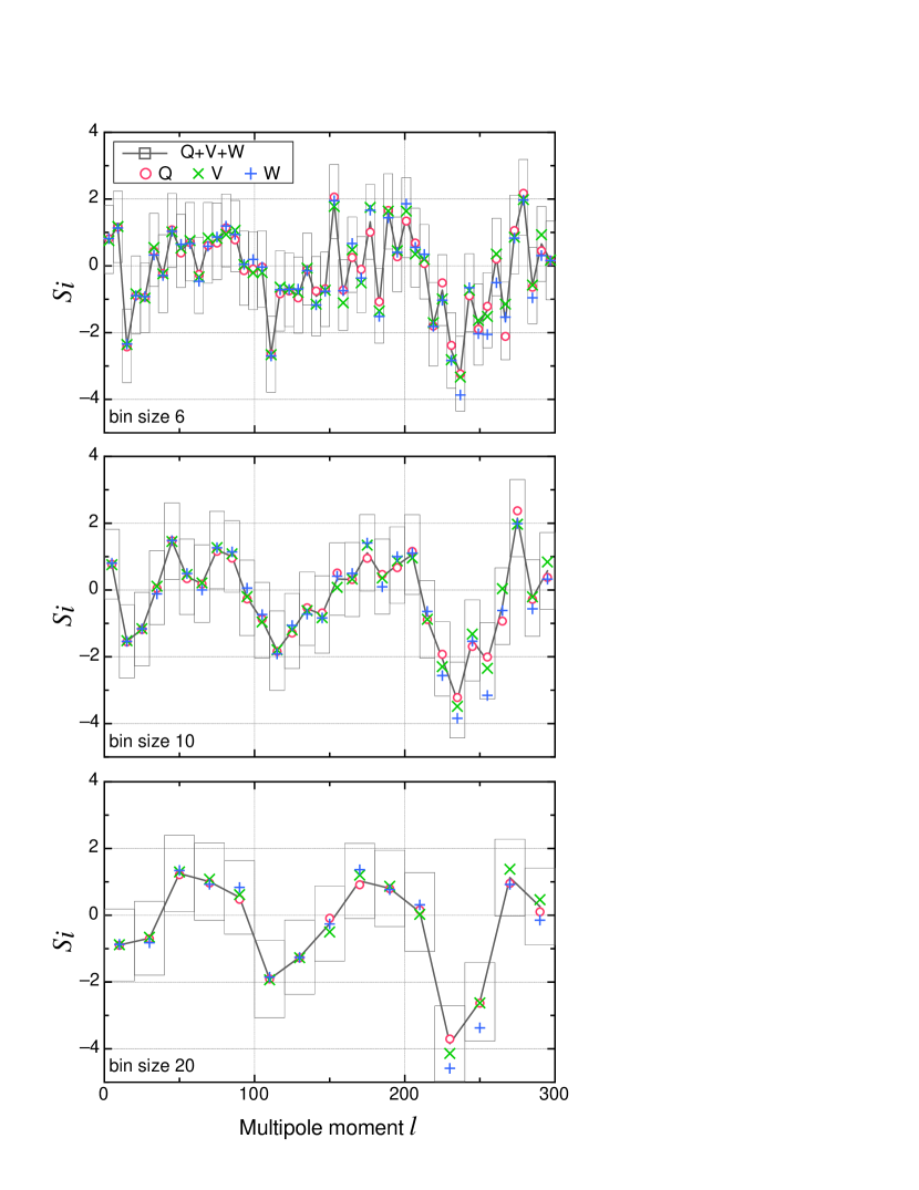
Figure 3: The decorrelated band mean spectrum obtained by the seven-year WMAP data. The boxes and solid line are the result of the overall combined map (Q+V+W) and color data points are the results of the individual frequency maps (Q, V, W). The horizontal width of boxes indicates the bin size $\Delta\ell=6$ (top panel), 10 (middle panel) and 20 (lower panel) for calculating the binned mean spectrum, $\mathcal{M}_{i}$.

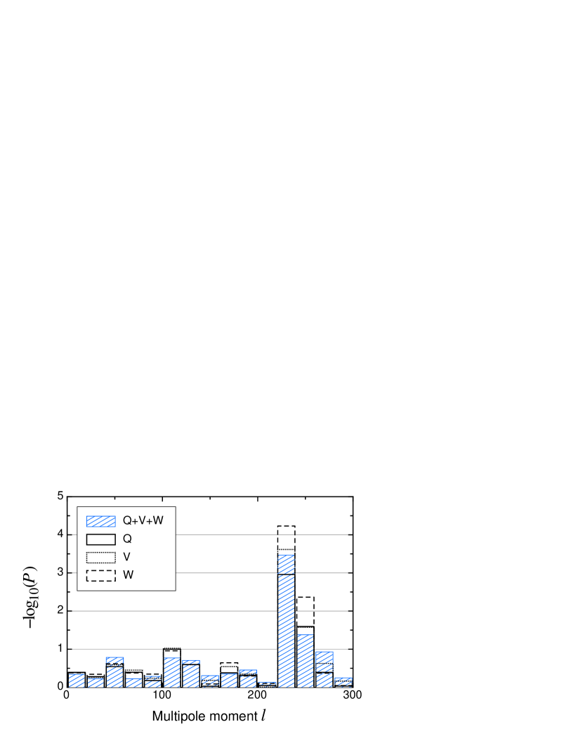
Figure 4: The $p$ values of the data points in the lower panel in Fig. 3, for the bin size $\Delta\ell=20$.

V Discussion

Since in the WMAP observation data the instrumental noise becomes dominant at higher multipoles (see Appendix A), We have used the multipole range up to $\ell=300$. The method we have described can be useful for the forthcoming PLANCKs and future CMB surveys , for which contaminations of the CMB maps by the instrumental noises will take place for higher multipole range.

We can see that the statistics in the above-mentioned figures exhibit the same behavior across the three frequency bands (Q, V, W). Therefore it does not seem that these results are due to residual foregrounds and/or detector noise characteristics which depends on the frequency band, but the cosmological CMB signals.

To eliminate residual foreground emissions more conservatively and confirm these results, we repeat the same analysis with a more extensive mask which cuts the region in galactic latitude $|b|\leq 30^{\circ}$ in addition to KQ75y7 sky mask 2011ApJS..192…14J . Again we obtain consistent results, and in fact, the significance becomes even larger against the zero mean hypothesis as shown in Figs. 5 and 6. The $p$ values are summarized in Table 1. The $p$ value of the 12th multipole bin $\ell=221$-$240$ goes down to $\alpha=0.034\%$ from 0.068%, albeit the standard deviation $\sigma$ becomes larger due to the loss of the sky area to analyze.

Among these analyses of three bin sizes, the results of the bin size $\Delta\ell=6$ keep the original information of the CMB signal as much as possible and represent the finest structure of the means of $a_{\ell m}$s. However, we find that the most intriguing results are for $\Delta\ell=20$ because they represent the negative localization of the means in the multipole range $\ell=221$-$240$ most significantly.

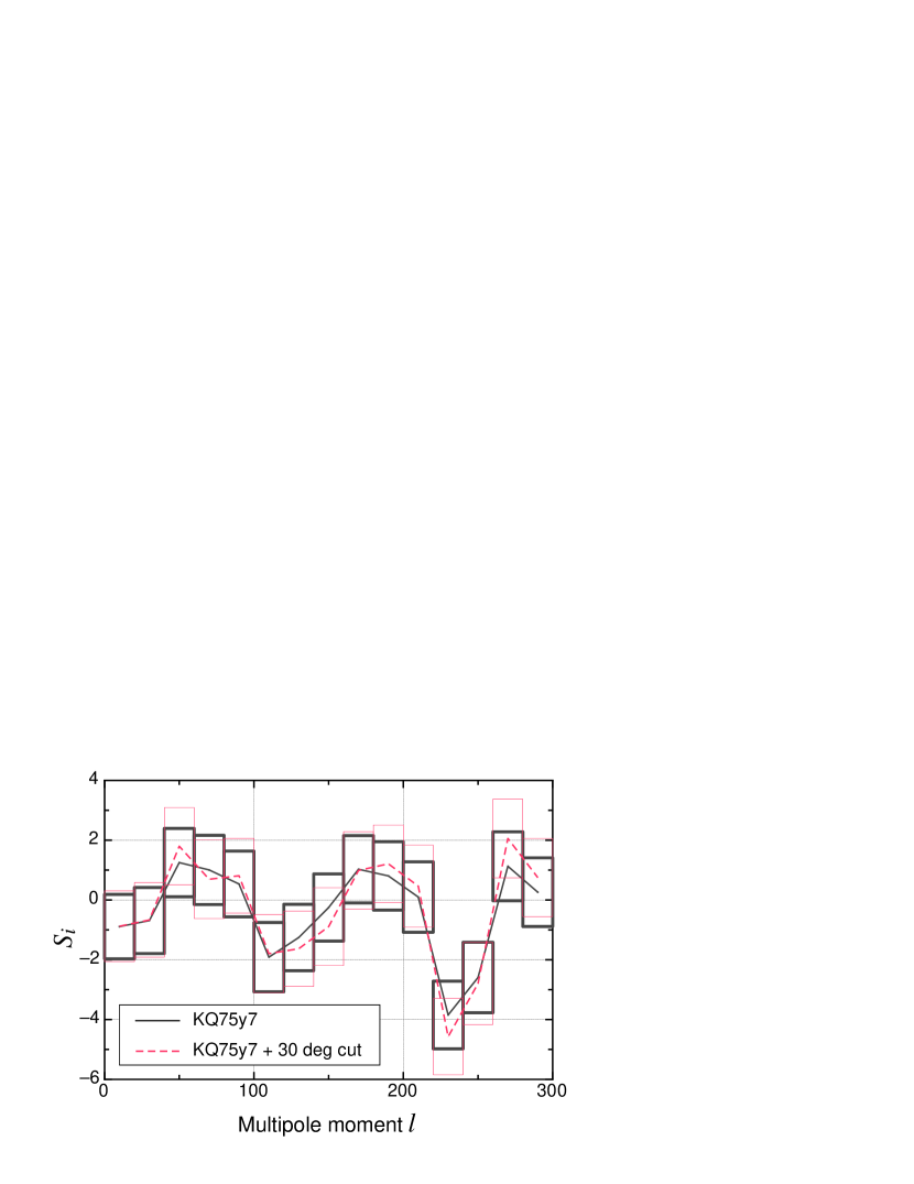
Figure 5: The decorrelated band mean spectra for two different masks. The black solid line (thick boxes) is the result for the conventional mask (KQ75y7) and the red dashed line (thin boxes) is for the more expansive mask (KQ75y7 + cut $|b|\leq 30^{\circ}$).

Figure 6: The $p$ values of data points in Fig. 5.

Table 1: The $p$ values for each CMB map with the KQ75y7 mask (Q, V, W and Q+V+W) and the extensive mask(KQ75y7 + cut $|b|\leq 30^{\circ}$) (Q+V+W only). The bin column indicates the multipole bounds for calculation the binned mean spectrum, $\mathcal{M}_{i}$. The $p$ value is anomalously small in 12th multipole bin $\ell=221$-$240$.

bin			KQ75y7 mask					+ $30^{\circ}$ cut
$\ell_{\mathrm{min}}$	$\ell_{\mathrm{max}}$		Q	V	W	Q+V+W		Q+V+W
1	20		40.5%	41.4%	41.7%	40.9%		45.7%
21	40		52.4%	55.1%	45.5%	53.3%		59.3%
41	60		28.7%	25.6%	24.0%	27.4%		16.4%
61	80		40.3%	35.3%	42.1%	38.5%		59.7%
81	100		66.3%	57.6%	45.0%	62.7%		51.6%
101	120		10.0%	9.44%	11.1%	9.87%		17.0%
121	140		25.3%	25.5%	25.3%	25.9%		19.7%
141	160		93.7%	65.6%	81.6%	82.2%		49.4%
161	180		41.6%	28.6%	22.7%	36.1%		44.7%
181	200		48.4%	45.0%	50.3%	48.1%		35.1%
201	220		89.4%	98.0%	79.2%	93.3%		73.6%
221	240		0.110%	0.024%	0.006%	0.068%		0.034%
241	260		2.53%	2.66%	0.431%	2.78%		4.20%
261	280		40.5%	23.6%	42.5%	32.8%		11.8%
281	300		92.8%	68.8%	90.0%	82.0%		56.6%

On ground that we have tested $n=15$ independent bins, we should evaluate significance as a whole to draw a conclusion against the null hypothesis. If we would like to advocate the anomalousness of the 12th multipole bin in the lower panel in Fig. 3 at the significant level $\alpha_{\mathrm{tot}}$, we should require the $\alpha$ of each individual test to satisfy

$$1-\alpha_{\mathrm{tot}}=(1-\alpha)^{n}~{}.$$ (26)

For $n=15$ independent bins and $\alpha_{\mathrm{tot}}=5\%$, this yields $\alpha=0.34\%$, and for $\alpha_{\mathrm{tot}}=1\%$, $\alpha=0.067\%$. Table 2 represents the values of $\alpha$ of the 12th multipole bin and the corresponding values of $1-\alpha_{\mathrm{tot}}$ for the combined map (Q+V+W) and the individual Q, V, W maps. Clearly, this evidence against the zero-mean hypothesis is still significant, keeping the 99% C.L. (Q+V+W).

Table 2: The values of $\alpha$ of the 12th bin and the corresponding values of $1-\alpha_{\mathrm{tot}}$.

	KQ75y7		KQ75y7 + 30 deg cut
	$\alpha_{\mathrm{12th}}$	$1-\alpha_{\mathrm{tot}}$	$\alpha_{\mathrm{12th}}$	$1-\alpha_{\mathrm{tot}}$
Q+V+W	0.068%	99.0%	0.034%	99.5%
Q	0.110%	98.4%	-	-
V	0.024%	$\geq$ 99.9%	-	-
W	0.006%	$\geq$ 99.9%	-	-

The results we have obtained in this paper would pose a challenge to the statistical isotropy and homogeneity hypothesis in cosmology, and they should be examined through other independent tests. It will be interesting to test in real space for scales corresponding to $220\lesssim\ell\lesssim 240$. For example, a regional test of the power spectrum was performed using a set of circular regions in real space 2004ApJ…605…14E , and similar analyses were done using different size and shape regions in 2008JCAP…08..017L . Räth et al. studied scale-dependent non-Gaussianities in a model-independent way and found significant anomalies in the multipole range $\ell=120$-$300$ 2009PhRvL.102m1301R ; 2011MNRAS.415.2205R ; 2011AdAst2011E..11R . Since we are intrigued with the scales at $220\lesssim\ell\lesssim 240$, we should perform an analysis using finer segmentations.

Can inflationary cosmology explain the anomalous feature found in this paper? Interesting discussions have been done, for example, in 2009PhRvD..80b3526D ; 2008PhRvD..78l3520E ; 2010PhRvD..81h3501C . Although inflation tends to create homogeneous and isotropic fluctuations in the mean and variance, they are on top of the initially inhomogeneous and anisotropic background universe. Hence the fluctuations could be statistically inhomogeneous and anisotropic in total. Another reason would be that our universe is indeed anisotropic: even if CMB fluctuations are statistically homogeneous and isotropic, the CMB photons travel through the inhomogeneous universe, and the gravitational lensing effects could impose statistically anisotropic correlations 2011arXiv1111.3357Rb . In this case, the fluctuations are statistically homogeneous and isotropic in ensemble average, and the anomaly we find is a merely statistical fluctuation due to a particular realization of the universe. It is worth studying how probable the observed inhomogeneous universe can create an apparently anisotropic signal in the mean of the CMB temperature fluctuations in harmonic space through the gravitational lensing effect.

VI Conclusion

We have illustrated the method to test the statistical isotropy of the mean of the full sky CMB temperature fluctuations, which can be potentially useful for the forthcoming PLANCK data and future CMB surveys.

By applying the method to the WMAP seven-year observation data, We have found a significant evidence for a non-zero mean of spherical harmonic coefficients $a_{\ell m}$s at the multipole bin $\ell=221$-$240$, for the combined Q+V+W map at the 99.93% confidence level with the KQ75y7 mask. Using the more extensive mask, the significance becomes larger, at the 99.96% C.L. As a whole, despite the 15 individual tests, this evidence against the zero-mean hypothesis is still significant, keeping above the 99% C.L. This implies that we should challenge the zero-mean assumption and the Universe could contain patterns on the characteristic scales.

However, since there might be unknown systematics, independent observations like PLANCK are awaited for further understanding.

VII Acknowledgments

We would like to thank N. Sugiyama and S. Yokoyama for encouragements, and B. Lew for his kind correspondences and useful discussions at the early stage of this work. Some of the results in this paper have bean obtained using the HEALPix 2005ApJ…622..759G package. We acknowledge the use of the Legacy Archive for Microwave Background Data Analysis (LAMBDA). Support for LAMBDA is provided by the NASA Office of Space Science. This work has been also supported by the Grant-in-Aid for the Scientific Research Fund (20740105, 23340046: TTT, 22012004: KI) commissioned by the Ministry of Education, Culture, Sports, Science and Technology (MEXT) of Japan. We have been partially supported from the Grand-in-Aid for the Global COE Program “Quest for Fundamental Principles in the Universe: from Particles to the Solar System and the Cosmos” from the MEXT.

Appendix A contribution from the instrumental noise

In order to assess the confidence levels of our findings we have performed Monte Carlo simulations in which we took into account the anisotropic noise and the mask. Based on the results of the simulations, we advocated anomalies in the means of multipole coefficients $a_{\ell m}$s. Nevertheless you may think that the anomalies are due to the anisotropic noise. We cannot rebut completely this suspicion because we will never know the exact information of particular realization of the instrumental noise contained in the WMAP data. However, it is possible to estimate the contribution from the anisotropic noise in the mean statistics by performing the same analysis for the CMB-free combination maps (W1-W2, V1-V2, Q1-Q2) , which are mainly determined by the instrumental noise.

Figure 7 shows the results, over plotted on the lower panel in Fig. 3.

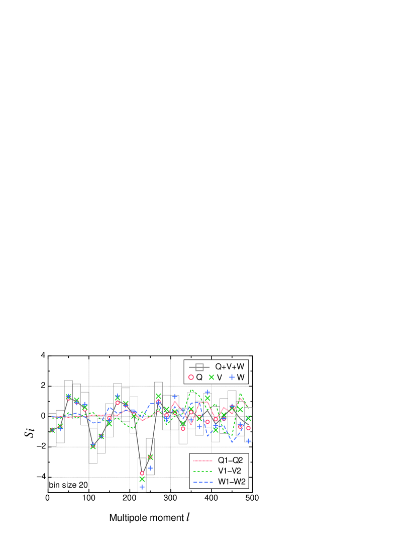
Figure 7: The result from the CMB-free combination (dashed lines), over plotted on the lower panel in Fig. 3. It seems that the contribution from the noise is smaller than that of the signal in the multipole range we are discussing and the behavior of the noise at $\ell=221$-$240$ does not show any anomaly.

In order to see the effect of noise for higher multipole range, we extend the range of multipole up to $\ell=500$. The values indicated by three dashed lines are computed as follows. A CMB-free map is defined as

$$T_{j1-j2}(p)=T_{j1}(p)-T_{j2}(p)~{},$$ (27)

where $p$ and $j$ are the pixel and DA indices respectively. For this map $T_{j1-j2}(i)$, we rewrite Eq. (16) as

$$\mathcal{M}_{i}^{j1-j2}=\frac{\sum_{\ell=\ell_{-,i}}^{\ell_{+,i}}\sum_{m=-\ell}^{\ell}a^{j1-j2,\mathrm{mask}}_{\ell m}/\sqrt{\mathrm{Var}_{\ell}}}{\sqrt{2}\sqrt{\sum_{\ell=\ell_{-,i}}^{\ell_{+,i}}(2\ell+1)}}.$$ (28)

Here $\mathrm{Var}_{\ell}$ is calculated from the three frequency band maps (Q, V, W) by Eq. (15) in order to compare with contribution from the instrumental noise with the signals. The noise rms increases by a factor of $\sqrt{2}$ by executing Eq. (27) because the noises in different DA maps are uncorrelated. Therefore Eq.(28) is divid by $\sqrt{2}$. Using $\mathcal{M}_{i}^{j1-j2}$ and the window matrix $W_{ij}$ calculated from the individual Q, V, W signal maps, we construct decorrelated variables $S^{j1-j2}_{i}$ by using Eq. (23). The values of $S_{i}^{j1-j2}$ represent noise-levels of a single map per DA.

In Fig. (7), we see that the contribution from the noise is much smaller than that of the signal in the multipole range we are discussing and also the behavior of the noise at the multipole bin $\ell=221$-$240$ does not show any anomaly. Further, in fact, expected noise-level of the combined maps should be lower than that of a single map per DA by a factor of $1/\sqrt{2}$ (Q, V-band) or $1/2$ (W-band) because two or four maps are combined. Therefore we may conclude that our findings are not attributed to the anisotropic instrumental noise, but physically significant.

However, for multipole range $\ell\gtrsim 300$, clearly the noise becomes dominant and the statistics behave independently across three frequency bands (Q, V, W). Therefore the results in this paper ware obtained by using the multipole range up to $\ell=300$.

References

- (1) D. Langlois, in NATO ASIB Proc. 188: Particle Physics and Cosmology: the Interface, edited by D. Kazakov & G. Smadja (2005) pp. 235–+, arXiv:hep-th/0405053
- (2) F. Sylos Labini, Classical and Quantum Gravity 28, 164003 (Aug. 2011), arXiv:1103.5974 [astro-ph.CO]
- (3) C.-G. Park, MNRAS 349, 313 (Mar. 2004), arXiv:astro-ph/0307469
- (4) H. K. Eriksen, F. K. Hansen, A. J. Banday, K. M. Górski, and P. B. Lilje, Astrophys. J. 605, 14 (Apr. 2004), arXiv:astro-ph/0307507
- (5) H. K. Eriksen, F. K. Hansen, A. J. Banday, K. M. Górski, and P. B. Lilje, Astrophys. J. 609, 1198 (Jul. 2004)
- (6) F. K. Hansen, A. J. Banday, and K. M. Górski, MNRAS 354, 641 (Nov. 2004), arXiv:astro-ph/0404206
- (7) A. Bernui, Phys. Rev. D 78, 063531 (Sep. 2008), arXiv:0809.0934
- (8) F. K. Hansen, A. J. Banday, K. M. Górski, H. K. Eriksen, and P. B. Lilje, Astrophys. J. 704, 1448 (Oct. 2009), arXiv:0812.3795
- (9) J. Hoftuft, H. K. Eriksen, A. J. Banday, K. M. Górski, F. K. Hansen, and P. B. Lilje, Astrophys. J. 699, 985 (Jul. 2009), arXiv:0903.1229 [astro-ph.CO]
- (10) B. Lew, JCAP 8, 17 (Aug. 2008), arXiv:0803.1409
- (11) R. Nagata and J. Yokoyama, Phys. Rev. D 78, 123002 (Dec. 2008), arXiv:0809.4537
- (12) C. Armendariz-Picon, JCAP 3, 48 (Mar. 2011), arXiv:1012.2849 [astro-ph.CO]
- (13) B. Gold, N. Odegard, J. L. Weiland, R. S. Hill, A. Kogut, C. L. Bennett, G. Hinshaw, X. Chen, J. Dunkley, M. Halpern, N. Jarosik, E. Komatsu, D. Larson, M. Limon, S. S. Meyer, M. R. Nolta, L. Page, K. M. Smith, D. N. Spergel, G. S. Tucker, E. Wollack, and E. L. Wright, ApJS 192, 15 (Feb. 2011), arXiv:1001.4555 [astro-ph.GA]
- (14) N. Jarosik, C. Barnes, C. L. Bennett, M. Halpern, G. Hinshaw, A. Kogut, M. Limon, S. S. Meyer, L. Page, D. N. Spergel, G. S. Tucker, J. L. Weiland, E. Wollack, and E. L. Wright, ApJS 148, 29 (Sep. 2003), arXiv:astro-ph/0302224
- (15) N. Jarosik, C. Barnes, M. R. Greason, R. S. Hill, M. R. Nolta, N. Odegard, J. L. Weiland, R. Bean, C. L. Bennett, O. Doré, M. Halpern, G. Hinshaw, A. Kogut, E. Komatsu, M. Limon, S. S. Meyer, L. Page, D. N. Spergel, G. S. Tucker, E. Wollack, and E. L. Wright, ApJS 170, 263 (Jun. 2007), arXiv:astro-ph/0603452
- (16) N. Jarosik, C. L. Bennett, J. Dunkley, B. Gold, M. R. Greason, M. Halpern, R. S. Hill, G. Hinshaw, A. Kogut, E. Komatsu, D. Larson, M. Limon, S. S. Meyer, M. R. Nolta, N. Odegard, L. Page, K. M. Smith, D. N. Spergel, G. S. Tucker, J. L. Weiland, E. Wollack, and E. L. Wright, ApJS 192, 14 (Feb. 2011), arXiv:1001.4744 [astro-ph.CO]
- (17) K. M. Górski, E. Hivon, A. J. Banday, B. D. Wandelt, F. K. Hansen, M. Reinecke, and M. Bartelmann, Astrophys. J. 622, 759 (Apr. 2005), arXiv:astro-ph/0409513
- (18) LAMBDA website, http://lambda.gsfc.nasa.gov/
- (19) D. Larson, J. Dunkley, G. Hinshaw, E. Komatsu, M. R. Nolta, C. L. Bennett, B. Gold, M. Halpern, R. S. Hill, N. Jarosik, A. Kogut, M. Limon, S. S. Meyer, N. Odegard, L. Page, K. M. Smith, D. N. Spergel, G. S. Tucker, J. L. Weiland, E. Wollack, and E. L. Wright, ApJS 192, 16 (Feb. 2011), arXiv:1001.4635 [astro-ph.CO]
- (20) C. Räth, G. E. Morfill, G. Rossmanith, A. J. Banday, and K. M. Górski, Physical Review Letters 102, 131301 (Apr. 2009), arXiv:0810.3805
- (21) C. Räth, A. J. Banday, G. Rossmanith, H. Modest, R. Sütterlin, K. M. Górski, J. Delabrouille, and G. E. Morfill, MNRAS 415, 2205 (Aug. 2011), arXiv:1012.2985 [astro-ph.CO]
- (22) G. Rossmanith, H. Modest, C. Räth, A. J. Banday, K. M. Górski, and G. Morfill, Advances in Astronomy 2011, 174873 (2011), doi:“bibinfo–doi˝–10.1155/2011/174873˝, arXiv:1108.0596 [astro-ph.CO]
- (23) J. F. Donoghue, K. Dutta, and A. Ross, Phys. Rev. D 80, 023526 (Jul. 2009), arXiv:astro-ph/0703455
- (24) A. L. Erickcek, M. Kamionkowski, and S. M. Carroll, Phys. Rev. D 78, 123520 (Dec. 2008), arXiv:0806.0377
- (25) S. M. Carroll, C.-Y. Tseng, and M. B. Wise, Phys. Rev. D 81, 083501 (Apr. 2010), arXiv:0811.1086
- (26) A. Rotti, M. Aich, and T. Souradeep, ArXiv e-prints(Nov. 2011), arXiv:1111.3357 [astro-ph.CO]