Long-time asymptotics for the defocusing
integrable discrete nonlinear Schrödinger equation

Abstract

We investigate the long-time asymptotics for the defocusing integrable discrete nonlinear Schrödinger equation of Ablowitz-Ladik by means of the inverse scattering transform and the Deift-Zhou nonlinear steepest descent method. The leading term is a sum of two terms that oscillate with decay of order $t^{-1/2}$.

AMS subject classifications: Primary 35Q55; Secondary 35Q15,

Keywords: discrete nonlinear Schrödinger equation, Ablowitz-Ladik model, asymptotics, inverse scattering transform, nonlinear steepest descent

 

1 Introduction

In this article we study the long-time behavior of the defocusing integrable discrete nonlinear Schrödinger equation (IDNLS) introduced by Ablowitz and Ladik ([3, 4, 6]) on the doubly infinite lattice (i.e. $n\in\mathbb{Z}$)

$$i\frac{d}{dt}R_{n}+(R_{n+1}-2R_{n}+R_{n-1})-|R_{n}|^{2}(R_{n+1}+R_{n-1})=0.$$ (1)

It is a discrete version of the defocusing nonlinear Schrödinger equation (NLS)

$$iu_{t}+u_{xx}-2u|u|^{2}=0\mbox{ or }iv_{t}-v_{xx}+2v|v|^{2}=0\qquad(v=\bar{u}).$$ (2)

Although there are other ways to discretize (2), we have chosen (1) because of the striking fact that it is integrable: it can be solved by the inverse scattering transform (IST). Here we employ the Riemann-Hilbert formalism of IST, rather than that based on integral equations. Knowledge of the IDNLS can give insight for the non-integrable versions, especially when one is interested in asymptotics.

Significant works have been done on the long-time behavior of integrable equations, pioneers being [5, 16, 19]. The epoch-making work by Deift and Zhou in [10] on the MKdV equation developed the inverse scattering technique and established the nonlinear steepest descent method. It was used to study the defocusing nonlinear Schrödinger equation by Deift, Its and Zhou in [9] and the Toda lattice in [13, 14, 15]. A detailed bibliography about the focusing/defocusing nonlinear Schrödinger equations on the (half-)line or an interval is found in [12].

Following the above mentioned results, we employ the Deift-Zhou nonlinear steepest descent method and obtain the long-time asymptotics of (1). Roughly speaking, the result is as follows. (See §3 for details.) If $|n/t|<2$, there exist $C_{j}=C_{j}(n/t)\in\mathbb{C}$ and $p_{j}=p_{j}(n/t),q_{j}=q_{j}(n/t)\in\mathbb{R}$ ($j=1,2$) depending only on the ratio $n/t$ such that

$$R_{n}(t)=\sum_{j=1}^{2}C_{j}t^{-1/2}e^{-i(p_{j}t+q_{j}\log t)}+O(t^{-1}\log t)\quad\mbox{as }t\to\infty.$$ (3)

The quantities $C_{j},p_{j}$ and $q_{j}$ are defined in terms of the reflection coefficient that appears in the inverse scattering formalism. The behavior of each term in the sum is decaying oscillation of order $t^{-1/2}$. Notice that in the case of the continuous defocusing NLS (2), the asymptotic behavior is expressed by a single term, not a sum, with decaying oscillation of order $t^{-1/2}$. Notice that the defocusing NLS and IDNLS are without solitons vanishing rapidly at infinity. (Dark solitons do not vanish at infinity.)

In [17], Michor studied the spatial asymptotics ($n\to\infty$, $t$: fixed) of solutions of (1) (and its generalization called the Ablowitz-Ladik hierarchy). She proved that the leading term is $a/n^{\delta}\,(\delta\geq 0)$ in sharp contrast to (3) under a certain assumption on the initial value. A natural remaining problem is to determine the asymptotics in $|n/t|\geq 2$, which will be a subject of future research.

Another interesting problem is to find the long-time asymptotics for the focusing IDNLS. It is more difficult than the defocusing one because the associated Riemann-Hilbert problems may have poles corresponding to solitons vanishing at infinity.

Remark 1.1.

The term $-2R_{n}$ in (1) can be removed by a simple transformation $e^{2it}R_{n}(t)=\tilde{R}_{n}(t)$ and some authors prefer this formulation.

2 Inverse scattering transform for the defocusing IDNLS

In this section we explain some known facts about inverse scattering transform for the defocusing IDNLS following [6, Chap. 3], which is a refined version of [3, 4].

First we discuss unique solvability of the Cauchy problem for (1).

Proposition 2.1.

Assume that the initial value $R(0)=\{R_{n}(0)\}_{n\in\mathbb{Z}}$ satisfies

$$\|R(0)\|_{1}=\sum_{n=-\infty}^{\infty}|R_{n}(0)|<\infty,$$ (4)

$$\|R(0)\|_{\infty}=\sup_{n}|R_{n}(0)|<1\quad\mbox{(smallness condition)}.$$ (5)

Then (1) has a unique solution in $\ell^{1}=\{\{c_{n}\}_{n=-\infty}^{\infty}\colon\sum|c_{n}|<\infty\}$ for $0\leq t<\infty$.

Proof.

We can regard (1) as an ODE in the Banach space $\ell^{1}\subset\ell^{\infty}$. First we solve it in $\ell^{\infty}$ in view of (5). Set $c_{-\infty}=\prod_{n=-\infty}^{\infty}(1-|R_{n}|^{2})>0$, $\rho=(1-c_{-\infty})^{1/2}$. Since $1-|R_{n}(0)|^{2}\geq c_{-\infty}$ for each $n$, we have $\|R(0)\|_{\infty}\leq\rho$. Set $B:=\{R=\{R_{n}\}\in\ell^{\infty};\|R-R(0)\|_{\infty}\leq\rho\}$. Since the right-hand side is Lipschitz continuous and bounded if $R=\{R_{n}\}\in B$, (1) can be solved in $B$ locally in time, say up to $t=t_{1}=t_{1}(\rho)$. By a standard argument about ODEs in a Banach space, $t_{1}$ is determined by $\rho$ only and is independent of $R(0)=\{R_{n}(0)\}$ as long as $\sup_{n}|R_{n}(0)|\leq\rho$. Since it is known that $c_{-\infty}$ and $\rho$ are conserved quantities, we have $\|R(t)\|_{\infty}=\sup_{n}|R_{n}(t)|\leq\rho$ for $0\leq t<t_{1}$. Then we solve (1) again with the initial value at $t=t_{1}/2$. The solution can be extended up to $t=3t_{1}/2$. Repetition of this process enables us to extend the solution $\{R_{n}(t)\}\in\ell^{\infty}$ up to $t=\infty$ and it satisfies $\sup_{n}|R_{n}(t)|\leq\rho$ for $0\leq t<\infty$. We have $\|\frac{d}{dt}R_{n}(t)\|_{1}\leq\textrm{const.}\|R_{n}(t)\|_{1}$. Therefore $\|R_{n}(t)\|_{1}$ grows at most exponentially and $\{R_{n}(t)\}$ belongs to $\ell^{1}$ for any $t<\infty$. ∎

Next we explain a concrete representation formula of the solution based on inverse scattering transform. Let us introduce the associated Ablowitz-Ladik scattering problem (a difference equation, not a differential equation)

$$X_{n+1}=\begin{bmatrix}z&\overline{R}_{n}\\ R_{n}&z^{-1}\end{bmatrix}X_{n}.$$ (6)

It has no discrete eigenvalues ([6, p.66], [7, Appendix]) and (1) has no soliton solution vanishing at infinity.

Remark 2.2.

We adopt the formulation of [6]. If one follows that of [9], the matrix on the right-hand side of (6) should be replaced by $\begin{bmatrix}z&R_{n}\\ \overline{R}_{n}&z^{-1}\end{bmatrix}$ and it leads to minor changes at many places.

The time-dependence equation is

$$\frac{\,d}{\,dt}X_{n}=\begin{bmatrix}iR_{n-1}\overline{R}_{n}-\frac{i}{2}(z-z^{-1})^{2}&-i(z\overline{R}_{n}-z^{-1}\overline{R}_{n-1})\\ i(z^{-1}R_{n}-zR_{n-1})&-iR_{n}\overline{R}_{n-1}+\frac{i}{2}(z-z^{-1})^{2}\end{bmatrix}X_{n}$$ (7)

and (1) is equivalent to the compatibility condition $\frac{\,d}{\,dt}X_{n+1}=(\frac{\,d}{\,dt}X_{m})_{m=n+1}$ if we substitute (6) and (7) into the left and right-hand sides respectively.

The conditions (4) and (5) are preserved for $t<\infty$. We can construct eigenfunctions ([6, pp.49-56]) satisfying (6) for any fixed $t$. More specifically, one can define the eigenfunctions (depending on $t$) $\phi_{n}(z,t),\psi_{n}(z,t)\in\mathcal{O}(|z|>1)\cap\mathcal{C}^{0}(|z|\geq 1)$ and $\bar{\psi}_{n}(z,t)\in\mathcal{O}(|z|<1)\cap\mathcal{C}^{0}(|z|\leq 1)$ such that

$$\phi_{n}(z,t)\sim z^{n}\begin{bmatrix}1\\ 0\end{bmatrix} \mbox{ as }n\to-\infty,$$ (8)

$$\psi_{n}(z,t)\sim z^{-n}\begin{bmatrix}0\\ 1\end{bmatrix},\quad\bar{\psi}_{n}(z,t)\sim z^{n}\begin{bmatrix}1\\ 0\end{bmatrix} \mbox{ as }n\to\infty.$$ (9)

On the circle $C\colon|z|=1$, there exist unique functions $a(z,t)$ and $b(z,t)$ for which

$$\phi_{n}(z,t)=b(z,t)\psi_{n}(z,t)+a(z,t)\bar{\psi}_{n}(z,t)$$ (10)

holds. They can be represented as Wronskians of the eigenfunctions. The characterization equation

$$|a(z,t)|^{2}-|b(z,t)|^{2}=c_{-\infty}>0$$ (11)

implies $a(z,t)\neq 0$. Hence one can define the reflection coefficient

$$r(z,t)=\frac{b(z,t)}{a(z,t)}.$$ (12)

In our notation, $r(z)$ is short for $r(z,0)$, not for $r(z,t)$. It has the property $r(-z,t)=-r(z,t),0\leq|r(z,t)|<1$, the latter being a consequence of (11). If $\{R_{n}(0)\}$ is rapidly decreasing in the sense that

$$\sum_{n\in\mathbb{Z}}|n|^{s}|R_{n}(0)|<\infty\text{ for any }s\in\mathbb{N},$$ (13)

then $\phi_{n},\psi_{n}$ and $\bar{\psi}_{n}$ are smooth on $C$, hence so are $a,b$ and $r$.

The time evolution of $r(z)$ according to (7) is given by

$$r(z,t)=r(z)\exp\left(it(z-z^{-1})^{2}\right)=r(z)\exp\left(it(z-\bar{z})^{2}\right),$$ (14)

where $r(z)=r(z,0)$.

Let us formulate the following Riemann-Hilbert problem:

$$m_{+}(z)=m_{-}(z)v(z)\;\mbox{\,on\,}\;C\colon|z|=1,$$ (15)

$$m(z)\to I\;\mbox{\,as\,}\;z\to\infty,$$ (16)

$$v(z)=v(z,t)=\begin{bmatrix}1-|r(z,t)|^{2}\;&\;-z^{2n}\bar{r}(z,t)\\ z^{-2n}r(z,t)\;&\;1\end{bmatrix}$$

$$\hskip 16.99998pt=e^{-\frac{it}{2}(z-z^{-1})^{2}\mathrm{ad\,}\sigma_{3}}\begin{bmatrix}1-|r(z)|^{2}\;&\;-z^{2n}\bar{r}(z)\\ z^{-2n}r(z)\;&\;1\end{bmatrix}.$$ (17)

Here $m_{+}$ and $m_{-}$ are the boundary values from the outside and inside of $C$ respectively of the unknown matrix-valued analytic function $m(z)=m(z;n,t)$ in $|z|\neq 1$. We employ the usual notation $\sigma_{3}=\mathrm{diag\,}(1,-1)$, $a^{\mathrm{ad\,}\sigma_{3}}Q=a^{\sigma_{3}}Qa^{-\sigma_{3}}$ ($a$: a scalar, $Q$: a $2\times 2$ matrix). The inconsistency with the usual counterclockwise orientation (the inside being the plus side) is irrelevant because later we will choose different orientations on different parts of the circle for a technical reason.

The uniqueness of the solution to the problem above is derived by a Liouville argument. If $m$ and $m^{\prime}$ are solutions, then $mm^{\prime-1}$ is equal to $I$ because it is entire and tends to $I$ as $z\to\infty$. The existence of the solution follows from the Fredholm argument in [18].

The solution $\{R_{n}\}=\{R_{n}(t)\}$ to (1) can be obtained from the $(2,1)$-component of $m(z)$ by the reconstruction formula ([6, p.69]) $m(z)_{21}=-zR_{n}(t)+O(z^{2})$, i.e.,

$$R_{n}(t)=-\lim_{z\to 0}\frac{1}{z}m(z)_{21}=-\left.\frac{\,d}{\,dz}m(z)_{21}\right|_{z=0}\,(\mathrm{NB}\colon z\to 0,\mbox{not}\,\infty).$$ (18)

Summing up, the inverse scattering procedure is as follows:

• The initial value $\{R_{n}(0)\}$ determines $r(z)=r(z,0)$.

• $m(z)$ is determined by $r(z)$ as the solution to (15)-(17).

• $\{R_{n}(t)\}$ is derived from $m(z)$ by (18).

Set

$$\varphi=\varphi(z)=\varphi(z;n,t)=\frac{1}{2}it(z-z^{-1})^{2}-n\log z$$

so that the jump matrix $v$ in (15) is given by

$$v=v(z)=\rm e^{-\varphi\mathrm{ad}\sigma_{3}}\begin{bmatrix}1-|r(z)|^{2}&\quad-\bar{r}(z)\\ r(z)&\quad 1\end{bmatrix}.$$ (19)

This representation is useful in that the saddle points of $\varphi$ play important roles in the method of nonlinear steepest descent.

Remark 2.3.

Explicit expressions of some solutions are discussed in [7, 8].

3 Main result

In the following, we will deal with the asymptotic behavior of $R_{n}(t)$ as $t\to\infty$ in the region defined by

$$|n|\leq(2-V_{0})t,\quad V_{0}\;\mbox{is a constant with\;}0<V_{0}<2.$$ (20)

We have $\,d\varphi/\,dz=0$ if and only if $z=S_{j}\in C\,(j=1,2,3,4)$, where

$$S_{1}=e^{-\pi i/4}A,\,S_{2}=e^{-\pi i/4}\bar{A},\,S_{3}=-S_{1},\,S_{4}=-S_{2},$$ (21)

$$A=2^{-1}\bigl{(}\sqrt{2+n/t\,}-i\sqrt{2-n/t\,}\,\bigr{)},$$ (22)

and we set $S_{j\pm 4}=S_{j}$ by convention.

Set

$$\delta(0)=\exp\left(\frac{-1}{\pi i}\int_{S_{1}}^{S_{2}}\log(1-|r(\tau)|^{2})\frac{\,d\tau}{\tau}\right),$$ (23)

$$\beta_{1}=\frac{-e^{\pi i/4}A}{2(4t^{2}-n^{2})^{1/4}},\;\beta_{2}=\frac{e^{\pi i/4}\bar{A}}{2(4t^{2}-n^{2})^{1/4}},$$ (24)

$$D_{1}=\frac{-iA}{2(4t^{2}-n^{2})^{1/4}(A-1)},\;D_{2}=\frac{i\bar{A}}{2(4t^{2}-n^{2})^{1/4}(\bar{A}-1)}.$$ (25)

Moreover we define, for $j=1,2$,

$$\chi_{j}(S_{j})=\frac{1}{2\pi i}\int_{\exp(-\pi i/4)}^{S_{j}}\log\frac{1-|r(\tau)|^{2}}{1-|r(S_{j})|^{2}}\frac{\,d\tau}{\tau-S_{j}},$$ (26)

$$\nu_{j}=-\frac{1}{2\pi}\log(1-|r(S_{j})|^{2}),$$ (27)

$$\widehat{\delta}_{j}(S_{j})=\exp\left(\frac{1}{2\pi}\biggl{[}(-1)^{j}\int_{e^{-\pi i/4}}^{S_{3-j}}-\int_{-S_{1}}^{-S_{2}}\biggr{]}\frac{\log(1-|r(\tau)|^{2})}{\tau-S_{j}}\,d\tau\right),$$ (28)

$$\delta_{j}^{0}=S_{j}^{n}e^{{-it}(S_{j}-S_{j}^{-1})^{2}/{2}}D_{j}^{(-1)^{j-1}i\nu_{j}}e^{(-1)^{j-1}\chi_{j}(S_{j})}\widehat{\delta}_{j}(S_{j}),$$ (29)

where the contours are minor arcs $\subset C$. We have $\mathrm{Re\,}D_{j}>0$ and $z^{(-1)^{j-1}i\nu_{j}}$ has a cut along the negative real axis. See (34), (74) and (83) for $\delta(z)$, $\chi_{j}(z)$ and $\hat{\delta}_{j}(z)$ at a general point $z$ (not only for $j=1,2$ but also for $j=3,4$). Another expression of $\delta_{j}^{0}$ is given in (85). We have $\delta(0)\geq 1$ and $\nu_{j}\geq 0$ since $|r|<1$. Notice that $A,S_{j},\delta(0),\chi_{j}(S_{j}),\nu_{j}$ and $\hat{\delta}_{j}(S_{j})$ are functions in $n/t$ and that $\beta_{j}$ and $D_{j}$ are of the form $t^{-1/2}\times(\mbox{a function in }n/t)$. As $t\to\infty$, $\beta_{j}$ is decaying and $\delta_{j}^{0}$ is oscillatory if $n/t$ is fixed.

Now we present our main result. Its proof will be given at the end of §12.

Theorem 3.1.

Let $V_{0}$ be a constant with $0<V_{0}<2$. Assume that the initial value satisfies the smallness condition (5) and the rapid decrease condition (13). Then in the region $|n|\leq(2-V_{0})t$, the asymptotic behavior of the solution to (1) is

$$R_{n}(t)=-\frac{\delta(0)}{\pi i}\sum_{j=1}^{2}\beta_{j}(\delta_{j}^{0})^{-2}S_{j}^{-2}M_{j}+O(t^{-1}\log t)\hskip 5.0pt\mbox{as}\hskip 5.0ptt\to\infty,$$ (30)

where

$$M_{j}=\frac{\sqrt{2\pi}\exp\left((-1)^{j}3\pi i/4-\pi\nu_{j}/2\right)}{{\bar{r}(S_{j})\Gamma((-1)^{j-1}i\nu_{j})}}\quad\mbox{if }r(S_{j})\neq 0$$

and $M_{j}=0$ if $r(S_{j})=0$. The symbol $O$ represents an asymptotic estimate which is uniform with respect to $(t,n)$ satisfying $|n|\leq(2-V_{0})t$. Each term in the summation exhibits a behavior of decaying oscillation of order $t^{-1/2}$ as $t\to\infty$ while $n/t$ is fixed.

Notice that $\delta_{j}^{0}$ has three oscillatory factors $S_{j}^{n},e^{{-it}(S_{j}-S_{j}^{-1})^{2}/{2}}$ and $D_{j}^{(-1)^{j-1}i\nu_{j}}$. We claim that $S_{j}^{n}$ is oscillatory because $n$ tends to infinity together with $t$ if the ratio $n/t$ is fixed. Set $\theta_{j}=\arg S_{j}\in(-\pi/2,0)$, $a_{j}=\mathrm{Im\,}S_{j}$. Then we have

$$S_{j}^{n}e^{{-it}(S_{j}-S_{j}^{-1})^{2}/{2}}D_{j}^{(-1)^{j-1}i\nu_{j}}$$

$$=\exp\left(in\theta_{j}+2ia_{j}^{2}t-\frac{(-1)^{j-1}}{2}i\nu_{j}\log t\right)\times(\mbox{a function in }n/t).$$

Therefore $\beta_{j}(\delta_{j}^{0})^{-2}$ in (30) behaves like $\mathrm{const.}\,t^{-1/2}\exp(i(p_{j}t+q_{j}\log t))$ $(p_{j},q_{j}\in\mathbb{R})$. This is an analogue of the Zakhalov-Manakov formula concerning the continuous defocusing NLS ([11, 9, 16, 19]). Notice that $p_{j}=p_{j}(n/t)$ can be either positive or negative depending on the ratio $n/t$. This kind of change of sign is not observed in the case of the continuous NLS.

Remark 3.2.

A careful inspection of the proof shows that it is enough to assume $\sum|n|^{s}|R_{n}(0)|<\infty$ for $s=10$. It implies that the eigenfunctions and $r$ are in $C^{10}$ on $|z|=1$. Therefore $q$ and $k$ in §5 can be so chosen that $k=9,q=2$ and we can set $\ell=1$ in Proposition 7.3.

4 A new Riemann-Hilbert problem

Each $S_{j}$ is a saddle point of $\varphi$ with $|S_{j}|=1$ and

$$\varphi^{\prime\prime}(S_{1})=\varphi^{\prime\prime}(S_{3})=2\bar{A}^{2}\sqrt{4t^{2}-n^{2}}=2A^{-2}\sqrt{4t^{2}-n^{2}},$$

$$\varphi^{\prime\prime}(S_{2})=\varphi^{\prime\prime}(S_{4})=-2A^{2}\sqrt{4t^{2}-n^{2}}=-2\bar{A}^{-2}\sqrt{4t^{2}-n^{2}}=-\overline{\varphi^{\prime\prime}(S_{1})}.$$

For $z=re^{i\theta}$, we have $\mathrm{Re\,}\varphi=\frac{-1}{2}t(r^{2}-r^{-2})\sin 2\theta-n\log r.$ It vanishes for any $\theta$ if $r=1$. For any other positive value of $r$, the equation $\mathrm{Re\,}\varphi=0$ gives four branches of $\theta=\theta(r)\in[0,2\pi[$ and represents a curve with certain symmetry. It is shown in the Figure 1, together with the sign of $\mathrm{Re\,}\varphi$ in the each region.

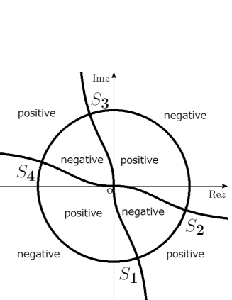
Figure 1: Signs of $\mathrm{Re\,}\varphi$

Let $\delta(z)$, analytic in $|z|\neq 1$, be the solution to the Riemann-Hilbert problem

$$\delta_{+}(z)=\delta_{-}(z)(1-|r(z)|^{2})\;\mbox{ on}\,\mathrm{arc}(S_{1}S_{2})\;\mbox{and}\;\mathrm{arc}(S_{3}S_{4}),$$ (31)

$$\delta_{+}(z)=\delta_{-}(z)\;\mbox{ on}\,\mathrm{arc}(S_{2}S_{3})\;\mbox{and}\;\mathrm{arc}(S_{4}S_{1}),$$ (32)

$$\delta(z)\to 1\;\mbox{ as}\;z\to\infty,$$ (33)

where $\mathrm{arc}(S_{j}S_{k})$ is the minor arc $\subset C$ joining $S_{j}$ and $S_{k}$ and the outside of $C$ is the plus side. On the singular locus $\mathrm{arc}(S_{1}S_{2})\cup\mathrm{arc}(S_{3}S_{4})$, $\delta_{\pm}(z)$ are the boundary values from $\pm\mathrm{Re\,}\varphi>0$ respectively, and there is no distinction between them on $\mathrm{arc}(S_{2}S_{3})\cup\mathrm{arc}(S_{4}S_{1})$.

This problem can be uniquely solved by the formula

$$\delta(z)=\exp\left(\frac{-1}{2\pi i}\left[\int_{S_{1}}^{S_{2}}+\int_{S_{3}}^{S_{4}}\right](\tau-z)^{-1}\log(1-|r(\tau)|^{2})\,d\tau\right),$$ (34)

where the contours are the arcs $\subset C$. We have $\delta(-z)=\delta(z)$ and $\delta^{\prime}(0)=0$ because $r(-\tau)=-r(\tau)$.

Conjugating our original Riemann-Hilbert problem (15)-(17) by

$$\Delta(z)=\begin{bmatrix}\delta(z)&\quad 0\\ 0&\quad\delta^{-1}(z)\end{bmatrix}=\delta^{\sigma_{3}}(z)$$

leads to the factorization problem for $m\Delta^{-1}$,

$$(m\Delta^{-1})_{+}(z)=(m\Delta^{-1})_{-}(z)(\Delta_{-}v\Delta_{+}^{-1}),\quad z\in C,$$ (35)

$$m\Delta^{-1}\to I\quad(z\to\infty).$$ (36)

Now, we rewrite (35)-(36) by choosing the counterclockwise orientation (the inside being the plus side) on $\mathrm{arc}(S_{2}S_{3})$ and $\mathrm{arc}(S_{4}S_{1})$ and the clockwise orientation (the outside being the plus side) on $\mathrm{arc}(S_{1}S_{2})$ and $\mathrm{arc}(S_{3}S_{4})$. The circle $|z|=1$ with this new orientation is denoted by $\widetilde{C}$ and the new Riemann-Hilbert problem on it is

$$(m\Delta^{-1})_{+}(z)=(m\Delta^{-1})_{-}(z)\tilde{v},\quad z\in\widetilde{C},$$ (37)

$$m\Delta^{-1}\to I\quad(z\to\infty),$$ (38)

for the 2$\times$2 matrix $\tilde{v}$. We have, by (31) and (32),

$$\tilde{v} =e^{-\varphi\mathrm{ad}\sigma_{3}}\left(\begin{bmatrix}1&\;0\\ r\delta_{-}^{-2}/(1-|r|^{2})\;&\;1\end{bmatrix}\begin{bmatrix}1\;&\;-\bar{r}\delta_{+}^{2}/(1-|r|^{2})\\ 0\;&\;1\end{bmatrix}\right) \mbox{ on }S_{1}S_{2}\cup S_{3}S_{4},$$

$$=e^{-\varphi\mathrm{ad}\sigma_{3}}\left(\begin{bmatrix}1\;&\;0\\ -r\delta^{-2}\;&\;1\end{bmatrix}\begin{bmatrix}1\;&\;\bar{r}\delta^{2}\\ 0\;&\;1\end{bmatrix}\right) \mbox{ on }S_{2}S_{3}\cup S_{4}S_{1}.$$

Set

$$\rho =-\bar{r}/(1-|r|^{2}) \mbox{\quad on\;}S_{1}S_{2}\cup S_{3}S_{4},$$ (39)

$$=\bar{r} \mbox{\quad on\;}S_{2}S_{3}\cup S_{4}S_{1},$$ (40)

then $\tilde{v}$ admits a unified expression

$$\tilde{v}=e^{-\varphi\mathrm{ad}\sigma_{3}}\left(\begin{bmatrix}1\;&\;0\\ -\bar{\rho}\delta_{-}^{-2}\;&\;1\end{bmatrix}\begin{bmatrix}1\;&\;\rho\delta_{+}^{2}\\ 0\;&\;1\end{bmatrix}\right)$$

on any of the arcs, where $\delta_{+}=\delta_{-}=\delta$ on $S_{2}S_{3}\cup S_{4}S_{1}$. We have a lower/upper factorization

$$\tilde{v} =b_{-}^{-1}b_{+},$$ (41)

$$b_{+} :=\delta_{+}^{\mathrm{ad}\sigma_{3}}e^{-\varphi\mathrm{ad}\sigma_{3}}\begin{bmatrix}1\;&\;\rho\\ 0\;&\;1\end{bmatrix}=\begin{bmatrix}1\;&\;\delta_{+}^{2}e^{-2\varphi}\rho\\ 0\;&\;1\end{bmatrix},\;$$ (42)

$$b_{-} :=\delta_{-}^{\mathrm{ad}\sigma_{3}}e^{-\varphi\mathrm{ad}\sigma_{3}}\begin{bmatrix}1\;&\;0\\ \bar{\rho}\;&\;1\end{bmatrix}=\begin{bmatrix}1\;&\;0\\ \delta_{-}^{-2}e^{2\varphi}\bar{\rho}\;&\;1\end{bmatrix}.$$ (43)

Later we shall use $w_{\pm}=\pm(b_{\pm}-I)$.

5 Decomposition, analytic continuation and estimates

From now on we assume $0<n\leq(2-V_{0})t$ so that $-\pi/4<\arg A<0$. Minor modifications are required in the construction of the contour $\Sigma$ (Figure 2 below) if $-(2-V_{0})t\leq n\leq 0$. See Remark 6.1.

Set

$$\psi=\varphi/(it)=2^{-1}(z-z^{-1})^{2}+int^{-1}\log z.$$

It is real-valued on $|z|=1$. For $z=e^{i\theta}\,(\theta\in\mathbb{R})$, we have $\psi=\cos 2\theta-nt^{-1}\theta-1$ and $\psi$ is monotone on any of $S_{1}S_{2}$, $S_{2}S_{3}$, $S_{3}S_{4}$, $S_{4}S_{1}$. The monotonicity also follows from the fact that there are no other stationary points of $\varphi$ on $|z|=1$ than $S_{j}$’s.

5.1 Decomposition on an arc and some estimates

We seek a decomposition $\rho=R+h_{I}+h_{II}$ with each term having a certain estimate. Set $\vartheta=\theta+\pi/4$, $\vartheta_{0}=\arg\bar{A}=\arctan\sqrt{(2t-n)/(2t+n)}$. Then $\mathrm{arc}(S_{1}S_{2})$ corresponds to $-\vartheta_{0}\leq\vartheta\leq\vartheta_{0}$. We regard the function $\rho$ on $\mathrm{arc}(S_{1}S_{2})$ as a function in $\vartheta$ and denote it by $\rho(\vartheta)$ by abuse of notation. We have $\rho(\vartheta)=H_{e}(\vartheta^{2})+\vartheta H_{o}(\vartheta^{2})\,(-\vartheta_{0}\leq\vartheta\leq\vartheta_{0})$ for smooth functions $H_{e}$ and $H_{o}$. By Taylor’s theorem, they are expressed as follows:

$$H_{e}(\vartheta^{2})=\mu_{0}^{e}+\cdots+\mu_{k}^{e}(\vartheta^{2}-\vartheta_{0}^{2})^{k}+\frac{1}{k!}\int_{\vartheta_{0}^{2}}^{\vartheta^{2}}H_{e}^{(k+1)}(\gamma)(\vartheta^{2}-\gamma)^{k}\,d\gamma,$$

$$H_{o}(\vartheta^{2})=\mu_{0}^{o}+\cdots+\mu_{k}^{o}(\vartheta^{2}-\vartheta_{0}^{2})^{k}+\frac{1}{k!}\int_{\vartheta_{0}^{2}}^{\vartheta^{2}}H_{o}^{(k+1)}(\gamma)(\vartheta^{2}-\gamma)^{k}\,d\gamma.$$

Here $k$ can be any positive integer, but we assume $k=4q+1,\,q\in\mathbb{Z}_{+}$ for convenience of later calculations.

We set

$$R(\vartheta) =R_{k}(\vartheta)=\sum_{i=0}^{k}\mu_{i}^{e}(\vartheta^{2}-\vartheta_{0}^{2})^{i}+\vartheta\sum_{i=0}^{k}\mu_{i}^{o}(\vartheta^{2}-\vartheta_{0}^{2})^{i},$$

$$\alpha(z) =(z-S_{1})^{q}(z-S_{2})^{q},$$

$$h(\vartheta) =\rho(\vartheta)-R(\vartheta)$$

and, by abuse of notation,

$$\alpha(\vartheta)=\alpha(e^{i(\vartheta-\pi/4)})=[e^{i(\vartheta-\pi/4)}-e^{i(-\vartheta_{0}-\pi/4)}]^{q}[e^{i(\vartheta-\pi/4)}-e^{i(\vartheta_{0}-\pi/4)}]^{q}.$$

Notice that we have $R(\pm\vartheta_{0})=\rho(\pm\vartheta_{0})$. The function $R$ extends analytically from $\mathrm{arc}(S_{1}S_{2})$ to a fairly large complex neighborhood. Its singularity comes only from that of $\log z$. By abuse of notation, $R(z)$ denotes the analytic function thus obtained, so that $R(\vartheta)=R(e^{i(\vartheta-\pi/4)})$ and $R(S_{j})=\rho(S_{j})$.

We have $\,d\psi/\,d\vartheta=2\cos 2\vartheta-n/t$ and it has a zero of order 1 at $\vartheta=\pm\vartheta_{0}$. Since $[-\vartheta_{0},\vartheta_{0}]\ni\vartheta\mapsto\psi\in\mathbb{R}$ is strictly increasing, we can consider its inverse $\vartheta=\vartheta(\psi)$, $\psi(-\vartheta_{0})\leq\psi\leq\psi(\vartheta_{0})$. We set

$$(h/\alpha)(\psi) =h(\vartheta(\psi))/\alpha(\vartheta(\psi)) \mbox{in}\;\psi(-\vartheta_{0})\leq\psi\leq\psi(\vartheta_{0}),$$

$$=0 \mbox{otherwise}.$$

Then $(h/\alpha)(\psi)$ is well-defined for $\psi\in\mathbb{R}$, and it can be shown that $h/\alpha\in H^{(3q+2)/2}(-\infty<\psi<\infty)$ and that its norm is uniformly bounded with respect to $(n,t)$ with (20). This argument is a ‘curved’ version of [10, (1.33)]. Notice that $\vartheta_{0}$, the counterpart of $z_{0}$ of [10], is trivially bounded.

Set

$$(\widehat{h/\alpha})(s)=\int_{-\infty}^{\infty}e^{-is\psi}(h/\alpha)(\psi)\frac{\,d\psi}{\sqrt{2\pi}},$$

$$h_{I}(\vartheta)=\alpha(\vartheta)\int_{t}^{\infty}e^{is\psi(\vartheta)}(\widehat{h/\alpha})(s)\frac{\,ds}{\sqrt{2\pi}},$$

$$h_{II}(\vartheta)=\alpha(\vartheta)\int_{-\infty}^{t}e^{is\psi(\vartheta)}(\widehat{h/\alpha})(s)\frac{\,ds}{\sqrt{2\pi}},$$

then $h(\vartheta)=h_{I}(\vartheta)+h_{II}(\vartheta)$, $|\vartheta|\leq\vartheta_{0}$ and

$$|e^{-2it\psi}h_{I}(\vartheta)|\leq C/t^{(3q+1)/2}$$ (44)

for some $C>0$ on $\mathrm{arc}(S_{1}S_{2})$. See [10, (1.36)]. The symbol $C$ always denotes a generic positive constant.

Set $p=\sqrt{2(2t-n)}/(\sqrt{2t+n\,}-\sqrt{2t-n\,}\,)>0$. We consider the contour $L_{12}=l_{12}\cup l_{21}\subset\{\mathrm{Re\,}\varphi\geq 0\}=\{\mathrm{Re\,}i\psi\geq 0\}$, where

$$l_{12}\colon z(u)=S_{1}+(p-u)A \;(0\leq u\leq p),$$

$$l_{21}\colon z(u)=S_{2}-iu\bar{A} \;(0\leq u\leq p).$$

We have chosen $p$ so that $S_{1}+pA=S_{2}-ip\bar{A}$, that is, $l_{12}$ and $l_{21}$ are joined at a single point.

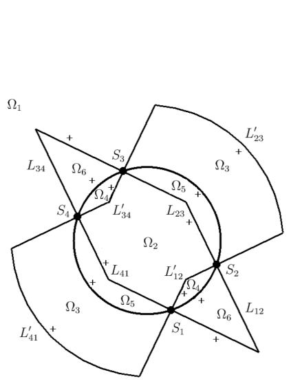
Figure 2: the contour $\Sigma$

We can show that $h_{II}(\vartheta)$ can be analytically continued to $\{\mathrm{Re\,}\varphi>0\}=\{\mathrm{Re\,}i\psi>0\}$. The extension is denoted by $h_{II}(z)$ so that $h_{II}(e^{i(\vartheta-\pi/4)})=h_{II}(\vartheta)$ by abuse of notation. On $l_{12}$, we have for $v=p-u(=$the distance from $S_{1})$,

$$|\alpha(z(u))|\leq v^{q}|S_{1}-S_{2}+vA|^{q}\leq C^{q}v^{q},$$

$$|e^{-2it\psi(z(u))}h_{II}(z(u))|\leq\frac{C^{q}v^{q}e^{-t\mathrm{Re\,}i\psi}}{\sqrt{2\pi}}\left(\int_{-\infty}^{t}\frac{\,ds}{1+s^{2}}\right)^{1/2}$$

$$\hskip 100.00015pt\times\left(\int_{-\infty}^{t}(1+s^{2})|(\widehat{h/\alpha})(s)|^{2}\,ds\right)^{1/2}.$$

We have

$$\mathrm{Re\,}i\psi\geq C^{\prime}v^{2}$$ (45)

for some $C^{\prime}>0$, because $v=0$ corresponds to the saddle point $S_{1}$. On $l_{12}$,

$$|e^{-2i\psi(z(u))}h_{II}(z(u))|\leq Cv^{q}e^{-C^{\prime}tv^{2}}=Ct^{-q/2}(tv^{2})^{q/2}e^{-C^{\prime}tv^{2}}\leq C/t^{q/2}.$$

We have a similar estimate on $l_{21}$. Therefore, all over $L_{12}$, we have

$$|e^{-2it\psi(z)}h_{II}(z)|\leq C/t^{q/2}.$$ (46)

For a small constant $\varepsilon>0$, let $l_{12}^{\varepsilon}\subset l_{12}$ and $l_{21}^{\varepsilon}\subset l_{21}$ be the segments given by

$$l_{12}^{\varepsilon}\colon z(u)=S_{1}+(p-u)A \quad(0\leq u\leq p-\varepsilon),$$

$$l_{21}^{\varepsilon}\colon z(u)=S_{2}-iu\bar{A} \quad(0<\varepsilon\leq u\leq p).$$

The segment $l^{\varepsilon}_{jk}$ is obtained by removing the $\varepsilon$-neighborhood of $S_{j}$ from $l_{jk}$. On $l_{12}^{\varepsilon}\cup l_{21}^{\varepsilon}\subset L_{12}$, we have $\mathrm{Re\,}i\psi\geq C_{\varepsilon}\varepsilon^{2}$ for some $C_{\varepsilon}>0$. It implies

$$|e^{-2it\psi(z)}R(z)|\leq Ce^{-C_{\varepsilon}\varepsilon^{2}t}.$$ (47)

5.2 Decomposition of another function on the same arc

The function $\bar{\rho}$ on $\mathrm{arc}(S_{1}S_{2})$ can be decomposed as $\bar{\rho}=\bar{R}+\bar{h}_{I}+\bar{h}_{II}$.

Set $p^{\prime}=\sqrt{2(2t-n)}/(\sqrt{2t+n\,}+\sqrt{2t-n\,}\,)>0$. We construct the contour $L^{\prime}_{12}=l^{\prime}_{12}\cup l^{\prime}_{21}$ in $\{\mathrm{Re\,}\varphi\leq 0\}=\{\mathrm{Re\,}i\psi\leq 0\}$ as follows:

$$l^{\prime}_{12}\colon z(u)=S_{1}+(p^{\prime}-u)iA \;(0\leq u\leq p^{\prime}),$$

$$l^{\prime}_{21}\colon z(u)=S_{2}-u\bar{A} \;(0\leq u\leq p^{\prime}).$$

We have chosen $p^{\prime}$ so that $l^{\prime}_{12}$ and $l^{\prime}_{21}$ are joined at a single point $S_{1}+ip^{\prime}A=S_{2}-p^{\prime}\bar{A}$.

In the same way as (44) and (46), we can show

$$|e^{2it\psi}\bar{h}_{I}(\vartheta)|\leq C/t^{(3q+1)/2}\;\mbox{ on}\;\mathrm{arc}(S_{1}S_{2}),$$ (48)

$$|e^{2it\psi(z)}\bar{h}_{II}(z)|\leq C/t^{q/2}\;\mbox{ on}\;L^{\prime}_{12}.$$ (49)

Set

$$l_{12}^{\prime\varepsilon}\colon z(u)=S_{1}+(p^{\prime}-u)iA \;(0\leq u\leq p^{\prime}-\varepsilon),$$

$$l_{21}^{\prime\varepsilon}\colon z(u)=S_{2}-u\bar{A} \;(\varepsilon\leq u\leq p^{\prime}).$$

In the same way as (47), we can show that

$$|e^{2it\psi(z)}\overline{R}(z)|\leq Ce^{-C_{\varepsilon}\varepsilon^{2}t}\;\mbox{on}\;l_{12}^{\prime\varepsilon}\cup l_{21}^{\prime\varepsilon}.$$ (50)

5.3 Decomposition on another arc

On $\mathrm{arc}(S_{2}S_{3})$, the functions $R,h_{I},h_{II},\bar{R},\bar{h}_{I},\bar{h}_{II}$ are constructed from $\rho$ and $\bar{\rho}$ in the same way as above. We have

$$|e^{-2it\psi}h_{I}|\leq C/t^{(3q+1)/2},\quad|e^{2it\psi}\bar{h}_{I}|\leq C/t^{(3q+1)/2}.$$

Set $p^{\prime\prime}=\sqrt{2(2t+n)}/(\sqrt{2t+n\,}+\sqrt{2t-n\,}\,)>0$. Let $L_{23}$ be the contour obtained by joining

$$l_{23}\colon z(u)=S_{2}+iu\bar{A} \quad(0\leq u\leq p^{\prime\prime}),$$

$$l_{32}\colon z(u)=S_{3}+(p^{\prime\prime}-u)A \quad(0\leq u\leq p^{\prime\prime}).$$

The segments $l_{jk}^{\varepsilon}\subset l_{jk},\,(j,k)=(2,3),(3,2)$ consist of points whose distance from $S_{j}$ is not less than $\varepsilon$. Notice that $S_{2}+ip^{\prime\prime}\bar{A}=S_{3}+p^{\prime\prime}A$ is inside the circle $|z|=1$. Then we can show in the same way as (46) and (47) that

$$|e^{-2it\psi(z)}h_{II}(z)|\leq C/t^{q/2}\quad\mbox{on }L_{23}.$$

$$|e^{-2it\psi(z)}R(z)|\leq Ce^{-C_{\varepsilon}\varepsilon^{2}t}\quad\mbox{on }l_{23}^{\varepsilon}\cup l_{32}^{\varepsilon}.$$

Next, let $L^{\prime}_{23}$ be the contour obtained by joining

$$l^{\prime}_{23}\colon z(u)=S_{2}+u\bar{A} (0\leq u\leq 1),$$

$$\hat{l}^{\prime}_{23}\colon z(u)=\mathrm{Arc}(S_{2}+\bar{A},S_{3}+iA),\;$$

$$l^{\prime}_{32}\colon z(u)=S_{3}+i(1-u)A (0\leq u\leq 1).$$

Here $\mathrm{Arc}(S_{2}+\bar{A},S_{3}+iA)$ is the minor arc $\subset\{|z|=(2+\sqrt{2})^{1/2}\}$ from $S_{2}+\bar{A}$ to $S_{3}+iA$. Then we have estimates on $l^{\prime}_{23}\cup l^{\prime}_{32}$ similar to (49). The arc $\hat{l}^{\prime}_{23}$ is away from the saddle points and we have exponential decay of $e^{2it\psi}\bar{h}_{II}$ on it. Therefore we get an estimate like (49) on $L^{\prime}_{23}$. Moreover, we obtain an estimate like (50) if we exclude the $\varepsilon$-neighborhood of $S_{2}$ and $S_{3}$.

5.4 Decomposition on the remaining arcs

We construct $L_{jk}$ and $L^{\prime}_{jk}$ for $(j,k)=(3,4),(4,1)$ by symmetry and get relevant estimates. The results in this section lead to Lemma 7.1 below.

6 A Riemann-Hilbert problem on a new contour

Set $L=\cup_{(j,k)}L_{jk}\subset\{\mathrm{Re\,}\varphi\geq 0\}$, $L^{\prime}=\cup_{(j,k)}L^{\prime}_{jk}\subset\{\mathrm{Re\,}\varphi\leq 0\}$, $\Sigma=\tilde{C}\cup L\cup L^{\prime}$. We define six open sets $\Omega_{1},\dots,\Omega_{6}$ as in Figure 2. The + signs indicate the plus sides of the curves. If $j$ is odd (resp. even), $\mathrm{arc}(S_{j}S_{j+1})$ is oriented clockwise (resp. counterclockwise) and $L\cup L^{\prime}$ is oriented inward (resp. outward) near $S_{j}$.

Remark 6.1.

If $n\leq 0$, the contour $\Sigma$ should be slightly modified.

1. If $n=0$, we should replace $L_{12}$ and $L_{23}$ with curves like $L^{\prime}_{23}$ and $L^{\prime}_{41}$ in Figure 2, each made up of two segments and an arc.

2. If $n$ is negative, the argument of $A$ is between $-\pi/4$ and $-\pi/2$. The parts $L^{\prime}_{23}$ and $L^{\prime}_{41}$ should each be made up of two segments, while $L_{12}$ and $L_{34}$ of two segments and an arc.

The expansion in Theorem 3.1 is uniform with respect to the ratio $n/t\in[-(2-V_{0}),2-V_{0}]$. The uniformity can be proved by considering the following three cases ($\epsilon>0$ is small): (a) $\epsilon\leq n/t\leq 2-V_{0}$, (b) $-\epsilon<n/t<\epsilon$, (c) $-(2-V_{0})\leq n/t\leq-\epsilon$. The uniformity in (a) follows from the calculations explicitly given in the present paper. The contour of the type in (i) [resp. (ii)] is useful in (b) [resp. (c)]. In dealing with each part of the contour, one has only to follow the subsection 5.1 (two segments) or 5.3 (two segments and an arc).

One can show the uniformity in $-(2-V_{0})\leq n/t\leq 2-V_{0}$ by using only one multipurpose contour of the type in (i). See Figure 3. We have chosen to use the contour as in Figure 2 in order to simplify the presentation in the case (a).

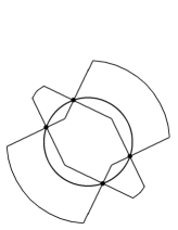
Figure 3: $\Sigma$ (multipurpose version)

Notice that each of $\Omega_{3},\dots,\Omega_{6}$ has two connected components and that $\Omega_{1}$ is unbounded. We introduce the following matrices:

$$b_{+}^{0}=\delta_{+}^{\mathrm{ad}\sigma_{3}}\rm e^{-\varphi\mathrm{ad}\sigma_{3}}\begin{bmatrix}1&\quad h_{I}\\ 0&\quad 1\end{bmatrix},\; b_{+}^{a}=\delta_{+}^{\mathrm{ad}\sigma_{3}}\rm e^{-\varphi\mathrm{ad}\sigma_{3}}\begin{bmatrix}1\;&\;h_{II}+R\\ 0\;&\;1\end{bmatrix},$$

$$b_{-}^{0}=\delta_{-}^{\mathrm{ad}\sigma_{3}}\rm e^{-\varphi\mathrm{ad}\sigma_{3}}\begin{bmatrix}1&\quad 0\\ \bar{h}_{I}&\quad 1\end{bmatrix},\; b_{-}^{a}=\delta_{-}^{\mathrm{ad}\sigma_{3}}\rm e^{-\varphi\mathrm{ad}\sigma_{3}}\begin{bmatrix}1\;&\;0\\ \bar{h}_{II}+\bar{R}\;&\;1\end{bmatrix}.$$

Then $b_{\pm}=b^{0}_{\pm}b^{a}_{\pm}$, $\tilde{v}=(b_{-}^{a})^{-1}(b_{-}^{0})^{-1}b_{+}^{0}b_{+}^{a}$. Define a new unknown matrix $m^{\sharp}$ by

$$m^{\sharp} =m\Delta^{-1}, z\in\Omega_{1}\cup\Omega_{2},$$ (51)

$$=m\Delta^{-1}(b_{-}^{a})^{-1}, z\in\Omega_{3}\cup\Omega_{4},$$ (52)

$$=m\Delta^{-1}(b_{+}^{a})^{-1}, z\in\Omega_{5}\cup\Omega_{6}.$$ (53)

By (37), (38) and (41) it is the unique solution to the Riemann-Hilbert problem

$$m^{\sharp}_{+}(z)=m^{\sharp}(z)_{-}v^{\sharp}(z), z\in\Sigma,$$ (54)

$$m^{\sharp}(z)\to I \mbox{as\;}z\to\infty.$$ (55)

Here $v^{\sharp}=v^{\sharp}(z)=v^{\sharp}(z;n,t)$ is defined by

$$v^{\sharp}(z) =(b_{-}^{0})^{-1}b_{+}^{0}, z\in\tilde{C},$$

$$=b_{+}^{a}, z\in L,$$

$$=(b_{-}^{a})^{-1}, \qquad z\in L^{\prime}.$$

Set $b^{\sharp}_{-}=b_{-}^{0},I,b_{-}^{a}$ and $b^{\sharp}_{+}=b_{+}^{0},b_{+}^{a},I$ on $\tilde{C},L,L^{\prime}$ respectively. Then, on $\Sigma$, we have

$$v^{\sharp}=v^{\sharp}(z)=(b_{-}^{\sharp})^{-1}b_{+}^{\sharp}.$$

In the next section, we shall employ $w_{\pm}^{\sharp}=\pm(b_{\pm}^{\sharp}-I)$, $w^{\sharp}=w_{+}^{\sharp}+w_{-}^{\sharp}$. We have $v^{\sharp}=(I-w^{\sharp}_{-})^{-1}(I+w^{\sharp}_{+})=(I+w^{\sharp}_{-})(I+w^{\sharp}_{+})$.

7 Reconstruction and a resolvent

7.1 Reconstruction

Since $\delta^{\prime}(0)=0$, (18) and (51) imply

$$R_{n}(t)=-\lim_{z\to 0}\frac{1}{z}(m^{\sharp}_{21}\delta)=-\frac{\,d}{\,dz}(m^{\sharp}_{21}\delta)\bigr{|}_{z=0}=-\delta(0)\frac{\,dm^{\sharp}_{21}}{\,dz}(0).$$ (56)

Let

$$(C_{\pm}f)(z)=\int_{\Sigma}\frac{f(\zeta)}{\zeta-z_{\pm}}\frac{\,d\zeta}{2\pi i},\;=\lim_{\genfrac{}{}{0.0pt}{}{z^{\prime}\to z}{z^{\prime}\in\{\pm\textrm{\scriptsize-side of }\Sigma\}}}\int_{\Sigma}\frac{f(\zeta)}{\zeta-z^{\prime}}\frac{\,d\zeta}{2\pi i},\;z\in\Sigma$$

be the Cauchy operators on $\Sigma$. Define $C_{w^{\sharp}}=C_{w^{\sharp}}^{\Sigma}\colon L^{2}(\Sigma)\to L^{2}(\Sigma)$ by

$$C_{w^{\sharp}}f=C_{w^{\sharp}}^{\Sigma}f=C_{+}(fw^{\sharp}_{-})+C_{-}(fw^{\sharp}_{+})$$ (57)

for a $2\times 2$ matrix-valued function $f$. Later we will define similar operators by replacing the pair $(\Sigma,w^{\sharp})$ with others. Even if a kernel, say $\omega_{\pm}$, is supported by a subcontour $\Sigma_{1}$ of $\Sigma_{2}$, it is necessary to distinguish between $C_{\omega}^{\Sigma_{1}}$ and $C_{\omega}^{\Sigma_{2}}$.

Let $\mu^{\sharp}$ be the solution to the equation

$$\mu^{\sharp}=I+C_{w^{\sharp}}\mu^{\sharp}.$$ (58)

Then we have $\mu^{\sharp}=(1-C_{w^{\sharp}})^{-1}I$ (the resolvent exists), and

$$m^{\sharp}(z;n,t)=I+\int_{\Sigma}\frac{\mu^{\sharp}(\zeta;n,t)w^{\sharp}(\zeta)}{\zeta-z}\frac{\,d\zeta}{2\pi i},\;z\in\mathbb{C}\setminus\Sigma$$ (59)

is the unique solution to the Riemann-Hilbert problem (54), (55). By substituting (59) into (56), we find that

$$\qquad R_{n}(t) =-\delta(0)\int_{\Sigma}\zeta^{-2}\left[\mu^{\sharp}(\zeta;n,t)w^{\sharp}(\zeta)\right]_{21}\frac{\,d\zeta}{2\pi i}$$ (60)

$$=-\delta(0)\int_{\Sigma}z^{-2}\left[\bigl{(}(1-C_{w^{\sharp}})^{-1}I\bigr{)}(z)w^{\sharp}(z)\right]_{21}\frac{\,dz}{2\pi i}.$$ (61)

In §9, we will prove that the resolvent $(1-C_{w^{\sharp}})^{-1}\colon L^{2}(\Sigma)\to L^{2}(\Sigma)$ indeed exists for any sufficiently large $t$ and that its norm is uniformly bounded.

7.2 Partition of the matrices

We set, for $0<\varepsilon<\inf_{(n,t)}p^{\prime}$,

$$\textstyle L_{\varepsilon} =\{z\in L;|z-S_{j}|>\varepsilon\;\mbox{for all}\;j=1,2,3,4\},$$

$$L^{\prime}_{\varepsilon} =\{z\in L^{\prime};|z-S_{j}|>\varepsilon\;\mbox{for all}\;j=1,2,3,4\}.$$

Set $w^{a}_{\pm}=w^{\sharp}_{\pm}|_{\tilde{C}}$ (consisting of quantities of type $h_{I}$ or $\bar{h}_{I}$ together with $\delta$ and $e^{\pm\varphi}=e^{\pm it\psi}$) on $\tilde{C}$ and $w^{a}_{\pm}=0$ on $\Sigma\setminus\tilde{C}$. Let $w^{b}_{\pm}$ be equal to the contribution to $w^{\sharp}_{\pm}$ from the quantities involving $h_{II}$ or $\bar{h}_{II}$ on $L\cup L^{\prime}$ and set $w^{b}_{\pm}=0$ on $\Sigma\setminus(L\cup L^{\prime})$. Additionally, let $w^{c}_{\pm}$ be equal to the contribution to $w^{\sharp}_{\pm}$ from the quantities involving $R$ or $\bar{R}$ on $L_{\varepsilon}\cup L^{\prime}_{\varepsilon}$ and set $w^{c}_{\pm}=0$ on $\Sigma\setminus(L_{\varepsilon}\cup L_{\varepsilon}^{\prime})$. Finally, we set $w^{e}_{\pm}=w^{a}_{\pm}+w^{b}_{\pm}+w^{c}_{\pm}$ and $w^{\prime}_{\pm}=w^{\sharp}_{\pm}-w^{e}_{\pm}$. These matrices are all upper or lower triangular and their diagonal elements are zero. We will show that $w_{\pm}^{e}$ are small in a certain sense and that the main contribution is by $w^{\prime}_{\pm}$.

We define $w^{*}=w^{*}_{+}+w^{*}_{-}$ for $*=a,b,c,e,^{\prime}$. Then we have $w^{e}=w^{a}+w^{b}+w^{c}$ and $w^{\prime}=w^{\sharp}-w^{e}$. Set $\Sigma^{\prime}=\{\Sigma\setminus(\tilde{C}\cup L_{\varepsilon}\cup L^{\prime}_{\varepsilon})\}\cup\{S_{1},S_{2},S_{3},S_{4}\}=(L\cup L^{\prime})\cap\cup_{j=1}^{4}\{|z-S_{j}|\leq\varepsilon\}$, then it is a union of four small crosses and $\mathrm{supp\,}w^{\prime}_{\pm}\subset\mathrm{supp\,}w^{\prime}\subset\Sigma^{\prime}$. As is shown in Figure 4, each cross is oriented inward or outward. We have

$$w^{\prime}_{+} =\delta^{\mathrm{ad\,}\sigma_{3}}e^{-\varphi{\mathrm{ad\,}\sigma_{3}}}\begin{bmatrix}0&\;R\\ 0&\;0\end{bmatrix}=\begin{bmatrix}0\;&\quad\delta^{2}e^{-2it\psi}R\\ 0\;&0\end{bmatrix} \quad\mbox{on\,}L\cap\Sigma^{\prime},$$ (62)

$$w^{\prime}_{-} =\delta^{\mathrm{ad\,}\sigma_{3}}e^{-\varphi{\mathrm{ad\,}\sigma_{3}}}\begin{bmatrix}0&\;0\\ -\bar{R}&\;0\end{bmatrix}=\begin{bmatrix}0&\quad 0\\ -\delta^{-2}e^{2it\psi}\bar{R}&\quad 0\end{bmatrix} \quad\mbox{on\,}L^{\prime}\cap\Sigma^{\prime}$$ (63)

and they vanish elsewhere.

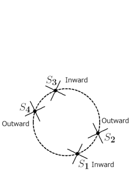
Figure 4: $\Sigma^{\prime}$: four small crosses

Lemma 7.1.

For any positive integer $\ell$, there exist positive constants $C$ and $\gamma_{\varepsilon}$ such that

$$|w^{a}_{\pm}|,\,|w^{a}|\leq Ct^{-\ell} \;\mbox{on}\;\tilde{C},$$ (64)

$$|w^{b}_{\pm}|,\,|w^{b}|\leq Ct^{-\ell} \;\mbox{on}\;L\cup L^{\prime},$$ (65)

$$|w^{c}_{\pm}|,\,|w^{c}|\leq Ce^{-\gamma_{\epsilon}t} \;\mbox{on}\;L_{\varepsilon}\cup L^{\prime}_{\varepsilon}.$$ (66)

$L^{p}$ estimates are easily obtained since the length of $\Sigma$ is bounded uniformly with respect to $(n,t)$ satisfying (20). Moreover we have

$$\|w^{\prime}_{\pm}\|_{L^{2}(\Sigma)}\leq Ct^{-1/4},\;\|w^{\prime}\|_{L^{2}(\Sigma)}\leq Ct^{-1/4},$$ (67)

$$\|w^{\prime}_{\pm}\|_{L^{1}(\Sigma)}\leq Ct^{-1/2},\;\|w^{\prime}\|_{L^{1}(\Sigma)}\leq Ct^{-1/2}.$$ (68)

Proof.

The boundedness of $\delta$ and $\delta^{-1}$ will be proved in §8. The inequality (64) follows from (44), (48) and their analogues. The inequalities (65) and (66) are consequences of (46), (47), (49), (50) and their analogues. Finally in order to derive (67) and (68), we employ (45) and its analogues. Since $R,\bar{R},\delta,\delta^{-1}$ are bounded, we have only to calculate the Gauss type integral $\int_{0}^{\infty}e^{-{\textrm{\scriptsize const.}}tv^{2}}\,dv$. ∎

We define the integral operators $C_{w^{\prime}}$ and $C_{w^{e}}$ from $L^{2}(\Sigma)$ to itself of the type (57). We have $C_{w^{\sharp}}=C_{w^{\prime}}+C_{w^{e}}$.

Later in §9 we will prove that $(1-C_{w^{\prime}})^{-1}$ and $(1-C_{w^{\sharp}})^{-1}$ exist and are uniformly bounded for any sufficiently large $t$. We proceed assuming this assertion.

7.3 Resolvents and estimates

By the second resolvent identity, or rather by (73) below, we get

$$\int_{\Sigma}z^{-2}\bigl{(}(1-C_{w^{\sharp}})^{-1}I\bigr{)}(z)w^{\sharp}(z)$$

$$=\int_{\Sigma}z^{-2}\bigl{(}(1-C_{w^{\prime}})^{-1}I\bigr{)}(z)w^{\prime}(z)+\mathrm{I}+\mathrm{II}+\mathrm{III}+\mathrm{IV},$$ (69)

where

$$\mathrm{I}=\int_{\Sigma}z^{-2}w^{e},\quad\mathrm{II}=\int_{\Sigma}z^{-2}(1-C_{w^{\prime}})^{-1}(C_{w^{e}}I)w^{\sharp},$$

$$\mathrm{III}=\int_{\Sigma}z^{-2}(1-C_{w^{\prime}})^{-1}(C_{w^{\prime}}I)w^{e},$$

$$\mathrm{IV}=\int_{\Sigma}z^{-2}(1-C_{w^{\prime}})^{-1}C_{w^{e}}(1-C_{w^{\sharp}})^{-1}(C_{w^{\sharp}}I)w^{\sharp}.$$

Since $|z^{-2}|$ is uniformly bounded on $\Sigma$, (64), (65) and (66) imply

$$|\mathrm{I}|,|\mathrm{II}|,|\mathrm{III}|,|\mathrm{IV}|\leq Ct^{-\ell}\quad\mbox{as}\;t\to\infty.$$ (70)

Proposition 7.2.

We have

$$R_{n}(t)=-\delta(0)\int_{\Sigma}z^{-2}\left[\bigl{(}(1-C_{w^{\prime}})^{-1}I\bigr{)}(z)w^{\prime}(z)\right]_{21}\frac{\,dz}{2\pi i}+O(t^{-\ell}).$$ (71)

Proof.

Use (61), (69) and (70). ∎

Proposition 7.3.

We have

$$R_{n}(t)=-\delta(0)\int_{\Sigma^{\prime}}z^{-2}\left[\bigl{(}(1-C_{w^{\prime}}^{\Sigma^{\prime}})^{-1}I\bigr{)}(z)w^{\prime}(z)\right]_{21}\frac{\,dz}{2\pi i}+O(t^{-\ell}).$$ (72)

Here $C_{w^{\prime}}^{\Sigma^{\prime}}$ is an integral operator on $L^{2}(\Sigma^{\prime})$ whose kernel is $w^{\prime}_{\pm}|_{\Sigma^{\prime}}$. Notice that $C_{w^{\prime}}$ is an integral operator on $L^{2}(\Sigma)$ whose kernel is $w^{\prime}_{\pm}$, matrices of functions on $\Sigma\supset\Sigma^{\prime}$.

Proof.

Since $\mathrm{supp}\,w^{\prime}_{\pm}\subset\Sigma^{\prime}$, we can replace $\int_{\Sigma}$ by $\int_{\Sigma^{\prime}}$. Apply [10, (2.61)]. ∎

Remark 7.4.

In deriving (69), we used the following formula: if the operators $A,B,C$ and the matrices $f,g,h$ are such that $A=B+C,f=g+h$, then

$${}\{(1-A)^{-1}I\}f =\{(1-B)^{-1}I\}g+h+\{(1-B)^{-1}(CI)\}f$$

$$\quad+\{(1-B)^{-1}(BI)\}h+\{(1-B)^{-1}C(1-A)^{-1}(AI)\}f.$$ (73)

In (69), $f,g,h$ involve the factor $z^{-2}$, which is absent in the calculation of [10]. Its presence complicates matters, and it will be dealt with in (98).

8 Saddle points and scaling operators

8.1 Some functions characterizing arcs and their boundedness

Set $T_{1}=T_{2}=e^{-\pi i/4}$, $T_{3}=T_{4}=e^{3\pi i/4}$ and

$$\chi_{j}(z)=\frac{1}{2\pi i}\int_{T_{j}}^{S_{j}}\log\frac{1-|r(\tau)|^{2}}{1-|r(S_{j})|^{2}}\frac{\,d\tau}{\tau-z},$$ (74)

$$\ell_{j}(z)=\int_{T_{j}}^{S_{j}}\frac{\,d\tau}{\tau-z},$$ (75)

$$\nu_{j}=-\frac{1}{2\pi}\log(1-|r(S_{j})|^{2})\geq 0$$ (76)

for $j=1,2,3,4$. The integral $\int_{T_{j}}^{S_{j}}$ is performed along the minor arc from $T_{j}$ to $S_{j}$, which we denote by $\mathrm{arc}(T_{j}S_{j})$. The integral $\chi_{j}(S_{j})$ is well-defined because the logarithm vanishes at $S_{j}$. Moreover, $\chi_{j}$ and $\ell_{j}$ are analytic in the complement of $\mathrm{arc}(T_{j}S_{j})$, in particular near $S_{k}\,(k\neq j)$. We have $\nu_{1}=\nu_{3},\nu_{2}=\nu_{4}$ and

$$\frac{1}{2\pi i}\int_{T_{j}}^{S_{j}}\log(1-|r(\tau)|^{2})\frac{\,d\tau}{\tau-z}=i\nu_{j}\ell_{j}(z)+\chi_{j}(z).$$ (77)

Set

$$\delta_{j}(z) =\exp\Bigl{(}(-1)^{j-1}(i\nu_{j}\ell_{j}(z)+\chi_{j}(z))\Bigr{)}$$ (78)

$$=\left(\frac{z-S_{j}}{z-T_{j}}\right)^{(-1)^{j-1}i\nu_{j}}e^{(-1)^{j-1}\chi_{j}(z)},$$ (79)

where $w^{i\nu_{j}}$ is cut along $\mathbb{R}_{-}$ and is positive on $\mathbb{R}_{+}$. It is analytic in the complement of $\mathrm{arc}(T_{j}S_{j})$ and satisfies a Riemann-Hilbert problem similar to (31)-(33). The function $\delta(z)$ in (34) is decomposed as

$$\delta(z)=\prod_{j=1}^{4}\delta_{j}(z).$$

Since $\mathrm{Im\,}\ell_{j}(z)=\arg[(z-S_{j})/(z-T_{j})]$, we see that $\exp(\pm i\nu_{j}\ell_{j}(z))$ is bounded. Let $V_{j},U_{j}\subset\mathrm{arc}(T_{j}S_{j})$ be sufficiently small neighborhoods of $T_{j}$ and $S_{j}$ respectively. Then $\chi_{j}(z)$ and its boundary values on $\mathrm{arc}(T_{j}S_{j})\setminus\{U_{j},V_{j}\}$ are bounded as is proved by the Plemelj formula ([1, 2]). This formula involves a principal value integral. Its boundedness in $U_{j}\setminus\{S_{j}\}$ (as $z$ approaches $S_{j}$) is derived from the above-mentioned fact that the logarithm in (74) vanishes at $\tau=S_{j}$.

The well-definedness of $\chi_{j}(S_{j})$ has been explained above. The points $T_{j}$’s have been chosen just for simplicity, not for necessity, and can be replaced by any other points on $\mathrm{arc}(S_{1}S_{2})$ or $\mathrm{arc}(S_{3}S_{4})$ (it results in another decomposition of $\delta$). Since there is nothing special about them as far as the product $\delta(z)$ is concerned, it is well-defined and bounded on each $V_{j}$. Hence $\delta(z)$, $\delta^{-1}(z)$ and their boundary values are bounded everywhere.

Remark 8.1.

If $j\neq k$, then $r(-\tau)=-r(\tau)$ implies $\chi_{j+2}(S_{j+2})=\chi_{j}(S_{j})$,   $\delta_{j+2}(S_{k+2})=\delta_{j}(S_{k})$ for $j=1,2$ and $k=1,2,3,4$ with the convention $S_{5}=S_{1},S_{6}=S_{2}$.

8.2 Scaling operators

In a neighborhood of each saddle point $S_{j}$, we have

$$\varphi(z)=\varphi(S_{j})+\frac{\varphi^{\prime\prime}(S_{j})}{2}(z-S_{j})^{2}+\varphi_{j}(z),\quad\varphi_{j}(z)=O(|z-S_{j}|^{3})$$ (80)

for some function $\varphi_{j}(z)$. Set

$$\beta_{j}=(-1)^{j}2^{-1}i(4t^{2}-n^{2})^{-1/4}S_{j}$$

so that $\varphi^{\prime\prime}(S_{j})\beta_{j}^{2}=(-1)^{j-1}i/2$. See (82).

Let the infinite crosses $\Sigma(S_{j})$’s and $\Sigma(0)_{j}$’s be defined by

$$\Sigma(S_{j}) =(S_{j}+A\mathbb{R})\cup(S_{j}+iA\mathbb{R}),\;\mbox{oriented inward } \;(j=1,3),$$

$$=(S_{j}+\bar{A}\mathbb{R})\cup(S_{j}+i\bar{A}\mathbb{R}),\;\mbox{oriented outward } \;(j=2,4),$$

$$\Sigma(0)_{j} =e^{\pi i/4}\mathbb{R}\cup e^{-\pi i/4}\mathbb{R},\;\mbox{oriented inward } \;(j=1,3),$$

$$=\mbox{the same set as above, }\;\mbox{oriented outward } \;(j=2,4).$$

Note that $\Sigma(S_{j})$ is obtained by extending one of the four small crosses forming $\Sigma^{\prime}$ and that the cut of $\delta_{j}$, namely $\mathrm{arc}(S_{j}T_{j})$, is between two rays of $\Sigma(S_{j})$.

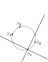
Figure 5: $\Sigma(S_{1})$: an infinite cross

We introduce the scaling operators with rotation

$$N_{j}\colon (\mathcal{C}^{0}\cup L^{2})(\Sigma(S_{j}))\to(\mathcal{C}^{0}\cup L^{2})(\Sigma(0)_{j}),\quad$$

$$f(z)\mapsto(N_{j}f)(z)=f(\beta_{j}z+S_{j}).$$

It is the pull-back by the mapping $M_{j}\colon\Sigma(0)_{j}\to\Sigma(S_{j})$, $z\mapsto\beta_{j}z+S_{j}$. The real axis is mapped by $M_{j}$ to the tangent line of the circle at $S_{j}$. The positive imaginary axis is mapped to the outer ($j=1,3$) or inner ($j=2,4$) normal. Hence the singularity of $\delta(z)$ is, if seen through $M_{j}$, to the left of $0$ either $j$ is even or odd.

By (79) and (80) we have

$$(N_{j}\delta_{j})(z) =\left(\frac{\beta_{j}z}{\beta_{j}z+S_{j}-T_{j}}\right)^{(-1)^{j-1}i\nu_{j}}e^{(-1)^{j-1}N_{j}\chi_{j}(z)}$$

$$=\left(\frac{\beta_{j}}{S_{j}-T_{j}}\right)^{(-1)^{j-1}i\nu_{j}}z^{(-1)^{j-1}i\nu_{j}}\left(\frac{S_{j}-T_{j}}{\beta_{j}z+S_{j}-T_{j}}\right)^{(-1)^{j-1}i\nu_{j}}$$

$$\hskip 15.00002pt\times e^{(-1)^{j-1}\chi_{j}(S_{j})}e^{(-1)^{j-1}\{N_{j}\chi_{j}(z)-\chi_{j}(S_{j})\}}.$$ (81)

$$(N_{j}e^{-\varphi})(z) =S_{j}^{n}e^{-it(S_{j}-S_{j}^{-1})^{2}/2}e^{(-1)^{j}iz^{2}/4}e^{-(N_{j}\varphi_{j})(z)}.$$ (82)

Here the arguments of $\beta_{j}/(S_{j}-T_{j})$ and of $(S_{j}-T_{j})/(\beta_{j}z+S_{j}-T_{j})$ (at least for a large positive $z$) are between $-\pi/2$ and $\pi/2$.

Originally, $N_{j}\delta_{j}$ has a cut along the preimage under $M_{j}$ of $\mathrm{arc}(S_{j}T_{j})$. It is an arc with central angle not exceeding $\pi/4$ which is tangent to the real line at the endpoint $0=M_{j}^{-1}(S_{j})$. See Figure 6. It is in the region $\pi\leq\arg z\leq 5\pi/4$ (if $j$ is odd) or $3\pi/4\leq\arg z\leq\pi$ (if $j$ is even). The factor $z^{i\nu_{j}}$ is originally cut along the union of the preimage and the half-line $C_{j}\colon z(u)=\beta_{j}^{-1}(-S_{j}+T_{j})-u,u\in\mathbb{R}_{+}$. See Figure 6. Since we consider $z^{i\nu_{j}}$ only on the cross $\Sigma(0)_{j}$, the cut can be moved homotopically as long as it is away from the cross. Hence the cut of $z^{i\nu_{j}}$ is moved to $\mathbb{R}_{-}$ for $j=1,2,3,4$. Another factor $\{(S_{j}-T_{j})/(\beta_{j}z+S_{j}-T_{j})\}^{i\nu_{j}}$ is cut along the half-line $C_{j}$, but its singularity eventually disappears as $t\to\infty,\beta_{j}\to 0$.

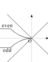
Figure 6: Cut of $N_{j}\delta_{j}$ and the cross

Set

$$\widehat{\delta}_{j}(z)=\delta(z)/\delta_{j}(z)=\prod_{k\neq j}\delta_{k}(z).$$ (83)

By (81) and (82), we have

$$N_{j}[\delta e^{-\varphi}]=N_{j}[\delta e^{-it\psi}](z)=\delta_{j}^{0}\delta_{j}^{1}(z),$$ (84)

where

$$\delta_{j}^{0}=S_{j}^{n}e^{-it(S_{j}-S_{j}^{-1})^{2}/2}\left(\frac{\beta_{j}}{S_{j}-T_{j}}\right)^{(-1)^{j-1}i\nu_{j}}e^{(-1)^{j-1}\chi_{j}(S_{j})}\widehat{\delta}_{j}(S_{j}),$$ (85)

$$\delta_{j}^{1}(z)=z^{(-1)^{j-1}i\nu_{j}}e^{(-1)^{j}iz^{2}/4}\left(\frac{S_{j}-T_{j}}{\beta_{j}z+S_{j}-T_{j}}\right)^{(-1)^{j-1}i\nu_{j}}$$

$$\hskip 50.00008pt\times e^{(-1)^{j-1}\{N_{j}\chi_{j}(z)-\chi_{j}(S_{j})\}-(N_{j}\varphi_{j})(z)}\frac{(N_{j}\widehat{\delta}_{j})(z)}{\widehat{\delta}_{j}(S_{j})}.$$ (86)

We choose the branch of the logarithm which is real on $\mathbb{R}_{+}$ and cut along $\mathbb{R}_{-}$. The imaginary powers in the definitions of $\delta^{0}_{j}$ and $\delta^{1}_{j}(z)$ should be interpreted accordingly. We have at least a pointwise convergence $\delta_{j}^{1}(z)\to z^{(-1)^{j-1}i\nu_{j}}e^{(-1)^{j}iz^{2}/4}$ as $t\to\infty$. In Proposition 10.1 we shall show that this convergence is uniform in a certain sense.

Remark 8.2.

We have $\hat{\delta}_{j+2}(S_{j+2})=\hat{\delta}_{j}(S_{j}),\;\delta_{j+2}^{0}=(-1)^{n}\delta_{j}^{0}\;(j=1,2)$ because of Remark 8.1. Since $T_{1}=T_{2}=\exp(-\pi i/4)$, the ratio $\beta_{j}/(S_{j}-T_{j})$ in the definition of $\delta^{0}_{j}$ can be represented by

$$\frac{\beta_{1}}{S_{1}-T_{1}}=\frac{-iA}{2(4t^{2}-n^{2})^{1/4}(A-1)},\quad\frac{\beta_{2}}{S_{2}-T_{2}}=\frac{i\bar{A}}{2(4t^{2}-n^{2})^{1/4}(\bar{A}-1)}.$$ (87)

These quantities are nothing but $D_{1}$ and $D_{2}$ in (25).

The cross $\Sigma(S_{j})$ is the union of the two lines $\Sigma(S_{j},L)$ and $\Sigma(S_{j},L^{\prime})$ defined by

$$\Sigma(S_{j},L) =S_{j}+e^{\pi i/4}S_{j}\mathbb{R}=S_{j}+A\mathbb{R} \quad(j=1,3),$$

$$=S_{j}+e^{-\pi i/4}S_{j}\mathbb{R}=S_{j}+i\bar{A}\mathbb{R} \quad(j=2,4),$$

$$\Sigma(S_{j},L^{\prime}) =S_{j}+e^{-\pi i/4}S_{j}\mathbb{R}=S_{j}+iA\mathbb{R} \quad(j=1,3),$$

$$=S_{j}+e^{\pi i/4}S_{j}\mathbb{R}=S_{j}+\bar{A}\mathbb{R} \quad(j=2,4).$$

Notice that each $\Sigma(S_{j},L)$ [resp. $\Sigma(S_{j},L^{\prime})$] share some segment with $L$ [resp. $L^{\prime}$], but is not included in it. We have $M_{j}^{-1}\Sigma(S_{j},L)=e^{-\pi i/4}\mathbb{R}\,(j=1,3)$, the direction of steepest descent of $e^{-iz^{2}/4}$, and $M_{j}^{-1}\Sigma(S_{j},L)=e^{\pi i/4}\mathbb{R}\,(j=2,4)$, the direction of steepest descent of $e^{iz^{2}/4}$. Therefore $\Sigma(S_{j},L)$ is in the direction of steepest descent of $e^{-\varphi}$ for any $j=1,2,3,4$ in view of (82). Similarly, $\Sigma(S_{j},L^{\prime})\,(j=1,2,3,4)$ is in the direction of steepest descent of $e^{\varphi}$.

We introduce some sets each of which is in a neighborhood of a saddle point. (In contrast, $L_{\varepsilon}$ and $L^{\prime}_{\varepsilon}$ to be introduced later are away from the saddle points. )

$$\Sigma(S_{j},L)_{\varepsilon} =\{z\in\Sigma(S_{j},L);|z-S_{j}|\leq\varepsilon\}\; \mbox{(a short segment)},$$

$$\Sigma(S_{j},L^{\prime})_{\varepsilon} =\{z\in\Sigma(S_{j},L^{\prime});|z-S_{j}|\leq\varepsilon\}\; \mbox{(another short segment)},$$

$$\Sigma(S_{j})_{\varepsilon} =\Sigma(S_{j},L)_{\varepsilon}\cup\Sigma(S_{j},L^{\prime})_{\varepsilon}\; \mbox{(a small cross)}.$$

Then $\Sigma(S_{j})_{\varepsilon}=\{z\in\Sigma(S_{j});\,|z-S_{j}|\leq\varepsilon\}$, $\Sigma^{\prime}=\cup_{j=1}^{4}\Sigma(S_{j})_{\varepsilon}$, $\mathrm{supp}\,w^{\prime}_{+}\subset\Sigma^{\prime}\cap L=\cup_{j=1}^{4}\Sigma(S_{j},L)_{\varepsilon}$ and $\mathrm{supp}\,w^{\prime}_{-}\subset\Sigma^{\prime}\cap L^{\prime}=\cup_{j=1}^{4}\Sigma(S_{j},L^{\prime})_{\varepsilon}$.

9 Crosses

Split $\Sigma^{\prime}$ into the union of four disjoint small crosses: $\Sigma^{\prime}=\cup_{j=1}^{4}\Sigma(S_{j})_{\varepsilon}$. We decompose $w^{\prime}_{\pm}$ into the form

$$w^{\prime}_{\pm}=\sum_{j=1}^{4}w^{j}_{\pm},$$ (88)

where $\mathrm{supp\,}w^{j}_{+}\subset\Sigma(S_{j},L)_{\varepsilon}$ and $\mathrm{supp\,}w^{j}_{-}\subset\Sigma(S_{j},L^{\prime})_{\varepsilon}$. Set $w^{j}=w^{j}_{+}+w^{j}_{-}$. Define the operators $A_{j}=C_{w^{j}}\,(j=1,2,3,4)$ on $L^{2}(\Sigma^{\prime})$ as in (57). We have $w^{\prime}=\sum_{j}w^{j}$ and $C_{w^{\prime}}^{\Sigma^{\prime}}=\sum_{j}A_{j}$. See Proposition 7.3 for the distinction between $C^{\Sigma^{\prime}}_{w^{\prime}}$ and $C_{w^{\prime}}$.

Lemma 9.1.

If $j\neq k$, we have

$$\|A_{j}A_{k}\|_{L^{2}(\Sigma^{\prime})}\leq Ct^{-1/2},\quad\|A_{j}A_{k}\|_{L^{\infty}(\Sigma^{\prime})\to L^{2}(\Sigma^{\prime})}\leq Ct^{-3/4}.$$ (89)

Proof.

Follow the proof of [10, Lemma 3.5]. Use Lemma 7.1 and the fact that $\mathrm{dist}(\Sigma(S_{j})_{\varepsilon},\Sigma(S_{k})_{\varepsilon})$ is bounded from below. ∎

In §11 we will prove the existence and boundedness of $(1-A_{j})^{-1}\colon L^{2}(\Sigma^{\prime})\to L^{2}(\Sigma^{\prime})\,(j=1,2,3,4)$. In view of Lemma 89 and [10, Lemma 3.15], it leads to that of $(1-C_{w^{\prime}}^{\Sigma^{\prime}})^{-1}\colon L^{2}(\Sigma^{\prime})\to L^{2}(\Sigma^{\prime})$. By [10, Lemma 2.56], we find that $(1-C_{w^{\prime}})^{-1}\colon L^{2}(\Sigma)\to L^{2}(\Sigma)$ exists and is bounded. Finally $(1-C_{w^{\sharp}})^{-1}\colon L^{2}(\Sigma)\to L^{2}(\Sigma)$ also exists and is bounded because of the smallness of $C_{w^{\sharp}}-C_{w^{\prime}}=C_{w^{e}}$ and the second resolvent identity $(1-A)^{-1}=\{(1-B)^{-1}(B-A)+1\}^{-1}(1-B)^{-1}$.

We have

$$\|A_{j}A_{k}(1-A_{k})^{-1}I\|_{L^{2}(\Sigma^{\prime})}$$

$$\leq\|A_{j}A_{k}I\|_{L^{2}(\Sigma^{\prime})}+\|A_{j}A_{k}(1-A_{k})^{-1}A_{k}I\|_{L^{2}(\Sigma^{\prime})}.$$ (90)

Here $\|A_{j}A_{k}I\|_{L^{2}(\Sigma^{\prime})}\leq Ct^{-3/4}$ follows from the second inequality of Lemma 89. On the other hand, we have $\|A_{k}I\|_{L^{2}(\Sigma^{\prime})}\leq\|w^{k}\|_{L^{2}(\Sigma^{\prime})}\leq\|w^{\prime}\|_{L^{2}(\Sigma^{\prime})}\leq Ct^{-1/4}$ by (67). This estimate, together with the first inequality of Lemma 89 and the boundedness of $(1-A_{j})^{-1}$, yields

$$\|A_{j}A_{k}(1-A_{k})^{-1}I\|_{L^{2}(\Sigma^{\prime})}\leq Ct^{-3/4}.$$ (91)

Following (repeatedly) [10, pp.338-339], we obtain by (91) and Lemma 89

$$\int_{\Sigma^{\prime}}z^{-2}\left((1-C_{w^{\prime}}^{\Sigma^{\prime}})^{-1}I\right)w^{\prime}$$

$$=\int_{\Sigma^{\prime}}z^{-2}\Bigl{(}\bigl{\{}{\textstyle 1+\sum_{j}A_{j}(1-A_{j})^{-1}}\bigr{\}}I\Bigr{)}w^{\prime}+O(t^{-1})$$

$$=\int_{\Sigma^{\prime}}z^{-2}w^{\prime}+\sum_{j,k=1}^{4}z^{-2}\left(A_{j}(1-A_{j})^{-1}I\right)w^{k}+O(t^{-1}).$$ (92)

We have sixteen quantities involving the pairs $(A_{j}(1-A_{j})^{-1},w^{k})\,(j,k\in\{1,2,3,4\})$. We claim that the main contribution is by the ‘diagonal’ pairs ($j=k$). Let us estimate the ‘off diagonal’ terms.

Since $(1-A_{j})^{-1}=1+(1-A_{j})^{-1}A_{j}$, we have

$$\biggl{|}\int_{\Sigma^{\prime}}z^{-2}\bigl{(}A_{j}(1-A_{j})^{-1}I\bigr{)}w^{k}\biggr{|}$$

$$\leq\biggl{|}\int_{\Sigma^{\prime}}z^{-2}(A_{j}I)w^{k}\biggr{|}+\biggl{|}\int_{\Sigma^{\prime}}z^{-2}\bigl{\{}A_{j}(1-A_{j})^{-1}A_{j}I\bigr{\}}w^{k}\biggr{|}.$$ (93)

Notice that the distance of $z\in\Sigma(S_{k})_{\varepsilon}$ and $\eta\in\Sigma(S_{j})_{\varepsilon}$ and that of $z\in\Sigma^{\prime}$ and $0$ are bounded from below. These facts, combined with (68), lead to the following Fubini type estimate of the iterated integral in the first term:

$$\biggl{|}\int_{\Sigma^{\prime}}z^{-2}(A_{j}I)w^{k}\biggr{|}=\biggl{|}\int_{\Sigma(S_{k})_{\varepsilon}}z^{-2}\biggl{(}\int_{\Sigma(S_{j})_{\varepsilon}}\frac{w^{j}(\eta)}{\eta-z}\frac{\,d\eta}{2\pi i}\biggr{)}w^{k}(z)\,dz\biggr{|}$$

$$\leq C\|w^{j}(\eta)\|_{L^{1}(\Sigma(S_{j})_{\varepsilon})}\|w^{k}(z)\|_{L^{1}(\Sigma(S_{k})_{\varepsilon})}\leq Ct^{-1}.$$ (94)

The second term in (93) is estimated in a slightly different way. By (67), (68) and the Schwarz inequality,

$$\biggl{|}\int_{\Sigma^{\prime}}z^{-2}\bigl{\{}A_{j}(1-A_{j})^{-1}A_{j}I\bigr{\}}w^{k}\biggr{|}$$

$$=\biggl{|}\int_{\Sigma(S_{k})_{\varepsilon}}\Bigl{\{}\int_{\Sigma(S_{j})_{\varepsilon}}\frac{\bigl{(}(1-A_{j})^{-1}A_{j}I\bigr{)}(\eta)w^{j}(\eta)}{\eta-z}\frac{\,d\eta}{2\pi i}\Bigr{\}}z^{-2}w^{k}(z)\biggr{|}$$

$$\leq C\|(1-A_{j})^{-1}A_{j}I\|_{L^{2}(\Sigma(S_{j})_{\varepsilon})}\|w^{j}(\eta)\|_{L^{2}(\Sigma(S_{j})_{\varepsilon})}\|z^{-2}w^{k}(z)\|_{L^{1}(\Sigma(S_{k})_{\varepsilon})}$$

$$\leq C\|w^{j}\|^{2}_{L^{2}(\Sigma(S_{j})_{\varepsilon})}\|w^{k}\|_{L^{1}(\Sigma(S_{k})_{\varepsilon})}\leq Ct^{-1}.$$ (95)

By using (92)-(95) and $w^{\prime}=\sum_{j=1}^{4}\left((1-A_{j})(1-A_{j})^{-1}I\right)w^{j}$, we get

$$\int_{\Sigma^{\prime}}z^{-2}\left((1-C_{w^{\prime}}^{\Sigma^{\prime}})^{-1}I\right)w^{\prime}=\sum_{j=1}^{4}\int_{\Sigma(S_{j})_{\varepsilon}}z^{-2}\bigl{[}(1-A_{j})^{-1}I\bigr{]}w^{j}+O(t^{-1}).$$

Owing to [10, (2.61)], $A_{j}=C_{w^{j}}\colon L^{2}(\Sigma^{\prime})\to L^{2}(\Sigma^{\prime})$ in the above formula can be replaced by $C^{\varepsilon}_{w^{j}}\colon L^{2}(\Sigma(S_{j})_{\varepsilon})\to L^{2}(\Sigma(S_{j})_{\varepsilon})$, which is defined as in (57) for the pair $(\Sigma(S_{j})_{\varepsilon},w^{j})$. Combining this fact with Proposition 7.3 ($\ell\geq 1$), we get the following result, which shows that the contributions of the four small crosses can be separated out.

Proposition 9.2.

We have

$${}\qquad R_{n}(t)=-\delta(0)\sum_{j=1}^{4}\int_{\Sigma(S_{j})_{\varepsilon}}z^{-2}\Bigl{[}\bigl{(}(1-C^{\varepsilon}_{w^{j}})^{-1}I\bigr{)}(z)w^{j}(z)\Bigr{]}_{21}\frac{\,dz}{2\pi i}+O(t^{-1}).$$

10 Infinite crosses and localization

We introduce $\hat{w}^{j}_{\pm}$ and $\hat{w}^{j}$ on the infinite cross $\Sigma(S_{j})$ given by

$$\hat{w}^{j}_{\pm} =w^{j}_{\pm},\quad z\in\Sigma(S_{j})_{\varepsilon},$$

$$\hat{w}^{j}_{\pm} =0,\quad z\in\Sigma(S_{j})\setminus\Sigma(S_{j})_{\varepsilon},$$

$$\hat{w}^{j} =\hat{w}^{j}_{+}+\hat{w}^{j}_{-},\quad z\in\Sigma(S_{j}).$$

Define the operator $\hat{A}_{j}\colon L^{2}(\Sigma(S_{j}))\to L^{2}(\Sigma(S_{j}))$ as in (57) with the kernel $\hat{w}^{j}_{\pm}$. Set $\Delta_{j}^{0}=(\delta_{j}^{0})^{\sigma_{3}},\,\tilde{\Delta}_{j}^{0}\phi=\phi\Delta_{j}^{0}$. The operator $\tilde{\Delta}_{j}^{0}$ and its inverse are bounded. Define $\alpha_{j}\colon L^{2}(\Sigma(0)_{j})\to L^{2}(\Sigma(0)_{j})$ by

$${}\qquad\alpha_{j} =C_{(\Delta_{j}^{0})^{-1}(N_{j}\hat{w}^{j})\Delta_{j}^{0}}$$

$$=C_{+}(\bullet\,(\Delta_{j}^{0})^{-1}(N_{j}\hat{w}^{j}_{-})\Delta_{j}^{0})+C_{-}(\bullet\,(\Delta_{j}^{0})^{-1}(N_{j}\hat{w}^{j}_{+})\Delta_{j}^{0}).$$ (96)

Then we have

$$\alpha_{j}=\tilde{\Delta}_{j}^{0}N_{j}\hat{A}^{j}N_{j}^{-1}(\tilde{\Delta}_{j}^{0})^{-1},\quad\hat{A}^{j}=N_{j}^{-1}(\tilde{\Delta}_{j}^{0})^{-1}\alpha_{j}\tilde{\Delta}_{j}^{0}N_{j}.$$ (97)

On $M_{j}^{-1}\Sigma(S_{j},L)_{\varepsilon}\setminus\{0\}\subset\Sigma(0)_{j}$, we have

$$\Bigl{(}(\Delta_{j}^{0})^{-1}(N_{j}[z^{-2}\hat{w}^{j}_{+}])\Delta_{j}^{0}\Bigr{)}(z)=\begin{bmatrix}0\quad&(\beta_{j}z+S_{j})^{-2}R(\beta_{j}z+S_{j})\delta_{j}^{1}(z)^{2}\\ 0\quad&0\end{bmatrix}$$

by (62), and the left-hand side is zero on $\Sigma(0)_{j}\setminus M_{j}^{-1}\Sigma(S_{j},L)_{\varepsilon}$.

On $M_{j}^{-1}\Sigma(S_{j},L^{\prime})_{\varepsilon}\subset\Sigma(0)_{j}$, we have

$$\Bigl{(}(\Delta_{j}^{0})^{-1}(N_{j}[z^{-2}\hat{w}^{j}_{-}])\Delta_{j}^{0}\Bigr{)}(z)=\begin{bmatrix}0\quad&0\\ -(\beta_{j}z+S_{j})^{-2}\bar{R}(\beta_{j}z+S_{j})\delta_{j}^{1}(z)^{-2}\quad&0\end{bmatrix}$$

by (63), and the left-hand side is zero on $\Sigma(0)_{j}\setminus M_{j}^{-1}\Sigma(S_{j},L^{\prime})_{\varepsilon}$.

Assume that $j$ is odd ($j=1,3$). We have $M_{j}^{-1}\Sigma(S_{j},L)_{\varepsilon}=e^{-\pi i/4}\mathbb{R}\cap\{|\beta_{j}z|\leq\varepsilon\}$ and it is the union of the lower right ($z/e^{-\pi i/4}\geq 0$) and upper left ($-z/e^{-\pi i/4}\geq 0$) parts. Recall that the positive imaginary axis is mapped by $M_{j}$ to the outer normal at $S_{j}$ if $j$ is odd.

Proposition 10.1.

Assume $j=1$ or $3$. Fix an arbitrary constant $\gamma$ with $0<2\gamma<1$. Then on $M_{j}^{-1}\Sigma(S_{j},L)_{\varepsilon}\cap\{z;\,\pm z/e^{-\pi i/4}>0\}$ respectively, we have

$$\Bigl{|}(\beta_{j}z+S_{j})^{-2}R(\beta_{j}z+S_{j})\delta_{j}^{1}(z)^{2}-S_{j}^{-2}R(S_{j}\pm)z^{2i\nu_{j}}e^{-iz^{2}/2}\Bigr{|}$$

$$\leq Ct^{-1/2}\log t\cdot\Bigl{|}e^{-\frac{i\gamma z^{2}}{2}}\Bigr{|},$$ (98)

$$\Bigl{|}R(\beta_{j}z+S_{j})\delta_{j}^{1}(z)^{2}-R(S_{j}\pm)z^{2i\nu_{j}}e^{-iz^{2}/2}\Bigr{|}$$

$$\leq Ct^{-1/2}\log t\cdot\Bigl{|}e^{-\frac{i\gamma z^{2}}{2}}\Bigr{|}.$$ (99)

We choose $R(S_{j}+)=\bar{r}(S_{j})$ on the lower right part and $R(S_{j}-)=-\bar{r}(S_{j})/(1-|r(S_{j})|^{2})$ on the upper left part. The analytic functions $z^{\pm 2i\nu_{j}}$ and $\delta^{1}_{j}(z)$ have cuts along $\mathbb{R}_{-}$.

Proof.

We show only (98) because (99) is just an easier version of it. Moreover we can assume $j=1$ by symmetry. On $M_{1}^{-1}\Sigma(S_{1},L)_{\varepsilon}$, we have

$$\Bigl{|}e^{\frac{i\gamma z^{2}}{2}}\Bigr{|}\Bigl{|}(\beta_{1}z+S_{1})^{-2}R(\beta_{1}z+S_{1})\delta_{1}^{1}(z)^{2}-S_{1}^{-2}R(S_{1}\pm)z^{2i\nu_{1}}e^{-iz^{2}/2}\Bigr{|}$$

$$\leq\Bigl{|}e^{-\frac{i\gamma z^{2}}{2}}\Bigl{[}R(\beta_{1}z+S_{1})\mathrm{F}\mathrm{E}_{1}\mathrm{E}_{2}\frac{N_{1}\hat{\delta}_{1}(z)^{2}}{\hat{\delta}_{1}(S_{1})^{2}}-S_{1}^{-2}R(S_{1}\pm)z^{2i\nu_{1}}e^{i(-1+2\gamma)\frac{z^{2}}{2}}\Bigr{]}\Bigr{|},$$ (100)

where

$$\mathrm{F} =(\beta_{1}z+S_{1})^{-2}\Bigl{(}\frac{S_{1}-T_{1}}{\beta_{1}z+S_{1}-T_{1}}\Bigr{)}^{2i\nu_{1}},$$ (101)

$$\mathrm{E}_{1} =z^{2i\nu_{1}}\exp\biggl{(}i(-1+2\gamma)\frac{z^{2}}{2}-2N_{1}\varphi_{1}(z)\biggr{)},$$ (102)

$$\mathrm{E}_{2} =\exp\Bigl{(}2\{N_{1}\chi_{1}(z)-\chi_{1}(S_{1})\}\Bigr{)}.$$ (103)

Each factor in (100) is uniformly bounded with respect to $(n,t)$.

Since $ze^{-i\gamma z^{2}/2}$ is bounded and $\beta_{1}=O(t^{-1/2})$, we have

$$\bigl{|}e^{-\frac{i\gamma z^{2}}{2}}\bigl{[}R(\beta_{1}z+S_{1})-R(S_{1}\pm)\bigr{]}\bigr{|}$$

$$\leq\bigl{|}e^{-\frac{i\gamma z^{2}}{2}}\bigr{|}|\beta_{1}z|\sup_{|w|\leq\varepsilon}|R^{\prime}(w+S_{1})|\leq C|\beta_{1}|\leq Ct^{-1/2}.$$ (104)

Similarly, we obtain

$$|e^{-\frac{i\gamma z^{2}}{2}}(F-S_{1}^{-2})|\leq Ct^{-1/2},$$ (105)

$$\biggl{|}e^{-\frac{i\gamma z^{2}}{2}}\biggl{[}\frac{N_{1}\hat{\delta}_{1}(z)^{2}}{\hat{\delta}_{1}(S_{1})^{2}}-1\biggr{]}\biggr{|}\leq Ct^{-1/2}.$$ (106)

Moreover, $N_{1}\varphi_{1}(z)=O(|\beta_{1}z|^{3})$ and the boundedness of $z^{2i\nu_{1}}$ and $z^{3}e^{-i\gamma z^{2}/2}$ imply

$$\left|e^{-i\gamma z^{2}/2}\left[\mathrm{E}_{1}-z^{2i\nu_{1}}\exp\left(i(-1+2\gamma)z^{2}/2\right)\right]\right|$$

$$\leq\left|e^{-i\gamma z^{2}/2}\right|\sup_{0\leq s\leq 1}\left|\frac{\,d}{\,ds}\exp\biggl{(}i(-1+2\gamma)\frac{z^{2}}{2}-2sN_{1}\varphi_{1}(z)\biggr{)}\right|$$

$$\leq C\left|e^{-i\gamma z^{2}/2}\right||\beta_{1}z|^{3}\leq C|\beta_{1}|^{3}\leq Ct^{-3/2}\leq Ct^{-1/2}.$$ (107)

Four $t^{-1/2}$ type estimates (104)-(107) have been obtained.

Lastly we derive a $t^{-1/2}\log t$ type estimate involving $E_{2}$. We have

$$\left|e^{-i\gamma z^{2}/2}(\mathrm{E}_{2}-1)\right|$$

$$\leq\sup_{0\leq s\leq 1}\left|e^{2s\{N_{1}\chi_{1}(z)-\chi_{1}(S_{1})\}}\right|\cdot\left|2e^{-i\gamma z^{2}/2}(N_{1}\chi_{1}(z)-\chi_{1}(S_{1}))\right|.$$ (108)

Since the supremum is bounded, we have only to derive a $t^{-1/2}\log t$ type estimate of the second factor in (108). Integration by parts yields

$$2\pi i[N_{1}\chi_{1}(z)-\chi_{1}(S_{1})]$$

$$=\int_{T_{1}}^{S_{1}}\log\frac{1-|r(\tau)|^{2}}{1-|r(S_{1})|^{2}}\,d\log\frac{\tau-(\beta_{1}z+S_{1})}{\tau-S_{1}}=-L_{1}-L_{2},$$ (109)

where

$$L_{1}=\log\frac{1-|r(T_{1})|^{2}}{1-|r(S_{1})|^{2}}\log\frac{T_{1}-(\beta_{1}z+S_{1})}{T_{1}-S_{1}},$$ (110)

$$L_{2}=\int_{T_{1}}^{S_{1}}\log\frac{\tau-(\beta_{1}z+S_{1})}{\tau-S_{1}}g(\tau)\,d\tau,$$ (111)

$$g(\tau)=\frac{\,d}{\,d\tau}\log(1-|r(\tau)|^{2}).$$ (112)

The first logarithm in $L_{1}$ is bounded. The second logarithm can be estimated in the same way as (104) etc. and we get

$$|e^{-i\gamma z^{2}/2}L_{1}|\leq Ct^{-1/2}.$$ (113)

We express the integral $L_{2}$ as the sum of two terms:

$$L_{2} =L_{2}^{1}+L_{2}^{2},$$

$$L_{2}^{1} =\int_{T_{1}}^{S_{1}}\{g(\tau)-g(S_{1})\}\log\frac{\tau-(\beta_{1}z+S_{1})}{\tau-S_{1}}\,d\tau,$$ (114)

$$L_{2}^{2} =g(S_{1})\int_{T_{1}}^{S_{1}}\log\frac{\tau-(\beta_{1}z+S_{1})}{\tau-S_{1}}\,d\tau.$$ (115)

We have $|\log(1+w)|=|\int_{0}^{w}(1+z)^{-1}\,\,dz|\leq C|w|$ in any sector that is away from the negative real axis. For $\tau$ and $z$ in $L_{2}^{1}$, the ratio $-\beta_{1}z/(\tau-S_{1})$ is in such a sector and

$$\left|\log\frac{\tau-(\beta_{1}z+S_{1})}{\tau-S_{1}}\right|=\left|\log\Bigl{(}1-\frac{\beta_{1}z}{\tau-S_{1}}\Bigr{)}\right|\leq C\left|\frac{\beta_{1}z}{\tau-S_{1}}\right|.$$ (116)

It implies

$${}\qquad|e^{-i\gamma z^{2}/2}L_{2}^{1}|\leq C|e^{-i\gamma z^{2}/2}||\beta_{1}z|\int_{T_{1}}^{S_{1}}\left|\frac{g(\tau)-g(S_{1})}{\tau-S_{1}}\right||\,d\tau|\leq Ct^{-1/2}.$$ (117)

Next we consider $L^{2}_{2}$. An elementary calculation shows

$$\int_{T_{1}}^{S_{1}}\log\frac{\tau-(\beta_{1}z+S_{1})}{\tau-S_{1}}\,d\tau$$

$$=\Bigl{[}(\tau-\beta_{1}z-S_{1})\log(\tau-\beta_{1}z-S_{1})-(\tau-S_{1})\log(\tau-S_{1})\Bigr{]}_{\tau=T_{1}}^{\tau=S_{1}}$$

$$=-\beta_{1}z\log(-\beta_{1}z)-\Bigl{[}(T_{1}-S_{1}-w)\log(T_{1}-S_{1}-w)\Bigr{]}_{w=0}^{w=\beta_{1}z}.$$ (118)

The product of $e^{-i\gamma z^{2}/2}$ and the second term in the right-hand side of (118) can be dealt with in the usual way, as in (104) etc. The product of $e^{-i\gamma z^{2}/2}$ and the first term enjoys an estimate involving $t^{-1/2}\log t$. Indeed, if $t$ is sufficiently large,

$$|e^{-i\gamma z^{2}/2}\beta_{1}z\log(-\beta_{1}z)| \leq|e^{-i\gamma z^{2}/2}\beta_{1}z\log z|+|e^{-i\gamma z^{2}/2}z||\beta_{1}\log(-\beta_{1})|$$

$$\leq Ct^{-1/2}+Ct^{-1/2}\log t\leq Ct^{-1/2}\log t.$$ (119)

By (118) and these estimates, we get

$$|e^{-i\gamma z^{2}/2}L^{2}_{2}|\leq Ct^{-1/2}\log t.$$ (120)

Combining (108), (109), (113), (117) and (120), we obtain

$$|e^{-i\gamma z^{2}/2}(\mathrm{E}_{2}-1)|\leq Ct^{-1/2}\log t.$$ (121)

Finally (98) follows from (100), (104), (105), (106), (107) and (121). ∎

If $j$ is odd ($j=1,3$), we have $M_{j}^{-1}\Sigma(S_{j},L^{\prime})_{\varepsilon}=e^{\pi i/4}\mathbb{R}\cap\{|\beta_{j}z|\leq\varepsilon\}$ and it is the union of the upper right ($z/e^{\pi i/4}\geq 0$) and lower left ($-z/e^{\pi i/4}\geq 0$) parts.

Proposition 10.2.

Assume $j=1$ or $3$. Fix an arbitrary constant $\gamma$ with $0<2\gamma<1$. Then on $M_{j}^{-1}\Sigma(S_{j},L^{\prime})_{\varepsilon}\cap\{z;\,\pm z/e^{\pi i/4}>0\}$, we have

$$\Bigl{|}(\beta_{j}z+S_{j})^{-2}\bar{R}(\beta_{j}z+S_{j})\delta_{j}^{1}(z)^{-2}-S_{j}^{-2}\bar{R}(S_{j}\pm)z^{-2i\nu_{j}}e^{iz^{2}/2}\Bigr{|}$$

$$\leq Ct^{-1/2}\log t\cdot\Bigl{|}e^{\frac{i\gamma z^{2}}{2}}\Bigr{|},$$ (122)

$$\Bigl{|}\bar{R}(\beta_{j}z+S_{j})\delta_{j}^{1}(z)^{-2}-\bar{R}(S_{j}\pm)z^{-2i\nu_{j}}e^{iz^{2}/2}\Bigr{|}$$

$$\leq Ct^{-1/2}\log t\cdot\Bigl{|}e^{\frac{i\gamma z^{2}}{2}}\Bigr{|}.$$ (123)

We choose $\bar{R}(S_{j}+)=r(S_{j})$ on the upper right part and $\bar{R}(S_{j}-)=-r(S_{j})/(1-|r(S_{j})|^{2})$ on the lower left part.

Remark 10.3.

If $j$ is even, we have $M_{j}^{-1}\Sigma(S_{j},L)_{\varepsilon}=e^{\pi i/4}\mathbb{R}\cap\{|\beta_{j}z|\leq\varepsilon\}$ and $M_{j}^{-1}\Sigma(S_{j},L^{\prime})_{\varepsilon}=e^{-\pi i/4}\mathbb{R}\cap\{|\beta_{j}z|\leq\varepsilon\}$. The positive imaginary axis is mapped by $M_{j}$ to the inner normal at $S_{j}$. Roughly speaking, we have the following:

• On $M_{j}^{-1}\Sigma(S_{j},L)_{\varepsilon}$ ($j=2,4$);

  $(\beta_{j}z+S_{j})^{-2}R(\beta_{j}z+S_{j})\delta_{j}^{1}(z)^{2}$ tends to $S_{j}^{-2}R(S_{j}\pm)z^{-2i\nu_{j}}e^{iz^{2}/2}$ and $R(\beta_{j}z+S_{j})\delta_{j}^{1}(z)^{2}$ tends to $R(S_{j}\pm)z^{-2i\nu_{j}}e^{iz^{2}/2}$ as $t\to\infty$. Here we choose $R(S_{j}+)=\bar{r}(S_{j})$ on the upper right part and $R(S_{j}-)=-\bar{r}(S_{j})/(1-|r(S_{j})|^{2})$ on the lower left part.

• On $M_{j}^{-1}\Sigma(S_{j},L^{\prime})_{\varepsilon}$ ($j=2,4$);

  $(\beta_{j}z+S_{j})^{-2}\bar{R}(\beta_{j}z+S_{j})\delta_{j}^{1}(z)^{-2}$ tends to $S_{j}^{-2}\bar{R}(S_{j}\pm)z^{2i\nu_{j}}e^{-iz^{2}/2}$ and $\bar{R}(\beta_{j}z+S_{j})\delta_{j}^{1}(z)^{2}$ tends to $\bar{R}(S_{j}\pm)z^{-2i\nu_{j}}e^{iz^{2}/2}$ as $t\to\infty$. Here we choose $\bar{R}(S_{j}+)=r(S_{j})$ on the lower right part and $\bar{R}(S_{j}-)=-r(S_{j})/(1-|r(S_{j})|^{2})$ on the upper left part.

11 Boundedness of inverses

Recall that $A_{j}$ is an operator on $L^{2}(\Sigma^{\prime})$ with the kernel $w^{j}$ supported by $\Sigma(S_{j})_{\varepsilon}$ and that $\Sigma^{\prime}=\cup_{j=1}^{4}\Sigma(S_{j})_{\varepsilon}$. In this section, we prove that $(1-A_{j})^{-1}$ exists and is bounded as an operator on $L^{2}(\Sigma^{\prime})$. This fact was used in §9. We make three steps of reduction (which will be followed by still other steps later in this section). It is enough to prove the existence and boundedness of:

1. $(1-C^{\varepsilon}_{w^{j}})^{-1}\colon L^{2}(\Sigma(S_{j})_{\varepsilon})\to L^{2}(\Sigma(S_{j})_{\varepsilon})$.

2. $(1-\hat{A}_{j})^{-1}\colon L^{2}(\Sigma(S_{j}))\to L^{2}(\Sigma(S_{j}))$.

3. $(1-\alpha_{j})^{-1}\colon L^{2}(\Sigma(0)_{j})\to L^{2}(\Sigma(0)_{j})$.

The first two steps of reduction are due to [10, Lemma 2.56]. The third is due to a scaling argument. Indeed, (97) implies

$$(1-\hat{A}^{j})^{-1}=N_{j}^{-1}(\tilde{\Delta}_{j}^{0})^{-1}(1-\alpha_{j})^{-1}\tilde{\Delta}_{j}^{0}N_{j}$$ (124)

and the boundedness of $(1-\hat{A}^{j})^{-1}$ follows from that of $(1-\alpha_{j})^{-1}$, since $N_{j},\tilde{\Delta}_{j}^{0}$ and their inverses are bounded.

Set

$$\omega^{j}_{\pm}=(\Delta_{j}^{0})^{-1}(N_{j}\hat{w}^{j}_{\pm})\Delta_{j}^{0}=(\delta_{j}^{0})^{-\mathrm{ad\,}\sigma_{3}}N_{j}\hat{w}^{j}_{\pm},$$ (125)

so that by (96)

$$\alpha_{j}=C_{\omega_{j}}=C_{+}(\bullet\,\omega^{j}_{-})+C_{-}(\bullet\,\omega^{j}_{+}).$$

The cross $\Sigma(0)_{j}$ consists of four rays:

$$\Sigma(0)_{j}=\cup_{k=1}^{4}\Sigma(0)_{j}^{k},\quad\Sigma(0)_{j}^{k}=e^{is_{k}\pi/4}\mathbb{R}_{+},$$

where $s_{1}=1,s_{2}=3,s_{3}=5,s_{4}=7$. Each ray is oriented inward if $j$ is odd and outward if $j$ is even. Set

$$\omega^{j,\infty}_{\pm}=\lim_{t\to\infty}\omega^{j}_{\pm}.$$ (126)

By (99), (123) and Remark 10.3, (126) holds in $L^{p}\,(1\leq p\leq\infty)$. The concrete forms of $\omega^{j,\infty}_{\pm}$ are given below.

11.1 Case A

Assume that $j$ is odd ($j=1,3$). The contour $\Sigma(0)_{j}$ is oriented inward. Notice that $r(S_{1})=-r(S_{3}),\nu_{1}=\nu_{3}$. By virtue of (62), (88) and (125) we get

$$\omega^{j,\infty}_{+} =\begin{bmatrix}0&\quad-\frac{\bar{r}(S_{j})}{1-|r(S_{j})|^{2}}z^{2i\nu_{j}}e^{-iz^{2}/2}\\ 0&\quad 0\end{bmatrix},\; z\in\Sigma(0)^{2}_{j},$$

$$=\begin{bmatrix}0&\quad\bar{r}(S_{j})z^{2i\nu_{j}}e^{-iz^{2}/2}\\ 0&\quad 0\end{bmatrix},\; z\in\Sigma(0)^{4}_{j},$$

$$=0,\; z\in\Sigma(0)^{1}_{j}\cup\Sigma(0)^{3}_{j}.$$

and (63), (88) and (125) imply

$$\omega^{j,\infty}_{-} =\begin{bmatrix}0&\quad 0\\ -r(S_{j})z^{-2i\nu_{j}}e^{iz^{2}/2}&\quad 0\end{bmatrix}, \quad z\in\Sigma(0)^{1}_{j},$$

$$=\begin{bmatrix}0&\quad 0\\ \frac{r(S_{j})}{1-|r(S_{j})|^{2}}z^{-2i\nu_{j}}e^{iz^{2}/2}&\quad 0\end{bmatrix}, \quad z\in\Sigma(0)^{3}_{j},$$

$$=0, \quad z\in\Sigma(0)^{2}_{j}\cup\Sigma(0)^{4}_{j}.$$

For each $j$, either $\omega_{+}^{j,\infty}$ or $\omega_{-}^{j,\infty}$ is $0$ and the associated jump matrix is

$$(I-\omega_{-}^{j,\infty})^{-1}(I+\omega_{+}^{j,\infty})=(I+\omega_{-}^{j,\infty})(I+\omega_{+}^{j,\infty})=I+\omega_{+}^{j,\infty}\mbox{ or }I+\omega_{-}^{j,\infty}.$$ (127)

Set $\omega^{j,\infty}=\omega^{j,\infty}_{+}+\omega^{j,\infty}_{-}$ and

$$\alpha^{j,\infty}=C_{\omega^{j,\infty}}=C_{+}(\bullet\,\omega^{j,\infty}_{-})+C_{-}(\bullet\,\omega^{j,\infty}_{+})\colon L^{2}(\Sigma(0)_{j})\to L^{2}(\Sigma(0)_{j}).$$

By (99), (123) and Remark 10.3, we find that the boundedness of $(1-\alpha_{j})^{-1}$ can be derived from that of $(1-\alpha^{j,\infty})^{-1}\colon L^{2}(\Sigma(0)_{j})\to L^{2}(\Sigma(0)_{j})$ if $t$ is sufficiently large. The proof of the boundedness of $(1-\alpha^{j,\infty})^{-1}$ (at least for $j=1,3$) can be found in [9, 11]. Indeed, the matrices $\omega^{j,\infty}_{\pm}$ are the same (up to inversion in the case of different orientations) as those in [9, p.198] and [11, p.46]. The presentation in the former is sketchy. A complete proof is given in the latter, but probably it is not easy to find, especially at libraries outside Japan. So here we repeat key steps of the calculation in [11]. The method is basically the same as that in [10], which can be referred to for some details.

Reorient and extend $\Sigma(0)_{j}$ to $\Sigma^{e}$ (we do without the subscript $j$ for simplicity) which is defined as follows:

• $\Sigma^{e}=\Sigma(0)_{j}\cup\mathbb{R}=\mathbb{R}\cup e^{\pi i/4}\mathbb{R}\cup e^{-\pi i/4}\mathbb{R}$ as sets.

• $\mathbb{R}$ is unconventionally oriented from the right to the left, $e^{\pi i/4}\mathbb{R}$ from the lower left to the upper right, $e^{-\pi i/4}\mathbb{R}$ from the upper left to the lower right.

We have $\Sigma^{e}=\cup_{k=1}^{6}\Sigma^{e}_{k}$, $\Sigma^{e}_{k}=e^{ia_{k}\pi/4}\mathbb{R}_{+}$ ($a_{1}=1,a_{2}=3,a_{3}=4,a_{4}=5,a_{5}=7,a_{6}=8$). Let $\Omega^{e}_{k}$($k=1,2,\dots,6$) be the sector between $\Sigma^{e}_{k-1}$ and $\Sigma^{e}_{k}$ (here $\Sigma^{e}_{0}=\Sigma^{e}_{6}$). The rays are so oriented that $C_{+}^{\Sigma^{e}}f$ and $C_{-}^{\Sigma^{e}}f$ are analytic in the even- and odd-numbered sectors respectively for $f\in L^{2}(\Sigma^{e})$.

From $\omega^{j,\infty}_{\pm}$, we obtain the renewed jump matrix

$$v^{e}=v^{e}(z)=(b^{e}_{-})^{-1}b^{e}_{+}=(I-\omega^{e}_{-})^{-1}(I+\omega^{e}_{+})=(I+\omega^{e}_{-})(I+\omega^{e}_{+}),$$

where

$$b^{e}_{+} =B_{1}=\begin{bmatrix}1&\quad 0\\ r(S_{j})z^{-2i\nu_{j}}e^{iz^{2}/2}&\quad 1\end{bmatrix},b^{e}_{-}=I\; \mbox{ on }\Sigma^{e}_{1},$$

$$b^{e}_{+} =B_{2}=\begin{bmatrix}1&\quad-\frac{\bar{r}(S_{j})}{1-|r(S_{j})|^{2}}z^{2i\nu_{j}}e^{-iz^{2}/2}\\ 0&\quad 1\end{bmatrix},b^{e}_{-}=I\; \mbox{ on }\Sigma^{e}_{2},$$

$$b^{e}_{\pm} =I\; \mbox{ on }\Sigma^{e}_{3},$$

$$b^{e}_{+} =I,b^{e}_{-}=B_{3}=\begin{bmatrix}1\quad&0\\ -\frac{r(S_{j})}{1-|r(S_{j})|^{2}}z^{-2i\nu_{j}}e^{iz^{2}/2}\quad&1\end{bmatrix}\; \mbox{ on }\Sigma^{e}_{4},$$

$$b^{e}_{+} =I,b^{e}_{-}=B_{4}=\begin{bmatrix}1&\quad\bar{r}(S_{j})z^{2i\nu_{j}}e^{-iz^{2}/2}\\ 0&\quad 1\end{bmatrix}\; \mbox{ on }\Sigma^{e}_{5},$$

$$b^{e}_{\pm} =I\; \mbox{ on }\Sigma^{e}_{6},$$

$$\omega^{e}_{\pm} =\pm(b^{e}_{\pm}-I)\; \mbox{ on }\Sigma^{e}.$$

Notice that we have changed orientations on $\Sigma^{e}_{1}\cup\Sigma^{e}_{5}=\Sigma(0)_{j}^{1}\cup\Sigma(0)_{j}^{4}$, where $\omega^{e}_{\pm}=-\omega^{j,\infty}_{\mp}$. The operator $\alpha^{j,\infty}=C_{\omega^{j,\infty}}$ of type (57) associated with $(\Sigma(0)_{j},\omega^{j,\infty}_{\pm})$ coincides with that associated with $(\Sigma^{e}_{1}\cup\Sigma^{e}_{2}\cup\Sigma^{e}_{4}\cup\Sigma^{e}_{5},\omega^{e}_{\pm}|_{\Sigma^{e}_{1}\cup\Sigma^{e}_{2}\cup\Sigma^{e}_{4}\cup\Sigma^{e}_{5}})$. By [10, Lemma 2.56], in order to prove the boundedness of $(1-\alpha^{j,\infty})^{-1}\colon L^{2}(\Sigma(0)_{j})\to L^{2}(\Sigma(0)_{j})$, we have only to prove that of $(1-C_{\omega^{e}})^{-1}$, where $C_{\omega^{e}}$ is the operator associated with $(\Sigma^{e},\omega^{e}_{\pm})$.

Define a piecewise analytic matrix function $\phi(z)$ on $\mathbb{C}\setminus\Sigma^{e}$ as follows:

$$\begin{array}[]{|c||c|c|c|c|c|c|}\hline\cr\mbox{}&\Omega^{e}_{1}&\Omega^{e}_{2}&\Omega^{e}_{3}&\Omega^{e}_{4}&\Omega^{e}_{5}&\Omega^{e}_{6}\\ \hline\cr\phi(z)&z^{-i\nu_{j}\sigma_{3}}B_{1}^{-1}&z^{-i\nu_{j}\sigma_{3}}&z^{-i\nu_{j}\sigma_{3}}B_{2}^{-1}&z^{-i\nu_{j}\sigma_{3}}B_{3}^{-1}&z^{-i\nu_{j}\sigma_{3}}&z^{-i\nu_{j}\sigma_{3}}B_{4}^{-1}\\ \hline\cr\end{array}$$ (128)

On $\Sigma^{e}$, set $v^{e,\phi}(z)=\phi_{-}(z)v^{e}(z)\phi_{+}^{-1}(z)$. Then we have $v^{e,\phi}(z)=I$ on $\Sigma^{e}_{1}\cup\Sigma^{e}_{2}\cup\Sigma^{e}_{4}\cup\Sigma^{e}_{5}$. On $\Sigma^{e}_{6}$, we have

$$v^{e,\phi}(z) =(z^{-i\nu_{j}\sigma_{3}}B_{1}^{-1})(z^{-i\nu_{j}\sigma_{3}}B_{4}^{-1})^{-1}=z^{-i\nu_{j}\mathrm{ad}\sigma_{3}}(B_{1}^{-1}B_{4})$$

$$=e^{-\frac{iz^{2}}{4}\mathrm{ad}\sigma_{3}}\begin{bmatrix}1&\quad\bar{r}(S_{j})\\ -r(S_{j})&\quad 1-|r(S_{j})|^{2}\end{bmatrix}.$$

On $\Sigma^{e}_{3}=\mathbb{R}_{-}$, its orientation implies $(z^{-i\nu_{j}})_{-}/(z^{-i\nu_{j}})_{+}=e^{2\pi\nu_{j}}=(1-|r(S_{j})|^{2})^{-1}$ and

$$v^{e,\phi}(z) =e^{-\frac{iz^{2}}{4}\mathrm{ad}\sigma_{3}}\left\{\begin{bmatrix}1&\frac{\bar{r}(S_{j})}{1-|r(S_{j})|^{2}}\\ 0&1\end{bmatrix}(z^{-i\nu_{j}\sigma_{3}})_{-}(z^{i\nu_{j}\sigma_{3}})_{+}\begin{bmatrix}1&0\\ \frac{-r(S_{j})}{1-|r(S_{j})|^{2}}&1\end{bmatrix}\right\}$$

$$=e^{-\frac{iz^{2}}{4}\mathrm{ad}\sigma_{3}}\begin{bmatrix}1&\bar{r}(S_{j})\\ -r(S_{j})&1-|r(S_{j})|^{2}\end{bmatrix}.$$

We set

$$\omega^{e,\phi}_{\pm}=0\mbox{ on }\Sigma^{e}_{1}\cup\Sigma^{e}_{2}\cup\Sigma^{e}_{4}\cup\Sigma^{e}_{5},$$ (129)

$$\omega^{e,\phi}_{-}=\begin{bmatrix}0&\quad 0\\ -r(S_{j})e^{iz^{2}/2}&\quad 0\end{bmatrix},\;\omega^{e,\phi}_{+}=\begin{bmatrix}0&\quad\bar{r}(S_{j})e^{-iz^{2}/2}\\ 0&\quad 0\end{bmatrix}\mbox{ on }\mathbb{R},$$ (130)

$$\omega^{e,\phi}=\omega^{e,\phi}_{+}+\omega^{e,\phi}_{-}\mbox{ on }\Sigma^{e}.$$ (131)

We have $v^{e,\phi}=(I-\omega^{e,\phi}_{-})^{-1}(I+\omega^{e,\phi}_{+})$ on $\Sigma^{e}$. By [10, Lemma 2.56], the boundedness of $(1-C_{\omega^{e,\phi}})^{-1}$ on $L^{2}(\Sigma^{e})$ follows from that of $(1-C_{\omega^{e,\phi}}|_{\mathbb{R}})^{-1}$ on $L^{2}(\mathbb{R})$. The latter is an immediate consequence of $|r(S_{j})|<1$.

By means of the process of [10, pp.344-346] and the several steps of reduction in this section, we can derive the boundedness of $(1-C_{\omega^{e}})^{-1}$, $(1-\alpha^{j,\infty})^{-1}=(1-C_{\omega^{j,\infty}})^{-1}$, $(1-\alpha^{j})^{-1}=(1-C_{\omega^{j}})^{-1}$, $(1-\hat{A}_{j})^{-1}$, $(1-C^{\varepsilon}_{w^{j}})^{-1}$ and $(1-A_{j})^{-1}$.

11.2 Case B

Assume that $j$ is even ($j=2,4$). The contour $\Sigma(0)_{j}$ is oriented outward. Notice that $r(S_{2})=-r(S_{4}),\nu_{2}=\nu_{4}$. We have

$$\omega^{j,\infty}_{+} =\begin{bmatrix}0&\quad\bar{r}(S_{j})z^{-2i\nu_{j}}e^{iz^{2}/2}\\ 0&\quad 0\end{bmatrix}, \quad z\in\Sigma(0)^{1}_{j},$$

$$\omega^{j,\infty}_{+} =\begin{bmatrix}0&\quad-\frac{\bar{r}(S_{j})}{1-|r(S_{j})|^{2}}z^{-2i\nu_{j}}e^{iz^{2}/2}\\ 0&\quad 0\end{bmatrix}, \quad z\in\Sigma(0)^{3}_{j},$$

$$\omega^{j,\infty}_{+} =0, \quad z\in\Sigma(0)^{2}_{j}\cup\Sigma(0)^{4}_{j}.$$

and

$$\omega^{j,\infty}_{-} =\begin{bmatrix}0&\quad 0\\ \frac{r(S_{j})}{1-|r(S_{j})|^{2}}z^{2i\nu_{j}}e^{-iz^{2}/2}&\quad 0\end{bmatrix}, \quad z\in\Sigma(0)^{2}_{j},$$

$$\omega^{j,\infty}_{-} =\begin{bmatrix}0&\quad 0\\ -r(S_{j})z^{2i\nu_{j}}e^{-iz^{2}/2}&\quad 0\end{bmatrix}, \quad z\in\Sigma(0)^{4}_{j},$$

$$\omega^{j,\infty}_{-} =0, \quad z\in\Sigma(0)^{1}_{j}\cup\Sigma(0)^{3}_{j}.$$

Define $\omega^{j,\infty}$ and $\alpha^{j,\infty}$ in the same way as in Case A. Here again we want to show the boundedness of $(1-\alpha^{j,\infty})^{-1}\colon L^{2}(\Sigma(0)_{j})\to L^{2}(\Sigma(0)_{j})$.

Denote $\omega_{\pm}^{j,\infty}$ by $\omega_{\pm}^{\mathrm{even},\infty}$ or $\omega_{\pm}^{\mathrm{odd},\infty}$ when $j$ is even or odd respectively. Replace $r(S_{j})$ with $\bar{r}(S_{j})$ (hence $\bar{r}(S_{j})$ with $r(S_{j})$) in the definition of $\omega_{\pm}^{\mathrm{odd},\infty}$, and denote by $\bar{\omega}_{\pm}^{\mathrm{odd},\infty}$ the matrix thus obtained. For example, when $j=2$, we have

$$\bar{\omega}^{\mathrm{odd},\infty}_{+}=0,\quad\bar{\omega}^{\mathrm{odd},\infty}_{-}=\begin{bmatrix}0&\quad 0\\ -\bar{r}(S_{2})z^{-2i\nu_{2}}e^{iz^{2}/2}&\quad 0\end{bmatrix}\quad\mbox{on }\Sigma(0)^{1}_{2}.$$

Notice that $\bar{r}$ is evaluated at $j=2$ (an even number), although the form of the matrix is borrowed from the odd $j$’s and the superscript contains the word ‘odd’.

The problem concerning $\bar{\omega}_{\pm}^{\mathrm{odd},\infty}$ can be solved in the same way as that concerning $\omega_{\pm}^{\mathrm{odd},\infty}$. We find that

$$\omega_{\pm}^{\mathrm{even},\infty}=-{}^{t}\bar{\omega}_{\mp}^{\mathrm{odd},\infty}=-\sigma_{1}\bar{\omega}_{\mp}^{\mathrm{odd},\infty}\sigma_{1},\quad\sigma_{1}=\begin{bmatrix}0&1\\ 1&0\end{bmatrix}.$$ (132)

We denote $\alpha^{j,\infty}=C_{\omega^{j,\infty}}$ by $\alpha^{\mbox{\scriptsize{even}},\infty}$ or $\alpha^{\mbox{\scriptsize{odd}},\infty}$ when $j$ is even or odd respectively, and let $\bar{\alpha}^{\mathrm{odd},\infty}$ be the operator obtained by replacing $\omega_{\pm}^{\mathrm{odd},\infty}$ with $\bar{\omega}_{\pm}^{\mathrm{odd},\infty}$ in $\alpha^{\mbox{\scriptsize{odd}},\infty}$. Let $\hat{\sigma}_{1}$ be the right multiplication by $\sigma_{1}$, namely $\hat{\sigma}_{1}(f)=f\sigma_{1}$. Then (132) implies

$$\alpha^{\mathrm{even},\infty}=\hat{\sigma}_{1}\circ\bar{\alpha}^{\mathrm{odd},\infty}\circ\hat{\sigma}_{1},$$ (133)

because the cross $\Sigma(0)_{j}$ changes orientation in accordance with the parity of $j$. It cancels out the negative sign in the right-hand side of (132). Moreover it exchanges the positive and negative sides of the rays, as is compatible with the $\pm$ and $\mp$ signs in (132). Therefore the boundedness of $(1-\alpha^{\mathrm{odd},\infty})^{-1}$ proved in the previous subsection implies that of $(1-\bar{\alpha}^{\mathrm{odd},\infty})^{-1}$ and $(1-\alpha^{\mathrm{even},\infty})^{-1}$.

12 Reconstruction via scaling

12.1 Reduction to infinity

We defined the operator $\hat{A}_{j}\colon L^{2}(\Sigma(S_{j}))\to L^{2}(\Sigma(S_{j}))$ with the kernel $\hat{w}^{j}_{\pm}$ at the beginning of §10. By Proposition 9.2 and [10, Lemma 2.56], we obtain

$$R_{n}(t)=-\delta(0)\sum_{j=1}^{4}\left[R_{n}^{j}(t)\right]_{21}+O(t^{-1}),$$ (134)

where the matrix $R_{n}^{j}(t)$ is defined by

$$R_{n}^{j}(t)=\int_{\Sigma(S_{j})}\bigl{(}(1-\hat{A}_{j})^{-1}I\bigr{)}(z)z^{-2}\hat{w}^{j}(z)\frac{\,dz}{2\pi i}.$$ (135)

By (124) and $\tilde{\Delta}^{0}_{j}N_{j}I=\Delta^{0}_{j}$, we obtain

$$R_{n}^{j}(t) =\int_{\Sigma(S_{j})}\bigl{(}N_{j}^{-1}(\tilde{\Delta}^{0}_{j})^{-1}(1-\alpha_{j})^{-1}\tilde{\Delta}^{0}_{j}N_{j}I\bigr{)}(z)z^{-2}\hat{w}^{j}(z)\frac{\,dz}{2\pi i}$$

$$=\int_{\Sigma(S_{j})}\bigl{(}(1-\alpha_{j})^{-1}\Delta_{j}^{0}\bigr{)}(z^{\prime})(\Delta_{j}^{0})^{-1}\bigl{(}N_{j}[\bullet^{-2}\hat{w}^{j}]\bigr{)}(z^{\prime})\frac{\,dz}{2\pi i}$$

$$\mbox{with}\;z^{\prime}=M_{j}^{-1}(z)=(z-S_{j})/\beta_{j}\in\Sigma(0)_{j}.$$

The change of variables $z=\beta_{j}z^{\prime}+S_{j}$ leads to

$$R^{j}_{n}(t)=\beta_{j}\int_{\Sigma(0)_{j}}\bigl{(}(1-\alpha_{j})^{-1}\Delta_{j}^{0}\bigr{)}(z^{\prime})(\Delta_{j}^{0})^{-1}\bigl{(}N_{j}[\bullet^{-2}\hat{w}^{j}]\bigr{)}(z^{\prime})\frac{\,dz^{\prime}}{2\pi i}.$$

The operator $\alpha_{j}$ is basically right action. It commutes with the left multiplication by $\Delta_{j}^{0}=(\delta_{j}^{0})^{\sigma_{3}}$ and so does $(1-\alpha_{j})^{-1}$. We get by (125)

$$R^{j}_{n}(t)=\beta_{j}(\delta_{j}^{0})^{\mathrm{ad\,}\sigma_{3}}\int_{\Sigma(0)_{j}}\bigl{(}(1-\alpha_{j})^{-1}I\bigr{)}(z)(\beta_{j}z+S_{j})^{-2}\omega^{j}(z)\frac{\,dz}{2\pi i}.$$ (136)

By using Proposition 10.1, 10.2 and Remark 10.3, we get

$$\int_{\Sigma(0)_{j}}\bigl{(}(1-\alpha_{j})^{-1}I\bigr{)}(z)(\beta_{j}z+S_{j})^{-2}\omega^{j}(z)\,dz$$

$$=\int_{\Sigma(0)_{j}}\bigl{(}(1-\alpha_{j}^{\infty})^{-1}I\bigr{)}(z)S_{j}^{-2}\omega^{j,\infty}(z)\,dz+O(t^{-1/2}\log t).$$ (137)

We substitute (137) into (136). Then (134) and $\beta_{j}=O(t^{-1/2})$ yield the following proposition.

Proposition 12.1.

$$R_{n}(t)=-\frac{\delta(0)}{2\pi i}\sum_{j=1}^{4}\beta_{j}(\delta_{j}^{0})^{-2}S_{j}^{-2}\left[\int_{\Sigma(0)_{j}}\bigl{(}(1-\alpha_{j}^{\infty})^{-1}I\bigr{)}(z)\omega^{j,\infty}(z)\,dz\right]_{21}$$

$$\hskip 40.00006pt+O(t^{-1}\log t).$$ (138)

The integral in (138) can be calculated by using a Riemann-Hilbert problem. For $\mathbb{C}\setminus\Sigma(0)_{j}$, set

$$m^{j}(z)=I+\int_{\Sigma(0)_{j}}\frac{\left((1-\alpha_{j}^{\infty})^{-1}I\right)(\zeta)\omega^{j,\infty}(\zeta)}{\zeta-z}\frac{\,d\zeta}{2\pi i}.$$

Then $m^{j}(z)$ solves (uniquely) the Riemann-Hilbert problem

$$m^{j}_{+}(z)=m^{j}_{-}(z)v^{j}(z), z\in\Sigma(0)_{j},$$ (139)

$$m^{j}(z)\to I \mbox{as}\;z\to\infty,$$ (140)

with $v^{j}(z)=(I-\omega_{-}^{j,\infty})^{-1}(I+\omega_{+}^{j,\infty}).$ As $z\to\infty$, $m^{j}(z)$ behaves like $m^{j}(z)=I-z^{-1}m_{1}^{j}+O(z^{-2})$, where

$$m_{1}^{j}=\int_{\Sigma(0)_{j}}\left((1-\alpha_{j}^{\infty})^{-1}I\right)(\zeta)\omega^{j,\infty}(\zeta)\frac{\,d\zeta}{2\pi i}$$ (141)

is nothing but the integral in (138). It implies the following proposition.

Proposition 12.2.

We have

$$R_{n}(t)=-\frac{\delta(0)}{2\pi i}\sum_{j=1}^{4}\beta_{j}(\delta_{j}^{0})^{-2}S_{j}^{-2}(m^{j}_{1})_{21}+O(t^{-1}\log t).$$ (142)

The integral $m_{1}^{j}$ is calculated in two steps depending on the parity of $j$.

12.2 Case A

Assume that $j$ is odd. We introduce the contour $\hat{\Sigma}$ in the following way:

• $\hat{\Sigma}=\Sigma^{e}$ as sets.

• Set $\hat{\Sigma}_{k}=\Sigma^{e}_{k}$, $\hat{\Omega}_{k}=\Omega^{e}_{k}$ for $k=1,2,\dots,6$. Orient each $\hat{\Sigma}_{k}$ from the (upper/lower) left to the (upper/lower) right. In other words, the orientation of $\hat{\Sigma}$ differs from that of $\Sigma^{e}$ on $\mathbb{R}$.

Set $H=m^{j}\phi^{-1}$, where $\phi$ is as in (128). Its jump matrix on $\hat{\Sigma}\setminus\mathbb{R}$ is $\phi_{-}v^{j}\phi_{+}^{-1}=\phi_{-}v^{e}\phi_{+}^{-1}=v^{e,\phi}=I$. Denote by $\hat{v}$ its jump matrix on $\mathbb{R}=\Sigma^{e}_{3}\cup\Sigma^{e}_{6}$. We have

$$H_{+}=H_{-}\hat{v}\mbox{ on }\mathbb{R},$$ (143)

$$Hz^{-i\nu_{j}\sigma_{3}}=I-z^{-1}m_{1}^{j}+O(z^{-2})\mbox{ as }z\to\infty.$$ (144)

We can show that

$$\hat{v}=v^{e,\phi}(z)^{-1}|_{\mathbb{R}}=e^{-\frac{iz^{2}}{4}\mathrm{ad}\sigma_{3}}\begin{bmatrix}1-|r(S_{j})|^{2}&\quad-\bar{r}(S_{j})\\ r(S_{j})&\quad 1\end{bmatrix}.$$

Remark 12.3.

If $r(S_{j})=0$, then we have $\nu_{j}=0,\hat{v}=I$. It follows that $H=I,m_{1}^{j}=0$. Hence $M_{j}$ in Theorem 3.1 vanishes.

Assume $r(S_{j})\neq 0$. Our formulas (143) and (144) are just the counterparts of [10, (4.18), (4.19)]. We can follow the calculation in [10, pp.349-352] and get

$$(m_{1}^{j})_{21}=-\frac{i\sqrt{2\pi}e^{-i\pi/4}e^{-\pi\nu_{j}/2}}{\bar{r}(S_{j})\Gamma(i\nu_{j})},\quad(m_{1}^{j})_{12}=\frac{i\sqrt{2\pi}e^{i\pi/4}e^{-\pi\nu_{j}/2}}{r(S_{j})\Gamma(-i\nu_{j})}.$$ (145)

It follows from $r(S_{1})=-r(S_{3})$ that

$$(m_{1}^{3})_{21}=-(m_{1}^{1})_{21},\quad(m_{1}^{3})_{12}=-(m_{1}^{1})_{12}.$$

12.3 Case B

Before calculating $m_{1}^{j}$ when $j$ is even, we give a general argument. Let us consider a pair of Riemann-Hilbert problems on a common contour:

$$M_{+}=M_{-}v,\quad M\to I\mbox{ as }z\to\infty,$$ (146)

$$\tilde{M}_{+}=\tilde{M}_{-}(\sigma_{1}v\sigma_{1}),\quad\tilde{M}\to I\mbox{ as }z\to\infty.$$ (147)

The latter implies

$$\sigma_{1}\tilde{M}_{+}\sigma_{1}=(\sigma_{1}\tilde{M}_{-}\sigma_{1})v,\quad\sigma_{1}\tilde{M}\sigma_{1}\to I\mbox{ as }z\to\infty$$

and $\sigma_{1}\tilde{M}\sigma_{1}$ satisfies (146). Therefore, if (146) is uniquely solvable, so is (147) and we have $\sigma_{1}\tilde{M}\sigma_{1}=M$, hence

$$\tilde{M}=\sigma_{1}M\sigma_{1},\quad\tilde{M}_{21}=M_{12},\quad\tilde{M}_{12}=M_{21}.$$ (148)

Now we come back to our specific situation. Recall that

$$\omega_{\pm}^{\mathrm{even},\infty}=-\sigma_{1}\bar{\omega}_{\mp}^{\mathrm{odd},\infty}\sigma_{1}.$$ (149)

We are almost in the situation described in (146) and (147). On the right-hand side of (149), there is a negative sign and the subscript $\mp$ replaces $\pm$. These deviations from (147) are canceled out by the fact that $\Sigma(0)_{j}$ is oriented differently in accordance with the parity of $j$. See (150) below.

When $j$ is even, we reverse the orientation of $\Sigma(0)_{j}$. Then the orientation is now inward and the new jump matrix is $v_{\raisebox{-1.0pt}{\mbox{\scriptsize{even}}}}=v^{j}(z)^{-1}=(I+\omega_{+}^{\mathrm{even},\infty})^{-1}(I-\omega_{-}^{\mathrm{even},\infty})$.

Set $v_{\mathrm{odd}}(\bar{r}(S_{j}))=(I-\bar{\omega}_{-}^{\mathrm{odd},\infty})^{-1}(I+\bar{\omega}_{+}^{\mathrm{odd},\infty})$, then (149) implies

$$v_{\mathrm{even}}=\sigma_{1}v_{\mathrm{odd}}(\bar{r}(S_{j}))\sigma_{1}.$$ (150)

Therefore the solution in Case A with $r(S_{j})$ and $\bar{r}(S_{j})$ interchanged gives that in Case B by the procedure in (148). If $j$ is even, (145) and (148) lead to

$$(m^{j}_{1})_{21}=\frac{i\sqrt{2\pi}e^{i\pi/4}e^{-\pi\nu_{j}/2}}{\bar{r}(S_{j})\Gamma(-i\nu_{j})}.$$ (151)

It follows that $(m^{4}_{1})_{21}=-(m^{2}_{1})_{21}$.

Proposition 12.4.

We have

$$R_{n}(t)=-\frac{\delta(0)}{\pi i}\sum_{j=1}^{2}\beta_{j}(\delta_{j}^{0})^{-2}S_{j}^{-2}(m^{j}_{1})_{21}+O(t^{-1}\log t).$$ (152)

Proof.

In (142), the third and the fourth terms are identical with the first and the second respectively, because $\beta_{j+2}=-\beta_{j}$, $(\delta^{0}_{j+2})^{2}=(\delta^{0}_{j})^{2}$, $S_{j+2}^{2}=S_{j}^{2}$ and $(m^{j+2}_{1})_{21}=-(m^{j}_{1})_{21}$. Notice that $(m^{j}_{1})_{21}$ is referred to as $M_{j}$ in Theorem 3.1. ∎

12.4 Proof of Theorem 3.1

Substitute (145) and (151) into (152). Then we get Theorem 3.1 in view of (85) and (87). See Remark 12.3 for the case $r(S_{j})=0$.

Hideshi YAMANE Department of Mathematical Sciences, Kwansei Gakuin University,
Gakuen 2-1, Sanda, Hyogo 669-1337, Japan,
yamane@kwansei.ac.jp

References

- [1] M. J. Ablowitz, P. A. Clarkson, Solitons, nonlinear evolution equations and inverse scattering, Cambridge University Press, 1991.
- [2] M. J. Ablowitz, A. S. Fokas, Complex variables: introduction and applications, Cambridge University Press, 1997.
- [3] M. J. Ablowitz and J. F. Ladik, Nonlinear differential-difference equations, J. Math. Phys., 16 (1975), 598-603.
- [4] M. J. Ablowitz and J. F. Ladik, Nonlinear differential-difference equations and Fourier analysis, J. Math. Phys., 17 (1976), 1011-1018.
- [5] M. J. Ablowitz and A. C. Newell, The decay of the continuous spectrum for solutions of the Korteweg-de Vries equation, J. Math. Phys., 14 (1973), 1277-1284.
- [6] M. J. Ablowitz, B. Prinari and A. D. Trubatch, Discrete and continuous nonlinear Schrödinger systems, Cambridge University Press, 2004.
- [7] M. J. Ablowitz, G. Biondini and B. Prinari, Inverse scattering transform for the integrable discrete nonlinear Schrödinger equation with nonvanishing boundary conditions, Inverse Problems, 23 (2007), 1711-1758.
- [8] K. W. Chow, Robert Conte and Neil Xu, Analytic doubly periodic wave patterns for the integrable discrete nonlinear Schrödinger (Ablowitz-Ladik) model, Phys. Lett. A 349 (2006), 422-429.
- [9] P. A. Deift, A. R. Its and X. Zhou, Long-time asymptotics for integrable nonlinear wave equations, Important developments in soliton theory, 1980-1990 edited by A. S. Fokas and V. E. Zakharov, Springer-Verlag (1993), 181-204.
- [10] P. A. Deift and X. Zhou, A steepest descent method for oscillatory Riemann-Hilbert problems. Asymptotics for the MKdV equation, Annl of Math.(2), 137(2) (1993), 295-368
- [11] P. A. Deift and X. Zhou, Long-time behavior of the non-focusing nonlinear Schrödinger equation – a case study, Lectures in Mathematical Sciences No. 5, The University of Tokyo, 1994.
- [12] A. Fokas, A unified approach to boundary problems, SIAM, 2008.
- [13] S. Kamvissis. On the long time behavior of the doubly infinite Toda lattice under initial data decaying at infinity, Comm. Math. Phys., 153(3) (1993), 479-519.
- [14] H. Krüger and G. Teschl, Long-time asymptotics of the Toda lattice in the soliton region, Math. Z., 262(3) (2009), 585-602.
- [15] H. Krüger and G. Teschl, Long-time asymptotics of the Toda lattice for decaying initial data revisited, Rev. Math. Phys., 21(1) (2009), 61-109.
- [16] S. V. Manakov, Nonlinear Fraunhofer diffraction, Zh. Eksp. Teor. Fiz., 65 (1973), 1392-1398 (in Russian); Sov. Phys.-JETP, 38 (1974), 693-696.
- [17] J. Michor, On the spatial asymptotics of solutions of the Ablowitz-Ladik hierarchy, Proc. Amer. Math. Soc., 138 (2010), 4249-4258.
- [18] X. Zhou, The Riemann-Hilbert problem and inverse scattering, SIAM. J. Math. Anal., 20(4) (1989), 966-986.
- [19] V. E. Zakharov and S. V. Manakov, Asymptotic behavior of nonlinear wave systems integrated by the inverse method, Zh. Eksp. Teor. Fiz., 71 (1976), 203-215 (in Russian); Sov. Phys.-JETP, 44 (1976), 106-112.