Simulating a CP-violating topological term in gauge theories

Abstract

We present recent results on the $\theta$-dependence of four-dimensional SU(N) gauge theories, where $\theta$ is the coefficient of the CP-violating topological term in the Lagrangian. In particular, we study the scaling behavior of these theories, by Monte Carlo simulations at imaginary $\theta$. The numerical results provide good evidence of scaling in the continuum limit. The imaginary $\theta$ dependence of the ground-state energy turns out to be well described by the first few terms of related expansions around $\theta=0$, providing accurate estimates of the first few coefficients, up to $O(\theta^{6})$.

Four-dimensional $SU(N)$ gauge theories have a nontrivial dependence on the parameter $\theta$ which appears in the Euclidean Lagrangian as

$${\cal L}_{\theta}=(1/4)F_{\mu\nu}^{a}(x)F_{\mu\nu}^{a}(x)-i\,\theta\,q(x),\qquad q(x)=g^{2}/(64\pi^{2})\,\epsilon_{\mu\nu\rho\sigma}F_{\mu\nu}^{a}(x)F_{\rho\sigma}^{a}(x),$$ (1)

where $q(x)$ is the topological charge density. The ground-state energy density $F(\theta)$ behaves as

$${\cal F}(\theta)\equiv F(\theta)-F(0)=(1/2)\,\chi\theta^{2}s(\theta),$$ (2)

where $\chi$ is the topological susceptibility at $\theta=0$,

$$\chi\equiv{\textstyle\int}d^{4}x\langle q(x)q(0)\rangle_{\theta=0}=\langle Q^{2}\rangle_{\theta=0}/V,\quad Q\equiv{\textstyle\int}d^{4}x\,q(x),$$ (3)

$V$ is the spacetime volume and $s(\theta)$ is a dimensionless even function of $\theta$ such that $s(0)=1$. Assuming analyticity at $\theta=0$, $s(\theta)$ can be expanded as: $s(\theta)=1+b_{2}\theta^{2}+b_{4}\theta^{4}+\cdots,$ where only even powers of $\theta$ appear. Large-$N$ scaling arguments applied to the Lagrangian (1) indicate that the relevant scaling variable in the large-$N$ limit is $\bar{\theta}\equiv{\theta/N}$. This implies that in this limit $\chi=O(1)$, while the coefficients $b_{2i}$ are suppressed by powers of $N$, i.e. $b_{2i}=O(N^{-2i}).$

Due to the nonperturbative nature of the $\theta$ dependence, quantitative assessments have largely focused on the lattice formulation of the theory, using Monte Carlo (MC) simulations. However, the complex nature of the $\theta$ term in the Euclidean Lagrangian prohibits a direct MC simulation at $\theta\neq 0$. Information on the $\theta$ dependence of physically relevant quantities, such as the ground state energy and the spectrum, has been obtained by computing the coefficients of the corresponding expansions around $\theta=0$. The coefficients of $s(\theta)$ can be determined from appropriate zero-momentum correlation functions of $q(x)$ at $\theta=0$, which are related to the moments of the $\theta=0$ probability distribution $P(Q)$ of the topological charge $Q$. Indeed

$$b_{2}=-{1\over 12\,\chi V}\left[\langle Q^{4}\rangle-3\langle Q^{2}\rangle^{2}\right]_{\theta=0},\quad b_{4}=-{1\over 360\,\chi V}\left[\langle Q^{6}\rangle-15\langle Q^{2}\rangle\langle Q^{4}\rangle+30\langle Q^{2}\rangle^{3}\right]_{\theta=0},$$ (4)

etc. They parameterize the deviations of $P(Q)$ from a simple Gaussian behavior. It has been shown that correlations involving multiple insertions of the topological charge can be defined in a nonambiguous, regularization independent way, and therefore $b_{2i}$ are well defined renormalization group invariant quantities. The numerical evidence for a nontrivial $\theta$-dependence, obtained through MC simulations, appears quite robust. We refer the reader to Ref. [1] for a recent review. On the other hand, MC simulations at $\theta=0$ have only made it possible to estimate the ground-state energy up to $O(\theta^{4})$. The large-$N$ prediction $b_{2}=O(N^{-2})$ has been already supported by numerical results; the calculation of the higher-order terms would provide a further check of the power-law suppression predicted by large-$N$ arguments.

In this paper we consider imaginary values of $\theta$, which make the Euclidean Lagrangian (1) real, thus making MC simulations possible. For further details and references, the reader may consult our Ref. [2]. Assuming analyticity at $\theta=0$, the results provide quantitative information on the expansion around $\theta=0$. Indeed, fits of the data to polynomials of imaginary $\theta$ may provide more accurate estimates of the coefficients, overcoming the rapid increase of statistical errors observed at $\theta=0$. Perturbative renormalization-group (RG) arguments indicate that $\theta$ is a RG invariant parameter of the theory, thus the continuum limit should be approached while keeping $\theta$ fixed to any complex value. We find that this is indeed supported by the numerical data for the 4D SU(3) lattice gauge theory, at least for $|\theta|<\pi$, which are well described by the first few nontrivial terms of the expansion around $\theta=0$.

Introducing the real parameter $\theta_{i}$, defined by $\theta\equiv-i\theta_{i},$ Eq. (2) leads to:

$${\langle Q\rangle_{\theta_{i}}\over V}=-{\partial{\cal F}(-i\theta_{i})\over\partial\theta_{i}}=\chi\theta_{i}\left(1-2b_{2}\theta_{i}^{2}+3b_{4}\theta_{i}^{4}+\cdots\right),$$ (5)

$${\langle Q^{2}\rangle^{c}_{\theta_{i}}\over V}\equiv{\langle Q^{2}\rangle_{\theta_{i}}-\langle Q\rangle_{\theta_{i}}^{2}\over V}=-{\partial^{2}{\cal F}(-i\theta_{i})\over\partial\theta_{i}^{2}}=\chi\left(1-6b_{2}\theta_{i}^{2}+15b_{4}\theta_{i}^{4}+\cdots\right).$$ (6)

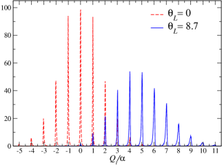
Figure 1: Distribution of the ratio $Q_{t}/\alpha$, for $\beta=6.2$ configurations at $\theta_{L}=0$ and $\theta_{L}=8.7$ ($\theta_{i}\approx 1.5$).
a

The nonperturbative formulation of the above theory on the lattice requires a discretization of the action, $S_{L}-\theta_{L}Q_{L}$; for $S_{L}$ we use the plaquette gluon action, while for $Q_{L}$ we employ the “twisted double plaquette” operator $q_{L}$ ($Q_{L}=\sum_{x}q_{L}(x)$). Notice that this is not the only possible choice for $q_{L}$ ; the only requirement is that it have the correct continuum limit when $a\to 0$ ($a$: lattice spacing). In the continuum limit $q_{L}(x)$, being a local operator, behaves as

$$q_{L}(x)\longrightarrow a^{4}Z_{q}\,q(x)+O(a^{6}),$$ (7)

where $Z_{q}$ is a finite function of the bare coupling $g_{0}$, going to one in the limit $\beta\equiv 2N/g_{0}^{2}\rightarrow\infty$. Thus, we have the correspondence: $\theta_{i}=Z_{q}\,\theta_{L},$ apart from $O(a^{2})$ corrections. The renormalization $Z_{q}$ may be evaluated by MC simulation at $\theta=0$, computing

$$Z_{q}=\langle QQ_{L}\rangle_{\theta=0}/\langle Q^{2}\rangle_{\theta=0}\,,$$ (8)

where $Q$ is an estimator such as those obtained by the overlap method or the cooling method, which are not affected by renormalizations, nor by nonphysical contact terms. Thus, the ratios

$$\langle Q\rangle_{\theta_{i}}/\langle Q^{2}\rangle_{\theta=0}=\theta_{i}-2b_{2}\theta_{i}^{3}+3b_{4}\theta_{i}^{5}+...,\qquad\langle Q^{2}\rangle^{c}_{\theta_{i}}/\langle Q^{2}\rangle_{\theta=0}=1-6b_{2}\theta_{i}^{2}+15b_{4}\theta_{i}^{4}+...,$$ (9)

are expected to have a well defined continuum limit as functions of $\theta_{i}$ .

We have carried out MC simulations of the 4D SU(3) lattice gauge theory, at $\beta=5.9,\,6,\,6.2$, for lattice sizes $L=16,\,16,\,20$, respectively; the simulations are carried out both at $\theta_{L}=0$ and $\theta_{L}\neq 0$, within the region $|\theta_{i}|\mathrel{\hbox to0.0pt{\lower 3.0pt\hbox{$\mathchar 536\relax$}\hss}\raise 2.0pt\hbox{$\mathchar 316\relax$}}\pi$. Since our numerical study requires high-statistics MC simulations, we choose the cooling method as estimator of the topological charge $Q$. The topological charge has been measured on cooled configurations (by locally minimizing the lattice action), using the twisted double plaquette operator. As is well known, this procedure leads to values $Q_{t}\simeq k\alpha$, where $k$ is an integer and $\alpha\mathrel{\hbox to0.0pt{\lower 3.0pt\hbox{$\mathchar 536\relax$}\hss}\raise 2.0pt\hbox{$\mathchar 316\relax$}}1$. Once we determine $\alpha$, we assign to $Q$ the integer closest to $Q_{t}/\alpha$. This cooling method for estimating $Q$, though less rigorous than the significantly more expensive overlap method, produces results in good agreement with it.

Fig. 1 shows the distributions of the ratio $Q_{t}/\alpha$ of $\beta=6.2$ cooled configurations at $\theta_{L}=0$ and $\theta_{L}=8.7$ ($\theta_{i}=Z_{q}\theta_{L}\approx 1.5$). We note that these distributions cluster around integer values, also for rather large values of $Q_{t}/\alpha$, both for $\theta_{L}=0$ and $\theta_{L}=8.7$.

MC simulations at $\theta=0$ were performed at $\beta=5.9,\,6.0,\,6.2$. Over 40 million sweeps per value of $\beta$ were produced. The results for $\chi$, $b_{2}$, $b_{4}$ and $Z_{q}$ are reported in Ref. [2]. Providing our improved estimate of high-order coefficients, such as $b_{4}$, turned out to be very hard in $\theta=0$ MC simulations, requiring huge statistics. The results for $b_{4}$ are consistent with zero, suggesting the bound $|b_{4}|\mathrel{\hbox to0.0pt{\lower 3.0pt\hbox{$\mathchar 536\relax$}\hss}\raise 2.0pt\hbox{$\mathchar 316\relax$}}0.005$, which is improved in $\theta\neq 0$ runs. Our estimates of $Z_{q}$ (e.g. $Z_{q}(\beta=6.0)=0.135(1)$ ) reduce the uncertainty on $Z_{q}$ as produced by other methods.

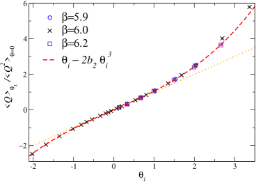
Figure 2: $\langle Q\rangle_{\theta_{L}}/\langle Q^{2}\rangle_{\theta=0}$ vs $\theta_{i}=Z_{q}\theta_{L}$.

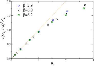
Figure 3: $\langle Q\rangle_{\theta_{L}}/\langle Q^{2}\rangle^{c}_{\theta_{L}}$ vs $\theta_{i}=Z_{q}\theta_{L}$.

MC simulations at $\theta_{L}\neq 0$ are slower by approximately a factor of three, due to the complexity of the action. In $\theta_{L}\neq 0$ runs, $\sim 3$ million sweeps were produced for each value of $\beta$ and $\theta_{L}$. Figs. 3 and 3 show results for the ratios $\langle Q\rangle_{\theta_{L}}/\langle Q^{2}\rangle_{\theta=0}$ and $\langle Q\rangle_{\theta_{L}}/\langle Q^{2}\rangle^{c}_{\theta_{L}}$, versus $\theta_{i}=Z_{q}\theta_{L}$ (cf. Eq. (9) ). The MC data at different $\beta$ values follow the same curve, providing evidence of scaling. Scaling corrections, expected to be $O(a^{2})$, are quite small, and tend to increase with increasing $\theta_{i}$. This good scaling behavior corroborates the existence of a nontrivial continuum limit for any value of $\theta_{i}$. Fitting our data to Eqs. (5,6,9) improves significantly the $\theta=0$ results. In particular, a much smaller bound on $b_{4}$ is obtained: $|b_{4}|<0.001$ ; also, we find: $b_{2}=-0.026(3)$, which is clearly more precise than the estimate obtained from $\theta=0$ runs only: $b_{2}=-0.029(7)$.

Besides allowing more precise determinations of the $\theta$ expansion coefficients of the ground-state energy and other observables, using imaginary $\theta$ values might turn out useful in overcoming the dramatic critical slowing down of topological modes, by performing parallel tempering simulations with a set of $\theta$ values including $\theta{=}0$; this is an exact MC algorithm for the model.

References

References

[1] E. Vicari and H. Panagopoulos,
dependence of SU(N) gauge theories in the presence of a topological
term, Phys. Rep. 470 (2009) 93 [arXiv:0803.1593 hep-th].
[2] H. Panagopoulos and E. Vicari, The 4D SU(3) gauge
theory with an imaginary term, JHEP 11 (2011) 119 [arXiv:1109.6815].