Scaling Algorithms for Approximate
and Exact Maximum Weight Matching

Abstract

The maximum cardinality and maximum weight matching problems can be solved in time $\tilde{O}(m\sqrt{n})$, a bound that has resisted improvement despite decades of research. (Here $m$ and $n$ are the number of edges and vertices.) In this article we demonstrate that this “$m\sqrt{n}$ barrier” is extremely fragile, in the following sense. For any $\epsilon>0$, we give an algorithm that computes a $(1-\epsilon)$-approximate maximum weight matching in $O(m\epsilon^{-1}\log\epsilon^{-1})$ time, that is, optimal linear time for any fixed $\epsilon$. Our algorithm is dramatically simpler than the best exact maximum weight matching algorithms on general graphs and should be appealing in all applications that can tolerate a negligible relative error.

Our second contribution is a new exact maximum weight matching algorithm for integer-weighted bipartite graphs that runs in time $O(m\sqrt{n}\log N)$. This improves on the $O(Nm\sqrt{n})$-time and $O(m\sqrt{n}\log(nN))$-time algorithms known since the mid 1980s, for $1\ll\log N\ll\log n$. Here $N$ is the maximum integer edge weight.

1 Introduction

Graph matching is one of the most well studied problems in combinatorial optimization. The original motivations of the problem were minimizing transportation costs [62, 71] and optimally assigning personnel to job positions [29, 107]. Over the years matching algorithms have found applications in scheduling, approximation algorithms, network switching, and as key subroutines in other optimization algorithms, for example, undirected shortest paths [82], planar max cut [93, 55], Chinese postman tours [32, 81], and metric traveling salesman [15]. In most practical applications it is not critical that the algorithm produce an exactly optimum solution. In this article we explore the extent to which this freedom—not demanding exact solutions—allows us to design simpler and more efficient algorithms.

In order to discuss prior work with precision we must introduce some notation and terminology. The input is a weighted graph $G=(V,E,w)$ where $n=|V|$ and $m=|E|$ are the number of vertices and edges and $w$ is the edge weight function. If $w$ assigns integer (rather than real) weights, let $N$ be the largest magnitude of a weight. An unweighted graph is one for which $w(e)=1$ for all $e\in E$. A matching is a set of vertex-disjoint edges and a perfect matching is one in which all vertices are matched. The weight of a matching is the sum of its edge weights. We use mwm (and mwpm) to denote the problem of finding a maximum weight (perfect) matching, as well as the matching itself. We use mcm and mcpm for the cardinality (unweighted) versions of these problems. The mwpm problem on bipartite graphs is often called the assignment problem.

Table 1: Cardinality Matching

Year	Authors	Time Bound & Notes
	folklore/trivial	$mn$ bipartite
1965	Edmonds	poly$(n)$
1965	Witzgall & Zahn
1969	Balinski
1974	Kameda & Munro
1976	Gabow	$mn$ or $mn\alpha(m,n)$ or $n^{3}$
1976	Lawler
1976	Karzanov
1971	Hopcroft & Karp
1973	Dinic & Karzanov	$m\sqrt{n}$ bipartite
1980	Micali & Vazirani
1991	Gabow & Tarjan	$m\sqrt{n}$
1981	Ibarra & Moran	$n^{\omega}$           cardinality only,randomized,bipartite
		$n^{\omega}$ cardinality only,randomized
1989	Rabin & Vazirani	$n^{\omega+1}$ randomized
1991	Alt, Blum, Mehlhorn & Paul	$n\sqrt{nm/\log n}$ bipartite
1991	Feder & Motwani
1997	Goldberg & Kennedy	$m\sqrt{n}/\kappa$ bipartite, $\kappa=\frac{\log n}{\log(n^{2}/m)}$
1996	Cheriyan & Mehlhorn	$n^{2}+n^{5/2}/w$ bipartite, $w=$ machine word size
2004	Goldberg & Karzanov	$m\sqrt{n}/\kappa$
2004	Mucha & Sankowski
2006	Harvey	$n^{\omega}$ randomized
Note: Here $\omega<2.376$ is the exponent of $n\times n$ matrix multiplication.

The mwpm and mwm problems are reducible to each other. Given an instance $G$ of mwm, let $G^{\prime}$ consist of two copies of $G$ with zero-weight edges connecting copies of the same vertex. Clearly a mwpm in $G^{\prime}$ corresponds to a pair of mwms in $G$. In the reverse direction, if $G$ is an instance of mwpm with weight function $w$, find the mwm of $G$ using the weight function $w^{\prime}(e)=w(e)+nN$. Maximum weight matchings with respect to $w^{\prime}$ necessarily have maximum cardinality. Call a matching $\delta$-approximate, where $\delta\in[0,1]$, if its weight is at least a factor $\delta$ of the optimum matching. Let $\delta$-mwm (and $\delta$-mcm) be the problem of finding $\delta$-approximate maximum weight (cardinality) matching, as well as the matching itself.

Tables 1, 2, and 3 give an at-a-glance history of exact matching algorithms. Algorithms are dated according to their initial publication, and are included either because they establish a new time bound, or employ a noteworthy technique, or are of historical interest. Table 4 gives a history of approximate mcm and mwm algorithms.

1.1 Algorithms for Bipartite Graphs

The mwm problem is expressible as the following integer linear program, where $x$ represents the incidence vector of the matching.

maximize $$\sum_{e\in E}w(e)x(e)$$

subject to $$0\leq x(e)\leq 1 \forall e\in E$$ (1)

$$\sum_{e=(u,u^{\prime})\in E}x(e)\leq 1 \forall u\in V$$

$$x(e) \forall e\in E$$ is an integer (2)

It is well known that in bipartite graphs the integrality requirement (2) is redundant, that is, the basic feasible solutions of the LP (1) are nonetheless integral. See [10, 18]. The dual of (1) is

minimize $$\sum_{u\in V}y(u)$$

subject to $$y(e)\geq w(e) \forall e\in E$$ (3)

$$y(u)\geq 0 \forall u\in V$$

where, by definition, $$y(u,v)\stackrel{{\scriptstyle\rm def}}{{=}}y(u)+y(v)$$

Table 2: Weighted Matching: Bipartite Graphs

Year	Authors	Time Bound & Notes
1946	Easterfield	$2^{n}\mathrm{poly}(n)$
1953	von Neumann
1955	Kuhn
1955	Gleyzal	$\mathrm{poly}(n)$
1957	Munkres
1964	Balinski & Gomory
1969	Dinic & Kronrod	$n^{3}$
1970	Edmonds & Karp	$\mathrm{SP}^{+}=$ time for one SSSP computation on
1971	Tomizawa	$n\cdot\mathrm{SP}^{+}$ a non-negatively weighted graph
1975	Johnson	$mn\log_{d}n$ $d=2+m/n$
		$mn^{3/4}\log N$ integer weights
1983	Gabow	$Nm\sqrt{n}$ mwm only, integer weights
1984	Fredman & Tarjan	$mn+n^{2}\log n$
1988	Gabow & Tarjan
1992	Orlin & Ahuja	$m\sqrt{n}\log(nN)$ integer weights
1997	Goldberg & Kennedy
1996	Cheriyan & Mehlhorn	$n^{5/2}\log(nN)(\frac{\log\log n}{\log n})^{1/4}$ integer weights
		$Nm\sqrt{n}/\kappa$ mwm only, integer weights
1999	Kao, Lam, Sung & Ting	$N(n^{2}+n^{5/2}/w)$ mwm only, integer weights
2004	Mucha & Sankowski	$Nn^{\omega}$               mwm only, randomized, integer weights
2006	Sankowski	$Nn^{\omega}$ randomized, integer weights
		$m\sqrt{n}\log N$ mwm only, integer weights
new		$m\sqrt{n}\log(nN)$ integer weights
Note: $N$ is the maximum integer edge weight, $w$ is the machine word size, and $\kappa=\log n/\log(n^{2}/m)$. The time bounds of Johnson [70] and Fredman and Tarjan [36] reflect faster priority queues. The time bound of Mucha and Sankowski [88] follows from Kao et al.’s [72] reduction.

(In the mwpm problem $\sum_{e=(u,u^{\prime})}x(e)=1$ holds with equality in the primal and $y(u)$ is unconstrained in the dual.) Kuhn’s [76, 78] publication of the Hungarian method stimulated research on this problem from an algorithmic perspective, but it was not without precedent. Kuhn noted that the algorithm was latent in the work of Hungarian mathematicians König and Egerváry. However, the history goes back even further. A recently rediscovered article of Jacobi from 1865 describes a variant of the Hungarian algorithm; see [90]. Although Kuhn’s algorithm self-evidently runs in polynomial time, this mark of efficiency was noted later: Munkres [89] showed that $O(n^{4})$ time is sufficient.

Kuhn’s Hungarian algorithm is sometimes described as a dual (rather than primal) algorithm, due to the fact that it maintains feasibility of the dual (3) and progressively improves the primal objective (1) by finding augmenting paths. Gleyzal [50] (see also [8]) gave a primal algorithm for the assignment problem in which the primal is feasible (the current matching is perfect) and the dual objective is progressively improved via weight-augmenting cycles.

The search for faster assignment algorithms began in earnest in the 1960s. Dinic and Kronrod [24] gave an $O(n^{3})$-time algorithm and Edmonds and Karp [33] and Tomizawa [111] observed that assignment is reducible to $n$ single-source shortest path computations on a non-negatively weighted directed graph. Using Fibonacci heaps, $n$ executions of Dijkstra’s [21] shortest path algorithm take $O(mn+n^{2}\log n)$ time. On integer weighted graphs this algorithm can be implemented slightly faster, in $O(mn+n^{2}\log\log n)$ time [57, 109] or $O(mn)$ time (randomized) [4, 110], independent of the maximum edge weight. Gabow and Tarjan [46], improving an earlier algorithm of Gabow [41], gave a scaling algorithm for the assignment problem running in $O(m\sqrt{n}\log(nN))$ time, which is just a $\log(nN)$ factor slower than the fastest mcm algorithm [65]. For reasonably sparse graphs Gabow and Tarjan’s [46] assignment algorithm remains unimproved. However, faster algorithms have been developed when $N$ is small or the graph is dense [14, 72, 103]. Of particular interest is Sankowski’s algorithm [103], which solves mwpm in $O(Nn^{\omega})$ time, where $\omega$ is the exponent of square matrix multiplication.

1.2 Algorithms for General Graphs

Whereas the basic solutions to (1,3) are integral on bipartite graphs, the same is not true for general graphs. For example, if the graph is a unit-weighted cycle with length $2k+1$ the mwm has weight $k$ but (1) achieves its maximum of $k+1/2$ by setting $x(e)=1/2$ for all $e\in E$. Let $\mathcal{V}_{\operatorname{odd}}$ be the set of all odd-size subsets of $V$. Clearly every feasible solution to the integer linear program (1,2) also satisfies the following odd-set constraints.

$$\sum_{e\in E(B)}x(e)\leq(|B|-1)/2 \forall B\in\mathcal{V}_{\operatorname{odd}}$$ (4)

Table 3: Weighted Matching: General Graphs

Year	Authors	Time Bound & Notes
1965	Edmonds	$\mathrm{poly}(n)$
1974	Gabow
1976	Lawler	$n^{3}$
1976	Karzanov	$n^{3}+mn\log n$
1978	Cunningham & Marsh	$\mathrm{poly}(n)$
1982	Galil, Micali & Gabow	$mn\log n$
		$mn^{3/4}\log N$ integer weights
1985	Gabow	$Nm\sqrt{n}$ mwm only, integer weights
1989	Gabow, Galil & Spencer	$mn\log\log\log_{d}n+n^{2}\log n$ $d=2+m/n$
1990	Gabow	$mn+n^{2}\log n$
1991	Gabow & Tarjan	$m\sqrt{n\log n}\log(nN)$ integer weights
2006	Sankowski	$Nn^{\omega}$ weight only, integer weights
		$Nm\sqrt{n}/\kappa$ mwm only, integer weights
2012	Huang & Kavitha	$Nn^{\omega}$      mwm only, randomized, integer weights
Note: $N$ is the maximum integer edge weight, $\omega$ is the exponent of $n\times n$ matrix multiplication, and $\kappa=\log n/\log(n^{2}/m)$.

Edmonds [30, 31] proved that if we replace the integrality constraints (2) with (4), the basic solutions to the resulting LP are integral. Edmonds’ algorithm mimics the structure of the Hungarian algorithm but the search for augmenting paths is complicated by the presence of odd-length alternating cycles and the fact that matched edges must be searched in both directions. Edmonds’ solution is to contract blossoms as they are encountered. A blossom is defined inductively as an odd-length cycle alternating between matched and unmatched edges, whose components are either single vertices or blossoms in their own right. Blossoms are discussed in detail in Section 2.1.

The fastest implementation of Edmonds’ algorithm, due to Gabow [42], runs in $O(mn+n^{2}\log n)$ time, which matches the running time of the best bipartite mwpm algorithm [36]. Gabow and Tarjan [47] extended their scaling algorithm for mwpm to general graphs, achieving a running time of $O(m\sqrt{n\log n}\log(nN))$, which is the fastest known algorithm for integer-weighted graphs and nearly matches the $O(m\sqrt{n})$ time bound of the best mcm algorithms [86, 113]. As in the bipartite case, faster algorithms for mwm and mwpm are known when the graph is dense or $N$ is small. Sankowski [103] noted that the weight of the mwpm could be computed in $O(Nn^{\omega})$ time; however, it remains an open problem to adapt the cardinality matching algorithms of [88, 60] to weighted graphs. Huang and Kavitha [66], generalizing [72], proved that mwm is reducible to $N$ mcm computations, which, by virtue of [53, 88, 60], implies a new bound of $O(N\cdot\min\{n^{\omega},m\sqrt{n}\log(n^{2}/m)/\log n\})$.

Table 4: Approximate Maximum Cardinality/Weight Matching

Year	Authors	Approx. Problem	Time Bound & Notes
1971	Hopcroft & Karp
1973	Dinic & Karzanov	$(1-\epsilon)$-mcm	$m\epsilon^{-1}$ bipartite
1980	Micali & Vazirani
1991	Gabow & Tarjan	$(1-\epsilon)$-mcm	$m\epsilon^{-1}$
	folklore/trivial	$\frac{1}{2}$-mwm	$m\log n$
1988	Gabow & Tarjan	$(1-\epsilon)$-mwm	$m\sqrt{n}\log(n/\epsilon)$ bipartite
1991	Gabow & Tarjan	$(1-\epsilon)$-mwm	$m\sqrt{n\log n}\log(n/\epsilon)$
1999	Preis
2003	Drake & Hougardy	$\frac{1}{2}$-mwm	$m$
2003	Drake & Hougardy	$(\frac{2}{3}-\epsilon)$-mwm	$m\epsilon^{-1}$
2004	Pettie & Sanders	$(\frac{2}{3}-\epsilon)$-mwm	$m\log\epsilon^{-1}$
2010	Duan & Pettie
2010	Hanke & Hougardy	$(\frac{3}{4}-\epsilon)$-mwm	$m\log n\log\epsilon^{-1}$
2010	Hanke & Hougardy	$(\frac{4}{5}-\epsilon)$-mwm	$m\log^{2}n\log\epsilon^{-1}$
			$m\epsilon^{-1}\log\epsilon^{-1}$     arbitrary weights
new		$(1-\epsilon)$-mwm	$m\epsilon^{-1}\log N$ integer weights
Note: $N$ is the maximum integer edge weight and $\epsilon>0$ is arbitrary.

1.3 Approximating Weighted Matching

The approximate mwm problem is remarkable in that it has been studied for decades, has practical applications, and yet, as late as 1999, essentially nothing better than the greedy algorithm was known. Moreover, the $(1-\epsilon)$-mcm problem had been solved satisfactorily in the early 1970s. Although not stated as such, the $O(m\sqrt{n})$-time exact mcm algorithms [65, 23, 74, 86] are actually $(1-\epsilon)$-mcm algorithms running in $O(m\epsilon^{-1})$ time. These algorithms are based on three observations (i) a maximal set of shortest augmenting paths can be found in linear time, (ii) augmenting along such a set increases the length of the shortest augmenting path, and (iii) that after $k$ rounds of such augmentations the resulting matching is a $(1-\frac{1}{k+1})$-mcm.

Preis [97] gave a linear time $\frac{1}{2}$-mwm algorithm, which improves on the greedy algorithm’s $O(m\log n)$ running time but not its approximation guarantee. Drake and Hougardy [114] presented the first linear time algorithm with an approximation guarantee greater than $1/2$. Specifically, they gave a $(\frac{2}{3}-\epsilon)$-mwm algorithm running in $O(m\epsilon^{-1})$ time, for any $\epsilon>0$. The dependence on $\epsilon$ was later improved by Pettie and Sanders [96]. These algorithms are based on a weighted version of Hopcroft and Karp’s [65] argument, namely that any matching whose weight-augmenting paths and cycles have at least $k$ unmatched edges is necessarily a $(1-\frac{1}{k})$-mwm. Algorithms are presented in [27, 58, 59] with different time/approximation tradeoffs: a $(\frac{3}{4}-\epsilon)$-mwm algorithm running in time $O(m\log n\log\epsilon^{-1})$ and a $(\frac{4}{5}-\epsilon)$-mwm algorithm running in $O(m\log^{2}n\log\epsilon^{-1})$ time.

1.4 New Results

We present the first $(1-\epsilon)$-mwm algorithm that significantly improves on the $\tilde{O}(m\sqrt{n})$ running times of [46, 47]. Our algorithm runs in $O(m\epsilon^{-1}\log\epsilon^{-1})$ time on general graphs and $O(\min\{m\epsilon^{-1}\log\epsilon^{-1},m\epsilon^{-1}\log N\})$ time on integer-weighted general graphs. This is optimal for any fixed $\epsilon$ and near-optimal as a function of $\epsilon$, given the state-of-the-art in mcm algorithms. Moreover, our algorithm is as simple as one could reasonably hope for. Its search for augmenting paths uses depth first search [47, §8] rather than the double depth first search of [86]. It uses no priority queues, split-findmin structures [40], or the blossom “shells” that arise from Gabow and Tarjan’s [47] scaling technique.

Our second result is a new algorithm for exact mwm on bipartite graphs running in $O(m\sqrt{n}\log N)$ time, which improves on [41, 46] for $1\ll\log N\ll\log n$. According to the mwpm$\rightarrow$mwm reduction, this also yields a new $O(m\sqrt{n}\log(nN))$ mwpm algorithm, matching the performance of [46]. However, our algorithm can be used to solve mwpm directly, in $\log(\sqrt{n}N)$ scales rather than $\log(nN)$, which might be practically significant. In terms of technique, our algorithm is a synthesis of the dual (Hungarian-type) approach of Gabow and Tarjan [46] and the primal approach of Balinski and Gomory [8], among others. The $\sqrt{n}$ factor in our running time arises not from the standard blocking flow-type argument [74, 65] but Dilworth’s lemma [22], which ensures that every partial order on $n$ elements contains a chain or anti-chain with size $\sqrt{n}$. Dilworth’s lemma has also been used in Goldberg’s [52] single-source shortest path algorithm.

1.5 Remarks on Approximate Weighted Matching and Its Applications

Our focus is on algorithms that accept arbitrary input graphs and that give provably good worst-case approximations. These twin objectives are self-evidently attractive, yet nearly all work (prior to Preis [97]) on approximate weighted matching focused on specialized cases or weaker approximation guarantees. Early work on the problem usually considered complete bipartite graphs, and confirmed the efficiency of heuristics either experimentally or analytically with respect to inputs over some natural distribution [11, 107, 87, 79, 80, 5]. See Avis [6] for a more detailed discussion of heuristics.

Most work in the area considers graphs defined by metrics, often Euclidean metrics. Reingold and Tarjan [100] proved that the greedy algorithm for metric mwpm has an approximation ratio of $\approx n^{\log\frac{3}{2}}>n^{0.58}$. Goemans and Williamson [51] gave a 2-approximation for metric mwpm that can be implemented in $O(n^{2})$ time [44], or $O(m\log^{2}n)$ time [16] in metrics defined by $m$-edge graphs. The Euclidean mwpm comes in two flavors: the monochromatic version is given $2n$ points and the bichromatic version is given $2n$ points, $n$ of which are colored blue, the rest red, where the matching cannot include monochromatic edges. Varadarajan and Agarwal [112] gave $(1+\epsilon)$-mwpm algorithms for the mono- and bichromatic variants running in time $O(n\mathrm{poly}(\epsilon^{-1}\log n))$ and $O(n^{3/2}\mathrm{poly}(\epsilon^{-1}\log n))$, respectively. Other time-approximation tradeoffs for the bichromatic variant are possible [1, 13], including an $O(n\mathrm{poly}(\log n))$ time algorithm for $O(1)$-approximating the weight of the mwpm [68]. Some work considers the even more specialized case of Euclidean matching in the unit square, which allows for algorithms that guarantee absolute upper bounds on the weight of the matching; see [69, 99, 6] and the references therein.

There are several applications of mwm (on general or bipartite graphs) in which one would gladly sacrifice matching quality for speed. In input-queued switches packets are routed across a switch fabric from input to output ports. In each cycle one partial permutation can be realized. Existing algorithms for choosing these matchings, such as iSLIP [84] and PIM [3], guarantee $\frac{1}{2}$-mcms and it has been shown [85, 49] that (approximate) mwms have good throughput guarantees, where edge weights are based on queue-length. See also [83, 106, 105]. Approximate mwm algorithms are a component in several multilevel graph clustering libraries. (PARTY, for example, builds a hierarchical clustering by iteratively finding and contracting approximate mwms; see [98].) Approximate mwm algorithms are used as a heuristic preprocessing step in several sparse linear system solvers [91, 28, 104, 56]. The goal is to permute the rows/columns to maximize the weight on or near the main diagonal.

1.6 Organization

Section 2 introduces some notation, states well known properties of augmenting paths and blossoms, and reviews Edmonds’ optimality conditions for weighted matching. In Section 3 we present our $(1-\epsilon)$-mwm algorithm and in Section 4 we present exact algorithms for bipartite mwm and mwpm.

2 Preliminaries

We use $E(H)$ and $V(H)$ to refer to the edge and vertex sets of $H$ or the graph induced by $H$, that is, $V(E^{\prime})$ is the set of endpoints of $E^{\prime}\subseteq E$ and $E(V^{\prime})$ is the edge set of the graph induced by $V^{\prime}\subseteq V$. A matching $M$ is a set of vertex-disjoint edges. Vertices not incident to an $M$ edge are free. An alternating path (or cycle) is one whose edges alternate between $M$ and $E\backslash M$. An alternating path $P$ is augmenting if $P$ begins and ends at free vertices, that is, $M\oplus P\stackrel{{\scriptstyle\rm def}}{{=}}(M\backslash P)\cup(P\backslash M)$ is a matching with cardinality $|M\oplus P|=|M|+1$.

When we seek $(1-\epsilon)$ approximate solutions, we can afford to scale and round edge weights to small integers. To see this, observe that the weight of the mwm is at least $w_{\max}=\max\{w(e)\;|\;e\in E(G)\}$. It suffices to find a $(1-\epsilon/2)$-mwm $M$ with respect to the weight function $\tilde{w}(e)=\lfloor w(e)/\gamma\rfloor$ where $\gamma=\epsilon\cdot w_{\max}/n$. Note that $w(e)-\gamma<\gamma\cdot\tilde{w}(e)\leq w(e)$ for any $e$. It follows from the definitions that:

$$w(M) \geq\gamma\cdot\tilde{w}(M) \tilde{w}$$ Defn. of

$$\geq\gamma\cdot(1-\epsilon/2)\tilde{w}(M^{*}) M M^{*}$$ Defn. of , is the mwm

$$>(1-\epsilon/2)(w(M^{*})-\gamma n/2) \tilde{w} |M^{*}|\leq n/2$$ Defn. of ,

$$=(1-\epsilon/2)(w(M^{*})-\epsilon\cdot w_{\max}/2) \gamma$$ Defn. of

$$>(1-\epsilon)w(M^{*}) w(M^{*})\geq w_{\max}$$ Since

Since it is better to use an exact mwm algorithm when $\epsilon<1/n$ [42, 47], we assume, henceforth, that $w\>:\>E\rightarrow\{1,2,\ldots,N\}$, where $N\leq n^{2}$ is the maximum integer edge weight. For notational convenience we also assume that $N$ is a power of 2.

2.1 Blossoms and the LP Formulation of MWM

The dual LP of (1,4) is

minimize $$\sum_{u\in V(G)}y(u)+\sum_{B\in\mathcal{V}_{\operatorname{odd}}}\frac{|B|-1}{2}\cdot z(B)$$

subject to $$yz(e)\geq w(e) \forall e\in E(G)$$

$$y(u)\geq 0,z(B)\geq 0 \forall u\in V(G),\forall B\in\mathcal{V}_{\operatorname{odd}}\rule[-8.53581pt]{0.0pt}{8.53581pt}\rule{0.0pt}{0.0pt}$$

where, by definition, $$yz(u,v)\stackrel{{\scriptstyle\rm def}}{{=}}y(u)+y(v)+\sum_{\begin{subarray}{c}B\in\mathcal{V}_{\operatorname{odd}},\\ (u,v)\in E(B)\end{subarray}}\makebox[0.0pt][l]{$z(B)$}$$

Despite the exponential number of primal constraints and dual $z$-variables, Edmonds demonstrated that an optimum matching could be found in polynomial time without maintaining information ($z$-values) on more than $n/2$ elements of $\mathcal{V}_{\operatorname{odd}}$ at any given time. At intermediate stages of Edmonds’ algorithm there is a matching $M$ and a laminar (nested) subset $\Omega\subseteq\mathcal{V}_{\operatorname{odd}}$, where each element of $\Omega$ is identified with a blossom. Blossoms are formed inductively as follows. If $v\in V$ then the set $\{v\}$ is a trivial blossom. An odd length sequence $(A_{0},A_{1},\ldots,A_{\ell})$ forms a nontrivial blossom $B=\bigcup_{i}A_{i}$ if the $\{A_{i}\}$ are blossoms and there is a sequence of edges $e_{0},\ldots,e_{\ell}$ where $e_{i}\in A_{i}\times A_{i+1}$ (modulo $\ell+1$) and $e_{i}\in M$ if and only if $i$ is odd, that is, $A_{0}$ is incident to unmatched edges $e_{0},e_{\ell}$. See Figure 1. The base of blossom $B$ is the base of $A_{0}$; the base of a trivial blossom is its only vertex. The set of blossom edges $E_{B}$ are $\{e_{0},\ldots,e_{\ell}\}$ and those used in the formation of $A_{0},\ldots,A_{\ell}$. The set $E(B)=E\cap(B\times B)$ may, of course, include many non-blossom edges. A short proof by induction shows that $|B|$ is odd and that the base of $B$ is the only unmatched vertex in the subgraph induced by $B$.

Matching algorithms represent a nested set $\Omega$ of active blossoms by rooted trees, where leaves represent vertices and internal nodes represent nontrivial blossoms. A root blossom is one not contained in any other blossom. The children of an internal node representing $B$ are ordered according to the odd cycle that formed $B$, where one child is distinguished as containing the base of $B$. As we will see, it is often possible to treat blossoms as if they were single vertices. Let the contracted graph $G/\Omega$ be obtained by contracting all root blossoms and removing spurious edges. To dissolve a root blossom $B$ means to delete its node in the blossom forest and, in the contracted graph, to replace $B$ with individual vertices $A_{0},\ldots,A_{\ell}$. Lemma 1 summarizes some useful properties of the contracted graph.

Lemma 1.

Let $\Omega$ be a set of blossoms with respect to a matching $M$.

1. If $M$ is a matching in $G$ then $M/\Omega$ is a matching in $G/\Omega$.

2. Every augmenting path $P^{\prime}$ relative to $M/\Omega$ in $G/\Omega$ extends to an augmenting path $P$ relative to $M$ in $G$. (That is, $P$ is obtained from $P^{\prime}$ by substituting for each non-trivial blossom vertex $B$ in $P^{\prime}$ a path through $E_{B}$. See Figure 1(a,b).)

3. If $P$ is an augmenting path and $P/\Omega$ is also an augmenting path relative to $M/\Omega$, then $\Omega$ remains a valid set of blossoms (possibly with different bases) for the augmented matching $M\oplus P$. See Figure 1(a,b).

4. The base $u$ of a blossom $B\in\Omega$ uniquely determines a maximum cardinality matching of $E_{B}$, having size $(|B|-1)/2$. See Figure 1(a,b).

Implementations of Edmonds’ algorithm grow a matching $M$ while maintaining Property 1, which controls the relationship between $M$, $\Omega$ and the dual variables.

Property 1.

(Complementary Slackness Conditions)

1. Nonnegativity: $z(B)\geq 0$ for all $B\in\mathcal{V}_{\operatorname{odd}}$ and $y(u)\geq 0$ for all $u\in V(G)$.

2. Active Blossoms: $\Omega$ contains all $B$ with $z(B)>0$ and all root blossoms $B$ have $z(B)>0$. (Non-root blossoms may have zero $z$-values.)

3. Domination: $yz(e)\geq w(e)$ for all $e\in E$.

4. Tightness: $yz(e)=w(e)$ when $e\in M$ or $e\in E_{B}$ for some $B\in\Omega$.

If the $y$-values of free vertices become zero, it follows from domination and tightness that $M$ is a maximum weight matching, as the following short proof attests. Here $M^{*}$ is any maximum weight matching.

$$w(M) =\sum_{e\in M}w(e)$$

$$=\sum_{e\in M}yz(e)$$ tightness

$$=\sum_{u\in V(G)}y(u)+\sum_{B\in\Omega}\frac{|B|-1}{2}\cdot z(B) \mbox{Note }\sum_{u\in V(G)}y(u)=\sum_{u\in V(M)}y(u)$$

$$\geq\sum_{u\in V(M^{*})}y(u)+\sum_{B\in\Omega}|E(B)\cap M^{*}|\cdot z(B) y,z$$ non-negative

$$=\sum_{e\in M^{*}}yz(e)\;\geq\;w(M^{*})$$ domination

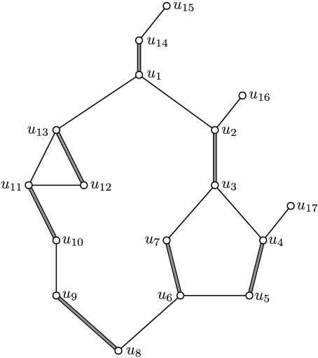
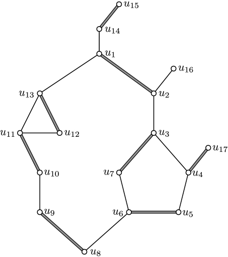
(a)	(b)

Figure 1: Thick edges are matched, thin unmatched. (a) A blossom $B_{1}=(u_{1},u_{2},B_{2},u_{8},u_{9},u_{10},B_{3})$ with base $u_{1}$ containing non-trivial sub-blossoms $B_{2}=(u_{3},u_{4},u_{5},u_{6},u_{7})$ with base $u_{3}$ and $B_{3}=(u_{11},u_{12},u_{13})$ with base $u_{11}$. Vertices $u_{15},u_{16},$ and $u_{17}$ are free. The path $(u_{16},u_{2},u_{3},u_{7},u_{6},u_{5},u_{4},u_{17})$ is an example of an augmenting path that exists in $G$ but not $G/B_{1}$, the graph obtained by contracting $B_{1}$. (b) The situation after augmenting along $(u_{15},u_{14},B_{1},u_{17})$ in $G/B_{1}$, which corresponds to augmenting along $(u_{15},u_{14},u_{1},u_{2},u_{3},u_{7},u_{6},u_{5},u_{4},u_{17})$ in $G$. After augmentation $B_{1}$ and $B_{2}$ have their base at $u_{4}$.

3 A Scaling Algorithm for Approximate mwm

Our algorithm maintains a dynamic relaxation of complementary slackness. In the beginning domination is weak but becomes progressively tighter at each scale whereas tightness is weakened at each scale, though not uniformly. The degree to which a matched edge or blossom edge may violate tightness depends on when it last entered the blossom or matching.

Recall that $N$ is the maximum integer edge weight. The parameter $\epsilon^{\prime}=\Theta(\epsilon)$ will be selected later to guarantee that the final matching is a $(1-\epsilon)$-mwm. Henceforth, assume that $N\geq 1$ and $\epsilon^{\prime}\leq 1/4$ are powers of two. Define $\delta_{0}=\epsilon^{\prime}N$ and $\delta_{i}=\delta_{0}/2^{i}$. At scale $i$ we use the truncated weight function $w_{i}(e)=\delta_{i}\lfloor w(e)/\delta_{i}\rfloor$. Note that $w_{i+1}(e)=w_{i}(e)$ or $w_{i}(e)+\delta_{i+1}$.

Property 2.

(Relaxed Complementary Slackness) There are $L+1$ scales numbered $0,\ldots,L$, where $L=\log N$. Let $i\in[0,L]$ be the current scale.

1. Granularity: $z(B)$ is a nonnegative multiple of $\delta_{i}$, for all $B\in\mathcal{V}_{\operatorname{odd}}$, and $y(u)$ is a nonnegative multiple of $\delta_{i}/2$, for all $u\in V(G)$.

2. Active Blossoms: $\Omega$ contains all $B$ with $z(B)>0$ and all root blossoms $B$ have $z(B)>0$. (Non-root blossoms may have zero $z$-values.)

3. Near Domination: $yz(e)\geq w_{i}(e)-\delta_{i}$ for all $e\in E$.

4. Near Tightness: Call a matched or blossom edge type $j$ if it was last made a matched or blossom edge in scale $j\leq i$. (That is, it entered the set $M\cup\bigcup_{B\in\Omega}E_{B}$ in scale $j$ and has remained in that set, even as $M$ and $\Omega$ evolve as augmenting paths are found and blossoms are formed and dissolved.) If $e$ is such a type $j$ edge then $yz(e)\leq w_{i}(e)+2(\delta_{j}-\delta_{i})$.

5. Free Vertex Duals: The $y$-values of free vertices are equal and strictly less than the $y$-values of matched vertices.

Lemma 2 allows us to measure the quality of a matching $M$, given duals $y$ and $z$ satisfying Property 2.

Lemma 2.

Let $M$ be a matching satisfying Property 2 at scale $i$ and let $M^{*}$ be a maximum weight matching. Let $f$ be the number of free vertices, each having $y$-value $\phi$, and let $\hat{\epsilon}$ be such that $yz(e)-w(e)\leq\hat{\epsilon}\cdot w(e)$ for all $e\in M$. Then $w(M)\geq(1+\hat{\epsilon})^{-1}(w(M^{*})-2\delta_{i}|M^{*}|-f\phi)$. If $i=L$ and $\phi=0$ then $M$ is a $(1-\epsilon^{\prime}-\hat{\epsilon})$-mwm.

Proof.

The claim follows from Property 2.

$$w(M) =\sum_{e\in M}w(e) w(M)$$ defn. of

$$\geq(1+\hat{\epsilon})^{-1}\sum_{e\in M}yz(e) \hat{\epsilon}$$ near tightness, defn. of

$$=(1+\hat{\epsilon})^{-1}\left(\sum_{u\in V(M)}y(u)+\sum_{B\in\Omega}\frac{|B|-1}{2}\cdot z(B)\right) yz$$ defn. of

$$\geq(1+\hat{\epsilon})^{-1}\left(\sum_{u\in V(M^{*})}y(u)+\sum_{B\in\Omega}|E(B)\cap M^{*}|\cdot z(B)-f\phi\right)$$ (5)

$$\geq(1+\hat{\epsilon})^{-1}\left(\sum_{e\in M^{*}}yz(e)-f\phi\right) yz$$ defn. of

$$\geq(1+\hat{\epsilon})^{-1}\left(w_{i}(M^{*})-f\phi-\delta_{i}\cdot|M^{*}|\right)$$ near domination

$$>(1+\hat{\epsilon})^{-1}\left(w(M^{*})-f\phi-2\delta_{i}\cdot|M^{*}|\right) w_{i}$$ defn. of

Inequality (5) follows from several facts, namely, that no matching can contain more than $(|B|-1)/2$ edges in $B$, that $V(M^{*})\backslash V(M)$ contains only free vertices (with respect to $M$), whose $y$-values are $\phi$, and that $y$- and $z$-values are nonnegative. Note that the last inequality is loose by $\delta_{i}|M^{*}|$ if $i=L$ since in that case $w_{L}=w$.

The integrality of edge weights implies that $w(M^{*})\geq|M^{*}|$. If $i=L$ and $\phi=0$ then $\delta_{L}=\epsilon^{\prime}N/2^{L}=\epsilon^{\prime}$ and $w(M)\geq(1+\hat{\epsilon})^{-1}(w(M^{*})-\delta_{L}|M^{*}|)\geq(1+\hat{\epsilon})^{-1}(1-\epsilon^{\prime})w(M^{*})>(1-\epsilon^{\prime}-\hat{\epsilon})w(M^{*})$, that is, $M$ is a $(1-\epsilon^{\prime}-\hat{\epsilon})$-mwm. ∎

While not suggesting an algorithm per se, Lemma 2 tells us which invariants our algorithm must maintain and when it may halt with a $(1-\epsilon)$-mwm. For example, if at the last scale $L$ we have $\delta_{L}\leq\epsilon/2$ and for any type $j$ edge $e\in M$, $\delta_{j}\leq(\epsilon/4)w(e)$ (i.e., $\hat{\epsilon}=\epsilon/2$) then as soon as $y$-values at free vertices reach zero, the current matching must be a $(1-\epsilon)$-mwm.

3.1 The Scaling Algorithm

Initially $M=\emptyset,\Omega=\emptyset$, and $y(u)=N/2-\delta_{0}/2$ for all $u\in V$, which clearly satisfies Property 2 for scale $i=0$, since $yz(e)=2(N/2-\delta_{0}/2)\geq w_{0}(e)-\delta_{0}$. The algorithm, given in Figure 2, consists of scales $0,\ldots,L=\log N$, where the purpose of scale $i$ is to halve the $y$-values of free vertices while maintaining Property 2. In each iteration of scale $i$ the algorithm (1) augments a maximal set of augmenting paths of eligible edges, (2) finds and contracts blossoms of eligible edges, (3) performs dual adjustments on $y$- and $z$-values, and (4) dissolves previously contracted root blossoms if their $z$-values become zero. Each dual adjustment step decrements by $\delta_{i}/2$ the $y$-values of free vertices. Thus, there are roughly $(N/2^{i})/(\delta_{i}/2)=O(\epsilon^{-1})$ iterations per scale, independent of $i$. The efficiency and correctness of the algorithm depend on eligibility being defined properly.

Definition 1.

At scale $i$, an edge $e$ is eligible if at least one of the following hold:

1. $e\in E_{B}$ for some $B\in\Omega$.

2. $e\not\in M$ and $yz(e)=w_{i}(e)-\delta_{i}$.

3. $e\in M$ and $yz(e)-w_{i}(e)$ is a nonnegative integer multiple of $\delta_{i}$.

Let $E_{elig}$ be the set of eligible edges and let $G_{elig}=(V,E_{elig})/\Omega$ be the unweighted graph obtained by discarding ineligible edges and contracting root blossoms.

Criterion (i) for eligibility simply ensures that an augmenting path in $G_{elig}$ extends to an augmenting path of eligible edges in $G$. A key implication of Criteria (ii) and (iii) is that if $P$ is an augmenting path in $G_{elig}$, every edge in $P$ becomes ineligible in $(M/\Omega)\oplus P$. This follows from the fact that unmatched edges must have $yz(e)-w_{i}(e)<0$ whereas matched edges must have $yz(e)-w_{i}(e)\geq 0$. Regarding Criterion (iii), note that Property 2 (granularity and near domination) implies that $yz(e)-w_{i}(e)$ is at least $-\delta_{i}$ and an integer multiple of $\delta_{i}/2$.

Initialization: $\displaystyle M$ $\displaystyle\leftarrow\emptyset$ no matched edges $\displaystyle\Omega$ $\displaystyle\leftarrow\emptyset$ no blossoms $\displaystyle\delta_{0}$ $\displaystyle\leftarrow\epsilon^{\prime}N$ $\epsilon^{\prime}=\Theta(\epsilon)$; w.l.o.g., $\epsilon^{\prime},N$ are powers of 2 $\displaystyle y(u)$ $\displaystyle\leftarrow\frac{N}{2}-\frac{\delta_{0}}{2},\mbox{ for all }u\in V(G)\hskip 199.16928pt$ satisfies Property 2(3) Execute scales $i=0\ldots,L=\log N$ and return the matching $M$. Scale $i$: – Repeat the following steps until $y$-values of free vertices reach $N/2^{i+2}-\delta_{i}/2$, if $i\in[0,L)$, or until they reach zero, if $i=L$.
(1) Augmentation:
Find a maximal set $\Psi$ of augmenting paths in $G_{elig}$ and set $M\leftarrow M\oplus(\bigcup_{P\in\Psi}P)$. Update $G_{elig}$.
(2) Blossom Shrinking:
Let $V_{out}\subseteq V(G_{elig})$ be the vertices (that is, root blossoms) reachable from free vertices by even-length alternating paths; let $\Omega^{\prime}$ be a maximal set of (nested) blossoms on $V_{out}$. (That is, if $(u,v)\in E(G_{elig})\backslash M$ and $u,v\in V_{out}$, then $u$ and $v$ must be in a common blossom.) Let $V_{in}\subseteq V(G_{elig})\backslash V_{out}$ be those non-$V_{out}$-vertices reachable from free vertices by odd-length alternating paths. Set $z(B)\leftarrow 0$ for $B\in\Omega^{\prime}$ and set $\Omega\leftarrow\Omega\cup\Omega^{\prime}$. Update $G_{elig}$.
(3) Dual Adjustment:
Let $\hat{V}_{in},\hat{V}_{out}\subseteq V$ be original vertices represented by vertices in $V_{in}$ and $V_{out}$. The $y$- and $z$-values for some vertices and root blossoms are adjusted: $\displaystyle y(u)$ $\displaystyle\leftarrow y(u)-\delta_{i}/2,\mbox{ for all $u\in\hat{V}_{out}$.}$ $\displaystyle y(u)$ $\displaystyle\leftarrow y(u)+\delta_{i}/2,\mbox{ for all $u\in\hat{V}_{in}$.}$ $\displaystyle z(B)$ $\displaystyle\leftarrow z(B)+\delta_{i},\mbox{ if $B\in\Omega$ is a root blossom with $B\subseteq\hat{V}_{out}$.}$ $\displaystyle z(B)$ $\displaystyle\leftarrow z(B)-\delta_{i},\mbox{ if $B\in\Omega$ is a root blossom with $B\subseteq\hat{V}_{in}$.}\hskip 56.9055pt$ (4) After dual adjustments some root blossoms may have zero $z$-values. Dissolve such blossoms (remove them from $\Omega$) as long as they exist. Note that non-root blossoms are allowed to have zero $z$-values. Update $G_{elig}$ by the new $\Omega$.
– Prepare for the next scale, if $i\in[0,L)$: $\displaystyle\delta_{i+1}$ $\displaystyle\leftarrow\delta_{i}/2$ $\displaystyle y(u)$ $\displaystyle\leftarrow y(u)+\delta_{i+1},\mbox{ for all }u\in V(G).\hskip 142.26378pt$

Figure 2: A $(1-\epsilon)$-approximate mwm algorithm

3.2 Analysis and Correctness

Lemma 5 states that the algorithm maintains Property 2 after each of the $O(\epsilon^{-1})$ Dual Adjustment steps in each scale. Lemma 3 establishes the critical fact that all augmenting paths and paths from free vertices to blossoms are eliminated from $G_{elig}$ before each Dual Adjustment step.

Lemma 3.

After the Augmentation and Blossom Shrinking steps $G_{elig}$ contains no augmenting path, nor is there a path from a free vertex to a blossom.

Proof.

Suppose there is an augmenting path $P$ in $G_{elig}$ after augmenting along paths in $\Psi$. Since $\Psi$ is maximal, $P$ must intersect some $P^{\prime}\in\Psi$ at a vertex $v$. However, after the Augmentation step every edge in $P^{\prime}$ will become ineligible, so the matching edge $(v,v^{\prime})\in M$ is no longer in $G_{elig}$, contradicting the fact that $P$ consists of eligible edges. Since $\Omega^{\prime}$ is maximal there can be no blossom reachable from a free vertex in $G_{elig}$ after the Blossom Shrinking step. ∎

Lemma 4 guarantees that all $y$-values updated in a Dual Adjustment step have the same parity as a multiple of $\delta_{i}/2$. In the proof of Lemma 5 this fact is used to argue that if both endpoints of an edge $e$ have their $y$-values decremented, then $yz(e)$ is a multiple of $\delta_{i}$.

Lemma 4.

Let $R\subseteq V(G_{elig})$ be the set of vertices reachable from free vertices by eligible alternating paths, at any point in scale $i$. Let $\hat{R}\subseteq V(G)$ be the set of original vertices represented by those in $R$. Then the $y$-values of $\hat{R}$-vertices have the same parity, as a multiple of $\delta_{i}/2$.

Proof.

Assume, inductively, that before the Blossom Shrinking step, all vertices in a common blossom have the same parity, as a multiple of $\delta_{i}/2$. Consider an eligible path $P=(B_{0},B_{1},\ldots,B_{k})$ in $G_{elig}$, where the $\{B_{j}\}$ are either vertices or blossoms in $\Omega$ and $B_{0}$ is unmatched in $G_{elig}$. Let $(u_{0},v_{1}),(u_{1},v_{2}),\ldots,(u_{k-1},v_{k})$ be the $G$-edges corresponding to $P$, where $u_{j},v_{j}\in B_{j}$. By the inductive hypothesis, $u_{j}$ and $v_{j}$ have the same parity, and whether $(u_{j},v_{j+1})$ is matched or unmatched, Definition 1 stipulates that $yz(u_{j},v_{j+1})/\delta_{i}$ is an integer, which implies $y(u_{j})$ and $y(v_{j+1})$ have the same parity as a multiple of $\delta_{i}/2$. Thus, the $y$-values of all vertices in $B_{0}\cup\cdots\cup B_{k}$ have the same parity as a free vertex in $B_{0}$, whose $y$-value is equal to every other free vertex, by Property 2(5). Since new blossoms are formed by eligible edges, the inductive hypothesis is preserved after the Blossom Shrinking step. It is also preserved after the Dual Adjustment step since the $y$-values of vertices in a common blossom are incremented or decremented in lockstep. This concludes the induction. ∎

Lemma 5.

The algorithm preserves Property 2.

Proof.

Property 2(5) (free vertex duals) is obviously maintained as only free vertices have their $y$-values decremented in each Dual Adjustment step. Property 2(2) (active blossoms) is also maintained since all the new root blossoms discovered in the Blossom Shrinking step are contained in $V_{out}$ and will have positive $z$-values after adjustment. Furthermore, each root blossom whose $z$-value drops to zero is dissolved, after Dual Adjustment. At the beginning of scale $i$ all $y$- and $z$-values are integer multiples of $\delta_{i}/2$ and $\delta_{i}$, respectively, satisfying Property 2(1) (granularity). This property is clearly maintained in each Dual Adjustment step. If $e\not\in M$ is placed in $M$ during an Augmentation step or placed in $\bigcup_{B\in\Omega}E_{B}$ during a Blossom Shrinking step then $e$ is type $i$ and $yz(e)=w_{i}(e)-\delta_{i}<w_{i}(e)$, which satisfies Property 2(4).

It remains to show that the algorithm maintains Property 2(3,4) (near domination and near tightness). First consider the dual adjustments made at the end of scale $i$ (the last line of pseudocode in Figure 2.) Let $e=(u,v)$ be an arbitrary edge and let $yz$ and $yz^{\prime}$ be the function before and after dual adjustment. It follows that

$$yz^{\prime}(e) =yz(e)+2\delta_{i+1} y(u),y(v) \delta_{i+1}$$ incremented by

$$\geq w_{i}(e)-\delta_{i}+2\delta_{i+1} i$$ near domination at scale

$$\geq w_{i+1}(e)-\delta_{i+1} w_{i}(e)\geq w_{i+1}(e)-\delta_{i+1}$$

That is, Property 2(3) is preserved. If $e\in M\cup\bigcup_{B\in\Omega}E_{B}$ is a type $j$ edge, then at the end of scale $i$ Property 2(4) is also preserved since

$$yz^{\prime}(e)=yz(e)+2\delta_{i+1}\leq w_{i}(e)+2(\delta_{j}-\delta_{i})+2\delta_{i+1}\leq w_{i+1}(e)+2(\delta_{j}-\delta_{i+1})$$

The first inequality follows from Property 2(4) at scale $i$ and the second inequality from the fact that $w_{i}(e)\leq w_{i+1}(e)$ and $\delta_{i}=2\delta_{i+1}$.

Now consider a Dual Adjustment step. If neither $u$ nor $v$ is in $\hat{V}_{in}\cup\hat{V}_{out}$ or if $u,v$ are in the same root blossom in $\Omega$, then $yz(e)$ is unchanged, preserving Property 2. The remaining cases depend on whether $(u,v)$ is in $M$ or not, whether $(u,v)$ is eligible or not, and whether both $u,v\in\hat{V}_{in}\cup\hat{V}_{out}$ or not.

Case 1: $e\not\in M,\,u,v\in\hat{V}_{in}\cup\hat{V}_{out}$

If $e$ is ineligible then $yz(e)>w_{i}(e)-\delta_{i}$. However, by Lemma 4 (parity of $y$-values) we know $(yz(e)-w_{i}(e))/\delta_{i}$ is an integer, so $yz(e)\geq w_{i}(e)$ before adjustment and $yz(e)\geq w_{i}(e)-\delta_{i}$ afterward (which could occur if both $u,v\in\hat{V}_{out}$), thereby preserving Property 2(3). If $e$ is eligible then at least one of $u,v$ is in $\hat{V}_{in}$, otherwise another blossom or augmenting path would have been formed, so $yz(e)$ cannot be reduced, which also preserves Property 2(3).

Case 2: $e\in M,\,u,v\in\hat{V}_{in}\cup\hat{V}_{out}$

Since $u,v\in\hat{V}_{in}\cup\hat{V}_{out}$, Lemma 4 (parity of $y$-values) guarantees that $(yz(e)-w_{i}(e))/\delta_{i}$ is an integer. The only way $e$ can be ineligible is if $yz(e)=w_{i}(e)-\delta_{i}$ and $u,v\in\hat{V}_{in}$, hence $yz(e)=w_{i}(e)$ after dual adjustment, which preserves Property 2(3,4). On the other hand, if $e$ is eligible then $u\in\hat{V}_{in}$ and $v\in\hat{V}_{out}$. It cannot be that $u,v\in\hat{V}_{out}$, otherwise $e$ would have been included in an augmenting path or root blossom. In this case $yz(e)$ is unchanged, preserving Property 2(3,4).

Case 3: $e\not\in M,\,v\not\in\hat{V}_{in}\cup\hat{V}_{out}$

If $e$ is eligible then $u\in\hat{V}_{in}$ and $yz(e)$ will increase. If it is ineligible then $yz(e)\geq w_{i}(e)-\delta_{i}/2$ before adjustment and $yz(e)\geq w_{i}(e)-\delta_{i}$ afterward. In both cases Property 2(3) is preserved.

Case 4: $e\in M,\,v\not\in\hat{V}_{in}\cup\hat{V}_{out}$

It must be that $e$ is ineligible, so $u\in\hat{V}_{in}$ and $yz(e)-w_{i}(e)$ is either negative or an odd multiple of $\delta_{i}/2$. If $e$ is type $j$ then, by Property 2(1,4) (granularity and near tightness), $yz(e)\leq w_{i}(e)+2(\delta_{j}-\delta_{i})-\delta_{i}/2$ before adjustment and $yz(e)\leq w_{i}(e)+2(\delta_{j}-\delta_{i})$ afterward, preserving Property 2(4). ∎

Recall that Lemma 2 stated that the final matching will be a $(1-O(\epsilon))$-mwm if $\delta_{L}=O(\epsilon)$, free vertices have zero $y$-values, and $yz(e)-w(e)=O(\epsilon)\cdot w(e)$. Lemmas 6 and 7 establish these bounds.

Lemma 6.

Let $i\leq L$ be the scale index. Then

1. For $i<L$, all edges eligible at any time in scales 0 through $i$ have weight at least $N/2^{i+1}+\delta_{i}$.

2. For any $i$, if $e\in M$ then $yz(e)\leq(1+4\epsilon^{\prime})w(e)$.

Proof.

We prove the parts separately.

Part 1

The last search for augmenting paths in scale $i$ begins when the $y$-values of free vertices are $N/2^{i+2}$, and strictly less than $y$-values of other vertices, by Property 2(5). An unmatched edge $e=(u,v)$ can only be eligible at this scale if $yz(e)=w_{i}(e)-\delta_{i}\leq w(e)-\delta_{i}$. Hence $w(e)\geq y(u)+y(v)+\delta_{i}\geq N/2^{i+1}+\delta_{i}$.

Part 2

Let $e$ be a type $j$ edge in $M$ during scale $i$. Property 2(4) states that $yz(e)-w_{i}(e)\leq 2(\delta_{j}-\delta_{i})$. Since $w_{i}(e)\leq w(e)$ it also follows that $yz(e)-w(e)\leq 2\delta_{j}-2\delta_{i}<2\delta_{j}=\epsilon^{\prime}N/2^{j-1}$. By part 1, a type $j$ edge must have weight at least $N/2^{j+1}+\delta_{j}$, hence $yz(e)-w(e)<4\epsilon^{\prime}\cdot w(e)$. ∎

Lemma 7.

After scale $L=\log N$, $M$ is a $(1-5\epsilon^{\prime})$-mwm.

Proof.

The final scale ends when free vertices have zero $y$-values. Property 2(3) holds with respect to $\delta_{L}=\delta_{0}/2^{L}=\epsilon^{\prime}N/2^{L}=\epsilon^{\prime}$ and Lemma 6 states that $yz(e)\leq(1+4\epsilon^{\prime})w(e)$. By Lemma 2, $w(M)\geq(1-5\epsilon^{\prime})w(M^{*})$. ∎

Theorem 1.

A $(1-\epsilon)$-mwm can be computed in time $O(m\epsilon^{-1}\log N)$.

Proof.

Each Augmentation and Blossom Shrinking step takes $O(m)$ time using a modified depth-first search [47, §8]. (Finding a maximal set of augmenting paths is significantly simpler, conceptually, than finding a maximal set of minimum-length augmenting paths, as is done in [86, 113].) Each Dual Adjustment step clearly takes linear time, as does the dual adjustment at the end of each scale. Scale $i<L=\log N$ begins with free vertices’ $y$-values at $N/2^{i+1}-\delta_{i}$ and ends with them at $N/2^{i+2}-\delta_{i}$. Since $y$-values are decremented by $\delta_{i}/2$ in each Dual Adjustment step there are exactly $(N/2^{i+2})/(\delta_{i}/2)=N/(2\delta_{0})=\epsilon^{\prime-1}/2$ such steps. The final scale begins with free vertices’ $y$-values at $N/2^{L+1}-\delta_{L}$ and ends with them at zero, so there are fewer than $(N/2^{L+1})/(\delta_{L}/2)=\epsilon^{\prime-1}$ Dual Adjustment steps. Lemma 7 guarantees that the final matching is a $(1-\epsilon)$-mwm for $\epsilon^{\prime}\leq\epsilon/5$. Hence, the total running time is $O(m\epsilon^{-1}\log N)$. ∎

3.3 A Linear Time Algorithm

Our $O(m\epsilon^{-1}\log N)$-time algorithm requires few modifications to run in linear time, independent of $N$. In fact, the algorithm as it appears in Figure 2 requires no modifications at all: we only need to change the definition of eligibility and, in each scale, refrain from scanning edges that cannot possibly be eligible or part of augmenting paths or blossoms. In light of Lemma 6(1) it is helpful to index edges according to the first scale in which they may be eligible.

Definition 2.

Define $\mu_{i}=N/2^{i+1}+\delta_{i}$, for $i<L$, and $\mu_{L}=0$. Define $\operatorname{scale}(e)$ to be the $i$ such that $w(e)\in[\mu_{i},\mu_{i-1})$.

Definition 3 redefines eligibility. The differences with Definition 1 are underlined.

Definition 3.

At scale $i$, an edge $e$ is eligible if at least one of the following hold:

1. $e\in E_{B}$ for some $B\in\Omega$.

2. $e\not\in M$ and $yz(e)=w_{i}(e)-\delta_{i}$.

3. $e\in M$ and $yz(e)-w_{i}(e)$ is a nonnegative intelligent multiple of $\delta_{i}$. Furthermore, $\operatorname{scale}(e)\geq i-\gamma$, where $\gamma\stackrel{{\scriptstyle\rm def}}{{=}}\log\epsilon^{\prime-1}$.

Let $E_{elig}$ be the set of eligible edges and let $G_{elig}=(V,E_{elig})/\Omega$ be the unweighted graph obtained by discarding ineligible edges and contracting root blossoms.

Lemma 8.

Using Definition 3 of eligibility rather than Definition 1, Property 2(1,2,3,5) is maintained and Property 2(4) (near tightness) holds in the following weaker form. Let $e\in M\cup\bigcup_{B\in\Omega}E_{B}$ be a type $j$ edge with $\operatorname{scale}(e)=i$. Then $yz(e)\leq w_{k}(e)+2(\delta_{j}-\delta_{k})$ at any scale $k\in[i,i+\gamma]$ and $yz(e)\leq w_{k}(e)+3\delta_{i}<(1+6\epsilon^{\prime})w(e)$ for $k>i+\gamma$.

Proof.

In scales $i$ through $i+\gamma$ Property 2(4) is maintained as the two definitions of eligibility are the same. At the beginning of scale $t=i+\gamma+1$, $e$ is no longer eligible and the $y$-values of free vertices are $N/2^{t+1}-\delta_{t}/2$. From this moment on, the $y$-values of free vertices are incremented by a total of $\sum_{l\geq t+1}\delta_{l}$ (the dual adjustments following scales $t$ through $L-1$) and decremented a total of $N/2^{t+1}-\delta_{t}/2+\sum_{l\geq t+1}\delta_{l}$ (in the Dual Adjustment steps following searches for augmenting paths and blossoms). Each adjustment to $y$-values by some quantity $\Delta$ may cause $yz(e)$ to increase by $2\Delta$. This clearly occurs in the dual adjustments following each scale as $y(u)$ and $y(v)$ are incremented by $\Delta$. Following a search for blossoms it may be that $u,v\in\hat{V}_{in}$, which would also cause $y(u)$ and $y(v)$ to each be incremented by $\Delta$. Note that $y(u),y(v)$ cannot be decremented in scales $t$ through $L$; if either were in $\hat{V}_{out}$ after a search for blossoms then $e$ would have been eligible, a contradiction. Hence Property 2(3) (near domination) is maintained for $e$. Putting this all together, it follows that at any scale $k\geq t=i+\gamma+1=i+\log\epsilon^{\prime-1}+1$,

$$yz(e) \leq w_{k}(e)+2(\delta_{j}-\delta_{k})+2\cdot\left(N/2^{t+1}-\delta_{t}/2+2\cdot\sum_{l\geq t+1}\delta_{l}\right)$$

$$<w_{k}(e)+2\delta_{i}+2\left(\delta_{i+2}+\mbox{$\frac{3}{2}$}\delta_{t}\right) j\geq i t$$ , defn. of

$$=w_{k}(e)+(2+1/2+3\epsilon^{\prime}/2)\delta_{i} \delta_{t}=\epsilon^{\prime}\delta_{i}/2$$ defn. of

$$<w_{k}(e)+3\delta_{i} \epsilon^{\prime}<1/3$$

$$<(1+6\epsilon^{\prime})w(e) w(e)\geq w_{k}(e)>N/2^{i+1}=(2\epsilon^{\prime})^{-1}\cdot\delta_{i}$$

which proves the claim. Note that the inequality $yz(e)<w_{k}(e)+3\delta_{i}$ also holds in scales $k\in[i,i+\gamma]$. If $e$ is type $j\geq i$ then $yz(e)\leq w_{k}(e)+2(\delta_{j}-\delta_{k})<w_{k}(e)+2\delta_{i}$. This fact will be used in Lemma 9. ∎

The algorithm will deliberately ignore unmatched edges that may still be eligible according to Definition 3. This will be justified on the grounds that such edges must be adjacent to matched ineligible edges, and therefore cannot be contained in an eligible augmenting path. Lemma 9 will be used to argue that scale-$i$ edges can be safely ignored after scale $i+\gamma+2$.

Lemma 9.

Let $e_{1}=(u,v)$ be an edge with $\operatorname{scale}(e_{1})=i$ and let $e_{0}=(u^{\prime},u)$ and $e_{2}=(v,v^{\prime})$ be the $M$-edges incident to $u$ and $v$ at some time after scale $i$. Then at least one of $e_{0}$ and $e_{2}$ exists, say $e_{0}$, and $\operatorname{scale}(e_{0})\leq i+2$.

Proof.

Following the last Dual Adjustment step in scale $i$ the $y$-values of free vertices are $N/2^{i+2}-\delta_{i}/2$. It cannot be that both $u$ and $v$ are free at this time, otherwise $yz(e_{1})=y(u)+y(v)=N/2^{i+1}-\delta_{i}=\mu_{i}-2\delta_{i}<w_{i}(e_{1})-\delta_{i}$, violating Property 2(3) (near domination). Hence, either $u$ or $v$ is matched for the remainder of the computation. If $e_{1}$ is matched the claim is trivial, so, assuming the claim is false, whenever $e_{0},e_{2}$ exist we have $\operatorname{scale}(e_{0}),\operatorname{scale}(e_{2})\geq i+3$. That is, $w(e_{0}),w(e_{2})<\mu_{i+2}=N/2^{i+3}+\delta_{i+2}$.

It cannot be that $e_{1}$ is in a blossom without $e_{0}$ or $e_{2}$ also being in the blossom. For any $l\in\{0,1,2\}$ let $\mathcal{B}_{l}\subseteq\Omega$ be the blossoms containing $e_{l}$ at a given time. The laminarity of blossoms ensures that either $\mathcal{B}_{1}\subseteq\mathcal{B}_{0}$ or $\mathcal{B}_{1}\subseteq\mathcal{B}_{2}$. Suppose it is the former, that is, $e_{0}$ exists and $e_{2}$ may or may not exist. Then, if the current scale is $k\geq i+3$, by Property 2(3) (near domination) $yz(e_{1})=y(u)+y(v)+\sum_{B\in\mathcal{B}_{1}}z(B)\geq w_{k}(e_{1})-\delta_{k}$. By Lemma 8 $y(u)+\sum_{B\in\mathcal{B}_{1}}z(B)<yz(e_{0})\leq w_{k}(e_{0})+3\delta_{i+3}$ and, if $e_{2}$ exists, $y(v)<yz(e_{2})\leq w_{k}(e_{2})+3\delta_{i+3}$. These inequalities follow from the definition of $yz$, the containment $\mathcal{B}_{1}\subseteq\mathcal{B}_{0}$ and the fact that $e_{0}$ and $e_{2}$ can only be at scale $i+3$ or higher. Without loss of generality we can assume $y(u)+\sum_{B\in\mathcal{B}_{1}}z(B)\geq y(v)$. (If $e_{2}$ exists and $y(v)>y(u)+\sum_{B\in\mathcal{B}_{1}}z(B)$ then $e_{2}$ takes the role of $e_{0}$ below.) Putting these inequalities together we have

$$w_{k}(e_{1}) \leq y(u)+y(v)+\sum_{B\in\mathcal{B}_{1}}z(B)+\delta_{k}$$ near domination

$$\leq 2\left(y(u)+\sum_{B\in\mathcal{B}_{1}}z(B)\right)+\delta_{k} y(u)+\sum_{B\in\mathcal{B}_{1}}z(B)\geq y(v)$$

$$\leq 2\left(yz(e_{0})\right)+\delta_{k} \mathcal{B}_{1}\subseteq\mathcal{B}_{0}$$

$$<2(w_{k}(e_{0})+3\delta_{i+3})+\delta_{k}$$ Lemma 8

$$<2w(e_{0})+7\delta_{i+3} k\geq i+3 \epsilon^{\prime}<1/3$$ ,

and therefore

$$w(e_{0}) >\mbox{$\frac{1}{2}$}(w_{k}(e_{1})-\delta_{i}) 7\delta_{i+3}<\delta_{i}$$

$$\geq N/2^{i+2} \operatorname{scale}(e_{1})=i,w_{k}(e_{1})\geq\mu_{i}=N/2^{i+1}+\delta_{i}$$

$$>N/2^{i+3}+\delta_{i+2}=\mu_{i+2}$$

This contradicts the fact that $\operatorname{scale}(e_{0})\geq i+3$, since, by definition, such edges have $w(e_{0})<\mu_{i+2}$. ∎

Theorem 2.

A $(1-\epsilon)$-mwm can be computed in time $O(m\epsilon^{-1}\log\epsilon^{-1})$.

Proof.

We execute the algorithm from Figure 2 where $G_{elig}$ refers to the eligible subgraph as defined in Definition 3. We need to prove several claims: (i) the algorithm does, in fact return a $(1-\epsilon)$-mwm for suitably chosen $\epsilon^{\prime}=\Theta(\epsilon)$, (ii) the number of scales in which an edge could conceivably participate in an augmenting path or blossom is $\log\epsilon^{-1}+O(1)$, and (iii) it is possible in linear time to compute the scales in which each edge must participate. Part (i) follows from Lemmas 2 and 8. Since $yz(e)\leq(1+6\epsilon^{\prime})w(e)$ for any $e\in M$ and $\delta_{L}=\epsilon^{\prime}$, Lemma 2 implies that $M$ is a $(1-\epsilon)$-mwm when $\epsilon^{\prime}\leq\epsilon/7$.

Turning to part (ii), consider an edge $e$ with $\operatorname{scale}(e)=i$. By Lemma 6(1) $e$ can be ignored in scales 0 through $i-1$. If $e=(u,v)\in M$ then, according to Definition 3, $e$ will be ineligible in scales $i+\gamma+1$ through $\log N$. After scale $i+\gamma$ no augmenting path or blossom can contain $e$, so we can commit it to the final matching and remove from consideration all edges incident to $u$ or $v$. Now suppose that $e\not\in M$ at the end of scale $i+\gamma+2$. Lemma 9 states that either $u$ or $v$ is incident to a matched edge $e_{0}$ with $\operatorname{scale}(e_{0})\leq i+2$, which by the argument above, will be committed to the final matching, thereby removing $e$ from further consideration. Thus, to faithfully execute the algorithm we only need to consider $e$ in scales $\operatorname{scale}(e)$ through $\operatorname{scale}(e)+\gamma+2$, that is, $\gamma+3=\log\epsilon^{\prime-1}+3\leq\log\epsilon^{-1}+6$ scales in total.

We have narrowed our problem to that of computing $\operatorname{scale}(e)$ for all $e$. This is tantamount to computing the most significant bit ($\operatorname{MSB}(x)=\lfloor\log_{2}x\rfloor$) in the binary representation of $w(e)$. Once the $\operatorname{MSB}$ is known, $\operatorname{scale}(e)$ can be just one of two possible values. MSBs can be computed in a number of ways using standard instructions. It is trivial to extract $\operatorname{MSB}(x)$ after converting $x$ to floating point representation. Fredman and Willard [37] gave an $O(1)$ time algorithm using unit time multiplication. However, we do not need to rely on floating point conversion or multiplication. In Section 2 we showed that without loss of generality $\log N\leq 2\log n$. Using a negligible $O(n^{\beta})$ space and preprocessing time we can tabulate the answers on $\beta\cdot\log n$-bit integers, where $\beta\leq 1$, then compute MSBs with $2\beta^{-1}=O(1)$ table lookups. ∎

4 Exact Maximum Weight Matching

At a high level our exact mwm algorithm is similar to our $(1-\epsilon)$-mwm algorithm. It consists of $\log N+1$ scales, where, in the $i$th scale, the magnitude of dual adjustments and the violation of domination/tightness is bounded in terms of $\delta_{i}$, which decreases geometrically with $i$. However, beyond this similarity the two algorithms are quite different. Our exact mwm algorithm only works on bipartite graphs; we assume for simplicity that the graph consists of exactly $n$ left vertices and $n$ right vertices.

We redefine $\delta_{0}=2^{\lfloor\log(N/\sqrt{n})\rfloor}$ and let $\delta_{i}=\delta_{0}/2^{i}$ and $w_{i}(e)=\delta_{i}\lfloor w(e)/\delta_{i}\rfloor$ be the granularity and weight function of the $i$th scale, where $i\in[0,L]$ and $L=\lceil\log N\rceil$. The algorithm maintains a matching $M$ and duals $y$ satisfying Property 3. (As the graph is bipartite there is no need for blossoms or their duals $z$.) Whereas Property 2 allows domination to be violated by $\delta_{i}$ but enforces tightness of matched edges (of type $i$), Property 3 enforces domination but lets tightness be violated by up to $3\delta_{i}$.

Property 3.

Let $i\in[0,L]$ be the scale, $M$ be the current matching, and $y\>:\>V\rightarrow\mathbb{R}_{\geq 0}$ be the vertex duals, where $y(e)=y(u)+y(v)$ for edge $e=(u,v)$.

1. Granularity: $y(u)$ is a nonnegative multiple of $\delta_{i}$.

2. Domination: $y(e)\geq w_{i}(e)$ for all $e\in E$.

3. Near Tightness: Let $e\in M$ be a matched edge. In scale 0, $y(e)\leq w_{0}(e)+\delta_{0}$. Throughout scale $i$ we have $y(e)\leq w_{i}(e)+3\delta_{i}$ and at the end of scale $i$ we have $y(e)\leq w_{i}(e)+\delta_{i}$.

4. Free Vertex Duals: In scale $i=0$, right free vertices have zero $y$-values and left free vertices have equal and minimal $y$-values among left vertices. At the end of scale 0 and throughout scales $1,\ldots,L$, all free vertices have zero $y$-values.

Lemma 10.

Let $M$ be the matching at the end of scale $i$ and $M^{*}$ be the mwm. Then $w(M)\geq w(M^{*})-2n\delta_{i}$, and when $i=L$, $w(M)\geq w(M^{*})-n\delta_{L}\geq w(M^{*})-\sqrt{n}$.

Proof.

By Property 3 we have

$$w(M)\geq w_{i}(M) \geq\sum_{e\in M}y(e)-n\delta_{i}$$ near tightness

$$=\sum_{u\in V}y(u)-n\delta_{i}$$ free vertex duals

$$\geq w_{i}(M^{*})-n\delta_{i} y$$ domination, non-negativity of

$$\geq w(M^{*})-2n\delta_{i} w_{i} |M^{*}|\leq n$$ defn. of ,

Note that the last inequality is weak whenever $\delta_{i}\leq 1$, since in this case $w=w_{i}$. Specifically, when $i=L$ we have $\delta_{L}=2^{\lfloor\log(N/\sqrt{n})\rfloor-\lceil\log N\rceil}\leq 1/\sqrt{n}$, implying $w(M)\geq w(M^{*})-n\delta_{L}\geq w(M^{*})-\sqrt{n}$. ∎

As in our $(1-\epsilon)$-mwm algorithm we restrict our attention to augmentations on eligible edges. However, our definition of eligibility depends on the context. For integers $0\leq a\leq b$, the eligibility graph $G[a,b]$ at scale $i$ consists of all edges $e$ such that

• $e\not\in M$ and $y(e)=w_{i}(e)$, or

• $e\in M$ and $w_{i}(e)+a\delta_{i}\leq y(e)\leq w_{i}(e)+b\delta_{i}$.

The algorithm consists of three phases, each with a distinct goal. Phase I, Phase III, and each scale of Phase II will require $O(m\sqrt{n})$ time, for a total of $O(m\sqrt{n}\log N)$ time.

Phase I

The phase operates only at scale 0. It is a simplified execution of the Gabow-Tarjan [46] algorithm, stopping not when $M$ is perfect but when $y$-values of free vertices are zero. In this phase an augmentation is an augmenting path in $G[1,1]$ whose endpoints are free.

Phase II

The phase operates at scales $i=1,\ldots,L$. At the beginning of the scale $M\subseteq G[0,3]$. The goal is to eliminate $M$-edges that violate near-tightness by $2\delta_{i}$ or $3\delta_{i}$, that is, the scale ends when $M\subseteq G[0,1]$. In this phase an augmentation is either an augmenting cycle in $G[1,3]$ or an augmenting path in $G[1,3]$ whose endpoints have zero $y$-values. Note that the ends of augmenting paths can be either free vertices or matched edges.

Phase III

The phase operates only at scale $L$. The last scale of Phase II leaves $M\subseteq G[0,1]$. In this phase an augmentation is either an augmenting cycle or an augmenting path whose ends have zero $y$-values, that, in addition, contains at least one non-tight edge. That is, the augmenting path/cycle must exist in $G[0,1]$ but not $G[0,0]$, which implies that augmenting along such a path increases the weight of the matching. By Lemma 10, at the end of Phase II $w(M)\geq w(M^{*})-\sqrt{n}$. We guarantee that $w(M)$ is a nondecreasing function of time, so, by the integrality of edge weights, $w(M)$ can be improved at most $\sqrt{n}$ times in Phase III.

The following notation will be used liberally. Let $X\subseteq V(G)$ be a vertex set, $H$ be a subgraph of $G$, and $M$ be an arbitrary matching. Define $V_{\operatorname{odd}}(X,H)$ (and $V_{\operatorname{even}}(X,H)$) to be the set of vertices reachable from $X$ in $H$ by an odd-length (and even-length) alternating path starting with an unmatched edge. The directed graph $\vec{H}$ is obtained by orienting $e\in E(H)$ from left to right if $e\not\in M$ and from right to left if $e\in M$. In our algorithm $H$ is always chosen to be $G[a,b]$ for some parameters $a,b$. Note that $V_{\operatorname{odd}}(X,H),V_{\operatorname{even}}(X,H)$, and $\vec{H}$ are defined with respect to a matching known from context. It is clear that $V_{\operatorname{odd}}(X,H)$ and $V_{\operatorname{even}}(X,H)$ can be computed in linear time, for example, with depth first search (DFS).

4.1 Phase I

In Phase I we operate on $G[1,1]$. We begin with an empty matching $M=\emptyset$ and let $y(v)=0$ for right vertices and $y(v)=\delta_{0}\lfloor N/\delta_{0}\rfloor$ for left vertices. This clearly satisfies Property 3(2) (domination) since $w_{0}(e)=\delta_{0}\lfloor w(e)/\delta_{0}\rfloor$ and the maximum edge weight is $N$. The Phase I algorithm oscillates between augmenting along a maximal set of eligible augmenting paths and performing dual adjustments. Note that if we augment along an eligible augmenting path, all edges of the path become ineligible. See Algorithm 1 for the details.

  Initialization:

  $M\leftarrow\emptyset$

  $y(v)\leftarrow\begin{cases}\delta_{0}\lfloor N/\delta_{0}\rfloor&\mbox{if $v$ is a left vertex}\\ 0&\mbox{if $v$ is a right vertex}\end{cases}$

  repeat

     Augmentation:

     Find a maximal set $\Psi$ of augmenting paths in $G[1,1]$ and set $M\leftarrow M\oplus\bigcup_{P\in\Psi}P$.

     

     Dual Adjustment:

     Let $F$ be the set of left free vertices

     $y(v)\leftarrow\begin{cases}y(v)-\delta_{0}&\mbox{if $v\in V_{\operatorname{even}}(F,G[1,1])$}\\ y(v)+\delta_{0}&\mbox{if $v\in V_{\operatorname{odd}}(F,G[1,1])$}\\ y(v)&\mbox{otherwise}\end{cases}$

  until $y$-values of left free vertices are zero or all left vertices are matched

ALGORITHM 1 Phase I

After an augmentation step, there cannot be any augmenting paths in $G[1,1]$, which implies no free vertex is in $V_{\operatorname{odd}}(F,G[1,1])$. Property 3(4) is maintained for left free vertices since their $y$-values are reduced in lockstep in every dual adjustment step. It is also preserved for right free vertices since they are not in $V_{\operatorname{odd}}(F,G[1,1])$ and therefore never have their $y$-values adjusted. Property 3(2) (domination) is maintained since no eligible edge can have one endpoint in $V_{\operatorname{even}}(F,G[1,1])$ without the other being in $V_{\operatorname{odd}}(F,G[1,1])$. Property 3(3) (near tightness) is maintained since for any $e\in M$, $y(e)$ is unchanged if $e$ is eligible, and, if $e$ is ineligible (that is, $y(e)=w_{0}(e)$), $y(e)$ may only be incremented by $\delta_{0}$.

The number of augmentation/dual adjustment steps is bounded by the number of dual adjustments, that is, $(\delta_{0}\lfloor N/\delta_{0}\rfloor)/\delta_{0}\leq N/2^{\lfloor\log(N/\sqrt{n})\rfloor}<2\sqrt{n}$. Thus, Phase I takes $O(m\sqrt{n})$ time.

4.2 Phase II

At the beginning of scale $i\in[1,L]$ in Phase II we set $y(u)\leftarrow y(u)+\delta_{i}$ for each left vertex $u$ and leave the $y$-values of right vertices unchanged. Since $w_{i}(e)\leq w_{i-1}(e)+\delta_{i}$, this preserves Property 3(2) (domination). Property 3(3) (near tightness) is also maintained.

$$y(e) \leftarrow y(e)+\delta_{i}$$

$$\leq w_{i-1}(e)+\delta_{i-1}+\delta_{i} i-1$$ by Property 3(3) at the end of scale

$$\leq w_{i}(e)+3\delta_{i} \delta_{i-1}=2\delta_{i} w_{i-1}(e)\leq w_{i}(e)$$ since and

However, Property 3(4) may be violated since the $y$-values of left free vertices are $\delta_{i}$, not zero. Hence, we will run one iteration of Phase I’s augmentation and dual adjustment steps on $G[1,3]$. These steps preserve domination and near tightness and bring left free vertices’ $y$-values down to zero, restoring Property 3(4). This procedure takes $O(m)$ time but is executed just once for each of the $\log N$ scales.

Next, we will repeatedly perform Phase II Augmentation and Phase II Dual Adjustment steps (see Sections 4.3 and 4.4) on $G[1,3]$ until $M\cap G[2,3]=\emptyset$, that is $y(e)\leq w_{i}(e)+\delta_{i}$ for all $e\in M$. At this point scale $i$ ends and scale $i+1$ begins.

4.3 Phase II Augmentation

The goal of an augmentation step in Phase II is simply to eliminate all augmenting paths and cycles from $G[1,3]$. We do this in two steps, first eliminating augmenting cycles then paths. Notice that in contrast to Phase I, augmenting paths may start or end with matched edges.

In the first stage of augmentation we will find a maximal set of vertex-disjoint augmenting cycles $\mathcal{C}$ using DFS. Observe that directed cycles in $\vec{G}[1,3]$ correspond to augmenting cycles in $G[1,3]$; this simplifies the DFS algorithm since we do not need to distinguish matched and unmatched edges. At all times the DFS stack $\mathcal{S}$ forms an alternating path. If there is a back edge from the top of the stack to another vertex on this stack, that is, $\mathcal{S}=(\ldots,v,\ldots,u)$ and $(u,v)\in E(\vec{G}[1,3])$, this back edge closes an augmenting cycle, which can be added to $\mathcal{C}$. A vertex is marked when it is popped off the DFS stack, either because the vertex joins an augmenting cycle in $\mathcal{C}$ or if it is found not to be contained in any augmenting cycle. Algorithm 2 gives the details for Cycle-Search.

  All vertices are initially unmarked

  $\mathcal{C}\leftarrow\emptyset$ {set of augmenting cycles discovered so far}       

  $\mathcal{S}\leftarrow()$ {DFS stack}       

  while there are still unmarked vertices do

     if $\mathcal{S}$ is empty then

        Push any unmarked $u_{0}\in V$ onto $\mathcal{S}$.

     end if

     $u$ = the top of $\mathcal{S}$

     $V_{u}=\{v\>|\>\mbox{$(u,v)\in E(\vec{G}[1,3])$ and $v$ is unmarked}\}$

     if $V_{u}$ is empty then

        Mark $u$ and pop $u$ off $\mathcal{S}$

     else

        Choose any $v\in V_{u}$

        if $v$ appears in $\mathcal{S}$, that is, if $\mathcal{S}=(\ldots,v,\ldots,u)$ then

           $\mathcal{C}\leftarrow\mathcal{C}\cup\{(v,\ldots,u,v)\}$ {add augmenting cycle to $\mathcal{C}$}       

           Mark $v,\ldots,u$ and pop $(v,\ldots,u)$ off $\mathcal{S}$

        else

           Push $v$ on $\mathcal{S}$

        end if

     end if

  end while

  return  $\mathcal{C}$

ALGORITHM 2 Cycle-Search: returns a maximal set of eligible augmenting cycles

Lemma 11.

The algorithm Cycle-Search finds a maximal set of vertex-disjoint augmenting cycles $\mathcal{C}$. Moreover, if we augment along every cycle in $\mathcal{C}$, then the graph $G[1,3]$ contains no more augmenting cycles.

Proof.

Supposing $\mathcal{C}$ is not maximal, let $C=(v_{0},v_{1},\dots v_{k-1},v_{0})$ be any cycle vertex-disjoint from all cycles in $\mathcal{C}$, where $v_{0}$ is the first vertex of $C$ pushed onto the stack. Let $t$ be the largest index such that $v_{t}$ is pushed onto the stack before $v_{0}$ is popped off. It follows that $v_{t+1\operatorname{mod}k}$ is unmarked and therefore appears in $V_{v_{t}}$. If $t=k-1$ then $v_{0}\in V_{v_{k-1}}$ and the search will discover an augmenting cycle containing $v_{t}$; if $t<k-1$ then the search will push $v_{t+1}$ onto the stack, contradicting the maximality of $t$.

If there exists an eligible cycle $C$ after augmentation, then this cycle must share a vertex $v$ with some cycle $C^{\prime}\in\mathcal{C}$ due to the maximality of $\mathcal{C}$. However, since $C^{\prime}$ contains $v$’s mate (both before and after augmentation), $C$ and $C^{\prime}$ must intersect at an edge, which contradicts the fact that all edges in $C^{\prime}$ become ineligible after augmentation. ∎

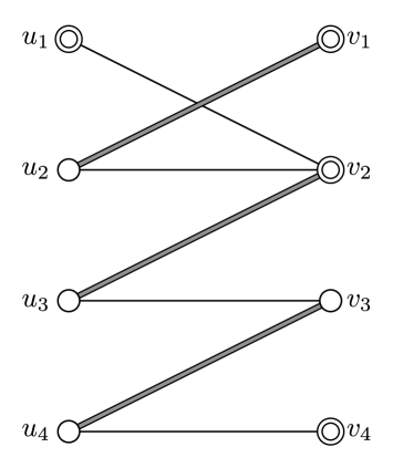
Figure 3: An illustration of starting vertices and maximal augmenting paths in $G[1,3]$. The plain edges denote unmatched edges; the shaded edges are matched. The haloed vertices have zero $y$-values. The set of starting vertices is $\{u_{1},v_{1},v_{2}\}$. The path $P=(v_{2},u_{3},v_{3},u_{4},v_{4})$ is an augmenting path but not a maximal augmenting path, since it can be extended to a longer one. For example, $(u_{1},v_{2},u_{3},v_{3},u_{4},v_{4})$ and $(v_{1},u_{2},v_{2},u_{3},v_{3},u_{4},v_{4})$ are augmenting paths containing $P$.

In the second stage of augmentation we will eliminate all the augmenting paths in $G[1,3]$. This is done by finding a maximal set of vertex-disjoint maximal augmenting paths, which are those not properly contained in another augmenting path. (Recall that in Phase II, augmenting paths can end at matched edges so long as the endpoints of the path have zero $y$-values. Any augmenting path with free endpoints is necessarily maximal, but one ending in matched edges may not be maximal.) See Figure 3 for an illustration.

Consider the graph $\vec{G}[1,3]$. It must be a directed acyclic graph, since, by Lemma 11, $G[1,3]$ does not contain augmenting cycles. Call a vertex with zero $y$-value a starting vertex if it is left and free or right and matched, and an ending vertex if it is left and matched or right and free. Let $A$ and $B$ be the set of starting and ending vertices. It follows that any augmenting path in $G[1,3]$ corresponds to a directed path from an $A$-vertex to a $B$-vertex in $\vec{G}[1,3]$. With this observation in hand we can find a maximal set $\mathcal{P}$ of maximal augmenting paths using DFS. We initiate the search on each $A$-vertex $u$ in topological order. When an augmenting path to a $B$-vertex, say $v$, is first discovered we cannot commit $(u,\ldots,v)$ to $\mathcal{P}$ immediately. Rather, we continue to look for an even longer augmenting path, and keep $(u,\ldots,v)$ only after all outgoing edges from $v$ have been exhausted. Algorithm 3 gives the Path-Search procedure.

  All vertices are initially unmarked

  $A\leftarrow\{u\>|\>\mbox{$y(u)=0$ and $u$ is left and free or right and matched}\}$ {starting vertices}       

  $B\leftarrow\{u\>|\>\mbox{$y(u)=0$ and $u$ is right and free or left and matched}\}$ {ending vertices}       

  $\mathcal{P}\leftarrow\emptyset$ {set of augmenting cycles discovered so far}       

  $\mathcal{S}\leftarrow()$ {DFS stack}       

  while there are still unmarked $A$-vertices do

     if $\mathcal{S}$ is empty then

        Push the first (topologically) unmarked $u_{0}\in A$ onto $\mathcal{S}$.

     end if

     $u$ = the top of $\mathcal{S}$

     $V_{u}=\{v\>|\>\mbox{$(u,v)\in E(\vec{G}[1,3])$ and $v$ is unmarked}\}$

     if $V_{u}$ is empty then

        if $u\in B$ then

           $\mathcal{P}\leftarrow\mathcal{P}\cup\{\mathcal{S}\}$ {$\mathcal{S}$ forms a maximal augmenting path}       

           Mark all vertices in $\mathcal{S}$ and set $\mathcal{S}\leftarrow()$ {Pop all vertices off the stack}      

        else

           Mark $u$ and pop $u$ off $\mathcal{S}$

        end if

     else

        Push an arbitrary $v\in V_{u}$ onto $\mathcal{S}$

     end if

  end while

  return  $\mathcal{P}$

ALGORITHM 3 Path-Search: returns a maximal set of maximal eligible augmenting paths

Lemma 12.

After augmenting along every path in $\mathcal{P}$, the graph $G[1,3]$ contains no augmenting paths.

Proof.

Suppose that there exists an augmenting path $Q$ after the augmentation. Then, by the maximality of $\mathcal{P}$, there must be some augmenting path in $\mathcal{P}$ sharing vertices with $Q$. There can be two cases.

Case 1

There exists a $P\in\mathcal{P}$ and a $v\in P\cap Q$ that is not an endpoint of $P$. Since $P$ contains $v$ and its mate before and after augmentation, $P$ and $Q$ must share an edge, which is impossible since all edges in $P$ become ineligible after augmentation.

Case 2

Let $P$ be the first path added to $\mathcal{P}$ that intersects $Q$. Since we are not in Case 1, $P$ and $Q$ intersect at a common endpoint, say $x$. (Note that the only way this is possible is if $x$ is matched before augmentation and free afterward. If $x$ were a free endpoint of $P$ before augmentation it would be incident to a matched ineligible edge after augmentation and could therefore not be an endpoint of $Q$.) Let $x_{P}$ and $x_{Q}$ be the other endpoints of $P$ and $Q$. If $x_{P}=x_{Q}$ then $G[1,3]$ contained an augmenting cycle, contradicting Lemma 11. If $x_{P}\in A$ is a starting vertex, consider the moment when the stack contained only $x_{P}$. At this time $PQ$ is an augmenting path of unmarked vertices, so Path-Search would not place the non-maximal augmentation $P$ in $\mathcal{P}$. On the other hand, if $x$ is a starting vertex, it must be a right matched vertex that becomes free after augmentation, which implies that $x_{Q}$ must also be a starting vertex. Since our search explores $A$-vertices in topological order, the search from $x_{Q}$ would have preceded the search from $x$. Thus, the first augmentation of $\mathcal{P}$ intersecting $Q$ must contain $x_{Q}$, contradicting the fact that $P$ does not contain $x_{Q}$.

∎

4.4 Phase II Dual Adjustment

Recall that scale $i$ ends when $M\subseteq G[0,1]$. Let $B=M\cap G[2,3]$ be the bad edges and let $f:E\rightarrow\{0,1,2\}$ measure the badness, defined as follows.

$$f(e)=\left\{\begin{array}[]{ll}\frac{y(e)-w_{i}(e)-\delta_{i}}{\delta_{i}}&\mbox{ for $e\in B$}\\ 0&\mbox{ for $e\not\in B$}\end{array}\right.$$

Let $f(M)=\sum_{e\in B}f(e)$ be the total badness of $M$. The goal of dual adjustment is to eliminate $B$, or equivalently, to reduce $f(M)$ to 0. We will show how to reduce $f(M)$ by roughly $\sqrt{f(M)}$ in linear time.

A $B^{\prime}\subseteq B$ is called a chain if there is an alternating path in $G[1,3]$ containing $B^{\prime}$ and an anti-chain if no alternating path in $G[1,3]$ contains two edges $e_{1},e_{2}\in B^{\prime}$. Lemma 13 basically follows from Dilworth’s lemma [22].

Lemma 13.

For any $t>1$, there exists $B^{\prime}\subseteq B$ such that either $B^{\prime}$ is a chain with $f(B^{\prime})\geq\lceil t\rceil$ or $B^{\prime}$ is an anti-chain with $|B^{\prime}|\geq\lceil f(M)/2t\rceil$. Moreover, such a $B^{\prime}$ can be found in linear time.

Proof.

Let $S$ be the set of vertices with zero in-degree in the acyclic graph $\vec{G}[1,3]$. In linear time we compute distances from $S$ using $-f$ as the length function. Let $d(v)$ be the distance to $v$. Suppose there is a $v$ with $d(v)\leq-\lceil t\rceil$ and let $P$ be a shortest path to $v$. It follows that $B^{\prime}=P\cap B$ is a chain with $f(B^{\prime})\geq\lceil t\rceil$. If this is not the case then, for every $(u,v)\in B$ (where $v$ is a left vertex), $d(v)\in[-(\lceil t\rceil-1),-1]$. Since $f(e)\leq 2$ for $e\in B$, we must have at least $\lceil|B|/(\lceil t\rceil-1)\rceil>\lceil f(M)/2t\rceil$ such $v$ with a common distance, say $-k$. It follows that $B^{\prime}=\{(u,v)\in B\>|\>\mbox{$v$ is a left vertex and $d(v)=-k$}\}$ is an anti-chain, for if $(u_{1},v_{1}),(u_{2},v_{2})\in B^{\prime}$ were on an alternating path in $G[1,3]$, the distance to $v_{2}$ would be strictly smaller than the distance to $v_{1}$. ∎

Below we show that if $B^{\prime}$ is a chain we can decrease the total badness by $f(B^{\prime})$ in linear time. On the other hand, if $B^{\prime}$ is an anti-chain, then we can decrease the total badness by $|B^{\prime}|/2$, also in linear time.

4.4.1 Phase II Dual Adjustment: Antichain Case

When performing dual adjustments we must be careful to maintain Property 3, which states that $y(u)$ must always be nonnegative, and must be zero if $u$ is free. This motivates the definition of a dual adjustable vertex.

Definition 4.

A vertex $u$ is said to be dual adjustable if every vertex in $V_{\operatorname{odd}}(u,G[1,3])$ is matched and every vertex $v\in V_{\operatorname{even}}(u,G[1,3])$ has $y(v)>0$.

Lemma 14.

For every $e=(u,v)\in B$, either $u$ is adjustable or $v$ is adjustable or both. Furthermore, all adjustable vertices can be found in $O(m)$ time.

Proof.

First, suppose that for some $e=(u,v)\in B$, both $u$ and $v$ are not adjustable. There must exist vertices $w$ and $x$ having zero $y$-values where $(w,\ldots,u,v,\ldots,x)$ is an augmenting path in $G[1,3]$. However, this contradicts Lemma 12, which states that there are no augmentations in $G[1,3]$ after an augmentation step. Let $\tilde{V}=\{v\>|\>\mbox{$v$ is free or $(v,v^{\prime})\in M$ and $y(v^{\prime})=0$}\}$. By definition a vertex is not dual adjustable if and only if it lies in $V_{\operatorname{odd}}(\tilde{V},G[1,3])$, which can be computed in linear time. ∎

Let $B^{\prime}\subseteq B$ be an anti-chain. The procedure Antichain-Adjust$(B^{\prime})$ selects a set of dual adjustable vertices $X$ incident to $B^{\prime}$ and on a common side (left or right), then does a dual adjustment starting at $X$. Since, by Lemma 14, for any $(u,v)\in B^{\prime}$ either $u$ is adjustable or $v$ is adjustable or both, we can guarantee that $|X|\geq|B^{\prime}|/2$. See Figure 4 for an example.

  

  Find adjustable vertices:

  $\tilde{V}\leftarrow\{v\>|\>\mbox{ $v$ is free or $(v,v^{\prime})\in M$ and $y(v^{\prime})=0$}\}$.

  Mark vertices in $V\setminus V_{\operatorname{odd}}(\tilde{V},G[1,3])$ as adjustable.

  $X_{L}\leftarrow\{u\>|\>\mbox{ $(u,v)\in B^{\prime}$ and $u$ is a left adjustable vertex}\}$,

$X_{R}\leftarrow\{u\>|\>\mbox{ $(u,v)\in B^{\prime}$ and $u$ is a right adjustable vertex}\}$.

  If $|X_{R}|\geq|X_{L}|$, then let $X\leftarrow X_{R}$; otherwise let $X\leftarrow X_{L}$.

  

  Perform dual adjustments, starting at $X$:

  $y(v)\leftarrow\begin{cases}y(v)-\delta_{i}&\mbox{if $v\in V_{\operatorname{even}}(X,G[1,3])$}\\ y(v)+\delta_{i}&\mbox{if $v\in V_{\operatorname{odd}}(X,G[1,3])$}\\ y(v)&\mbox{otherwise}\end{cases}$

ALGORITHM 4 Antichain-Adjust$(B^{\prime})$

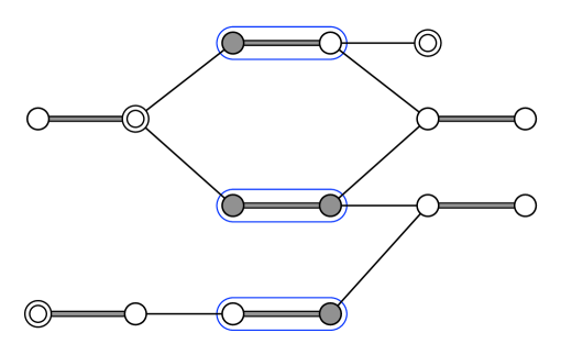
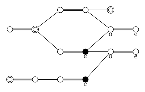
(a)	(b)

Figure 4: (a) The haloed vertices have zero $y$-values. The circled matched edges form an antichain $B^{\prime}$. The shaded vertices in $V(B^{\prime})$ are dual adjustable. (b) The black vertices are in $X$ and vertices marked with ‘e’ and ‘o’ are in $V_{\operatorname{even}}(X,G[1,3])$ and $V_{\operatorname{odd}}(X,G[1,3])$, respectively.

Lemma 15.

The dual adjustment starting at $X$ will not break Property 3(1,2,4). Furthermore, it makes Property 3(3) tighter by decreasing $f(M)$ by $|X|$.

Proof.

Since $X$ consists of adjustable vertices, every vertex $v\in V_{\operatorname{even}}(X,G[1,3])$ must have $y(v)>0$, implying $y(v)$ will be non-negative after being decremented by $\delta_{i}$. Thus, Property 3(1) is maintained. Furthermore, $V_{\operatorname{odd}}(X,G[1,3])$ cannot contain a free vertex, which implies that Property 3(4) is preserved. Since all vertices in $X$ are on the same left/right side, $y(e)$ can change by at most $\delta_{i}$. Property 3(2) (domination) is maintained since no tight edge (with $y(e)=w_{i}(e)$) can can have one endpoint in $V_{\operatorname{even}}(X,G[1,3])$ without the other being in $V_{\operatorname{odd}}(X,G[1,3])$. The algorithm does not increase $f(M)$ since, for any $e\in M\cap G[1,3]$, if one endpoint of $e$ appears in $V_{\operatorname{odd}}(X,G[1,3])$, the other must appear in $V_{\operatorname{even}}(X,G[1,3])$. Furthermore, the algorithm decreases $f(M)$ by at least $|X|\geq|B^{\prime}|/2$ since $f(u,v)$ is decremented for each $(u,v)\in B^{\prime}$ with $v\in X$. To see this, note that $y(v)$ is decremented by $\delta_{i}$ and, since $\vec{G}[1,3]$ is acyclic and $B^{\prime}$ is an antichain, $u$ cannot appear in $V_{\operatorname{odd}}(X,G[1,3])$ and therefore cannot have its $y$-value adjusted. ∎

Therefore, by doing the dual adjustment starting at $X$, we can decrease $f(M)$ by at least $|B^{\prime}|/2$.

4.4.2 Phase II Dual Adjustment: Chain Case

In the chain case we are given a chain $B^{\prime}\subseteq B$ and a minimal alternating path $P$ containing $B^{\prime}$, that is, it starts and ends with $B^{\prime}$-edges. Setting $M\leftarrow M\oplus P$ immediately reduces $f(M)$ by $f(B^{\prime})$ since $B^{\prime}$-edges are replaced by tight edges, which contribute nothing to $f(M)$. However, the endpoints of $P$, say $u$ and $v$, are now free while possibly having positive $y$-values, which violates Property 3(4). Our goal is to restore Property 3, either by finding augmenting paths that rematch $u$ and $v$ or by reducing their $y$-values to zero. In this section an augmenting path is one in the eligibility graph $G[0,3]$ (not $G[1,3]$) that either connects $u$ and $v$ or connects an $x\in\{u,v\}$ to a vertex with zero $y$-value. A notable degenerate case is when $y(x)=0$, in which case the empty path is an augmenting path from $x$ to $x$. We begin by performing dual adjustments (as in a Hungarian search) until an augmenting path $P_{u}$ in $G[0,3]$ containing $u$ emerges. We do not augment along $P_{u}$ immediately but perform a second search for an augmenting path $P_{v}$ containing $v$. If $P_{u}$ and $P_{v}$ do not intersect we let $Q=P_{u}\cup P_{v}$. On the other hand, if $P_{u}$ and $P_{v}$ do intersect then there must be an augmenting path $P_{uv}$ between $u$ and $v$ in $G[0,3]$; we let $Q=P_{uv}$. In either case we augment along $Q$, setting $M\leftarrow M\oplus Q$. Figure 5 illustrates the case where $Q=P_{uv}$.

The search from $x\in\{u,v\}$ works as follows. If there exists an augmenting path $P_{x}$ in $G[0,3]$ starting at $x$, then return $P_{x}$. (This will be the empty path if $y(x)=0$.) Otherwise update $y$-values as follows:

$$y(z)\leftarrow\begin{cases}y(z)-\delta_{i}&\mbox{if $z\in V_{\operatorname{even}}(x,G[0,3])$}\\ y(z)+\delta_{i}&\mbox{if $z\in V_{\operatorname{odd}}(x,G[0,3])$}\\ y(z)&\mbox{otherwise}\end{cases}$$

and continue to perform these dual adjustments until an augmenting path starting from $x$ emerges. As in standard Hungarian search, this process is reducible to single source shortest paths on a non-negatively weighted directed graph. The graph is either $\vec{G}$ or its transpose, depending on the left/right side of $x$. The weight function $\hat{w}$ is zero on $M$-edges and equal to the gap between $y$-value and weight on non-$M$ edges: $\hat{w}(e)=y(e)-w_{i}(e)$. By Property 3(2) (domination), $\hat{w}$ is non-negative. The value $h(z)$ is the sum of dual adjustments until an augmenting path emerges from $x$ to $z$. If $z$ is free and on the opposite side of $x$ then this is simply the distance from $x$ to $z$. However, if $z$ is on the same side as $x$ (and therefore matched), we need another $y(v)/\delta_{i}$ dual adjustment steps to reduce its $y$-value to zero. The pseudocode for Search$(x)$ appears below.

  Initialize the weighted graph:

  $\hat{G}\leftarrow\begin{cases}\vec{G}&\mbox{ if $x$ is a left vertex}\\ \vec{G}^{T}&\mbox{ if $x$ is a right vertex (reverse the orientation)}\end{cases}$

  $\hat{w}(e)\leftarrow\begin{cases}y(e)-w_{i}(e)&\text{if $e\notin M$}\\ 0&\text{if $e\in M$}\end{cases}$

  Compute distances. For each $z\in V$:

  $d(z)\leftarrow$ distance from $x$ to $z$ in $\hat{G}$ with respect to $\hat{w}$, or $\infty$ if $z$ is unreachable from $x$.

  $h(z)\leftarrow\begin{cases}d(z)&\text{if $z$ is free and not on the same side as $x$}\\ d(z)+y(z)&\text{if $z$ is on the same side as $x$}\\ \infty&\text{otherwise}\end{cases}$

  $z_{\min}\leftarrow\operatorname*{arg\,min}_{z\in V}\{h(z)\}$

  $\Delta\leftarrow h(z_{\min})$

  Perform dual adjustments. For each $z\in V$:

  $y(z)\leftarrow\begin{cases}y(z)-max\{0,\Delta-d(z)\}&\text{if $z$ is on the same side as $x$}\\ y(z)+max\{0,\Delta-d(z)\}&\text{if $z$ is not on the same side as $x$}\end{cases}$

  $P_{x}\leftarrow$ a shortest path from $x$ to $z_{\min}$. (Note: $\hat{w}(P_{x})=0$ after dual adjustments above.)

  return  $P_{x}$

ALGORITHM 5 Search$(x)$

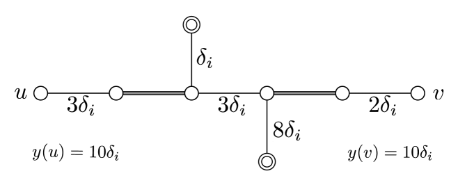
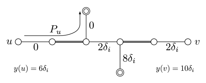
(a)	(b)
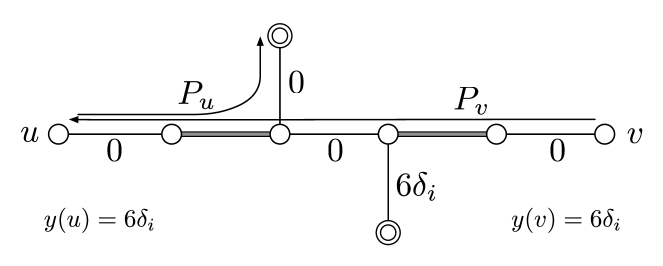
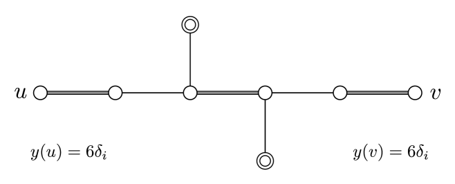
(c)	(d)

Figure 5: An example illustrating procedures for the chain case. Edges are shown with their new weight $\hat{w}$. The haloed vertices are free vertices with zero $y$-values. (a) After augmenting along $P$, $u$ and $v$ become free while having positive $y$-values. (b) search$(u)$ adjusts duals by $\Delta_{u}=4\delta_{i}$ and finds an augmenting path $P_{u}$. (c) search$(v)$ adjusts duals by $\Delta_{v}=4\delta_{i}$ and finds $P_{v}$. (d) Augmentation along $Q$. This is the case where there exists an augmenting path $Q$ between $u$ and $v$ in $G[0,3]$, which happens to be $P_{v}$ in the example.

Each execution of Search$(x)$ clearly takes linear time, except for the computation of the distance function $d$. We use Dijkstra’s algorithm [21], implementing the priority queue as an array of buckets [20]. Since $\hat{w}(e)/\delta_{i}$ is an integer and we are only interested in distances at most $\Delta$ (see the pseudocode of Search), a $(\Delta/\delta_{i})$-length array suffices. Lemma 16 implies that $\Delta=O(n\delta_{i})$, which gives a total running time of $O(m+n)$.

Lemma 16.

Augmenting along $P$ then $Q$ does not decrease the weight of the matching, that is, $w((M\oplus P)\oplus Q)\geq w(M)$. Furthermore, $\Delta_{u}+\Delta_{v}\leq 3n\delta_{i}$, where $\Delta_{x}$ is the sum of dual adjustments performed by Search$(x)$.

Proof.

Call $M_{1}=M\oplus P$ and $M_{2}=M_{1}\oplus Q$ the matchings after augmenting along $P$ and then $Q$ and let $\tilde{w}$ be the weight function $\tilde{w}(e)=y(e)-w_{i}(e)$. (Notice that $\tilde{w}$ differs from $\hat{w}$ on the matched edges.) For a quantity $q$ denote its value before Search$(u)$ and Search$(v)$ by $q_{old}$ and after both searches by $q_{new}$. After the two searches, we must have:

$$w_{i}(Q\setminus M_{1}) =\sum_{e\in Q\setminus M_{1}}y_{new}(e)$$ tightness on unmatched edges

$$=y_{new}(u)+y_{new}(v)+\sum_{e\in M_{1}\cap Q}y_{new}(e)$$ (6)

$$=\makebox[0.0pt][l]{$y_{new}(u)+y_{new}(v)+w_{i}(M_{1}\cap Q)+\tilde{w}_{new}(M_{1}\cap Q)$} \tilde{w}_{new}$$ defn. of

Line (6) follows since, aside from $u$ and $v$, $V(Q\setminus M_{1})$ and $V(M_{1}\cap Q)$ differ only on vertices with zero $y$-values. (These are the other endpoints of $P_{u}$ and $P_{v}$ when $Q=P_{u}\cup P_{v}$.) Therefore,

$$w_{i}(M_{2}) =w_{i}(M_{1})+w_{i}(Q\setminus M_{1})-w_{i}(M_{1}\cap Q)$$

$$=w_{i}(M_{1})+y_{new}(u)+y_{new}(v)+\tilde{w}_{new}(M_{1}\cap Q)$$ (7)

A similar proof shows that before the two searches, we have

$$w_{i}(M)=w_{i}(M_{1})+y_{old}(u)+y_{old}(v)-\tilde{w}_{old}(M\cap P)$$ (8)

The total amount of dual adjustment in both searches is at most the distance from $u$ to $v$, so $\Delta_{u}+\Delta_{v}\leq\tilde{w}_{old}(M\cap P)\leq 3n\delta_{i}$. Moreover:

$$w_{i}(M_{2}) \geq w_{i}(M_{1})+y_{new}(u)+y_{new}(v) \tilde{w}_{new}(M_{1}\cap Q)\geq 0$$ by (7) and

$$=w_{i}(M_{1})+y_{old}(u)+y_{old}(v)-\Delta_{u}-\Delta_{v}$$

$$\geq w_{i}(M_{1})+y_{old}(u)+y_{old}(v)-\tilde{w}_{old}(M\cap P)$$

$$=w_{i}(M)$$ by (8)

∎

Lemma 17.

At most $O(\sqrt{n})$ rounds of augmentation and dual adjustment are required to reduce $f(M)$ to $0$.

Proof.

We apply Lemma 13 with $t=\sqrt{b}/2$, where $b=f(M)$. It follows that in linear time we can either obtain an anti-chain $B^{\prime}$ of size at least $\lceil\sqrt{b}\rceil$ and reduce $f(M)$ by $\lceil\sqrt{b}/2\rceil$, or obtain a chain $B^{\prime}$ such that $f(B^{\prime})\geq\lceil\sqrt{b}/2\rceil$ and reduce $f(M)$ by $f(B^{\prime})$. In either case we can reduce $f(M)$ by $\lceil\sqrt{b}/2\rceil$. The number of rounds is at most $T(b)$, where $T(0)=0$ and $T(b)=T(b-\lceil\sqrt{b}/2\rceil)+1$ for $b>0$. A proof by induction shows that $T(b)\leq 4\sqrt{b}$, which is at most $4\sqrt{2n}$ since $|M|\leq n$ and $f(e)\leq 2$ for $e\in M$. ∎

Phase II concludes at the end of scale $L=\lceil\log N\rceil$, when $M\cap G[2,3]=\emptyset$. That is, when Phase III begins $y(e)=w(e)$ or $w(e)+\delta_{L}$ for each $e\in M$. (Note that $w_{L}=w$ since $\delta_{L}<1$.)

4.5 Phase III

Like a single scale of Phase II, Phase III alternately executes augmentation and dual adjustment steps. Certain complications arise since the goal of Phase III is to eliminate all non-tight $M$-edges whereas the goal of Phase II was to eliminate edges in $M\cap G[2,3]$. In order to understand the ramifications of this slight shift, we should review the interplay between augmentation and dual adjustment in Phase II. Note that Phase II augmentation steps improved the weight of $M$, but this was an incidental benefit. The real purpose of augmentation was to eliminate any augmentations in $G[1,3]$ (thereby making $\vec{G}[1,3]$ acyclic), which then let us reduce $f(M)$ by $\sqrt{f(M)}/2$ with a chain/antichain dual adjustment. The efficiency of the augmentation step stemmed from the fact that matched and unmatched edges had different eligibility criteria. Thus, augmenting along a maximal set of augmentations in $G[1,3]$ destroyed all augmentations in $G[1,3]$, that is, tight $M$-edges could and should be ignored.

In Phase III we cannot afford to exclude tight $M$-edges from the eligibility graph. This raises two concerns. First, augmenting along a maximal set of augmenting paths/cycles in $G[0,1]$ does not destroy all augmentations in $G[0,1]$. (Tight $M$-edges remain eligible after augmentation and may therefore be contained in another augmentation.) Second, $G[0,1]$ may contain cycles of tight edges, that is, augmentations that do not improve the weight of $M$, so eliminating all weight-augmenting paths/cycles does not guarantee that $\vec{G}[0,1]$ is acyclic. These concerns motivate us to redefine augmentation. In Phase III an eligible augmentation is either an alternating cycle or alternating path whose endpoints have zero $y$-values, that, in addition, is contained in $G[0,1]$ but not $G[0,0]$. That is, it cannot consist solely of tight edges.

4.5.1 Phase III Augmentation

In a Phase III Augmentation step we repeatedly augment along eligible augmentations in $G[0,1]$ until no such eligible augmentation exists. Lemma 18 lets us upper bound the aggregate time for all Phase III Augmentation steps.

Lemma 18.

An eligible augmentation $P$ in $G[0,1]$ can be found in $O(m)$ time, if one exists, and $w(M\oplus P)>w(M)$. Consequently, there can be at most $\sqrt{n}$ augmentations in Phase III.

Proof.

To find an augmentation we begin by computing the strongly connected components of $\vec{G}[0,1]$ in linear time. If the endpoints of an $e\in M\cap G[1,1]$ are in the same strongly connected component then that edge is contained in an augmenting cycle. If there are no augmenting cycles, use the linear time algorithm described in Lemma 14 to determine whether $v$ is dual adjustable for all $v\in V$. If both endpoints of some $e\in M\cap G[1,1]$ are not dual adjustable, then there must be an augmenting path containing $e$.

Let $P$ be an augmenting path or cycle. We must have $\sum_{v\in V(P\cap M)}y(v)=\sum_{v\in V(P\setminus M)}y(v)$, since the sums differ only on vertices with zero $y$-values. Thus $w(P\cap M)<\sum_{v\in V(P\cap M)}y(v)=\sum_{v\in V(P\setminus M)}y(v)=w(P\setminus M)$, where the first inequality follows from the fact that $P\cap M$ contains a non-tight edge and the last equality from the tightness of unmatched edges. Since all weights are integers, the weight of the matching is increased by at least one.

Recall that $\delta_{L}=2^{\lfloor\log N/\sqrt{n}\rfloor-\lceil\log N\rceil}\leq 1/\sqrt{n}$. By Lemma 10, we have $w(M)\geq w(M^{*})-n\delta_{L}\geq w(M^{*})-\sqrt{n}$ at the end of Phase II, where $M^{*}$ is the mwm. As in Phase II, Phase III dual adjustments will not reduce the weight of $M$. (See Lemma 16.) Since each augmentation increases the weight of $M$ there can be at most $\sqrt{n}$ augmentations in Phase III. ∎

Lemma 18 implies that the time for $\ell$ Phase III Augmentation steps is $O(\ell m+m\sqrt{n})$: linear time per step plus linear time per augmentation discovered.

4.5.2 Phase III Dual Adjustment

Since the goal of Phase III is to eliminate edges in $M\cap G[1,1]$ (as opposed to $M\cap G[2,3]$) we must redefine the badness of an edge accordingly. Let $B=M\cap G[1,1]$ be the bad edges and let $f:E\rightarrow\{0,1\}$ measure badness, where $f(e)=(y(e)-w(e))/\delta_{L}$ if $e\in B$ and zero if $e\not\in B$. We define $B^{\prime}\subseteq B$ to be a chain or antichain exactly as in Phase II. The difference is that $\vec{G}[0,1]$ is not necessarily acyclic so finding a chain or antichain requires one extra step.

Lemma 19.

For any $t>1$, there exists a $B^{\prime}\subseteq B$ such that $B^{\prime}$ is a chain with $f(B^{\prime})\geq\lceil t\rceil$ or $B^{\prime}$ is an antichain with $|B^{\prime}|=f(B^{\prime})\geq\lceil f(M)/t\rceil$. Moreover, $B^{\prime}$ can be found in linear time.

Proof.

Let $\vec{G}^{*}$ be the graph obtained from $\vec{G}[0,1]$ by contracting all strongly connected components in $\vec{G}[0,0]$. Since $G[0,1]$ contains no eligible augmenting cycles after a Phase III Augmentation step, all $B$-edges straddle different strongly connected components and therefore remain in $\vec{G}^{*}$. By definition $\vec{G}^{*}$ is acyclic. The argument from Lemma 13 shows that $\vec{G}^{*}$ contains a chain $B^{\prime}$ with $f(B^{\prime})\geq\lceil t\rceil$ or an antichain with $|B^{\prime}|=\lceil f(M)/t\rceil$, and that such a $B^{\prime}$ can be found in linear time. ∎

We can apply the chain and antichain elimination procedures from Phase II without compromising correctness since Lemmas 14, 15, 16, and 17 remain valid if we substitute $G[0,1]$ for $G[1,3]$. Let $t=\sqrt{b/2}$, where $b=f(M)$ is the current total badness. Lemmas 14 and 19 imply that we can reduce $f(M)$ by $\lceil t\rceil\geq\sqrt{b/2}$ in the chain case or $\lceil b/2t\rceil\geq\sqrt{b/2}$ in the antichain case. The number of augmentation and dual adjustment steps in Phase III is then $T(b)$ where $T(b)=T(b-\lceil\sqrt{b/2}\rceil)+1$ and $T(0)=0$. By induction $T(b)\leq 2\sqrt{2b}$, which is at most $2\sqrt{2n}$ since $f(M)\leq n$. Thus, the total time spent on dual adjustment in Phase III is still $O(m\sqrt{n})$.

4.6 Maximum Weight Perfect Matching

Recall from Section 1 that the maximum weight perfect matching problem (mwpm) is reducible to mwm. One simply adds $nN$ to the weight of every edge; a mwm in the new graph is necessarily a mwpm in the original. Thus, our mwm algorithm solves the mwpm problem in $O(m\sqrt{n}\log(nN))$ time, where the number of scales is $\log((n+1)N)$. However, we can circumvent this roundabout reduction and solve mwpm directly, in $\log(\sqrt{n}N)$ scales, that is, a factor 2 improvement for small $N\ll n$. We substitute Property 4 for Property 3.

Property 4.

Redefine $\delta_{0}=2^{\lfloor\log N\rfloor}$, $L=\lceil\log(\sqrt{n}N)\rceil$. In each scale $i\in[0,L]$, we maintain a perfect matching $M$ satisfying the following properties.

1. Granularity: $y(u)$ is a multiple of $\delta_{i}$ for all $u\in V$.

2. Domination: $y(e)\geq w_{i}(e)$ for all $e\in E$.

3. Near Tightness: For any $e\in M$, $y(e)\leq w_{i}(e)+3\delta_{i}$ throughout scale $i$ and $y(e)\leq w_{i}(e)+\delta_{i}$ at the end of scale $i$.

In Phase I we find any perfect matching $M$ in $O(m\sqrt{n})$ time [65, 23, 74] and initialize $y$-values to satisfy Property 4.

$$y(u)\leftarrow\begin{cases}\delta_{0}&\mbox{ if $u$ is a left vertex}\\ 0&\mbox{ if $u$ is a right vertex}\end{cases}$$

Since $y(e)\leq w_{i}(e)+\delta_{0}$ for $e\in M$, Property 4 lets us end scale 0.

As before, Phase II operates at scales $i\in[1,L]$ and Phase III operates at scale $L$ with the following simplifications:

1. To begin scale $i$ we simply increment $y(u)$ by $\delta_{i}$ for each left vertex $u$. There is no need for an initial augmentation/dual adjustment (as in Section 4.2) since there are no free vertices.

2. As there are no free vertices, an augmentation is always an augmenting cycle. In the Phase II and Phase III augmentation steps we use only Cycle-Search, not Path-Search.

3. We do not prohibit negative $y$-values. Thus, in the antichain case of dual adjustment, both endpoints of a $B^{\prime}$-edge are dual-adjustable and we can reduce $f(M)$ by $|B^{\prime}|$ rather than just $|B^{\prime}|/2$.

4. In the chain case of dual adjustment, setting $M\leftarrow M\oplus P$ temporarily frees $P$’s endpoints, say $u$ and $v$. We execute Search$(u)$ but force $z_{\min}=v$, that is Search returns a $u$-to-$v$ path $P_{u}$. Setting $M\leftarrow M\oplus P_{u}$ restores the perfection of $M$. There is no need for Search$(u)$ to calculate $h$-values. These were introduced to maintain Property 3(1), namely that $y$-values are non-negative.

5. We change the parameter that determines whether we apply a chain or antichain dual adjustment. Choose $t=\sqrt{b/2}$, where $b=f(M)$. Either we can obtain an anti-chain $B^{\prime}$ of size at least $\lceil\sqrt{b/2}\rceil$ and decrease $f(M)$ by $\lceil\sqrt{b/2}\rceil$, or we can obtain a chain $B^{\prime}$ such that $f(B^{\prime})\geq\lceil\sqrt{b/2}\rceil$ and decrease $f(B)$ by $f(B^{\prime})$. Thus, the number of rounds is at most $T(b)=T(b-\lceil\sqrt{b}/2\rceil)+1\leq 2\sqrt{2b}$. In a Phase II scale $b\leq 2n$, so $4\sqrt{n}$ augmentation/dual adjustment steps are needed. In Phase III $b\leq n$ so $2\sqrt{2n}$ steps are needed.

6. Note that since $\delta_{L}=2^{\lfloor\log N\rfloor-\lceil\log(\sqrt{n}N)\rceil}\leq 1/\sqrt{n}$, at the end of Phase II we have $w(M)\geq w(M^{*})-n\delta_{L}\geq w(M^{*})-\sqrt{n}$, by Lemma 10. Thus, the matching can be augmented at most $\sqrt{n}$ times in Phase III and the total time spent in augmentation steps is $O(m\sqrt{n})$.

The main difference between our mwm and mwpm algorithms is in Phase I. In the mwm algorithm we can afford to use a smaller value for $\delta_{0}$ since Phase I ends when free vertices have zero $y$-values, whereas Phase I of the mwpm algorithm ends only when we have a perfect matching.

References

- [1] P. K. Agarwal and K. R. Varadarajan. A near-linear constant-factor approximation for Euclidean bipartite matching? In Proceedings 20th ACM Symposium on Computational Geometry, pages 247–252, 2004.
- [2] H. Alt, N. Blum, K. Mehlhorn, and M. Paul. Computing a maximum cardinality matching in a bipartite graph in time . Info. Proc. Lett., 37(4):237–240, 1991.
- [3] T. Anderson, S. Owicki, J. Saxe, and C. Thacker. High speed switch scheduling for local area networks. ACM Trans. Comput. Syst., 11(4):319–352, 1993.
- [4] A. Andersson, T. Hagerup, S. Nilsson, and R. Raman. Sorting in linear time? J. Comput. Syst. Sci., 57(1):74–93, 1998.
- [5] D. Avis. Two greedy heuristics for the weighted matching problems. In Proceedings 9th Southeast Conference on Combinatorics, Graph Theory, and Computing (Congr. Numer. XXI), pages 65–76, 1978.
- [6] D. Avis. A survey of heuristics for the weighted matching problem. Networks, 13:475–493, 1983.
- [7] M. L. Balinski. Labelling to obtain a maximum matching. In R. C. Bose and T. A. Downing, editors, Combinatorial Mathematics and its Applications, pages 585–602. University of North Carolina Press, 1969.
- [8] M. L. Balinski and R. E. Gomory. A primal method for the assignment and transportation problems. Management Science, 10(3):578–593, 1964.
- [9] D. .P. Bertsekas. A new algorithm for the assignment problem. Mathematical Programming, 21:152–171, 1981.
- [10] G. Birkhoff. Tres observaciones sobre el elgebra lineal. Universidad Nacional de Tucuman, Revista A, 5(1–2):147–151, 1946.
- [11] H. E. Brogden. An approach to the problem of differential prediction. Psychometrika, 11(3):139–154, 1946.
- [12] G. Brown and J. von Neumann. Solutions of games by differential equations. In H. Kuhn and A. Tucker, editors, Contributions to the Theory of Games, volume 24 of Annals of Mathematical Studies, pages 73–79. Princeton University Press, 1950.
- [13] M. Charikar. Similarity estimation techniques from rounding algorithms. In Proceedings 34th ACM Symposium on Theory of Computing (STOC), pages 380–388, 2002.
- [14] J. Cheriyan and K. Mehlhorn. Algorithms for dense graphs and networks on the random access computer. Algorithmica, 15(6):521–549, 1996.
- [15] N. Christofides. Worst case analysis of a new heuristic for the travelling salesman problem. Technical report, Graduate School of Industrial Administration, Carnegie Mellon University, 1976.
- [16] R. Cole, R. Hariharan, M. Lewenstein, and E. Porat. A faster implementation of the Goemans-Williamson clustering algorithm. In Proceedings 12th ACM-SIAM Symposium on Discrete Algorithms (SODA), pages 17–25, 2001.
- [17] W. H. Cunningham and A. B. Marsh, III. A primal algorithm for optimum matching. Mathematical Programming Study, 8:50–72, 1978.
- [18] G. B. Dantzig. Application of the simplex method to the transportation problem. In T. C. Koopmans, editor, Activity Analysis of Production and Allocation, Cowles Commission Monograph 13, pages 359–373. John Wiley and Sons, New York, 1951.
- [19] J. F. Desler and S. L. Hakimi. A graph-theoretic approach to a class of integer-programming problems. Operations Research, 17(6):1017–1033, 1969.
- [20] R. B. Dial. Algorithm 360: shortest-path forest with topological ordering. Comm. ACM, 12(11):632–633, 1969.
- [21] E. W. Dijkstra. A note on two problems in connexion with graphs. Numerische Mathematik, 1:269–271, 1959.
- [22] R. P. Dilworth. A decomposition theorem for partially ordered sets. The Annals of Mathematics, 51(1):161–166, 1950.
- [23] E. A. Dinic. Algorithm for solution of a problem of maximum flow in networks with power estimation. Soviet Math. Dokl., 11:1277–1280, 1970.
- [24] E. A. Dinic and M. A. Kronrod. An algorithm for the solution of the assignment problem. Soviet Math. Dokl., 10(6):1324–1326, 1969.
- [25] D. Drake and S. Hougardy. Improved linear time approximation algorithms for weighted matchings. In 7th International Workshop on Randomization and Approximation Techniques in Computer Science (APPROX), LNCS 2764, pages 14–23, 2003.
- [26] D. Drake and S. Hougardy. A simple approximation algorithm for the weighted matching problem. Info. Proc. Lett., 85:211–213, 2003.
- [27] R. Duan and S. Pettie. Approximating maximum weight matching in near-linear time. In Proceedings 51st IEEE Symposium on Foundations of Computer Science (FOCS), pages 673–682, 2010.
- [28] I. S. Duff and J. R. Gilbert. Maximum-weighted matching and block pivoting for symmetric indefinite systems. In Householder Symposium XV Book of Abstracts, pages 73–75, 2002.
- [29] T. E. Easterfield. A combinatorial algorithm. J. London Math. Soc., 21:219–226, 1946. Republished as: An algorithm for the allocation problem, Operations Research 11, 3, pp. 123–129, 1960.
- [30] J. Edmonds. Maximum matching and a polyhedron with -vertices. J. Res. Nat. Bur. Standards Sect. B, 69B:125–130, 1965.
- [31] J. Edmonds. Paths, trees, and flowers. Canadian Journal of Mathematics, 17:449–467, 1965.
- [32] J. Edmonds and E. L. Johnson. Matching, Euler tours, and the Chinese postman. Mathematical Programming, 5:88–124, 1973.
- [33] J. Edmonds and R. M. Karp. Theoretical improvements in algorithmic efficiency for network flow problems. J. ACM, 19(2):248–264, 1972.
- [34] T. Feder and R. Motwani. Clique partitions, graph compression and speeding-up algorithms. J. Comput. Syst. Sci., 51(2):261–272, 1995.
- [35] L. R. Ford and D. R. Fulkerson. Flows in Networks. Princeton University Press, 1962.
- [36] M. L. Fredman and R. E. Tarjan. Fibonacci heaps and their uses in improved network optimization algorithms. J. ACM, 34(3):596–615, 1987.
- [37] M. L. Fredman and D. E. Willard. Surpassing the information-theoretic bound with fusion trees. J. Comput. Syst. Sci., 47(3):424–436, 1993.
- [38] H. N. Gabow. Implementation of algorithms for maximum matching on nonbipartite graphs. Ph.D. thesis, Stanford University, 1974.
- [39] H. N. Gabow. Scaling algorithms for network problems. In Proceedings 24th IEEE Symposium on Foundations of Computer Science (FOCS), pages 248–257, 1983.
- [40] H. N. Gabow. A scaling algorithm for weighted matching on general graphs. In Proceedings 26th IEEE Symposium on Foundations of Computer Science (FOCS), pages 90–100, 1985.
- [41] H. N. Gabow. Scaling algorithms for network problems. J. Comput. Syst. Sci., 31(2):148–168, 1985.
- [42] H. N. Gabow. Data structures for weighted matching and nearest common ancestors with linking. In Proceedings First Annual ACM-SIAM Symposium on Discrete Algorithms (SODA), pages 434–443, 1990.
- [43] H. N. Gabow, Z. Galil, and T. H. Spencer. Efficient implementation of graph algorithms using contraction. J. ACM, 36(3):540–572, 1989.
- [44] H. N. Gabow and S. Pettie. The dynamic vertex minimum problem and its application to clustering-type approximation algorithms. In Proceedings 8th Scandinavian Workshop on Algorithm Theory (SWAT), pages 190–199, 2002.
- [45] H. N. Gabow and R. E. Tarjan. Almost-optimum speed-ups for bipartite matching and related problems. In Proceedings 20th Annual ACM Symposium on Theory of Computing (STOC), pages 514–527, 1988.
- [46] H. N. Gabow and R. E. Tarjan. Faster scaling algorithms for network problems. SIAM J. Comput., 18(5):1013–1036, 1989.
- [47] H. N. Gabow and R. E. Tarjan. Faster scaling algorithms for general graph-matching problems. J. ACM, 38(4):815–853, 1991.
- [48] Z. Galil, S. Micali, and H. N. Gabow. An algorithm for finding a maximal weighted matching in general graphs. SIAM J. Comput., 15(1):120–130, 1986.
- [49] P. Giaccone, E. Leonardi, and D. Shah. On the maximal throughput of networks with finite buffers and its application to buffered crossbars. In Proceedings 24th INFOCOM, volume 2, pages 971–980, 2005.
- [50] A. Gleyzal. An algorithm for solving the transportation problem. J. Res. Nat. Bur. Standards, 54(4):213–216, 1955.
- [51] M. X. Goemans and D. P. Williamson. A general approximation technique for constrained forest problems. SIAM J. Comput., 24(2):296–317, 1995.
- [52] A. V. Goldberg. Scaling algorithms for the shortest paths problem. SIAM J. Comput., 24(3):494–504, 1995.
- [53] A. V. Goldberg and A. V. Karzanov. Maximum skew-symmetric flows and matchings. Math. Program., Ser. A, 100:537–568, 2004.
- [54] A. V. Goldberg and R. Kennedy. Global price updates help. SIAM J. Discrete Mathematics, 10(4):551–572, 1997.
- [55] F. Hadlock. Finding a maximum cut of a planar graph in polynomial time. SIAM J. Comput., 4(3):221–225, 1975.
- [56] M. Hagemann and O. Schenk. Weighted matchings for preconditioning symmetric indefinite linear systems. SIAM J. Sci. Comput., 28(2):403–420, 2006.
- [57] Yijie Han. Deterministic sorting in time and linear space. In Proceedings 34th ACM Symposium on Theory of Computing (STOC), pages 602–608. ACM Press, 2002.
- [58] S. Hanke. Zwei approximative Algorithmen für das Matchingproblem in gewichteten Graphen. PhD thesis, Humboldt-Universität zu Berlin, 2004.
- [59] S. Hanke and S. Hougardy. New approximation algorithms for the weighted matching problem. Research Report No. 101010, Research Institute for Discrete Mathematics, University of Bonn, 2010.
- [60] N. Harvey. Algebraic algorithms for matching and matroid problems. SIAM J. Comput., 39(2):679–702, 2009.
- [61] B. Hendrickson and R. Leland. The Chaco user’s guide: Version 2.0. Technical Report SAND94–2344, Sandia National Laboratories, 1995.
- [62] F. L. Hitchcock. The distribution of a product from several sources to numerous localities. J. Math. Physics, 20:224–230, 1941.
- [63] A. J. Hoffman and H. M. Markowitz. A note on shortest path, assignment, and transportation problems. Naval Research Logistics Quarterly, 10(1):375–379, 1963.
- [64] M. Holtgrewe, P. Sanders, and C. Schulz. Engineering a scalable high quality graph partitioner. In Proceedings 24th IEEE Symposium on Parallel and Distributed Processing (IPDPS), pages 1–12, 2010.
- [65] J. E. Hopcroft and R. M. Karp. An algorithm for maximum matchings in bipartite graphs. SIAM J. Comput., 2:225–231, 1973.
- [66] C.-C. Huang and T. Kavitha. Efficient algorithms for maximum weight matchings in general graphs with small edge weights. In Proceedings ACM-SIAM 23rd Symposium on Discrete Algorithms (SODA), pages ??–??, 2012.
- [67] O. H. Ibarra and S. Moran. Deterministic and probabilistic algorithms for maximum bipartite matching via fast matrix multiplication. Info. Proc. Lett., 13(1):12–15, 1981.
- [68] P. Indyk. A near linear time constant factor approximation for Euclidean bichromatic matching (cost). In Proceedings 18th ACM-SIAM Symposium on Discrete Algorithms (SODA), pages 39–42, 2007.
- [69] M. Iri, K. Murota, and S. Matsui. Heuristics for planar minimum-weight perfect matchings. Networks, 13(1):67–92, 1983.
- [70] D. B. Johnson. Priority queues with update and finding minimum spanning trees. Info. Proc. Lett., 4(3):53–57, 1975.
- [71] L. Kantorovitch. On the translocation of masses. Doklady Akad. Nauk SSSR, 37:199–201, 1942.
- [72] M.-Y. Kao, T.-K. Lam, W.-K. Sung, and H.-F. Ting. A decomposition theorem for maximum weight bipartite matchings. SIAM J. Comput., 31(1):18–26, 2001.
- [73] G. Karypis and V. Kumar. A fast and high quality multilevel scheme for partitioning irregular graphs. SIAM J. Sci. Comput., 20(1):359–392, 1998.
- [74] A. V. Karzanov. An exact estimate of an algorithm for finding a maximum flow, applied to the problem “on representatives” [in Russian]. Problems in Cybernetics, 5:66–70, 1973. Announced at the Seminar on Combinatorial Mathematics (Moscow, 1971). English translation available at the author’s website.
- [75] A. V. Karzanov. Efficient implementations of Edmonds’ algorithms for finding matchings with maximum cardinality and maximum weight. In A. A. Fridman, editor, Studies in Discrete Optimization, pages 306–327. Nauka, Moscow, 1976.
- [76] H. W. Kuhn. The Hungarian method for the assignment problem. Naval Research Logistics Quarterly, 2:83–97, 1955.
- [77] H. W. Kuhn. On combinatorial properties of matrices. George Washington University Logistics Papers, 11:1–11, 1955. English translation of J. Egerváry, Matrixok kombinatorius tulajdonságairól, Matematikai és Fizikai Lapok 38, 16–28, 1931.
- [78] H. W. Kuhn. Variants of the Hungarian method for assignment problems. Naval Research Logistics Quarterly, 3:253–258 (1957), 1956.
- [79] H. W. Kuhn and W. J. Baumol. An approximate algorithm for the fixed-charges transportation problem. Naval Research Logistics Quarterly, 9:1–15, 1962.
- [80] J. M. Kurtzberg. On approximation methods for the assignment problem. J. ACM, 9(4):419–439, 1962.
- [81] M. K. Kwan. Graphic programming using odd or even points. Chinese Mathematics, 1:273–277, 1962.
- [82] E. Lawler. Combinatorial Optimization: Networks and Matroids. Holt, Rinehart & Winston, New York, 1976.
- [83] E. Leonardi, M. Mellia, F. Neri, and M. A. Marsan. Bounds on delays and queue lengths in input-queued cell switches. J. ACM, 50(4):520–550, 2003.
- [84] N. McKeown. The iSLIP scheduling algorithm for input-queued switches. IEEE/ACM Transactions on Networking, 7(2):188–201, 1999.
- [85] N. McKeown, V. Anantharam, and J. C. Walrand. Achieving 100% throughput in an input-queued switch. In Proceedings 15th INFOCOM, pages 296–302, 1996.
- [86] S. Micali and V. V. Vazirani. An algorithm for finding maximum matching in general graphs. In Proceedings 21st IEEE Symposium on Foundations of Computer Science (FOCS), pages 17–27, 1980.
- [87] T. S. Motzkin. The assignment problem. Proceedings of Symposia in Applied Mathematics, VI, Numerical Analysis:109–125, 1956.
- [88] M. Mucha and P. Sankowski. Maximum matchings via Gaussian elimination. In Proceedings 45th IEEE Symposium on Foundations of Computer Science (FOCS), pages 248–255, 2004.
- [89] J. Munkres. Algorithms for the assignment and transportation problems. J. Soc. Indust. Appl. Math., 5:32–38, 1957.
- [90] F. Ollivier. Looking for the order of a system of arbitrary ordinary differential equations. Appl. Algebra Eng. Commun. Comput., 20(1):7–32, 2009. English translation of: C. G. J. Jacobi, De investigando ordine systematis aequationum differentialum vulgarium cujuscunque, Borchardt Journal für die reine und angewandte Mathematik 65, 4, pp. 297–320, 1865, also reproduced in: C. G. J. Jacobi, Gesammelte Werke, Vol. 5, K. Weierstrass, Ed., Berlin, Bruck und Verlag von Georg Reimer, pp. 193–216, 1890.
- [91] M. Olschowka and A. Neumaier. A new pivoting strategy for Gaussian elimination. Linear Algebra and its Applications, 240:131–151, 1996.
- [92] J. B. Orlin and R. K. Ahuja. New scaling algorithms for the assignment and minimum mean cycle problems. Math. Program., 54:41–56, 1992.
- [93] G. I. Orlova and Y. G. Dorfman. Finding the maximum cut in a planar graph. Engineering Cybernetics, 10:502–506, 1972.
- [94] F. Pellegrini. SCOTCH 5.1 user’s guide. Technical report, LaBRI, 2008.
- [95] S. Pettie. Sensitivity analysis of minimum spanning trees in sub-inverse-Ackermann time. In Proceedings 16th Int’l Symposium on Algorithms and Computation (ISAAC), pages 964–973, 2005.
- [96] S. Pettie and P. Sanders. A simpler linear time approximation to maximum weight matching. Info. Proc. Lett., 91(6):271–276, 2004.
- [97] R. Preis. Linear time -approximation algorithm for maximum weighted matching in general graphs. In Proceedings 16th Symposium on Theoretical Aspects of Computer Science (STACS), LNCS 1563, pages 259–269, 1999.
- [98] R. Preis and R. Diekmann. PARTY – A software library for graph partitioning. In B. H. V. Topping, editor, Advances in Computational Mechanics with Parallel and Distributed Processing, pages 63–71. Civil-Comp Press, 1997.
- [99] E. M. Reingold and K. J. Supowit. Probabilistic analysis of divide-and-conquer heuristics for minimum weighted Euclidean matching. Networks, 13:49–66, 1983.
- [100] E. M. Reingold and R. E. Tarjan. On a greedy heuristic for complete matching. SIAM J. Comput., 10(4):676–681, 1981.
- [101] J. Robinson. On the Hamiltonian game (a traveling salesman problem). Research Memorandum 303, RAND Corporation, 1949.
- [102] P. Sanders and C. Schulz. Distributed evolutionary graph partitioning. In Proceedings 14th Workshop on Algorithm Engineering and Experiments (ALENEX), pages 43–54, 2012.
- [103] P. Sankowski. Maximum weight bipartite matching in matrix multiplication time. Theoretical Computer Science, 410(44):4480–4488, 2009.
- [104] O. Schenk, A. Wächter, and M. Hagemann. Matching-based preprocessing algorithms to the solution of saddle-point problems in large-scale nonconvex interior-point optimization. Comput. Optim. Appl., 36(2–3):321–341, 2007.
- [105] D. Shah, P. Giaccone, and B. Prabhakar. Efficient randomized algorithms for input-queued switch scheduling. IEEE Micro, 22(1):10–18, 2002.
- [106] D. Shah and M. Kopikare. Delay bounds for the approximate maximum weight matching algorithm for input queued switches. In Proceedings 21st INFOCOM, pages 1024–1031, 2002.
- [107] R. L. Thorndike. The problem of classification of personnel. Psychometrika, 15:215–235, 1950.
- [108] M. Thorup. Undirected single-source shortest paths with positive integer weights in linear time. J. ACM, 46(3):362–394, 1999.
- [109] M. Thorup. Integer priority queues with decrease key in constant time and the single source shortest paths problem. In Proceedings 35th ACM Symposium on Theory of Computing (STOC), pages 149–158, 2003.
- [110] M. Thorup. Equivalence between priority queues and sorting. J. ACM, 54(6), 2007.
- [111] N. Tomizawa. On some techniques useful for solution of transportation network problems. Networks, 1(2):173–194, 1971.
- [112] K. R. Varadarajan and P. K. Agarwal. Approximation algorithms for bipartite and non-bipartite matching in the plane. In Proceedings 10th ACM-SIAM Symposium on Discrete Algorithms (SODA), pages 805–814, 1999.
- [113] V. V. Vazirani. A theory of alternating paths and blossoms for proving correctness of the general graph maximum matching algorithm. Combinatorica, 14(1):71–109, 1994.
- [114] D. E. D. Vinkemeier and S. Hougardy. A linear-time approximation algorithm for weighted matchings in graphs. ACM Trans. on Algorithms, 1(1):107–122, 2005.
- [115] J. von Neumann. A certain zero-sum two-person game equivalent to the optimal assignment problem. In H. W. Kuhn and A. W. Tucker, editors, Contributions to the Theory of Games, volume II, pages 5–12. Princeton University Press, 1953.
- [116] C. Walshaw and M. Cross. JOSTLE: Parallel multilevel graph-partitioning software – an overview. In Mesh Partitioning Techniques and Domain Decomposition Techniques, pages 27–58, 2007.
- [117] C. Witzgall and C. T. Zahn, Jr. Modification of Edmonds’ maximum matching algorithm. J. Res. Nat. Bur. Standards Sect. B, 69B:91–98, 1965.