A generalized likelihood ratio test statistic
for Cherenkov telescope data

Abstract

Astrophysical sources of TeV gamma rays are usually established by Cherenkov telescope observations. These counting type instruments have a field of view of few degrees in diameter and record large numbers of particle air showers via their Cherenkov radiation in the atmosphere. The showers are either induced by gamma rays or diffuse cosmic ray background. The commonly used test statistic to evaluate a possible gamma-ray excess is Li and Ma (1983), Eq. 17, which can be applied to independent on- and off-source observations, or scenarios that can be approximated as such. This formula however is unsuitable if the data are taken in so-called ”wobble” mode (pointing to several offset positions around the source), if at the same time the acceptance shape is irregular or even depends on operating parameters such as the pointing direction or telescope multiplicity. To provide a robust test statistic in such cases, this paper explores a possible generalization of the likelihood ratio concept on which the formula of Li and Ma is based. In doing so, the multi-pointing nature of the data and the typically known instrument point spread function are fully exploited to derive a new, semi-numerical test statistic. Due to its flexibility and robustness against systematic uncertainties, it is not only useful for detection purposes, but also for skymapping and source shape fitting. Simplified Monte Carlo simulations are presented to verify the results, and several applications and further generalizations of the concept are discussed.

1 Introduction

The field of very-high-energy (VHE, $>100\,\mathrm{GeV}$) gamma-ray astronomy is currently in its third generation of instruments, with an advanced future project, CTA [1], already being in its preparatory phase. The currently operated systems H.E.S.S. [2], MAGIC [3] and VERITAS [4] have established more than 100 VHE sources in the sky. The acceptence of these telescope systems covers few degrees in diameter, and declines smoothly with increasing distance from the pointing position. Establishing a gamma-ray signal from an astrophysical source requires to significantly prove a gamma-ray excess over background events that typically remain dominant even after selection cuts. This background is mostly composed of diffuse hadrons, part of which appears almost identical to electromagnetic showers and has to be considered to be irreducible [5]. Besides these ”gamma-like hadrons”, the irreducible background also contains smaller fractions of diffuse electrons and gamma rays. This irreducible background, and the statistical and systematic uncertainties that come with it, are one of the main limiting factors of TeV astronomy; usually, an observational campaign for a given source either reveals one source or none, and only in few cases, or if the effort of a large scan is undertaken, additional unexpected sources are detected. Therefore, a statistical source detection technique that is both sensitive to weak sources and stable against systematic effects is of crucial importance to the field.

The standard test statistic to evaluate an excess of gamma rays from a given sky direction is Li and Ma [6], Eq. 17, which hereafter will be refered to as $S_{\mathrm{LM}}$. It was established among several alternatives they evaluated in their paper, based on the fact that this likelihood ratio test statistic was the only one that yielded a satisfyingly Gaussian null-hypothesis distribution. The formula they presented was designed to compare the event numbers of an on- and off-source observation ($N_{\mathrm{on}}$, $N_{\mathrm{off}}$), and allows for a scaling factor $\alpha$ between the effective observation times ($t_{\mathrm{on}}=\alpha\,t_{\mathrm{off}}$) to account for unequal exposures.

In modern observation practice, most Cherenkov telescope data are not taken in On/Off-mode (see Fig. 1, left), because this strategy implies a lot of observation time dedicated to empty sky regions. Also, it is prone to systematic differences between the on- and off-data caused by instabilities in electronic or atmospheric operating conditions, especially if the off-data could not be scheduled contemporaneously enough with the on-source observation. Therefore, usually the ”wobble” technique [7] is applied, in which the data are taken at two or more observation positions offset in different directions from the main target coordinates (see Fig. 1, right). In this way, each wobble set provides both on- and off-data at the same time. In its original idea, the exposure shape is considered to have some circular symmetry, and for each wobble set the off-data can be taken from the same observation, at sky positions of similar distance to the telescope pointing position (”reflected regions” [8]). In that case, the off-exposure ratio $\alpha$ is the same for all wobble data sets, and $S_{\mathrm{LM}}$ can be applied after summing up the on- and off-events of all wobble sets. This constant $\alpha$ can also be achieved approximately if the off-data are taken from hadron-like background events (”template background”, [9]), or a ring area around the source position (”ring background” [10]), both of which require also symmetry assumptions or an efficiency correction through Monte Carlo simulations of the isotropic background.

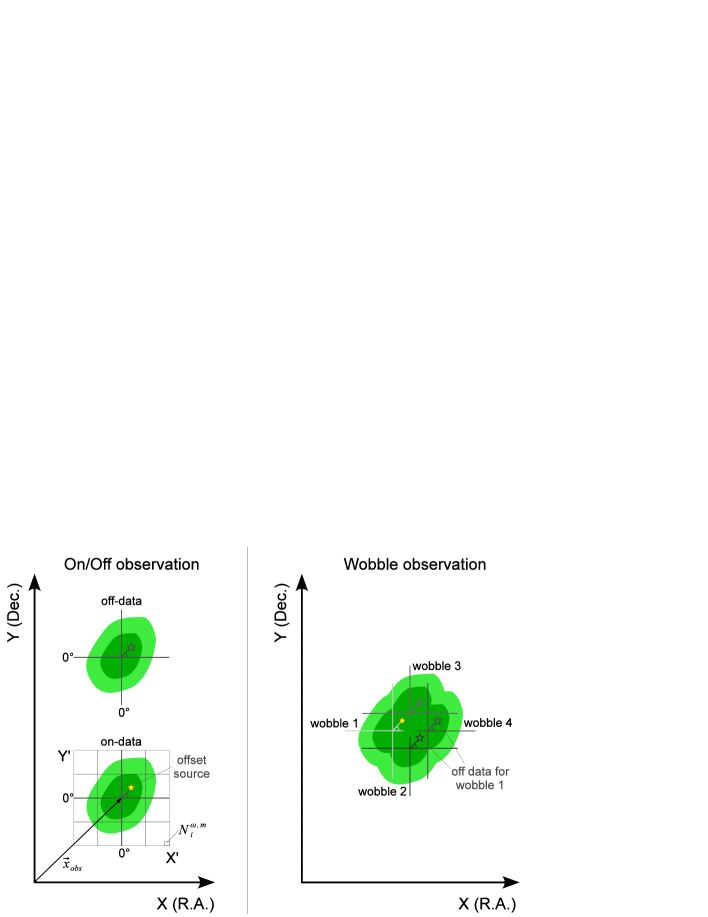
Figure 1: Observation schemes with asymmetric acceptance shapes (green areas). The sky position to be evaluated for a signal is marked with a yellow star, the corresponding off-regions with grey stars. Left: Original On/Off scheme. The off-data provides $N_{\mathrm{off}}$, the on-data $N_{\mathrm{on}}$, and it needs one exposure ratio $\alpha=t_{\mathrm{on}}/t_{\mathrm{off}}$ between those. Right: Wobble scheme with four observation positions. The off data of each wobble set can be taken from all other wobble sets, resulting in four $\alpha$ parameters and their corresponding $N_{\mathrm{on}}$, $N_{\mathrm{off}}$.

In the general case, though, the acceptance symmetry might not hold and a Monte Carlo correction may involve too high uncertainties. This occurs for instance in very low-energy observations, where camera-based acceptance inhomogeneities (dead pixels, trigger fluctuations) are both difficult to model in simulations and furthermore lead to features in the acceptance shape that can depend on the Alt/Az pointing direction or other operation parameters of the system. This is particulary troublesome in two-telescope systems like MAGIC [3], where already the basic geometrical overlap of the two fields of view implies an elongated, Alt/Az-dependent exposure shape. Under these conditions, the ”reflected regions” approach does not hold, and the off-data for each wobble set have to be taken from the other wobble sets (see Fig. 1, right). This approach can provide a sensitive measurement, because with several wobble sets, the off regions are numerous and well-populated, but it results in a different $\alpha$ for each wobble set, which is not supported by $S_{\mathrm{LM}}$. On top of that, if this procedure has to be done separately for different types of data (be it for instance different Azimuth angles or telescope multiplicities), it leads to many more $\alpha$-parameters, and in general, some off-events may happen to be oversampled if they lie in more than one off-region, which is also not considered in $S_{\mathrm{LM}}$. As a consequence, while the background density can still be modeled under certain assumptions and some numerical effort [11], the test statistic $S_{\mathrm{LM}}$, if still applied in some way, becomes very approximative. This may be dealt with in practice by making additional high requirements to the signal-to-background ratio of a detection [3], which however limits the effective sensitivity of the instrument.

Therefore, unlike previous efforts [10, 11], this work will not pursue to extract the variables needed for $S_{\mathrm{LM}}$ through the complex task of explicit background modeling. Instead, the likelihood ratio concept behind that test statistic will be generalized, and new formulae will be derived that can directly be applied to multi-wobble Cherenkov telescope data. To do so, no Monte Carlo simulations or exposure symmetry assumptions will be required. It will only be assumed that the telescope acceptance shape is the same for different wobble data sets if they are taken under similar operating conditions.

Besides that, this work will also address the disadvantage of $S_{\mathrm{LM}}$ that it depends on the size of the signal region in which $N_{\mathrm{on}}$ is calculated. This area is usually defined through an integration radius (”$\theta^{2}$-cut”, with $\theta$ being the angular distance between reconstructed gamma direction and source position). Its optimization either depends on the background density and an assumption of the source strength, or may involve several trials. In this paper, these assumptions are reduced by accomodating the knowledge of the point spread function (PSF) in the formulae, which makes them independent of the source strength or background density.

Likelihood ratios are frequently used to convert a complex likelihood maximization problem to a test statistic that follows a $\chi^{2}$-distribution. This possibility was first proven in [12], and was suggested for astronomical purposes in [13]. The technique is now widely used in counting type experiments, mainly in X-ray and gamma-ray astronomy, and can be applied both for detection and optimization purposes [14]. It should be pointed out that criticism and potentially more accurate or more general alternatives to the likelihood ratio concept exist [15, 16, 17], but are not subject of this work.

The structure of the paper is to first define the coordinate systems and naming conventions needed for the calculations. Then, a likelihood function is set up and maximized to gain all relevant parameters (Sec. 2). Based on that, the test statistic is formulated in Sec. 3 and its intrinsic inclusion of $S_{\mathrm{LM}}$ is demonstrated. In Sec. 4, some further possible generalizations and applications of the formulae are discussed and a recipe for ”Likelihood Ratio Skymapping” is suggested. Finally, some example toy simulations are shown in Sec. 5 to verify the method.

2 Building the likelihood function

In this section, a binned likelihood function is formulated which will be the basis of the likelihood ratio test statistic, but can also serve to fit the shape or positional parameters of a detected source. It is set up as a Poissonian probability function that evaluates the consistency of the different wobble subsets taken under a given operating condition with each other, allowing for a hypothetical source with a well-defined shape. It is a binned likelihood, but can be generalized to an unbinned likelihood easily (Sec. 4.5).

In this paper, the term ”operating condition” may in practice refer to a range in any quantity that influences the acceptance shape. This binning may for instance be done in the telescope pointing direction (Alt/Az) for two-telescope systems, or in the telescope multiplicity for a multi-telescope system like CTA. It may also be binned in atmospheric conditions, night sky background light level or discrete performance states of the camera. Of course, the formulae are equally valid if no such binning needs to be applied.

2.1 Namings and definitions

The data are assumed to be taken as several wobble sets $\omega=1,2,\dots,W$, centered at sky coordinates $\mathbf{x}_{\mathrm{obs},\omega}$ (”pointing directions”), throughout operating conditions $m=1,2,\dots,M$ (see previous paragraph). Hence, the observation can be described as a set of $W\times M$ two-dimensional sky histograms. These histograms shall be set up in relative sky coordinates ($\mathbf{x^{\prime}}=\mathbf{x}-\mathbf{x}_{\mathrm{obs},\omega}$) centered at the observation direction $\mathbf{x}_{\mathrm{obs},\omega}$ of each wobble set (see grid on the ”on-data” drawing of Fig. 1). The individual relative sky bins are named $i=1,2,\dots,I$, where $i$ may be regarded as a representation of a two-dimensional bin $(i_{x},i_{y})$ without loss of generality. The number of gamma-like events in one such bin $(\omega,m,i)$ is $N^{\omega,m}_{i}$. In relative sky coordinates, the shape of the background event distribution is the same for all histograms that belong to a given operating condition, while a signal at a fixed absolute sky position will appear in different relative locations for different wobble sets. In the following, the axes of the relative sky histograms ($X^{\prime}$, $Y^{\prime}$ in Fig. 1) are treated as synonyms for (relative) right ascension and declination, although in practice, one should replace those for axes that are truly rectangular throughout the field of view.

The exposure of the data taken under a given operating condition $m$ is distributed among the wobble sets $\omega$ in ratios of $a_{\omega}^{m}$, such that $\sum_{\omega}a_{\omega}^{m}=1$. There are different technical solutions of how to evaluate these ratios, the simplest and most common being through the observation times

$$a_{\omega}^{m}=\frac{t_{\omega}^{m}}{t_{\mathrm{tot}}^{m}}.$$ (1)

which is correct if the background rate is the same in all wobble sets of $m$. In the absence of a signal, the expectation value $E(N^{\omega,m}_{i})$ for a given bin ($\omega,m,i$) equals the background expectation $n^{\omega,m}_{i}$, which in turn is a well-defined fraction of the total background exposure taken under the operating condition $m$:

$$E(N^{\omega,m}_{i})=n^{\omega,m}_{i}=a_{\omega}^{m}\,n^{m}_{i}.$$ (2)

If a signal is present, its shape can be modeled with a (normalized) kernel $g^{\omega}_{i}$, which usually may be a function representing the gamma-ray PSF of the instrument, or a more extended shape for dedicated searches of extended sources. The gamma-ray PSF is usually a well-known performance characteristic that is determined from simulations and/or observations of strong known point sources. It might, as any other data cut, slightly depend on the assumed spectral index of the source. The kernel parameters $g^{\omega}_{i}$ depend on $\omega$ because the relative source coordinates depend on the wobble offset. Also, the shape of the PSF (i.e. the resolution) might depend on the distance from the pointing direction.

The kernel, which only characterizes the shape of the signal, is now multiplied by a scaling factor $\phi$ to constitute a signal term which is added to the expectation value as follows:

$$E(N^{\omega,m}_{i}\,|\,\phi)=a_{\omega}^{m}\,n^{m}_{i}\,(1\,+\,\phi\,g^{\omega}_{i})$$ (3)

This way, the excess events implied by a given relative excess $\phi$ of a source is automatically proportional to the efficiency of the detector at the position $i$ in the operating condition $m$, and to the exposure of the given wobble set $\omega$. This first-order approximation assumes that the background exposure $n^{\omega,m}_{i}$, which is proportional to the efficiency to gamma-like hadrons, is also proportional to the gamma-ray efficiency (see Sec. 4.4 for a way to loosen this assumption).

The expectation value of the relative excess $\phi$ from a gamma-ray source scales with its absolute flux. Therefore, estimators for $\phi$ can be used for flux skymapping (after the efficiency correction outlined in Sec. 4.4). Still, the meaning of $\phi$ is technically that of an excess (or deficit), and therefore it is not, like a flux, bound to be positive or zero. Also, its interpretation as a gamma-ray flux is not exclusive — a significantly non-zero excess can also be caused by other physical effects as for instance the moon shadow, or systematic detector artefacts not common to all wobble datasets. In any of these cases, the null hypothesis for the excess/deficit judgement is $\phi=0$, which is a degenerate case of the signal hypothesis, and not at the edge of the parameter space. This is important for the following, because like this, the likelihood ratio test statistic can be expected to follow a $\chi^{2}$-distribution. A remaining limitation of the $\phi$ parameter space is the fact that the expectation value for the event number, $E(N^{\omega,m}_{i}\,|\,\phi)$, has to be positive, so $\phi$ has to be larger than $-1/g^{\omega}_{\mathrm{max}}$.

While the normalization of the kernels $g^{\omega}_{i}$ has to be consistent among different $\omega$, it neither has to be unity, nor does $\sum_{i}g^{\omega}_{i}$ have to be the same for different $\omega$. For example, if additional off-observations are added to the analysis, they would have $g^{\omega}_{i}=0$ for all $i$. Also, Sec. 4.4 discusses a possible case where a varying normalization of $g^{\omega}_{i}$ is appropriate.

For convenience in the following calculations, also the averaged kernel for a given operating condition is defined:

$$g^{m}_{i}\equiv\sum_{\omega}a_{\omega}^{m}\,g^{\omega}_{i}$$ (4)

and the sum of events in a given bin $(m,i)$:

$$N^{m}_{i}\equiv\sum_{\omega}N^{\omega,m}_{i}$$ (5)

2.2 The likelihood function

The likelihood function can be defined as the product of all Poissonian probability functions of the bins in $i$, $\omega$ and $m$:

$$L(N^{\omega,m}_{i}\,|\,n^{m}_{i},\phi) =\prod_{m}\prod_{i}\prod_{\omega}\frac{(a_{\omega}^{m}\,n^{m}_{i}\,(1\,+\,\phi\,g^{\omega}_{i}))^{N^{\omega,m}_{i}}}{N^{\omega,m}_{i}!}\,e^{-a_{\omega}^{m}\,n^{m}_{i}\,(1\,+\,\phi\,g^{\omega}_{i})}$$ (6)

$$=\prod_{m}\prod_{i}e^{-n^{m}_{i}\,(1\,+\,\phi\,g^{m}_{i})}\prod_{\omega}\frac{(a_{\omega}^{m}\,n^{m}_{i}\,(1\,+\,\phi\,g^{\omega}_{i}))^{N^{\omega,m}_{i}}}{N^{\omega,m}_{i}!}$$ (7)

The latter step took advantage of the normalization of $a_{\omega}^{m}$ within each $m$ and the average kernel convention (Eq. 4).

For the maximization procedure, it is convenient to calculate the log-likelihood $\mathcal{L}=\ln L$, which is

$$\mathcal{L}(N^{\omega,m}_{i}\,|\,n^{m}_{i},\phi)=K+\sum_{m}\sum_{i}\left[-n^{m}_{i}\,(1\,+\,\phi\,g^{m}_{i})+\sum_{\omega}N^{\omega,m}_{i}\,\ln\left(n^{m}_{i}\,(1\,+\,\phi\,g^{\omega}_{i})\right)\right]$$ (8)

All terms that are independent of the free parameters $n^{m}_{i},\phi$ were absorbed into the constant $K$.

2.3 Determination of the parameters

The free parameters to be optimized in order to maximise the likelihood function are $I\times M$ total exposures $n^{m}_{i}$ of the operating conditions, and, if a signal at a given sky position is assumed, its corresponding $\phi$. The following paragraphs show that this is possible analytically for the $n^{m}_{i}$, and numerically for the relative excess parameter $\phi$.

2.3.1 Background density parameters $n^{m}_{i}$

To find the $n^{m}_{i,\phi}$ that maximize the likelihood function for a given $\phi$, one can calculate the first partial derivative of the log-likelihood function (Eq. 8) for a given $m^{\prime}$ and $i^{\prime}$:

$$\begin{split}\frac{\partial\mathcal{L}(N^{\omega,m}_{i^{\prime}}\,|\,n^{m}_{i},\phi)}{\partial n^{m^{\prime}}_{i^{\prime}}}\quad&=\quad-1-\phi\,g^{\omega}_{i^{\prime}}+\sum_{\omega}\frac{N^{\omega,m^{\prime}}_{i^{\prime}}}{n^{m^{\prime}}_{i^{\prime}}}\\ \quad&=\quad-1-\phi\,g^{\omega}_{i^{\prime}}+\frac{1}{n^{m^{\prime}}_{i^{\prime}}}\,N^{m^{\prime}}_{i^{\prime}}\end{split}$$ (9)

This expression equals zero if

$$n^{m}_{i,\phi}=\frac{N^{m}_{i}}{1+\phi\,g^{m}_{i}}.$$ (10)

The second derivative of the log-likelihood function is always negative for this solution, so it is the maximum of the likelihood function for a given $\phi$. Note also that for the null hypothesis, $\phi=0$, the best approximator is, intuitively,

$$n^{m}_{i,0}=N^{m}_{i}.$$ (11)

2.3.2 Relative excess parameter $\phi$

Inserting the optimized exposures (Eq. 10) into the log-likelihood function (Eq. 8), the log-likelihood expression for a given $\phi$ parameter can be simplified:

$$\mathcal{L}(N^{\omega,m}_{i}\,|\,\phi) = K^{\prime}+\sum_{m}\sum_{i}\left[-N^{m}_{i}+\sum_{\omega}N^{\omega,m}_{i}\,\ln\left(N^{m}_{i}\,\frac{1\,+\,\phi\,g^{\omega}_{i}}{1+\phi\,g^{m}_{i}}\right)\right]$$ (12)

$$= K^{\prime\prime}+\sum_{m}\sum_{i}\sum_{\omega}N^{\omega,m}_{i}\,\ln\left(\frac{1\,+\,\phi\,g^{\omega}_{i}}{1+\phi\,g^{m}_{i}}\right)$$ (13)

Again, $K^{\prime}$ and $K^{\prime\prime}$ represent terms that are independent of $\phi$.

The partial derivative w.r.t. $\phi$ is

$$\frac{\partial\mathcal{L}(N^{\omega,m}_{i}\,|\,\phi)}{\partial\phi}=\sum_{m}\sum_{i}\sum_{\omega}N^{\omega,m}_{i}\,\frac{g^{\omega}_{i}-g^{m}_{i}}{(1+\phi\,g^{\omega}_{i})(1+\phi\,g^{m}_{i})}$$ (14)

As it turns out in simulations, finding the root of this expression, and verifying the positive second derivative, is numerically straight-forward. In all reasonable cases, it leads to one solution $\phi_{\mathrm{sup}}$ that maximises the likelihood function (see Sec. 4.2.1 for possible exceptions).

3 The likelihood ratio test statistic

3.1 The likelihood ratio

The likelihood ratio is defined as the ratio of the maximal likelihood of the null hypothesis ($\phi=0$), and the global maximum of the likelihood, allowing for a signal ($\phi\not=0$):

$$\begin{split}\Lambda\quad=&\quad\frac{L(N^{\omega,m}_{i}\,|\,n^{m}_{i,0},\phi=0)}{L(N^{\omega,m}_{i,\phi}\,|\,n^{m}_{i,\phi},\phi)}\\ =&\quad\prod_{m}\prod_{i}e^{n^{m}_{i,\phi}\,(1\,+\,\phi\,g^{m}_{i})-n^{m}_{i,0}}\prod_{\omega}\left(\frac{n^{m}_{i,0}}{n^{m}_{i,\phi}\,(1\,+\,\phi\,g^{\omega}_{i})}\right)^{N^{\omega,m}_{i}}\\ =&\quad\prod_{m}\prod_{i}\prod_{\omega}\left(\frac{1\,+\,\phi_{\mathrm{sup}}\,g^{m}_{i}}{1\,+\,\phi_{\mathrm{sup}}\,g^{\omega}_{i}}\right)^{N^{\omega,m}_{i}}\end{split}$$ (15)

The typical prescription to convert this to a test statistic [12] is $\mathrm{TS}=-2\ln\Lambda$. Since the null hypothesis has $M\times I$ parameters, and is a special case of the alternative hypothesis, which has $M\times I+1$ parameters (because of $\phi$), the difference in degrees of freedom is $1$, and $\mathrm{TS}$ can be expected to follow a $\chi_{1}^{2}$ distribution. As in the case of $S_{\mathrm{LM}}$, this only holds for high count numbers; in fact, since the underlying mathematics are the same, it can be assumed that the validity into the low-count regime is similar to that of $S_{\mathrm{LM}}$.

Since $\sqrt{\mathrm{TS}}=\sqrt{\chi_{1}^{2}}$ is a half-normal distribution,

$$S=\sqrt{\mathrm{TS}}=\sqrt{2\times\sum_{m}\sum_{i}\sum_{\omega}N^{\omega,m}_{i}\,\ln\left(\frac{1\,+\,\phi_{\mathrm{sup}}\,g^{\omega}_{i}}{1\,+\,\phi_{\mathrm{sup}}\,g^{m}_{i}}\right)}$$ (16)

is the Gaussian significance of the considered sky position to contain a gamma-ray excess (or deficit). This holds independently of whether the initial assumptions about the gamma efficiency and PSF are correct, since imprecise assumptions cannot contradict the null hypothesis and might therefore only make the test statistic less sensitive, but never wrong. Section 5.3 shows a validation of this Gaussian nature in simulation.

While the test statistic may be regarded semi-numerical due to the determination of $\phi_{\mathrm{sup}}$, it is unambiguous and can be determined at any desired precision. The trials usually needed to choose the optimal radius of the signal region are obsolete, because the PSF of the instrument is incorporporated, which is typically well-known (see sec. 2.1).

For a given signal $\phi_{\mathrm{sup}}$, the significance after Eq. 16 depends on how much $g^{\omega}_{i}$ and $g^{m}_{i}$ differ. Therefore, a higher number of wobble sets quite naturally leads to a higher significance without increasing the complexity of the analysis by manual selection of valid off-region(s). Furthermore, the formulae are invariant against the number of different operating conditions $M$, as long as the coverage of the wobble sets is good enough to provide well-balanced exposure ratios $a_{\omega}^{m}$ needed for the $g^{\omega,m}_{i}$ to differ.

3.2 The degenerate case of on-off-analysis

In this section, instead of the general multi-wobble case with variable exposure shape and an arbitrary PSF, a case of only one operating condition ($M=1$) is considered, with separate on- and off-target observations ($W=2$), and a simple step function kernel that represents a predefined on-target sky region. The observation times are $t_{\mathrm{on}}=\alpha\,t_{\mathrm{off}}$, so the above $a_{\omega}$ relate to the $\alpha$ as follows:

$$a_{1}=\frac{\alpha}{\alpha+1}$$ (17)

$$a_{2}=\frac{1}{\alpha+1}$$ (18)

Here and in the rest of this section, the index $1$ refers to the on-observation and $2$ to the off-observation. The step function kernel is 1 within an arbitrarily shaped signal region ($i\in\mathrm{SR}$), and zero elsewhere. Consequently, the kernel constants are

$$g^{\omega}_{i} = \begin{cases}1&\text{if }\omega=1\text{ and }i\in\mathrm{SR}\\ 0&\text{else}\end{cases}$$ (19)

$$g^{m}_{i} = \begin{cases}\frac{\alpha}{\alpha+1}&\mbox{if }i\in\mathrm{SR}\\ 0&\mbox{else}.\end{cases}$$ (20)

Inserting these terms in Eq. 14, it can be converted to

$$\frac{\partial\mathcal{L}(N^{\omega,m}_{i}\,|\,\phi)}{\partial\phi} = \frac{\sum_{i\in\mathrm{SR}}N^{\omega=1}_{i}}{(\alpha+1)(\phi+1)(\phi\frac{\alpha}{\alpha+1}+1)}+\frac{-\alpha\,\sum_{i\in\mathrm{SR}}N^{\omega=2}_{i}}{(\alpha+1)(\phi\frac{\alpha}{\alpha+1}+1)}$$ (21)

$$= \frac{N_{\mathrm{on}}}{(\alpha+1)(\phi+1)(\phi\frac{\alpha}{\alpha+1}+1)}-\frac{\alpha N_{\mathrm{off}}}{(\alpha+1)(\phi\frac{\alpha}{\alpha+1}+1)}$$ (22)

the root of which can analytically be calculated to be

$$\phi=\frac{N_{\mathrm{on}}-\alpha N_{\mathrm{off}}}{\alpha N_{\mathrm{off}}}.$$ (23)

Putting this to Eq. 16, one finds

$$S=\sqrt{2\left[N_{\mathrm{on}}\ln\left(\frac{1+\alpha}{\alpha}\frac{N_{\mathrm{on}}}{N_{\mathrm{on}}+N_{\mathrm{off}}}\right)+N_{\mathrm{off}}\ln\left((1+\alpha)\frac{N_{\mathrm{off}}}{N_{\mathrm{on}}+N_{\mathrm{off}}}\right)\right]}$$ (24)

which is the well-known Eq. 17 of Li and Ma [6], making it a degenerate case of Eq. 16 of this work. The advantage of the latter is that it combines an arbitrary amount of differently populated wobble (or off-target) observations, and at the same time uses the actual PSF of the instrument instead of a discrete on-target area. This also avoids the need for an ambiguous choice of integration radius.

4 Further generalizations and suggested applications

4.1 Establishing several sources and their parameters

Once a source is detected, the log-likelihood function (Eq. 13) is fully adequate to estimate the parameters of the source, such as the position or extension. These source parameters can be regarded as parameters of the kernel $g^{\omega}_{i}$ (which the constant $K^{\prime\prime}$ does not depend on).

If one or several sources could be established with relative excesses $\phi_{n}$, and corresponding kernel parameters $g^{\omega}_{i,n}$, $g^{m}_{i,n}$, they can be inserted to Eq. 3 in order to scan the field for other sources, and cross-check the new null-hypothesis distribution:

$$E(N^{\omega,m}_{i}\,|\,\phi)=a_{\omega}^{m}\,n^{m}_{i}\,(1\,+\,\phi\,g^{\omega}_{i}\,+\,\sum_{n}\phi_{n}\,g^{\omega}_{i,n})$$ (25)

In this case, the log-likelihood derivative (Eq. 14) turns to

$$\frac{\partial\mathcal{L}(N^{\omega,m}_{i}\,|\,\phi)}{\partial\phi}=\sum_{m}\sum_{i}\sum_{\omega}N^{\omega,m}_{i}\,\frac{g^{\omega}_{i}(1+\sum_{n}\phi_{n}\,g^{m}_{i,n})-g^{m}_{i}(1+\sum_{n}\phi_{n}\,g^{\omega}_{i,n})}{(1+\phi\,g^{\omega}_{i}+\sum_{n}\phi_{n}\,g^{\omega}_{i,n})(1+\phi\,g^{m}_{i}+\sum_{n}\phi_{n}\,g^{m}_{i,n})},$$ (26)

and also the test statistic derived from the likelihood ratio is now different, because the null hypothesis already assumes the presence of sources:

$$S=\sqrt{\mathrm{TS}}=\sqrt{2\times\sum_{m}\sum_{i}\sum_{\omega}N^{\omega,m}_{i}\,\ln\left(\frac{1\,+\,\frac{\phi_{\mathrm{sup}}\,g^{\omega}_{i}}{1\,+\,\sum_{n}\phi_{n}\,g^{\omega}_{i,n}}}{1\,+\,\frac{\phi_{\mathrm{sup}}\,g^{m}_{i}}{1\,+\,\sum_{n}\phi_{n}\,g^{m}_{i,n}}}\right)}$$ (27)

Using these modified formulae is correct as long as the sources and their effective off-regions are spatially independent of each other. If not, then their averaged kernels $g^{m}_{i,n}$ overlap, and the $\phi_{n}$ cannot be optimized independently, in which case a multi-parameter maximization, or an iterative scheme has to be applied.

4.2 Likelihood Ratio Skymapping

A common task with Cherenkov telescope data is to scan the whole field of view for unknown sources. Since the formulae provided here are perfectly viable to do this even in the general case of an unknown, operating-condition-dependent acceptance shape, I suggest the following ”Likelihood Ratio Skymapping” procedure:

1. The events are filled into histograms $N^{\omega,m}_{i}$, and the relative exposure ratios $a_{\omega}^{m}$ are determined.

2. A grid of absolute sky positions is defined. The bins are independent of those of the wobble histograms and should be large enough to avoid oversampling (see Sec. 4.2.1).

3. For each grid point, the following procedure is applied:

   1. The kernel constants $g^{\omega}_{i}$ are calculated for each wobble set $\omega$ in relative sky coordinates.

   2. The average kernels $g^{m}_{i}$ are calculated, using the weights $a_{\omega}^{m}$ (Eq. 4).

   3. The root of Eq. 14 is determined to obtain $\phi_{\mathrm{sup}}$.

   4. The significance is calculated after Eq. 16, using the sign of $\phi_{\mathrm{sup}}$ to distinguish positive from negative excess.

4. If a source is found, it is modeled with a log-likelihood fit (Eq. 13), and the whole procedure is repeated with the modified formulae of 4.1 until the significance distribution follows the null-hypothesis distribution of a Gaussian function.

In this scheme, which follows a similar iterative strategy as the likelihood analysis of the Fermi Science Tools, the final result is a number of established sources, an empty significance skymap, and a significance distribution that meets the null hypothesis. There are several ways one might display these sources in a publication while avoiding the negative excesses elsewhere, but in this work, no fixed recommendation concerning this graphical issue will be pursued.

4.2.1 Technical notes and caveats

Calculating and interpreting a skymap requires some more considerations than the mere calculation of a significance value. Some of these concern features that can be regarded as caveats of the method introduced here, and some are features that equally occur in other VHE skymapping methods.

1. Features common to most skymapping methods

   1. In very poorly populated data sets, it can happen that the log-likelihood derivative (Eq. 14) does not approach zero (in empty sky regions), or the likelihood increases towards negative $\phi$ until it meets its limit $-1/g^{\omega}_{\mathrm{max}}$. Both are caveats that equally apply to other skymapping methods, because the negative excess that can be considered is always limited by the fact that no negative event numbers can be measured. In Sec. 5, satisfying results are obtained by discarding skybins that belong to the former case (in areas without sensitivity), and using the limit of $S$ when $\phi$ approaches $-1/g^{\omega}_{\mathrm{max}}$.

   2. If the grid of the skymap is small compared to the kernel/PSF of the instrument, the single significance values $S$ become correlated and their distribution cannot be easily tested to be compatible with a Gaussian or not. This oversampling problem is also common to most skymapping methods and needs to be addressed with an appropriate binning or trial strategy (see Sec. 5), or an appropriate consideration of the correlations in the compatibility test.

   3. In case of multiple sources (or, equivalently, very extended sources), signal photons of one source might appear in the effective off regions of another, weakening the significances of both. This issue can be addressed by observing in multiple wobble sets, and a sufficient sky coverage around a potentially extended source.

2. Features specific to Likelihood Ratio Skymapping:

   1. Since fewer assumptions go into the test statistic than in conventional background estimation techniques [10], it is much less affected by systematic uncertainties. However, it is also bound to be statistically somewhat less sensitive, at least in the two-wobble case where each of the two data sets only contributes one off region. If many wobble coordinates are used, every data set provides $W-1$ off regions, and the reduced significance can be expected to be compensated rapidly.

   2. As $S_{\mathrm{LM}}$, also the formulae presented here do not distinguish between excess and deficit of events. Therefore, the presence of a signal produces a positive $S$ peak at the source position, but also a negative $S$ peak at the sky coordinates that the corresponding off-data are taken from. This effect cannot provoke false detections, and is compensated by the modified formulae in Sec. 4.1. Also, it looses importance with increasing number of wobble sets.

4.3 Excess events

If a number of excess events has to be calculated, this can be done summing up the signal part of Eq. 3:

$$N_{\mathrm{ex}} = \sum_{m}\sum_{i}\sum_{\omega}a_{\omega}^{m}\,n^{m}_{i}\,\phi_{\mathrm{sup}}\,g^{\omega}_{i}$$ (28)

$$= \sum_{m}\sum_{i}N^{m}_{i}\,\frac{\phi_{\mathrm{sup}}\,g^{m}_{i}}{1+\phi_{\mathrm{sup}}\,g^{m}_{i}}$$ (29)

In case the signal of other sources has to be considered, as discussed in Sec. 4.1, the corresponding expression is

$$N_{\mathrm{ex}}=\sum_{m}\sum_{i}N^{m}_{i}\,\frac{\phi_{\mathrm{sup}}\,g^{m}_{i}}{1+\phi_{\mathrm{sup}}\,g^{m}_{i}+\sum_{n}\phi_{n}\,g^{m}_{i,n}}.$$ (30)

4.4 Variable gamma/hadron acceptance ratio, flux skymapping and variable sources

The relative excess parameter $\phi$ is based on the assumption that the gamma-ray acceptance is proportional to the acceptance for gamma-like hadrons. However, Monte Carlo simulations may indicate that this is not the case, and provide correction factors

$$\gamma_{i}^{m}=\frac{\varepsilon_{i}^{m}(\mathrm{gammas})}{\varepsilon_{i}^{m}(\mathrm{hadrons})},$$ (31)

where the $\varepsilon$ are the efficiencies to gammas and hadrons. In the scheme presented here, these constants may simply be incorporated into the kernel constants:

$$g^{\omega}_{i}\rightarrow\gamma_{i}^{m}\,g^{\omega}_{i}$$ (32)

This way, or if $\gamma_{i}^{m}=1$ is a good approximation, the factor between hypothetical source flux and relative excess parameters $\phi_{\mathrm{sup}}$ will be constant throughout the field of view, and $\phi_{\mathrm{sup}}$ may be used to display the physically more relevant relative flux skymap (possibly omitting unphysical negative flux values for consistency). One has to bear in mind though that $\phi_{\mathrm{sup}}$ is a value that is relative to the background density, so it is only reliable if the background density is sufficiently high. In poorly populated skymaps, the number of excess events (Eq. 29) may be a more stable parameter.

Another considerable case where the kernel normalization may be modified is when the signal is not constant in time, but variable, and an a-priori assumption of the light curve is available.

4.5 Unbinned analysis and ”orbit” mode

The presented formulae can be adopted for unbinned analysis if the limit of an infinitely fine sky-binning $I$ is assumed. In this case, most bins are empty ($N^{\omega,m}_{i}=0$) and the sums in Equations 13 ,14 and 16 turn into sums over the relative coordinates $\mathbf{x^{\prime}_{j}}$ of the single events $j=1,2,\dots,J$ (i.e. bins for which $N^{\omega,m}_{i}=1$). Instead of the previously discrete kernel constants, functions $g^{\omega}(\mathbf{x^{\prime}_{j}})$ have to be used. In this case, the log-likelihood function is

$$\mathcal{L}(\mathbf{x^{\prime}_{j}}\,|\,\phi)=K^{\prime\prime}+\sum_{j}\ln\left(\frac{1+\phi\,g^{\omega_{j}}(\mathbf{x^{\prime}_{j}})}{1+\phi\,g^{m_{j}}(\mathbf{x^{\prime}_{j}})}\right),$$ (33)

the derivative w.r.t $\phi$ is

$$\frac{\partial\mathcal{L}(\mathbf{x^{\prime}_{j}}\,|\,\phi)}{\partial\phi}=\sum_{j}\frac{g^{\omega_{j}}(\mathbf{x^{\prime}_{j}})-g^{m_{j}}(\mathbf{x^{\prime}_{j}})}{(1+\phi\,g^{\omega_{j}}(\mathbf{x^{\prime}_{j}}))(1+\phi\,g^{m_{j}}(\mathbf{x^{\prime}_{j}}))},$$ (34)

and the test statistic is

$$S=\sqrt{2\times\sum_{j}\ln\left(\frac{1\,+\,\phi_{\mathrm{sup}}\,g^{\omega_{j}}(\mathbf{x^{\prime}_{j}})}{1\,+\,\phi_{\mathrm{sup}}\,g^{m_{j}}(\mathbf{x^{\prime}_{j}})}\right)}.$$ (35)

Although potentially more precise, this unbinned quantities may be computationally much more expensive, since the function $g^{\omega}(\mathbf{x^{\prime}})$ has to be calculated $J\times W$ times for each evaluation of $\mathcal{L}$, whereas for a binned analysis, only $I\times W$ calculations are needed, which are typically much fewer calls.

A case where the unbinned approach might be computationally more effective than the binned approach is the application to ”orbit mode” observations [18], in which the telescope pointing is not discrete, but moves along a circle around the target coordinates. If one introduces the wobble angle $\xi$ that parametrizes the pointing direction along that circle, the above equations still hold if $g^{\omega_{j}}(\mathbf{x^{\prime}_{j}})$ is replaced by a variable kernel $g(\mathbf{x^{\prime}_{j}},\xi)$, and $g^{m_{j}}(\mathbf{x^{\prime}_{j}})$ is the convolution of $g(\mathbf{x^{\prime}_{j}},\xi)$ with the distribution of $\xi$ within the operating condition $m_{j}$ that the event $j$ belongs to.

5 Monte Carlo Simulations

To verify the proposed Likelihood Ratio Skymapping scheme and its practical feasibility, two standard scenarios were simulated for which the method might be useful. For simplicity, again arbitrary X-Y-coordinates are used instead of right ascension and declination. The histograms $N^{\omega,m}_{i}$ are $3^{\circ}\times 3^{\circ}$ and the kernel (PSF) is assumed to be a Gaussian function with $\sigma_{39\,\mathrm{\%}}=0.05^{\circ}$. The bin sizes are $1\,\sigma_{39\,\mathrm{\%}}$ (although they may in principle be arbitrarily small, at expense of computational load). The sky grid is conservatively chosen to be very coarse ($\sqrt{2\pi}\,\sigma_{39\,\mathrm{\%}}$), to minimize the correlations between the significances. In practice, a finer grid may be chosen if the oversampling correlations are taken into account, which is not pursued here for clarity. The exposure ratios $a_{\omega}^{m}$ are considered to be on-time ratios, and the total number of generated background events are $80000$. For each of the simulations, the following plots are provided, both for in the presence and absence of a source in the field of view:

• Measured distributions of events ($N^{\omega,m}_{i}$).

• Kernels $g^{\omega}_{i}$ and $g^{m}_{i}$ (Eq. 4), assuming the coordinates of the source.

• Likelihood as a function of $\phi$, assuming again the coordinates of the source, to show how well $\phi_{\mathrm{sup}}$ is defined.

• Resulting significance skymap and distribution.

The root-finding was done with the bisection method, and no other approximations were made, although the fact that most summands in Eq. 14 are almost zero may easily be exploited to build a more efficient algorithm.

5.1 Case 1: W=2, M=1, asymmetric exposure shape, equal on-time, source at observation center

This is, for an asymmetric exposure, a simple, ideal case. The source is at $(0/0)$ in absolute sky coordinates, and the two wobble positions are offset by $\pm 0.4^{\circ}$ in $X$-direction. Figure 2 shows the results. No significant excess can be found and the null-hypothesis distribution is compatible with a Gaussian with a mean of zero and with a width of $\sigma=1$.

Despite the asymmetric exposure, $S_{\mathrm{LM}}$ can be evaluated correctly, summing up the off-events for a given on-region in the same region of the opposite wobble set. As mentioned in 3.2, the radius inside which events are integrated is basically a free parameter, so the significance is scanned in a range of radii between $1-3\,\sigma_{\mathrm{PSF}}$, to make sure that the comparison is not artificially biased in the favour of the new formulae presented here. In the absence of a signal (Fig. 2), the significance found at $(0/0)$ is $0.4\,\mathrm{\sigma}$ with Eq. 16 and $S_{\mathrm{LM}}=1.1\,\mathrm{\sigma}$.

Figure 3 is the same scenario, but inserting 300 excess events at the observation center. The excess is detected at $6.6\,\mathrm{\sigma}$ with Eq. 16 and $S_{\mathrm{LM}}=6.3\,\mathrm{\sigma}$. Since the source happens to be exactly on a grid point (at $(0/0)$), basically only one grid point shows the signal, proving that the correlations between the significances are negligible. In the significance distribution, this one value peaks out while not disturbing the general Gaussian appearance of the bulk of entries. As negative $\phi$ are allowed (in order to see the negative part of the distribution), the ambiguity of excess and lacking acceptance causes minor downward artefacts at $(0.0/\pm 0.8)$ in the skymap and at the negative end of the significance distribution. This is an expected feature of the algorithm (see Sec. 4.2.1).

Finally, Fig. 4 is the same setup as before, but the detected source is included in the null hypothesis to validate the detection and look for possible other sources (see Sec. 4.1). The significance map is again empty, the downward artefacts are gone and the new null hypothesis is met.

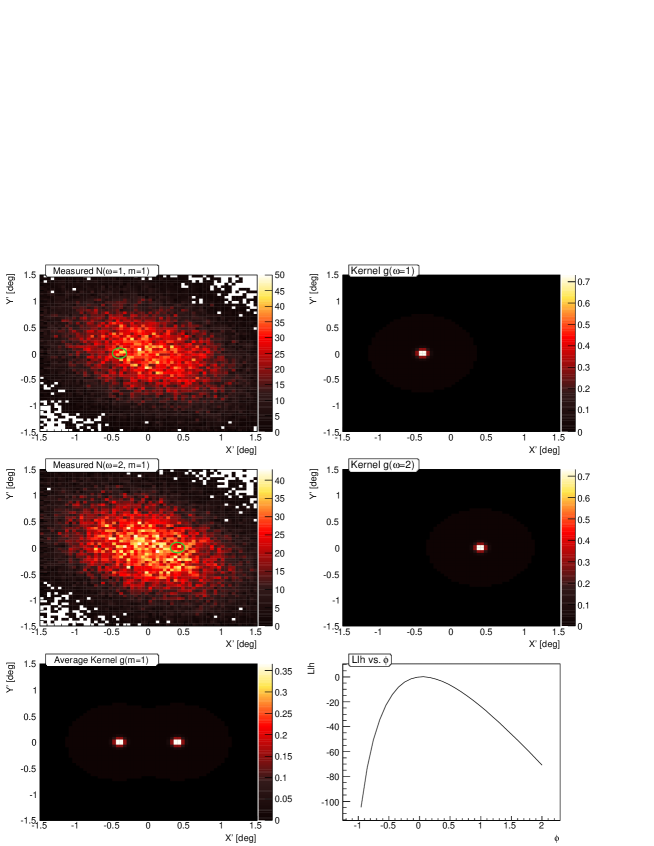
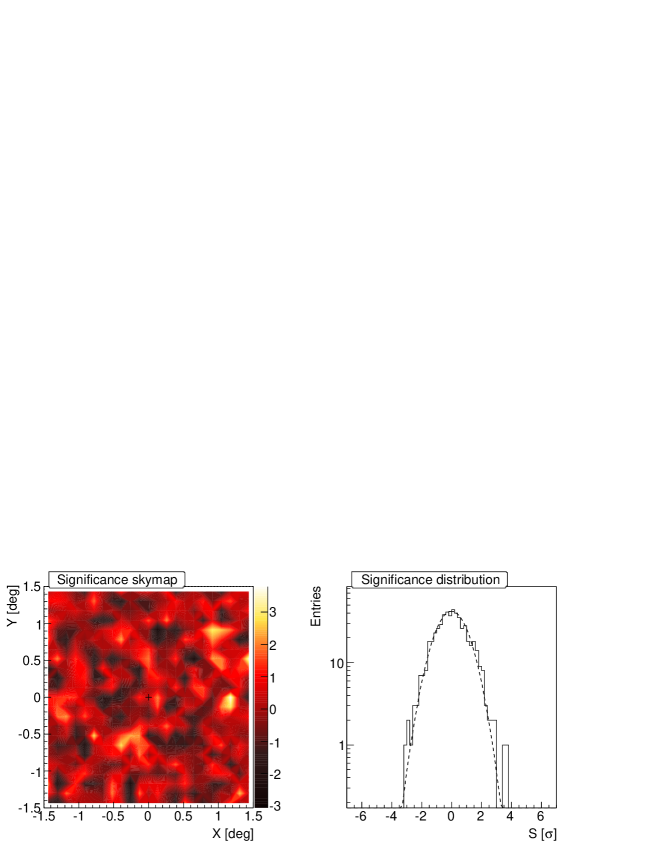
Figure 2: Case 1: W=2, M=1, asymmetric exposure shape, equal on-time, no source. In the upper left, the simulated measured distributions are shown, in coordinates relative to the observation center. Right of it are the kernels $g^{\omega}_{i}$, assuming the source to be at the observation center, and below is the corresponding average kernel $g^{m}_{i}$. The graph in the third row on the right is the log-likelihood as a function of $\phi$, and in the bottom row, the skymap and significance distribution are shown (the dotted line is a Gaussian of $\mu=0$ and $\sigma=1$). The observation center is marked with a cross in the sky map, and green circles in the data histograms.

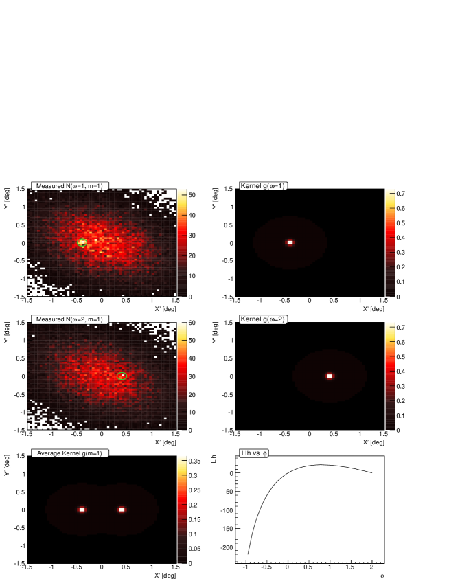
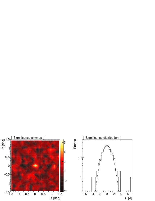
Figure 3: Same as Fig. 2, but with 300 excess events introduced at the observation center.

Figure 4: Same as Fig. 3, but with the detected excess included as an established source in the null hypothesis. The significance map is again consistent with the null hypothesis. Consequently, the log-likelihood function peaks at a relative excess parameter ($\phi$) that is significantly larger than zero.

5.2 Case 2: W=4, M=2, pointing-dependent exposure shape, very different exposure times, one additional off-data set, extended source with large offset

This is a very complex scenario that benchmarks the flexibility of the test statistic and the Likelihood Ratio Skymapping technique. The background events are distributed over 7 sub-histograms consisting of 3 wobble sets taken in two different operating conditions, and an additional set of off-data for one of the operating conditions. As can be seen in Fig. 5, the data can be combined without any problem, yielding an empty skymap and a Gaussian null-hypothesis distribution.

Figure 6 is the same scenario, but with 1200 photons added to mimic an extended source ($\sigma_{\mathrm{src}}=0.2^{\circ}$) at the large-offset sky coordinate $(0.4/1.0)$. Even using the same PSF-Kernel as before, the source can be detected ($5.5\,\mathrm{\sigma}$).

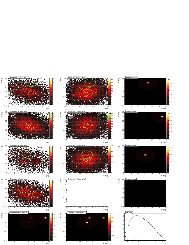
Figure 5: Case 2: W=4, M=2, pointing-dependent exposure shape, very different exposure times, one additional off-data set, The example kernel plots refer to the sky position $(0.4/1.0)$, marked with a cross in the significance skymap, where a source is injected in Fig. 6.

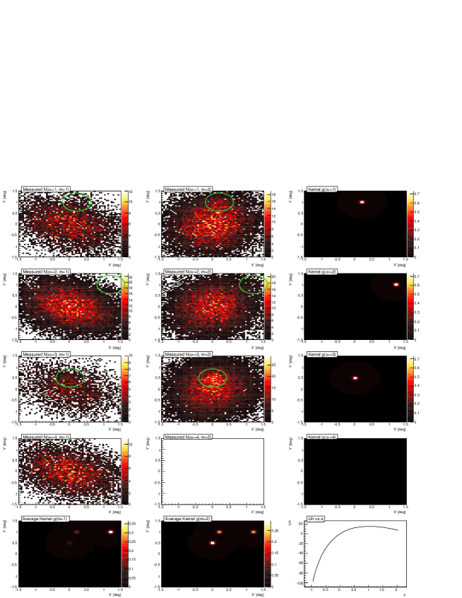
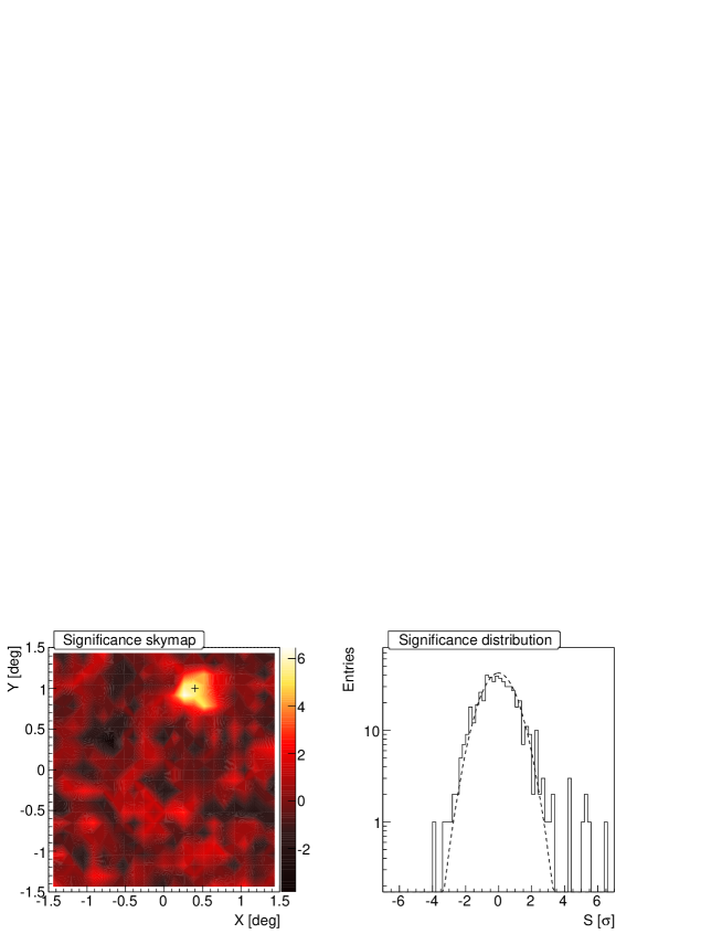
Figure 6: Same as Fig. 5, but with 1200 excess events introduced at the position marked with a green circle in the upper histograms.

5.3 Gaussian property of Eq. 16 and comparison to $S_{\mathrm{LM}}$

Figure 7 shows a simulation of significances calculated for the whole field of view of 20 signal-free skymaps simulated as in case 2 (Sec. 5.2). The distribution contains also bins of comparably small exposure and bins for which the optimization of the $\phi$-parameter reached its boundary condition. No treatment of the remaining correlation between the significances is undertaken. A Poissonian likelihood fit to the distribution yields Gaussian parameters of $\mu=-0.012\pm 0.010$ and $\sigma=1.006\pm 0.007$. The $\chi^{2}=40.5$ may be compared to the 37 non-zero bins of the distribution. This verifies both Eq. 16 as a Gaussian significance and the suggested recipes to deal with its features in the skymapping case.

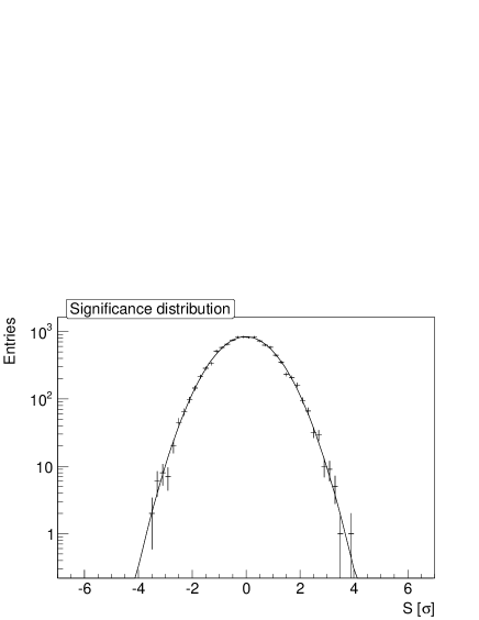
Figure 7: Accumulated significance distribution of 20 simulated skymaps as in Sec. 5.2. Despite the complex setup of several wobble positions and operating conditions, and the skymapping caveats outlined in Sec. 4.2.1, the significance distribution follows very well the shape of a Gaussian distribution (the solid line is the Gaussian fit to the data discussed in the text).

In the above case 1, the test statistic of Eq. 16 is somewhat higher than $S_{\mathrm{LM}}$, even though the latter involves an optimization of the applied integration radius (which is expected to lead to a selection bias). To study this possible trend systematically, Figure 8 shows the distribution of many significances obtained for the same case simulated 1000 times. It shows that while Eq. 16 does not always lead to a higher significance, there is a significant trend that in average it does.

Repeating this study with a lower background level, however, the effect is much weaker, while with a higher background density, the effect is stronger. This is assumably because with a low background density, the optimized $\theta^{2}$-cut will be large and include the whole signal, reducing the advantage of the known kernel from which Eq. 16 benefits.

The conclusion can be drawn that the test statistic presented in this work performs slightly better in cases with low signal-to-background ratios, and similar in cases where the dominant statistical uncertainty is that of the signal itself.

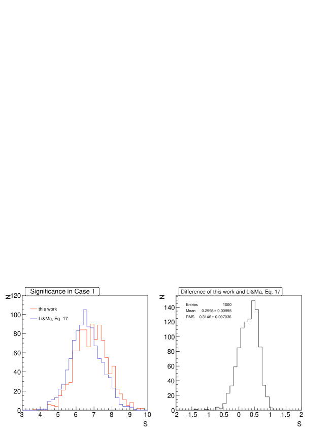
Figure 8: Comparison of significances obtained with Eq. 16 and $S_{\mathrm{LM}}$ (with optimized $\theta^{2}$-cut). Despite the trials implied by the optimized $\theta^{2}$-cut, Eq. 16 yields a systematically higher significance.

6 Conclusions

This paper derives a new generalized test statistic (Eq. 16) that can be used for significance calculation in VHE astronomy. The advantages over the existing test statistics are that it flexibly takes into account any number of data subsets from different wobble coordinates and operating conditions of the system, even if the acceptance shape is very irregular and different between these operating conditions. Also, it takes advantage of a known gamma-ray PSF while not requiring the optimization of an integration radius (”$\theta^{2}$-cut”).

The test statistic can be applied to any position in the field of view, so it is very suitable for skymapping purposes. The advantages of this approach is that the test statistic only makes minimal assumptions on the acceptance field of view and does not require any exposure symmetry or Monte Carlo simulations. It is hence unaffected by many systematic uncertainties. A ”Likelihood Ratio Skymapping” procedure is suggested in Sec. 4.2.

The log-likelihood function (Eq. 13) can also be applied to fit the shape and position parameters of the source. The formulae are furthermore extendable to accomodate established sources in the field of view, a non-homogeneous PSF shape or gamma-to-hadron acceptance ratio, an unbinned analysis approach or the ”orbit” observation mode. If the background event density is sufficiently high, the relative excess parameter $\phi$ is well-suited to calculate a gamma-ray flux map of the field of view.

In several simulated scenarios it is verified that the test statistic can not only handle the difficult situations it is designed for, but also seems to be systematically higher in the signal case, and therefore more sensitive, than the commonly used test statistic after Li and Ma [6], Eq. 17.

7 Acknowledgements

The author wishes to thank the MAGIC/CTA groups at IFAE, UAB and ICE for discussion of the results, and in particular Michele Doro, Daniel Mazin, Abelardo Moralejo, Takayuki Saito, Julian Sitarek and Victor Stamatescu for their useful comments on the draft. Also the support of the ”Juan de la Cierva” program of the Spanish MICINN is gratefully acknowledged.

References

- [1] CTA Consortium, Design Concepts for the Cherenkov Telescope Array. arXiv:1008.3703.
- [2] J. A. Hinton, et al., The status of the HESS project, New Astronomy Reviews 48 (2004) 331–337. arXiv:astro-ph/0403052, doi:10.1016/j.newar.2003.12.004.
- [3] J. Aleksić, et al., Performance of the MAGIC stereo system obtained with Crab Nebula data, accepted for publication in Astropart. Phys.arXiv:1108.1477.
- [4] J. Holder, et al., The first VERITAS telescope, Astroparticle Physics 25 (2006) 391–401. arXiv:astro-ph/0604119, doi:10.1016/j.astropartphys.2006.04.002.
- [5] D. Sobczynska, Natural limit on the /hadron separation for a stand alone air Cherenkov telescope, Journal of Physics G Nuclear Physics 34 (2007) 2279–2288. arXiv:astro-ph/0702562, doi:10.1088/0954-3899/34/11/005.
- [6] T.-P. Li, Y.-Q. Ma, Analysis methods for results in gamma-ray astronomy, ApJ 272 (1983) 317–324. doi:10.1086/161295.
- [7] V. P. Fomin, A. A. Stepanian, R. C. Lamb, D. A. Lewis, M. Punch, T. C. Weekes, New methods of atmospheric Cherenkov imaging for gamma-ray astronomy. I. The false source method, Astropart. Phys. 2 (1994) 137–150. doi:10.1016/0927-6505(94)90036-1.
- [8] F. Aharonian, et al., Evidence for TeV gamma ray emission from Cassiopeia A, A&A 370 (2001) 112–120. arXiv:astro-ph/0102391, doi:10.1051/0004-6361:20010243.
- [9] G. P. Rowell, A new template background estimate for source searching in TeV gamma -ray astronomy, A&A 410 (2003) 389–396. arXiv:astro-ph/0310025, doi:10.1051/0004-6361:20031194.
- [10] D. Berge, S. Funk, J. Hinton, Background modelling in very-high-energy -ray astronomy, A&A 466 (2007) 1219–1229. arXiv:astro-ph/0610959, doi:10.1051/0004-6361:20066674.
- [11] S. Lombardi, K. Berger, P. Colin, et al., Advanced stereoscopic gamma-ray shower analysis with the MAGIC telescopes, in: Proc. ICRC 2011 (arXiv:1109.6195), 2011.
-
[12]
S. S. Wilks, The
Large-Sample Distribution of the Likelihood Ratio for Testing Composite
Hypotheses, Ann. Math. Statist. 9 (1) (1938) 60–62.
URL http://projecteuclid.org/euclid.aoms/1177732360 - [13] W. Cash, Parameter estimation in astronomy through application of the likelihood ratio, ApJ 228 (1979) 939–947. doi:10.1086/156922.
- [14] J. A. Nousek, D. R. Shue, Chi-squared and C statistic minimization for low count per bin data, ApJ 342 (1989) 1207–1211. doi:10.1086/167676.
- [15] S. Gillessen, H. L. Harney, Significance in gamma-ray astronomy - the Li & Ma problem in Bayesian statistics, A&A 430 (2005) 355–362. arXiv:astro-ph/0411660, doi:10.1051/0004-6361:20035839.
- [16] R. Protassov, D. A. van Dyk, A. Connors, V. L. Kashyap, A. Siemiginowska, Statistics, Handle with Care: Detecting Multiple Model Components with the Likelihood Ratio Test, ApJ 571 (2002) 545–559. arXiv:astro-ph/0201547, doi:10.1086/339856.
- [17] S. N. Zhang, D. Ramsden, Statistical data analysis for gamma-ray astronomy, Experimental Astronomy 1 (1990) 145–163. doi:10.1007/BF00462037.
- [18] G. Finnegan, for the VERITAS Collaboration, Orbit Mode observation Technique Developed for VERITAS, Proc. Fermi Symposium 2011,arXiv:1111.0121.