Spectral Design of Dynamic Networks via Local Operations

Abstract

Motivated by the relationship between the eigenvalue spectrum of a network and the behavior of dynamical processes evolving in it, we propose a distributed iterative algorithm in which a group of $n$ autonomous agents self-organize the structure of their communication network in order to control the network’s eigenvalue spectrum. In our algorithm, we assume that each agent has only access to a local (‘myopic’) view of the network around it and that there is no centralized coordinator. In each iteration, agents of the network perform a decentralized decision process in which agents share limited information about their myopic vision of the network to find the most beneficial edge addition/deletion from a spectral point of view. We base our approach on a novel distance function defined in the space of eigenvalue spectra that is written in terms of the spectral moments of the Laplacian matrix. In each iteration, agents in the network run a greedy algorithm to find the edge addition/deletion that minimized the spectral distance to the desired spectrum. The spectral distance presents interesting theoretical properties that allow an elegant and efficient distributed implementation of the greedy algorithm using distributed consensus. Our distributed algorithm is stable by construction, i.e., locally optimizes the network’s eigenvalue spectrum, and is shown to perform very well in practice.

I Introduction

A wide variety of complex networks composed of autonomous agents are able to display a remarkable level of self-organization despite the absence of a centralized coordinator [1, 2]. For example, the intricate structure of many biological, social and economic networks, emerges as the result of local interactions between agents aiming to optimize their local utilities [3]. In most real cases, these agents have only access to myopic information about the structure of the network around them. Despite the limited information accessible to each agent, most of these “self-engineered” networks are able to efficiently satisfy their functional requirements.

The behavior of many networked dynamical processes, such as information spreading, synchronization, or decentralized coordination, is directly related to the network eigenvalue spectra [4]. In particular, the spectrum of the Laplacian matrix of a network plays a key role in the analysis of synchronization in networks of nonlinear oscillators [5, 6], as well as in the behavior of many distributed algorithms [7], and decentralized control problems [8, 9]. Motivated by the relationship between a network’s eigenvalue spectrum and the behavior of dynamical processes evolving in it, we propose a distributed iterative algorithm in which a group of autonomous agents self-organize the structure of their communication network in order to control the network’s eigenvalue spectrum. The evolution of the graph is ruled by a decentralized decision process in which agents share limited information about their myopic vision of the network to decide which network adjustment is most beneficial globally.

Optimization of network eigenvalues has been studied by several authors in both centralized [10, 11, 12] and decentralized settings [13]. In these papers, the objective is usually to find the weights associated to the edges of a given network in order to optimize eigenvalues of particular relevance, such as the Laplacian spectral gap or spectral radius (i.e., the second smallest and largest eigenvalues of the Laplacian matrix, respectively). In contrast to existing techniques, we propose a distributed framework where we control the so-called spectral moments of the Laplacian matrix by iteratively modifying the structure of the network. We show that the benefits of controlling the spectral moments, instead of individual eigenvalues, lies in lower computational cost and elegant distributed implementation. The performance of our algorithm is illustrated in nontrivial computer simulations.

The rest of this paper is organized as follows. In Section II, we review terminology and formulate the problem under consideration. In Section III, we introduce a decentralized algorithm to compute the spectral moments of the Laplacian matrix from myopic views of the network’s structure. We also introduce a novel perturbation technique to efficiently compute the effect of adding or removing edges on the spectral moments. Based on these results, in Section IV, we propose a distributed algorithm in which a group of autonomous agents modify their network of interconnections to control of the spectral moments of a network towards desired values. Finally, in Section V, we illustrate our approach with several computer simulations.

II Preliminaries & Problem Definition

II-A Eigenvalues of Graphs and their Spectral Moments

Let $\mathcal{G}=\left(\mathcal{V},\mathcal{E}\right)$ be an undirected graph, where $\mathcal{V}=\left\{1,\dots,n\right\}$ denotes a set of $n$ nodes and $\mathcal{E}\subseteq\mathcal{V}\times\mathcal{V}$ denotes a set of $e$ undirected edges. If $\left(i,j\right)\in\mathcal{E}$, we call nodes $i$ and $j$ adjacent (or first-neighbors), which we denote by $i\sim j$. We define the set of first-neighbors of a node $i$ as $\mathcal{N}_{i}=\{j\in\mathcal{V}:\left(i,j\right)\in\mathcal{E}\}.$ The degree $d_{i}$ of a vertex $i$ is the number of nodes adjacent to it, i.e., $d_{i}=\left|\mathcal{N}_{i}\right|$. An undirected graph is called simple if its edges are unweighted and it has no self-loops. A graph is weighted if there is a real number associated with every edge. More formally, a weighted graph $\mathcal{H}$ can be defined as the triad $\mathcal{H=}\left(\mathcal{V},\mathcal{E},\mathcal{W}\right)$, where $\mathcal{V}$ and $\mathcal{E}$ are the sets of nodes and edges in $\mathcal{H}$, and $\mathcal{W=}\left\{w_{ij}\in\mathbb{R},\text{ for all }\left(i,j\right)\in\mathcal{E}\right\}$ is the set of (possibly negative) weights.

Graphs can be algebraically represented via matrices. The adjacency matrix of a simple graph $\mathcal{G}$, denoted by $A_{\mathcal{G}}=[a_{ij}]$, is an $n\times n$ symmetric matrix defined entry-wise as $a_{ij}=1$ if nodes $i$ and $j$ are adjacent, and $a_{ij}=0$ otherwise. Given a weighted, undirected graph $\mathcal{H}$, the weighted adjacency matrix is defined by $W_{\mathcal{H}}=\left[w_{ij}\right]$, where $w_{ij}$ is the weight associated to edge $\left(i,j\right)\in\mathcal{E}$ and $w_{ij}=0$ if $i$ is not adjacent to $j$. We define the degree matrix of a simple graph $\mathcal{G}$ as the diagonal matrix $D_{\mathcal{G}}=diag\left(d_{i}\right)$. We define the Laplacian matrix $L_{\mathcal{G}}$ (also known as combinatorial Laplacian, or Kirchhoff matrix) of a simple graph as $L_{\mathcal{G}}=D_{\mathcal{G}}-A_{\mathcal{G}}$. For simple graphs, $L_{\mathcal{G}}$ is a symmetric, positive semidefinite matrix, which we denote by $L_{\mathcal{G}}\succeq 0$ [14]. Thus, $L_{\mathcal{G}}$ has a full set of $n$ real and orthogonal eigenvectors with real nonnegative eigenvalues $0=\lambda_{1}\leq\lambda_{2}\leq...\leq\lambda_{n}$. Furthermore, the trivial eigenvalue $\lambda_{1}=0$ of $L_{\mathcal{G}}$ always admits a corresponding eigenvector $v_{1}=\left(1,1,...,1\right)^{T}$. The algebraic multiplicity of the trivial eigenvalue is equal to the number of connected components in $\mathcal{G}$. The smallest and largest nontrivial eigenvalues of $L_{\mathcal{G}}$, $\lambda_{2}$ and $\lambda_{n}$, are called the spectral gap and spectral radius of $L_{\mathcal{G}}$, respectively.

Given an undirected (possibly weighted) graph $\mathcal{G}$, we denote its Laplacian spectrum by $S\left(\mathcal{G}\right)=\left\{\lambda_{1},...,\lambda_{n}\right\}$, and define the $k$-th Laplacian spectral moment of $\mathcal{G}$ as, [14]:

$$m_{k}\left(\mathcal{G}\right)\triangleq\frac{1}{n}\sum_{i=1}^{n}\lambda_{i}^{k}.$$ (1)

The following theorem states that an eigenvalue spectrum is uniquely characterized by a finite sequence of moments:

Theorem II.1

Consider two undirected (possibly weighted) graphs $G_{1}$ and $G_{2}$ with Laplacian eigenvalue spectra $S\left(G_{1}\right)=\{\lambda_{1}^{\left(1\right)}\leq...\leq\lambda_{n}^{\left(1\right)}\}$ and $S_{2}\left(G_{1}\right)=\{\lambda_{1}^{\left(2\right)}\leq...\leq\lambda_{n}^{\left(2\right)}\}$. Then, $\lambda_{i}^{\left(1\right)}=\lambda_{i}^{\left(2\right)}$ for all $1\leq i\leq n$ if and only if $m_{k}\left(G_{1}\right)=m_{k}\left(G_{2}\right)$ for $0\leq k\leq n-1$.

Proof:

In the Appendix.    

In the rest of this paper we will focus on the spectrum of the graph Laplacian matrix $L_{\mathcal{G}}$ and its spectral moments, which we denote by $m_{k}\left(L_{\mathcal{G}}\right)$. In this case, Theorem II.1, implies that the Laplacian spectral moment of a graph on $n$ nodes is uniquely characterize by the sequence of $n-1$ spectral moments $\left(m_{k}\left(L_{\mathcal{G}}\right)\right)_{k=1}^{n-1}$. It is worth remarking that two nonisomorphic graphs $\mathcal{G}_{1}$ and $\mathcal{G}_{2}$ can present the same eigenvalue spectrum [16], in which case we say that $\mathcal{G}_{1}$ and $\mathcal{G}_{2}$ are isospectral. In other words, the eigenvalue spectrum of a graph is not enough to characterize its structure. On the other hand, as we shall show in Section III, there are many interesting connections between the structural features of a graph $\mathcal{G}$ and the spectral moments of its Laplacian matrix, $m_{k}\left(L_{\mathcal{G}}\right)$.

II-B Local Structural Properties of Graphs

In this section we define a collection of structural properties that are important in our derivations. A walk of length $k$ from node $i_{1}$ to node $i_{k+1}$ is an ordered sequence of nodes $\left(i_{1},i_{2},...,i_{k+1}\right)$ such that $i_{j}\sim i_{j+1}$ for $j=1,2,...,k$. One says that the walk touches each of the nodes that comprises it. If $i_{1}=i_{k+1}$, then the walk is closed. A closed walk with no repeated nodes (with the exception of the first and last nodes) is called a cycle. Given a walk $p=\left(i_{1},i_{2},...,i_{k+1}\right)$ in a weighted graph $\mathcal{H}$ with weighted adjacency matrix $W_{\mathcal{H}}=\left[w_{ij}\right]$, we define the weight of the walk as, $\omega\left(p\right)=w_{i_{1}i_{2}}w_{i_{2}i_{3}}...w_{i_{k}i_{k+1}}$.

We now define the concept of local neighborhood around a node. Let $\delta\left(i,j\right)$ denote the distance between two nodes $i$ and $j$ (i.e., the minimum length of a walk from $i$ to $j$). By convention, we assume that $\delta\left(i,i\right)=0$. We define the $r$-th order neighborhood $\mathcal{G}_{i,r}=(\mathcal{N}_{i,r},\mathcal{E}_{i,r})$ around a node $i$ as the subgraph $\mathcal{G}_{i,r}\subseteq\mathcal{G}$ with node-set $\mathcal{N}_{i,r}\triangleq\left\{j\in\mathcal{V}:\delta\left(i,j\right)\leq r\right\}$, and edge-set $\mathcal{E}_{i,r}=\{(v,w)\in\mathcal{E}$ s.t. $v,w\in\mathcal{N}_{i,r}\}$. Given a set of $k$ nodes $\mathcal{K}\subseteq\mathcal{V}$, we define $\mathcal{G}_{\mathcal{K}}$ as the subgraph of $\mathcal{G}$ with node-set $\mathcal{V}\left(\mathcal{G}_{\mathcal{K}}\right)=\mathcal{K}$ and edge-set $\mathcal{E}\left(\mathcal{G}_{\mathcal{K}}\right)=\{\left(i,j\right)\in\mathcal{E}$ s.t. $i,j\in\mathcal{K}\}$. We define $L_{\mathcal{G}}\left(\mathcal{K}\right)$ as the $k\times k$ submatrix of $L_{\mathcal{G}}$ formed by selecting the rows and columns of $L_{\mathcal{G}}$ indexed by $\mathcal{K}$. In particular, we define the Laplacian submatrix $L_{i,r}\triangleq L_{\mathcal{G}}\left(\mathcal{N}_{i,r}\right)$.

We say that a structural measurement is local with a certain radius $r$ if it can be computed from the set of local neighborhoods $\{\mathcal{G}_{i,r}$, $i=1,...,n\}$. For example, the degree sequence of $\mathcal{G}$ is a local structural measurement (with radius $1$), since we can compute the degree of each node $i$ from the neighborhood $\mathcal{N}_{i,1}$. In contrast, the eigenvalue spectrum of the Laplacian matrix is not a local property, since we cannot compute the eigenvalues unless we know the complete graph structure. One of the main contributions of this paper is to propose a novel methodology to extract global information regarding the Laplacian eigenvalue spectrum from the set of local neighborhoods.

II-C Spectral Metrics and Problem Definition

As discussed in Section I, our goal is to propose a distributed algorithm to control the eigenvalue spectrum of a multi-agent network, via its spectral moments, by iteratively adding/removing edges in the network; see Section II-B. For this, we define the following spectral distance between two graphs $G_{a}$ and $G_{b}$, with spectra $S_{a}=\{\lambda_{i}^{\left(a\right)}\}_{i=1}^{n}$ and $S_{b}=\{\lambda_{i}^{\left(b\right)}\}_{i=1}^{n}$, as

$$d_{M}\left(S_{a},S_{b}\right)=\sum_{k=1}^{n-1}\left(m_{k}\left(G_{a}\right)^{1/k}-m_{k}\left(G_{b}\right)^{1/k}\right)^{2}.$$ (2)

According to Theorem II.1, two graphs are isospectral if their first $n-1$ spectral moments coincide; thus, $d_{M}$ in (2) is in fact a distance function in the space of graph spectra. We further define the spectral pseudometric:

$$d_{K}\left(S_{a},S_{b}\right)=\sum_{k=1}^{K}\left(m_{k}\left(G_{a}\right)^{1/k}-m_{k}\left(G_{b}\right)^{1/k}\right)^{2},$$ (3)

for $K<n-1$. The benefit of using the spectral pseudodistance versus other spectral distances is due to the fact that, as we shall show in Section III, we can efficiently compute the first $K$ spectral moments of the Laplacian matrix from the set of local Laplacian submatrices with radius $\left\lfloor K/2\right\rfloor$, i.e., $\{L_{i,\left\lfloor K/2\right\rfloor},i\in\mathcal{V}\}$. In other words, assuming that each agent has access to the Laplacian submatrix associated to its neighborhood with radius $r$, we shall show how to distributedly compute the first $2r+1$ Laplacian moments of the complete graph $L_{\mathcal{G}}$. With the notation defined above, we can rigorously state the problem addressed in this paper as follows:

Problem 1

Given a desired spectrum $S^{\ast}=\left\{\lambda_{i}^{\ast}\right\}_{i=1}^{n}$, find a simple graph $\mathcal{G}^{\ast}$ such that its Laplacian eigenvalue spectrum, denoted by $S\left(\mathcal{G}^{\ast}\right)$, minimizes $d_{K}\left(S\left(\mathcal{G}^{\ast}\right),S^{\ast}\right)$.

Finding a simple graph with a given (feasible ) eigenvalue spectrum is, in general, a hard combinatorial problem, even in a centralized setting. In this paper, we propose a distributed approximation algorithm to find a graph with a spectrum ‘close to’ $S^{\ast}$ in the $d_{K}$ pseudometric. In our algorithm, a group of agents located at the nodes of a network iteratively add/remove edges to drive the network’s eigenvalue spectrum towards the desired spectrum. In each iteration, the set of agents perform a decentralized decision process to find the most beneficial edge addition/deletion from the point of view of the global eigenvalue spectrum.

To formulate our algorithm, we first need to define the edit distance $d_{E}\left(\mathcal{G}_{a},\mathcal{G}_{b}\right)$ between two graphs $\mathcal{G}_{a}$ and $\mathcal{G}_{b}$, which is the minimum number of edge additions plus edge deletions to transform $\mathcal{G}_{a}$ into a graph that is isomorphic to $\mathcal{G}_{b}$. To approximately solve Problem 1 in a distributed way, we propose the following iteration to determine a sequence of graphs $\{\mathcal{G}(t)\}_{t\geq 0}$, starting from any graph $\mathcal{G}_{0}$:

$$\mathcal{G}(t+1)\triangleq$$

s.t.

(4)

The resulting sequence of spectra $\{S\left(\mathcal{G}(t)\right)\}_{t\geq 0}$ converges to $S^{\ast}$ as $t$ grows. The constraint $d_{E}\left(\mathcal{G}\left(t\right),\mathcal{G}\left(t+1\right)\right)=1$ enforces only single edge additions or deletions at each iteration, while the requirement $\lambda_{2}\left(\mathcal{G}\left(t\right)\right)>0$ enforces graph connectivity at all times, which will be necessary for the distributed implementation in Section IV. Note that the Iteration (4) typically requires global knowledge of the network structure. In this paper, we propose a computationally efficient, distributed algorithm in which agents in the network solve (4) using only their local, myopic views of the network structure. In particular, we shall show how the set of agents can compute, in a distributed fashion, the effect of an edge addition/deletion on the first $2r+1$ Laplacian moments. Furthermore, we shall also propose a distributed algorithm to find the edge addition/deletion that minimizes the resulting value of the spectral pseudodistance to $S^{\ast}$. Before we describe the implementation details in Section IV, we first provide the theoretical foundation for our approach in Section III.

Remark II.1 (Convergence)

Several remarks are in order. First, note that it is not always possible to find a simple graph that exactly match a given eigenvalue spectrum. Second, the spectral pseudometric $d_{K}\left(S\left(\mathcal{G}\right),S^{\ast}\right)$ may present multiple minima for a given $S^{\ast}$. These minima could correspond, for example, to several isospectral graphs matching the desired spectrum $S^{\ast}$ [16]. Therefore, iteration (4) may converge to different isospectral graphs depending on the initial condition $\mathcal{G}_{0}$. Third, iteration (4) finds the most beneficial edge addition/deletion in each time step, hence, this greedy approach may get trapped in a local minimum. In practice, we observe that in our numerical simulations the spectra of these local minima are remarkably close to those of the desired spectrum.

III Moment-Based Analysis of the Laplacian Matrix

In this section, we use tools from algebraic graph theory to compute the spectral moments of the Laplacian matrix of $\mathcal{G}$ when only the set of local Laplacian submatrices $\left\{L_{i,r}\text{, }i\in\mathcal{V}\right\}$ is available. As a result of our analysis, we propose a decentralized algorithm to compute a truncated sequence of Laplacian spectral moments via a single distributed averaging. Furthermore, we also present an efficient approach to compute the effect of adding or deleting an edge in the Laplacian spectral moments of the graph. Particularly useful in our derivations will be the following result from algebraic graph theory [14]:

Lemma III.1

Let $\mathcal{H=}\left(\mathcal{V},\mathcal{E},\mathcal{W}\right)$ be a weighted graph with weighted adjacency matrix $W_{\mathcal{H}}=\left[w_{ij}\right]$. Then

$$\left[W_{\mathcal{H}}^{k}\right]_{ii}=\sum_{p\in P_{i,k}\left(\mathcal{H}\right)}\omega\left(p\right),$$

where $P_{i,k}\left(\mathcal{H}\right)$ is the set of closed walks of length $k$ starting and finishing at node $i$ in the weighted graph $\mathcal{H}$.

III-A Algebraic Analysis of Structured Matrices

Consider the symmetric Laplacian matrix $L_{\mathcal{G}}$ of a simple graph $\mathcal{G=}\left(\mathcal{V},\mathcal{E}\right)$. We denote by $\mathcal{G}_{i,r}=\left(\mathcal{N}_{i,r},\mathcal{E}_{i,r}\right)$ the neighborhood of radius $r$ around node $i$ and define the local Laplacian submatrix $L_{i,r}$, as the submatrix $L_{\mathcal{G}}\left(\mathcal{N}_{i,r}\right)$, formed by selecting the rows and columns of $L_{\mathcal{G}}$ indexed by the set of nodes $\mathcal{N}_{i,r}$. By convention, we associate the first row and column of the submatrix $L_{i,r}$ with node $i\in\mathcal{V}$, which can be done via a simple permutation of rows and columns. For a simple graph $\mathcal{G}$ with Laplacian matrix $L_{\mathcal{G}}$, we define $\mathcal{L}\left(\mathcal{G}\right)$ as the weighted graph whose adjacency matrix is equal to $L_{\mathcal{G}}$. In other words, $\mathcal{L}\left(\mathcal{G}\right)$ has edges with weight $-1$ for $\left(i,j\right)\in\mathcal{E}\left(\mathcal{G}\right)$, $0$ for $\left(i,j\right)\not\in\mathcal{E}\left(\mathcal{G}\right)$, and $d_{i}$ for all self-loops $\left(i,i\right)$, $i\in\mathcal{V}\left(\mathcal{G}\right)$. We also define $\mathcal{H}_{i,r}$ as the weighted subgraph of $\mathcal{L}\left(\mathcal{G}\right)$ with node set $\mathcal{N}_{i,r}$, containing all the edges of $\mathcal{L}\left(\mathcal{G}\right)$ connecting pairs of nodes in $\mathcal{N}_{i,r}$ (including self-loops). Notice that, according to this definition, the weighted adjacency matrix of $\mathcal{H}_{i,r}$ is equal to $L_{i,r}$.

In this paper, we assume that each agent in the network knows the structure of its local neighborhood $\mathcal{G}_{i,r}$, for a fixed $r$. Therefore, agent $i$ has access to the local Laplacian submatrix $L_{i,r}$. The following results allows us aggregate information from the set of local Laplacian submatrices, $\left\{L_{i,r}\right\}_{i\in\mathcal{V}}$, to compute a sequence of spectral moments of the (global) Laplacian matrix $L_{\mathcal{G}}$.

Theorem III.2

Consider a simple graph $\mathcal{G}$ with Laplacian matrix $L_{\mathcal{G}}$. Then, for a given radius $r$, the Laplacian spectral moments can be written as

$$m_{k}\left(L_{\mathcal{G}}\right)=\frac{1}{n}\sum_{i=1}^{n}\left[L_{i,r}^{k}\right]_{11},$$ (5)

for $k\leq K=2r+1$.

Proof:

Since the trace of a matrix is the sum of its eigenvalues, we can expand the $k$-th spectral moment of the Laplacian matrix as follows:

$$m_{k}\left(L_{\mathcal{G}}\right) = \frac{1}{n}\text{Trace}\left(L_{\mathcal{G}}^{k}\right)$$

$$= \frac{1}{n}\sum_{i=1}^{n}\left[L_{\mathcal{G}}^{k}\right]_{ii}$$

Therefore, since $L_{\mathcal{G}}$ is the weighted adjacency matrix of the Laplacian graph $\mathcal{L}\left(\mathcal{G}\right)$, we have (from Lemma III.1)

$$m_{k}\left(L_{\mathcal{G}}\right)=\frac{1}{n}\sum_{i=1}^{n}\sum_{p\in P_{i,k}\left(\mathcal{L}\left(\mathcal{G}\right)\right)}\omega\left(p\right),$$ (6)

where the weights $\omega\left(p\right)$ are summed over the set of closed walks of length $k$ starting at node $i$ in the weighted graph $\mathcal{L}\left(\mathcal{G}\right)$.

For a fixed value of $k$, closed walks of length $k$ in $\mathcal{L}\left(\mathcal{G}\right)$ starting at node $i$ can only touch nodes within a certain distance $r\left(k\right)$ of $i$, where $r\left(k\right)$ is a function of $k$ (see Fig. 1). In particular, for $k$ even (resp. odd), a closed walk of length $k$ starting at node $i$ can only touch nodes at most $k/2$  (resp. $\left\lfloor k/2\right\rfloor$) hops away from $i$. Therefore, closed walks of length $k$ starting at $i$ are always contained within the neighborhood of radius $\left\lfloor k/2\right\rfloor$. In other words, the neighborhood $\mathcal{G}_{i,r}$ of radius $r$ contains all closed walks of length up to $2r+1$ starting at node $i$. Therefore, for $k\leq 2r+1$, we have that

$$\sum_{p\in P_{i,k}\left(\mathcal{L}\right)}\omega\left(p\right)=\sum_{p\in P_{1,k}\left(\mathcal{H}_{i,r}\right)}\omega\left(p\right),$$

where $\mathcal{H}_{i,r}$ is the weighted graph whose adjacency matrix is equal to the local Laplacian submatrix $L_{i,r}$ (notice that, by convention, we associate the first row and column of $L_{i,r}$ with node $i$). Therefore, according to Lemma III.1, we have

$$\sum_{p\in P_{1,k}\left(\mathcal{H}\left(L_{i,r}\right)\right)}\omega\left(p\right)=\left[L_{i,r}^{k}\right]_{1,1}.$$ (7)

Then, substituting (7) into (6), we obtain the statement of our Theorem.    

Remark III.1 (Distributed computation of spectral moments)

Since every node $i$ has access to its local neighborhood $\mathcal{G}_{i,r}$, it is possible to compute the first $2r+1$ moments via a simple distributed averaging of the quantities $\{\left[L_{i,r}^{k}\right]_{1,1}\}_{i\in\mathcal{V}}$, [7]. This averaging efficiently aggregates local pieces of local structural information (described by the local Laplacian submatrices) to produce a truncated sequence of spectral moments of the (global) Laplacian matrix. This is an useful result for the analysis of complex networks for which retrieving the complete structure of the network can be very challenging (in many cases, not even possible).

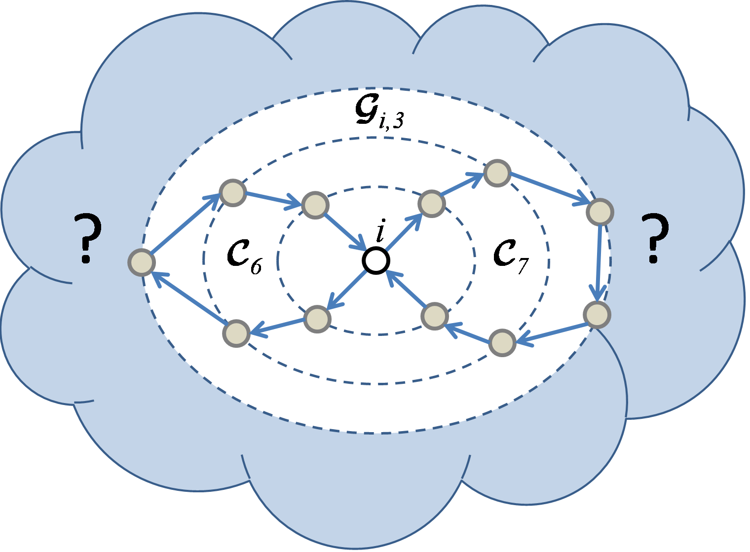
Figure 1: Cycles $\mathcal{C}_{6}$ and $\mathcal{C}_{7}$, of lengths $6$ and $7\,$, in a neighborhood of radius $3$ around node  $i\,$.

Based on Theorem III.2, we propose a distributed algorithm to compute a sequence of $2r+1$ spectral moments of $L_{\mathcal{G}}$ from local submatrices $L_{i,r}$, as described in Algorithm 1. Note that, computing the spectral moments via (5) is much more efficient than computing these moments via an explicit eigenvalue decomposition for many real-world networks. In most real applications, the Laplacian matrix representing the network structure is a sparse graph for which the number of nodes in the neighborhood $\mathcal{N}_{i,r}$ is very small compared to $n$, for moderate values of $r$.

Algorithm 1 Decentralized moment computation

0:  Local Laplacian submatrices $L_{i,r}$ for all nodes $i\in V$;

1:  Each node $i\in V$ computes a vector $\mathbf{\mu}_{i}\triangleq\left(\mu_{i,1},\mu_{i,2},\mu_{i,3},...,\mu_{i,2r+1}\right)^{T}$, where $\mu_{i,k}\triangleq\left[L_{i,r}^{k}\right]_{1,1}$;

2:  Using distributed averaging, compute the following vector of averages:

$$\mathbf{m}_{2r+1}\left(L_{\mathcal{G}}\right) \triangleq \frac{1}{n}\sum_{i=1}^{n}\mathbf{\mu}_{i}$$

$$= \frac{1}{n}\sum_{i=1}^{n}\left(0,\mu_{i,2},\mu_{i,3},...,\mu_{i,2r+1}\right)^{T}$$

$$= \left(m_{1}\left(L_{\mathcal{G}}\right),m_{2}\left(L_{\mathcal{G}}\right),...,m_{2r+1}\left(L_{\mathcal{G}}\right)\right)^{T}.$$

III-B Moment-Based Perturbation Analysis

In this section, we use spectral graph theory to compute the effect of adding or deleting an edge on the spectral moments of the Laplacian matrix. Traditionally, the effect of a matrix perturbation on the eigenvalue spectrum is analyzed using eigenvalue perturbation techniques [17]. In particular, the effect of adding a ‘small’ perturbation matrix $\delta W$ to an $n\times n$ symmetric matrix $W$ with eigenvalue spectrum $\left\{\sigma_{k}\right\}_{k=1}^{n}$ can be approximated, in the first-order, by [17]

$$\widetilde{\sigma}_{k}-\sigma_{k}\approx u_{k}^{T}~{}\delta W~{}u_{k},$$

where $u_{k}$ is the eigenvector of $W$ associated with the eigenvalue $\sigma_{k}$, and $\left\{\widetilde{\sigma}_{k}\right\}_{k=1}^{n}$ is the eigenvalue spectrum of the perturbed matrix $W+\delta W$. In the case of the Laplacian matrix, the perturbation matrix $\delta W$ corresponding to the addition of an edge $\left(i,j\right)$ can be written as, $\delta W=\left(e_{i}-e_{j}\right)\left(e_{i}-e_{j}\right)^{T}$, where $e_{i}$ is the unit vector in the direction of the $i$-th coordinate. We denote by $\mathcal{G}+\left(i,j\right)$ the graph resulting of adding edge $\left(i,j\right)$ to $\mathcal{G}$, and $\{\widetilde{\lambda}_{k}\}_{k=1}^{n}$ is the Laplacian spectrum of $\mathcal{G}+\left(i,j\right)$. Therefore, adding edge $\left(i,j\right)$ perturbs the eigenvalues of the Laplacian matrix as follows:

$$\widetilde{\lambda}_{k}-\lambda_{k} \approx v_{k}^{T}\left(e_{i}-e_{j}\right)\left(e_{i}-e_{j}\right)^{T}v_{k}$$

$$= \left(v_{k,i}-v_{k,j}\right)^{2},$$

where $v_{k}$ is the eigenvector of $L_{\mathcal{G}}$ associated to $\lambda_{k}$, and $v_{k,j}$ is its $j$-th component. Hence, the resulting spectral radius can be approximated as

$$\widetilde{\lambda}_{1}\approx\lambda_{1}+\left(v_{1,i}-v_{1,j}\right)^{2}.$$

Therefore, computing the effect of an edge addition on the spectral radius using traditional perturbation techniques requires computation of the dominant eigenvalue and eigenvector of $L_{\mathcal{G}}$, which is computationally expensive for very large graphs. As an alternative to the traditional analysis, we propose a novel approach, based on algebraic graph theory, to compute the effect of structural perturbation on the spectral moments of the Laplacian matrix $L_{\mathcal{G}}$ without explicitly computing the eigenvalues or eigenvectors of $L_{\mathcal{G}}$. Furthermore, our approach can be efficiently implemented in a fully decentralized manner.

In our derivations, we use the following result from algebraic graph theory:

Lemma III.3

Let $\mathcal{H=}\left(\mathcal{V},\mathcal{E},\mathcal{W}\right)$ be a weighted graph with weighted adjacency matrix $W_{\mathcal{H}}=\left[w_{ij}\right]$. Then

$$m_{k}\left(W_{\mathcal{H}}\right)=\frac{1}{n}\sum_{p\in P_{k}\left(\mathcal{H}\right)}\omega\left(p\right),$$ (8)

where $P_{k}\left(\mathcal{H}\right)$ is the set of closed walks of length $k$ in the weighted graph $\mathcal{H}$.

Proof:

This lemma is a consequence of Lemma III.1. Specifically, we have that

$$m_{k}\left(W\left(\mathcal{H}\right)\right) = \frac{1}{n}\text{Trace}\left(W\left(\mathcal{H}\right)^{k}\right)$$

$$= \frac{1}{n}\sum_{i\in\mathcal{V}}\left[W\left(\mathcal{H}\right)^{k}\right]_{i,i}$$

$$= \frac{1}{n}\sum_{i\in\mathcal{V}}\sum_{p\in P_{i,k}\left(\mathcal{H}\right)}\omega\left(p\right)$$

$$= \frac{1}{n}\sum_{p\in P_{k}\left(\mathcal{H}\right)}\omega\left(p\right),$$

where $P_{k}\left(\mathcal{H}\right)\triangleq\cup_{i\in\mathcal{V}}P_{i,k}\left(\mathcal{H}\right)$ is the set of all closed walks of length $k$ in $\mathcal{H}$ (for any starting node $i\in\mathcal{V}$).    

III-C Perturbation on the Spectral Moments

Consider a simple graph $\mathcal{G}$ with Laplacian matrix $L_{\mathcal{G}}$. We denote by $\mathcal{G}+\left(i,j\right)$ (resp. $\mathcal{G}-\left(i,j\right)$) the graph resulting from adding (resp. removing) edge $\left(i,j\right)$ to (resp. from) $\mathcal{G}$. Consider the sets of nodes $\mathcal{N}_{i,r}$ and $\mathcal{N}_{j,r}$ being within a radius $r$ from node $i$ and node $j$, respectively. Let us define the following submatrices indexed by the set of nodes in $\mathcal{N}_{i,r}\cup\mathcal{N}_{j,r}$:

$$U_{r,\left(i,j\right)} \triangleq L_{\mathcal{G}}\left(\mathcal{N}_{i,r}\cup\mathcal{N}_{j,r}\right),$$

$$U_{r,\left(i,j\right)}^{+} \triangleq L_{\mathcal{G}+\left(i,j\right)}\left(\mathcal{N}_{i,r}\cup\mathcal{N}_{j,r}\right),$$

$$U_{r,\left(i,j\right)}^{-} \triangleq L_{\mathcal{G}-\left(i,j\right)}\left(\mathcal{N}_{i,r}\cup\mathcal{N}_{j,r}\right).$$

The following lemma allows us to efficiently compute the increment (resp. decrement) in the Laplacian spectral moments of $\mathcal{G}$ due to the addition (resp. removal) of edge $\left(i,j\right)$:

Theorem III.4

Given a simple graph $\mathcal{G}$ with Laplacian matrix $L_{\mathcal{G}}$, the increment (decrement) in the $k$-th Laplacian spectral moment of a graph $\mathcal{G}$ due to the addition or deletion of an edge $\left(i,j\right)$ can be written as

$$m_{k}\left(L_{\mathcal{G}\pm\left(i,j\right)}\right)-m_{k}\left(L_{\mathcal{G}}\right)=\frac{1}{n}\left(\text{Trace}\left(U_{r,\left(i,j\right)}^{\pm}\right)^{k}-\text{Trace}\left(U_{r,\left(i,j\right)}\right)^{k}\right),$$ (9)

for $k\leq 2r+1$.

Proof:

Consider the weighted Laplacian graphs of $L_{\mathcal{G}}$, $L_{\mathcal{G}+\left(i,j\right)}$, and $L_{\mathcal{G}-\left(i,j\right)}$, which we denote by $\mathcal{H}\triangleq\mathcal{L}\left(\mathcal{G}\right)$, $\mathcal{H}^{+}\triangleq\mathcal{L}\left(\mathcal{G}+\left(i,j\right)\right)$ and $\mathcal{H}^{-}\triangleq\mathcal{L}\left(\mathcal{G}-\left(i,j\right)\right)$, respectively. (By definition, the adjacency matrices of the Laplacian graphs are the Laplacian matrices of the graphs.) Then, according to Lemma III.3, we have that the $k$-th spectral moments $m_{k}\left(L_{\mathcal{G}}\right)$, $m_{k}\left(L_{\mathcal{G}+\left(i,j\right)}\right)$ and $m_{k}\left(L_{\mathcal{G}-\left(i,j\right)}\right)$ can be written as weighted sums over the sets of all closed walks of length $k$ in $\mathcal{H}$, $\mathcal{H}^{+}$, and $\mathcal{H}^{-}$, as follows,

$$m_{k}\left(L_{\mathcal{G}}\right) = \frac{1}{n}\sum_{p\in P_{k}\left(\mathcal{H}\right)}\omega\left(p\right),$$

$$m_{k}\left(L_{\mathcal{G}\pm\left(i,j\right)}\right) = \frac{1}{n}\sum_{p\in P_{k}\left(\mathcal{H}^{\pm}\right)}\omega\left(p\right).$$

We define $P_{k,r}^{\left(i,j\right)}\left(\mathcal{H}\right)$, $P_{k,r}^{\left(i,j\right)}\left(\mathcal{H}^{+}\right)$, and $P_{k,r}^{\left(i,j\right)}\left(\mathcal{H}^{-}\right)$ as the sets of closed walks of length $k$ in, respectively, $\mathcal{H}$, $\mathcal{H}^{+}$, and $\mathcal{H}^{-}$ visiting only nodes in the set $\mathcal{N}_{i,r}\cup\mathcal{N}_{j,r}$. Then, we can split the summation in (8) for the Laplacian matrices, as follows:

$$m_{k}\left(L_{\mathcal{G}}\right) = \frac{1}{n}\sum_{p\in P_{k,r}^{\left(i,j\right)}\left(\mathcal{H}\right)}\omega\left(p\right)+\frac{1}{n}\sum_{p\in P_{k}\backslash P_{k,r}^{\left(i,j\right)}\left(\mathcal{H}\right)}\omega\left(p\right),$$ (10)

$$m_{k}\left(L_{\mathcal{G}\pm\left(i,j\right)}\right) = \frac{1}{n}\sum_{p\in P_{k,r}^{\left(i,j\right)}\left(\mathcal{H}^{\pm}\right)}\omega\left(p\right)+\frac{1}{n}\sum_{p\in P_{k}\backslash P_{k,r}^{\left(i,j\right)}\left(\mathcal{H}^{\pm}\right)}\omega\left(p\right).$$ (11)

Notice that, as we illustrated in Fig. 1, none of the closed walk of length $k\leq 2r+1$ touching node $i$ (resp. node $j$) can leave the neighborhood $\mathcal{N}_{i,r}$ (resp. $\mathcal{N}_{j,r}$). Therefore, all closed walks of length $k\leq 2r+1$ touching either node $i$ or $j$ (or both) are contained in $\mathcal{N}_{i,r}\cup\mathcal{N}_{j,r}$. As a consequence, none of the closed walks in $P_{k}\backslash P_{k}^{\left(i,j\right)}\left(\mathcal{H}\right)$ or $P_{k}\backslash P_{k}^{\left(i,j\right)}\left(\mathcal{H}^{\pm}\right)$ touches node $i$ or $j$. Since addition/removal of edge $\left(i,j\right)$ does not influence those walks not touching $i$ or $j$, we have that

$$\sum_{p\in P_{k}\backslash P_{k,r}^{\left(i,j\right)}\left(\mathcal{H}\right)}\omega\left(p\right)=\frac{1}{n}\sum_{p\in P_{k}\backslash P_{k,r}^{\left(i,j\right)}\left(\mathcal{H}^{\pm}\right)}\omega\left(p\right).$$

Thus, from (10) and (11) we have

$$m_{k}\left(L_{\mathcal{G}^{\pm}\left(i,j\right)}\right)-m_{k}\left(L_{\mathcal{G}}\right)=\frac{1}{n}\sum_{p\in P_{k,r}^{\left(i,j\right)}\left(\mathcal{H}^{{}^{\pm}}\right)}\omega\left(p\right)-\frac{1}{n}\sum_{p\in P_{k,r}^{\left(i,j\right)}\left(\mathcal{H}\right)}\omega\left(p\right).$$ (12)

Since $P_{k,r}^{\left(i,j\right)}\left(\mathcal{H}\right)$ is the set of all closed walks of length $k$ in $\mathcal{H}$ visiting nodes in the set $\mathcal{N}_{i,r}\cup\mathcal{N}_{j,r}$, we can apply Lemma III.3 to obtain

$$\frac{1}{n}\sum_{p\in P_{k,r}^{\left(i,j\right)}\left(\mathcal{H}\right)}\omega\left(p\right) = m_{k}\left(L_{\mathcal{G}}\left(\mathcal{N}_{i,r}\cup\mathcal{N}_{j,r}\right)\right)$$ (13)

$$= \frac{1}{n}\text{Trace}\left(U_{r,\left(i,j\right)}\right)^{k}.$$

Similarly, for $P_{k,r}^{\left(i,j\right)}\left(\mathcal{H}^{{}^{\pm}}\right)$, we obtain

$$\frac{1}{n}\sum_{p\in P_{k,r}^{\left(i,j\right)}\left(\mathcal{H}^{{}^{\pm}}\right)}\omega\left(p\right)=\frac{1}{n}\text{Trace}\left(U_{r,\left(i,j\right)}^{\pm}\right)^{k}.$$ (14)

Finally, substituting (13) and (14) in (12) provides us with the statement of our theorem.    

Remark III.2 (Computational cost)

According to Lemma III.4, we can compute the increment or decrement in the Laplacian spectral moments (up to order $2r+1$) by computing Trace$(U_{r,\left(i,j\right)})^{k}$ and Trace$(U_{r,\left(i,j\right)}^{\pm})^{k}$. Notice that the sizes of $U_{r,\left(i,j\right)}$ and $U_{r,\left(i,j\right)}^{\pm}$ are $\left|\mathcal{N}_{i,r}\cup\mathcal{N}_{j,r}\right|$, which is usually small for large sparse graphs (and moderate $r$).

IV Decentralized Control of Spectral Moments

In this section, we integrate the results developed in Section III with a novel technique for distributed connectivity verification of edge additions or deletions in order to obtain a distributed solution to Problem 1 in the form of (4), as discussed in Section II-C. This relies on the assumption that an agent at node $i$ is able to communicate at time slot $t$ with all the agents in its first-order neighborhood $\mathcal{N}_{i,1}\left(t\right)$ only. Moreover, we also assume that every agent has only a myopic view of the network structure. This means that at time slot $t$ agent $i\in\mathcal{V}$ only knows the topology of the neighborhood $\mathcal{G}_{i,r}\left(t\right)$, within a particular radius $r$. This limits the set of possible actions that every agent $i$ can take in every step of the iteration (4), to be local edge additions of non-edges $\left(i,j\right)\not\in\mathcal{E}\left(t\right)$ in $\mathcal{G}_{i,r}\left(t\right)$ or local edge deletions of edges $\left(i,j\right)\not\in\mathcal{E}\left(t\right)$ in $\mathcal{G}_{i,1}\left(t\right)$.

In what follows, it will be useful to predetermine the master node for each edge $\left(i,j\right)\in\mathcal{E}\left(t\right)$, which can be arbitrarily chosen from the set of nodes $\left\{i,j\right\}$. The notion of master node is useful to coordinate actions in our decentralized algorithm. The agent located at the master node of $\left(i,j\right)$ is the only one with the authority to decide if edge $\left(i,j\right)$ is deleted. We denote by $\mathcal{D}_{i}(t)$ the set of edges having node $i$ as its master. In our simulations, we choose this set to be $\mathcal{D}_{i}(t)\triangleq\left\{\left(i,j\right)\in\mathcal{E}(t)\;|\;i>j\right\}$. Similarly, it is useful to predefine a master node for each nonedge $\left(i,k\right)\not\in\mathcal{E}\left(t\right)$. The agent located at the master node of the nonedge is the only one with the authority to decide if edge $\left(i,k\right)$ is added to the network. We denote by $\mathcal{A}_{i}\left(t\right)$ the set of nonedges having node $i$ as its master. In our case, we define this set as $\mathcal{A}_{i}\left(t\right)\triangleq\left\{\left(i,k\right)\not\in\mathcal{E}(t)\;|\;k\in\mathcal{N}_{i,r}(t)\text{ and}\;i>k\right\}$, where we limit node $k$ to be in $\mathcal{N}_{i,r}(t)$, since we are only considering local edge additions.

IV-A Connectivity-Preserving Edge Deletions

In a centralized framework, network connectivity can be inferred from the number of trivial eigenvalues of the Laplacian matrix. However, when only local network information is available, only sufficient conditions for connectivity can be verified. One such condition is the requirement that $\left|\mathcal{N}_{j}\left(t\right)\cap\mathcal{N}_{i,r}\left(t\right)\right|>1$, which can be locally verified by agent $i$ with knowledge of only $\mathcal{G}_{i,r}$. Since this condition is only sufficient but not necessary for connectivity preservation, we need a mechanism to check connectivity for those edges in the set

$$\mathcal{C}\left(t\right)=\left\{\left(i,j\right)\in\mathcal{E}(t)\;:\;\left|\mathcal{N}_{j}\left(t\right)\cap\mathcal{N}_{i,r}\left(t\right)\right|=1\right\}.$$

of critically connected edges, for which the sufficient condition does not hold.

The proposed mechanism relies on a the concept of a maximum consensus. In particular, consider a graph $\mathcal{G}(t)=\left(\mathcal{V},\mathcal{E}(t)\right)$ at time $t\geq 0$ and for any $(i,j)\in\mathcal{C}(t)$ associate a scalar variable $x_{k}^{(i,j)}(s)\in\mathbb{R}$ with every node $k\in\mathcal{V}$. Assume that the variables $x_{k}^{(i,j)}(s)$ are randomly initialized and run the following maximum consensus update

$$x_{k}^{(i,j)}\left(s+1\right)=\max_{l\in\mathcal{N}_{k,1}-\{i,j\}}\{x_{l}^{(i,j)}\left(s\right)\}$$ (15)

on the graph $\mathcal{G}(t)-(i,j)$ obtained by virtually disabling the link $(i,j)$ via blocking communication through it. Then, the network $\mathcal{G}(t)-(i,j)$ is almost surely connected if and only if the variables $x_{k}^{(i,j)}(s)$ for all $k\in\mathcal{V}$ converge to the common value $\max_{k}x_{k}^{(i,j)}\left(0\right)$. Note that convergence in this case takes place in finite time that is upper bounded by the diameter of the network [18]. This idea can be extended to simultaneous verification of multiple link deletions in $\mathcal{C}\left(t\right)$. In fact, since every edge is assigned a unique master agent, we can partition the set $\mathcal{C}(t)$ in to $|\mathcal{V}|$ disjoint subsets $\mathcal{C}(t)\cap\mathcal{D}_{i}(t)$ for all $i\in\mathcal{V}$. This allows us to define the sets $\mathcal{P}_{ki}=\{x_{k}^{\left(i,j\right)}\left(s\right):\left(i,j\right)\in\mathcal{C}(t)\cap\mathcal{D}_{i}(t)\}$ containing all variables of agent $k$ that have as a master agent $i$. A simple schematic of the proposed construction is shown in the following table:

$$\left.\begin{array}[]{c|ccc}&\mathcal{C}\cap\mathcal{D}_{1}&\mathcal{C}\cap\mathcal{D}_{2}&\dots\\ \hline\cr 1&\mathcal{P}_{11}=\{x_{1}^{(1,j)}\}&\mathcal{P}_{12}=\{x_{1}^{(2,j)}\}&\dots\\ 2&\mathcal{P}_{21}=\{x_{2}^{(1,j)}\}&\mathcal{P}_{22}=\{x_{1}^{(2,j)}\}&\dots\\ \vdots&\vdots&\vdots&\ddots\end{array}\right.$$

Note that the second subscript $i$ in the set $\mathcal{P}_{ki}$ denotes that master agent for the variables contained in $\mathcal{P}_{ki}$. Therefore, agent $k$ initializes only those variables in the set $\mathcal{P}_{kk}$. Finally, stack all variables in the set $\mathcal{P}_{ki}$ in a vector $\mathbf{x}_{ki}(s)\in\mathbb{R}^{|\mathcal{C}(t)\cap\mathcal{D}_{i}(t)|}$ and denote by $\left[\mathbf{x}_{ki}(s)\right]_{\left(i,j\right)}$ the scalar state associated with edge $\left(i,j\right)\in\mathcal{C}(t)\cap\mathcal{D}_{i}(t)$. Using the notation defined above, we can simultaneously verify connectivity for all edges in $\mathcal{C}(t)$ by a high-dimensional consensus. For this, every agent $k$ initializes randomly all vectors $\mathbf{x}_{ki}(0)\in\mathbb{R}^{|\mathcal{C}(t)\cap\mathcal{D}_{i}(t)|}$ for all masters $i\in\mathcal{V}$ and updates the vectors $\mathbf{x}_{ki}(s)\in\mathbb{R}^{|\mathcal{C}(t)\cap\mathcal{D}_{i}(t)|}$ as follows:

Case I: If $k$ is not a neighbor of the master agent $i$, i.e., if $k\not\in\mathcal{N}_{i}$, then it updates the vectors $\mathbf{x}_{ki}(s)$ as

$$\mathbf{x}_{ki}(s+1):=\max_{l\in\mathcal{N}_{k}(t)}\left\{\mathbf{x}_{ki}(s),\mathbf{x}_{li}(s)\right\},$$ (16)

where the maximum is applied elementwise on the vectors.

Case II: If $k$ is a neighbor of the master agent $i$, i.e., if $k\in\mathcal{N}_{i}$, then it virtually removes link $(k,i)$ and updates the entry $[\mathbf{x}_{ki}(s)]_{(k,i)}$ as

$$[\mathbf{x}_{ki}(s+1)]_{(k,i)}:=\max_{l\in\mathcal{N}_{k}(t)\backslash\{i\}}\left\{[\mathbf{x}_{ki}(s)]_{(k,i)},[\mathbf{x}_{li}(s)]_{(k,i)}\right\},$$ (17)

while for all other links $(j,i)\in\mathcal{C}(t)\cap\mathcal{D}_{i}(t)$ with $j\neq k$ it updates the entries $[\mathbf{x}_{ki}(s)]_{(j,i)}$ as

$$[\mathbf{x}_{ki}(s+1)]_{(j,i)}:=\max_{l\in\mathcal{N}_{k}(t)}\left\{[\mathbf{x}_{ki}(s)]_{(j,i)},[\mathbf{x}_{li}(s)]_{(j,i)}\right\}.$$ (18)

Case III: For the variables $\mathbf{x}_{kk}(s)$ for which $k$ is the master, it virtually removes the links $(k,j)\in\mathcal{C}(t)\cap\mathcal{D}_{k}(t)$ and updates the entries $[\mathbf{x}_{kk}(s)]_{(k,j)}$ as

$$[\mathbf{x}_{kk}(s+1)]_{(k,j)}:=\max_{l\in\mathcal{N}_{k}(t)\backslash\{j\}}\left\{[\mathbf{x}_{kk}(s)]_{(k,j)},[\mathbf{x}_{lk}(s)]_{(k,j)}\right\}.$$ (19)

The high-dimensional consensus defined by (16)–(19) converges in a finite time $\tau>0$ [18]. When this happens, node $k$ requests the entries $[\mathbf{x}_{ik}(\tau)]_{(k,i)}$ from all its neighbors $i\in\mathcal{N}_{k}(t)$ for which $(k,i)\in\mathcal{C}(t)\cap\mathcal{D}_{k}(t)$ and compares them with $[\mathbf{x}_{kk}(\tau)]_{(k,i)}$. Since, violation of connectivity due to deletion of $(k,j)$ would result in nodes $k$ and $i$ being in different connected components, if $[\mathbf{x}_{kk}(s)]_{(k,i)}=[\mathbf{x}_{ik}(s)]_{(k,i)}$ then the network $\mathcal{G}\left(t\right)-\left(k,i\right)$ would still remain connected. Hence, we can define the set

$$\mathcal{S}_{k}(t)\triangleq\left\{(k,i)\in\mathcal{C}(t)\cap\mathcal{D}_{k}(t)\;:\;[\mathbf{x}_{kk}(\tau)]_{(k,i)}=[\mathbf{x}_{ik}(\tau)]_{(k,i)}\right\},$$ (20)

containing the edges in $\mathcal{C}(t)\cap\mathcal{D}_{k}(t)$ whose removal does not disconnect the network.

Algorithm 2 Connectivity verification

0:  ${\mathbf{x}}_{ij}(0)\in\mathbb{R}^{|\mathcal{C}(t)\cap\mathcal{D}_{j}(t)|}$ for all $i,j\in\mathcal{V}$ ;

1:  for $s=1:\tau$ do

2:     Update ${\mathbf{x}}_{ij}(s+1)$ by (16)–(19);

3:  end for

4:  Compute $\mathcal{S}_{i}(t)$ by (20);

IV-B Most Beneficial Local Action

To solve Problem 1 via the iterative algorithm proposed in (4), we need to add or delete an edge $\left(i,j\right)$ that minimizes the spectral pseudometric $d_{K}(S(\mathcal{G}_{\pm(i,j)}(t)),S^{\ast})$ at every time step $t$. For this, let $SD_{i}(t)\triangleq d_{K}\left(S\left(\mathcal{G}(t)\right),S^{\ast}\right)$ denote a local copy of the spectral distance of the graph $\mathcal{G}(t)$ that is available to agent $i$, so that initially $SD_{i}(0)=SD(0)$ for all agents $i\in\mathcal{V}$. The quantity $SD(0)$ can be computed in a distributed way by means of distributed averaging, according to Theorem III.2. Then, the key idea is that every master agent $i$ computes the spectral distance $SD_{\pm(i,j)}(s)\triangleq d_{K}\left(S\left(\mathcal{G}_{\pm(i,j)}(s)\right),S^{\ast}\right)$ resulting from adding a link $(i,j)\in\mathcal{A}_{i}(t)$ or deleting a link $(i,j)\in\mathcal{S}_{i}(t)$. Computation of this distance relies on Theorem III.4 and requires that agent $i$ has knowledge of the structure of its neighborhoods $\mathcal{G}_{i,r}$ only, for $r=\lfloor K/2\rfloor$. For all possible local edge additions or deletions, master agent $i$ determines the most beneficial one

$$(i,j_{i}^{*}(t))\triangleq\underset{(i,j)\in\mathcal{A}_{i}(t)\cup\mathcal{S}_{i}(t)}{\mathrm{argmin}}\;\left\{SD_{\pm(i,j)}(t)-SD_{i}(t)\right\}.$$

Note that the minimization above may result in multiple edges having the same optimal value. Such ties can be broken via, e.g., a coin toss. Then, the largest decrease in the error associated with the most beneficial edge $(i,j_{i}^{*}(t))$ becomes:

$$SD_{i}(t)\triangleq\left\{\begin{array}[]{ll}SD_{\pm(i,j_{i}^{*})}(t),&\text{if $\min_{(i,j)\in\mathcal{A}_{i}(t)\cup\mathcal{S}_{i}(t)}\{SD_{\pm(i,j)}(t)-SD_{i}(t)\}\leq 0$}\\ D,&\text{otherwise}\end{array}\right..$$

for a large constant $D>0$. In other words, $SD_{i}(t)$ is nontrivially defined only if the exists a link adjacent to node $i$ that if added or deleted decreases the error function $SD(t)$. Otherwise, a large value $D>0$ is assigned to $SD_{i}(t)$ to indicate that this action is not beneficial to the final objective. Finally, for each node $i$, we initialize the state vector

$$\mathbf{b}_{i}(0)\triangleq\left[i\;j_{i}^{*}(t)\;SD_{i}(t)\;\mathbf{m}(i,j_{i}^{*}(t))\right]^{T},$$

containing the best local action $(i,j_{i}^{*}(t))$, the associated spectral pseudodistance $SD_{i}(t)$, and the vector of resulting moments

$$\mathbf{m}(i,j_{i}^{*}(t))\triangleq\left[m_{k}\left(S\left(\mathcal{G}_{\pm(i,j_{i}^{*})}(t)\right)\right)\right]_{k=1}^{K}.$$

In the following section, we discuss how to compare all local actions $\mathbf{b}_{i}(t)$ for all nodes $i\in\mathcal{V}$ to find the best global action that minimizes the spectral pseudometric.

IV-C From Local Information to Global Action

Algorithm 3 Globally most beneficial action

0:  ${\mathbf{b}}_{i}(0)\triangleq[i\;j_{i}^{*}(t)\;SD_{i}(t)\;{\mathbf{m}}(i,j_{i}^{*}(t))]^{T}$;

1:  for $s=1:\tau$ do

2:     ${\mathbf{b}}_{i}(s+1):={\mathbf{b}}_{j}(s)$, with $j=\max\{{\mathrm{a}rgmin}_{k\in\mathcal{N}_{i}(t)}\{[{\mathbf{b}}_{i}(s)]_{3},[{\mathbf{b}}_{k}(s)]_{3}\}$;

3:  end for

4:  if $[{\mathbf{b}}_{i}(\tau)]_{3}<D$ then

5:     Update $\mathcal{N}_{i}(t+1)$, ${\mathbf{m}}_{i}(t+1)$ and $SD_{i}(t+1)$ according to (21)–(24);

6:  else if $[{\mathbf{b}}_{i}(\tau)]_{3}=D$ then

7:     No beneficial action. Algorithm has converged;

8:  end if

In order to obtain the overall most beneficial action, all local actions need to be propagated in the network and compared against each other. For this, every agent $i$ communicates with its neighbors and updates its desired action $\mathbf{b}_{i}(s)$ with the action $\mathbf{b}_{j}(s)$ corresponding to the node $j$ that contains the smallest distance to the target moments $[\mathbf{b}_{j}(s)]_{3}\triangleq SD_{i}(t)$, i.e.,

$$\mathbf{b}_{i}(s+1) = \mathbf{b}_{j}(s),\text{ where}$$

$$j = \mathrm{argmin}_{k\in\mathcal{N}_{i}(t)}\{[\mathbf{b}_{i}(s)]_{3},[\mathbf{b}_{k}(s)]_{3}\}.$$

In case of ties in the distances to the targets $[\mathbf{b}_{j}(s)]_{3}$, then the node with the largest index is selected (line 2, Alg. 3). Note that line 2 of Alg. 3 is essentially a minimum consensus update on the entries $[\mathbf{b}_{i}(s)]_{3}$ and will converge to a common outcome for all nodes in finite time $\tau>0$, when they have all been compared to each other. When the consensus has converged, if there exists a node whose desired action decreases the distance to the target moments, i.e., if $[\mathbf{b}_{i}(s)]_{3}<D$ (line 4, Alg. 3), then Alg. 3 terminates with a greedy action and node $i$ updates its set of neighbors $\mathcal{N}_{i}(t+1)$ and vector of moments $\mathbf{m}_{i}(t+1)$ (line 5, Alg. 3). If the optimal action is a link addition, i.e., if $[\mathbf{b}_{i}(\tau)]_{2}\not\in\mathcal{N}_{i}(t)$, then

$$\mathcal{N}_{i}(t+1):=\mathcal{N}_{i}(t)\cup\left\{[\mathbf{b}_{i}(\tau)]_{2}\right\}.$$ (21)

On the other hand, if the optimal action is a link deletion, i.e., if $[\mathbf{b}_{i}(\tau)]_{2}\in\mathcal{N}_{i}(t)$, then

$$\mathcal{N}_{i}(t+1):=\mathcal{N}_{i}(t)\backslash\left\{[\mathbf{b}_{i}(\tau)]_{2}\right\}.$$ (22)

In all cases, the moments and error function are updated by

$$\mathbf{m}_{i}(t+1):=\left[[\mathbf{b}_{i}(\tau)]_{4}\dots[\mathbf{b}_{i}(\tau)]_{4+K}\right]^{T}$$ (23)

and

$$SD_{i}(t+1):=[\mathbf{b}_{i}(\tau)]_{3},$$ (24)

respectively. Finally, if all local desired actions increase the distance to the target moments, i.e., if $[\mathbf{b}_{i}(\tau)]_{3}=D$ (line 6, Alg. 3), then no action is taken and the algorithm terminates with a network topology with almost the desired spectral properties. This is because no action exists that can further decrease the distance to the target moments.

IV-D Synchronization

Communication time delays, packet losses, and the asymmetric network structure, may result in runs of the algorithm starting asynchronously, outdated information being used for future decisions, and consequently, nodes reaching different decisions for the same run. In the absence of a common global clock, the desired synchronization is ideally event triggered, where by a triggering event we understand the time instant that messages are transmitted and received by the nodes. For an implementation of such a scheme see [19].

V Numerical Simulations

In the following numerical examples, we illustrate the performance and limitations of our iterative graph process. The objective of our simulations is to find a graph whose Laplacian spectral moments match those of a desired spectrum. In each example, we analyze the performance of our algorithm and study the spectral and structural properties of the resulting graph.

Example V.1 (Star vs. Two-Star Networks)

In our first two simulations, we try to find graphs that match the spectral moments of (i) a star graph and (ii) a two-star graph (Fig. 3). The Laplacian spectral moments of a star network with $10$ nodes are: $\left(m_{k}\right)_{k=1}^{5}=\left(1.8,10.8,100.8,1000.8,10000.8\right)$. Starting with a random graph on $10$ nodes, we run our distributed algorithm to iteratively add and delete edges that minimize the spectral pseudodistance. We observe, in Fig. 2, that the spectral pseudodistance evolves towards zero in 45 steps. We also verify that, although we are only controlling the first five spectral moments of the Laplacian matrix, the resulting network structure is exactly the desired star topology. This indicates that a star graph is an extreme case in which the graph topology is uniquely defined by their first five Laplacian spectral moments.

In our second simulation, we consider the two-star network with 20 nodes in Fig. 3 (a). The Laplacian spectral moments of this graph are $\left(m_{k}\right)_{k=1}^{5}=\left(1.9,12.8,133.6,1480,16590\right)$. We observe in Fig. 2 how, after running our iterative algorithm for 94 iterations, our graph process stops in a graph topology with a spectral pseudodistance very close to zero (in particular, $5.2e-2$). The resulting topology, represented in Fig. 3 (b), is very close to the desired two-star network. This topology is a local minima of our evolution process because we could transform it into our optimal two-star graph by two simple operations: (1) Adding an edge connecting nodes $u$ and $v$ (Fig. 3 (b)), and (2) removing edge $\left(u,w\right)$. On the other hand, one can verify that step (1) would increase the spectral pseudodistance; therefore, our greedy evolution process does not follow this two-steps path. Despite this limitation, our final topology is remarkably close to the two-star network and their eigenvalue spectra are very similar, as shown in Fig. 4.

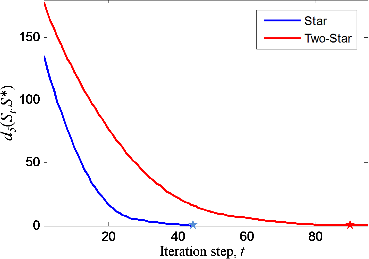
Figure 2: Convergence of the spectral pseudodistance $d_{k}(S_{t},S^{\ast})$ for the star graph (blue plot) and the two-stars graph (red plot), where $S^{\ast}$ is the spectrum of the desired graph and $S_{t}$ is the spectrum of $\mathcal{G}_{t}$.

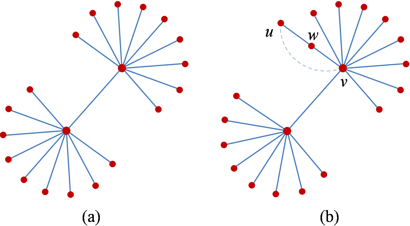
Figure 3: Structures of the two-stars network (a) and the network returned by our algorithm (b).

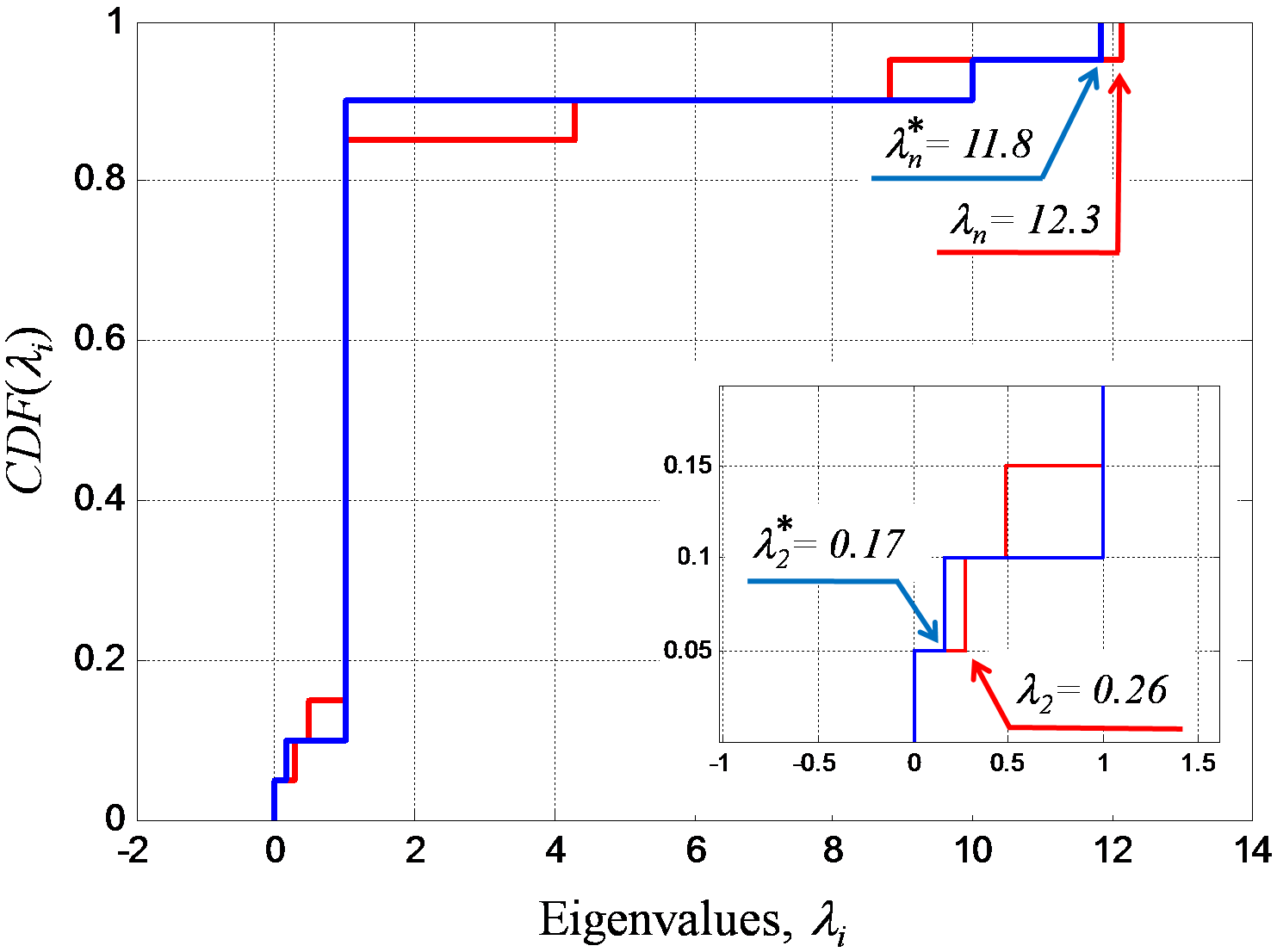
Figure 4: Empirical cumulative distribution functions for the eigenvalues of the two-stars graph (blue) and the graph returned by our algorithm (red). The subgraph in the lower right corner shows the CDF’s around the origin.

Example V.2 (Chain vs. ring networks)

In the next two simulations, we try to find graphs that match the spectral moments of (i) a ring graph and (ii) a chain graph. Starting from a random graph, we run our iterative algorithm to match the spectral moments of a chain graph with 20 nodes, $\left(m_{k}\right)_{k=1}^{5}=\left(1.9,5.6,18.4,63.6,226.4\right)$. In this case, the spectral pseudodistance converges to zero in finite time and the final topology is exactly the desired chain graph. On the other hand, if we try to match the spectral moments of the ring graph in Fig. 5 (a), with $\left(m_{k}\right)_{k=1}^{5}=\left(2,6,20,70,252\right)$, an exact reconstruction is very difficult to achieve. In Fig. 5 (b), we depict the graph returned by our algorithm, after 83 iterations. Note that since we are only allowing local structural modifications in our graph process, it is hard for our algorithm to replicate long cycles in the graph. On the other hand, although the structure of the resulting network is not the desired ring graph, its eigenvalue spectrum is remarkably close to that of a ring, as we can see in Fig. 6.

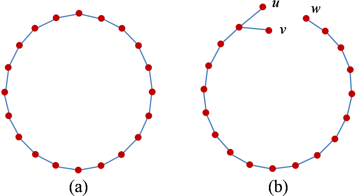
Figure 5: In (a) we observe a ring graph with 20 nodes. The topology returned by our iterative algorithm can be observed in (b).

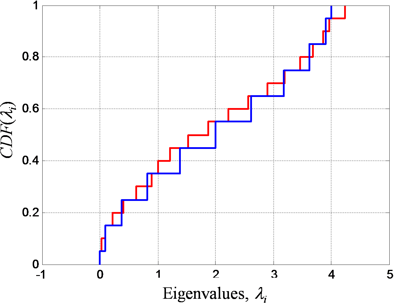
Figure 6: Empirical cumulative distribution of eigenvalues for the ring graph with 20 nodes (blue plot) and the topology returned by our algorithm in Fig. 5 (b) (red plot).

The above examples illustrate two limitations of our algorithm, namely, the existence of local minima in the graph evolution process and the inability of our algorithm to recover long cycles. Despite these limitations, our algorithm is able to find graph topologies with eigenvalue spectra remarkably close to the desired ones by matching five spectral moments only. Furthermore, the resulting topologies are structurally very similar to the desired ones, indicating that the spectral moments of the Laplacian matrix contains rich information about the structure of a network. In the next two examples, we show how our algorithm is also able to efficiently generate graphs matching the spectral properties of two popular synthetic network models: the Small-World [20] and the Scale-Free [21] networks.

Example V.3 (Small-Worlds)

The small-world model was proposed by Watts and Strogatz [20] to generate networks with high clustering coefficients and small average distance. We can generate a small-world network by following these steps: (1) take a ring graph with $n$ nodes, (2) connect each node in the ring to all its neighborhoods within a distance $k$, and (3) add random edges with a probability $p$. In this example, we generate a small-world network with $n=40$, $k=2$, and $p=3/n$. The first three spectral moments of a random realization of this network are $\left(m_{k}\right)_{k=1}^{3}=\left(6.55,51.9,457\right)$. Then, we run our algorithm to generate a graph whose first three spectral moments are close to those of the small-world network. After running our algorithm for $78$ iterations, we obtain a graph topology with a spectral pseudodistance very close to zero (in particular, $1.7e-3$) and an eigenvalue spectrum remarkably similar to that of the small-world network, as shown in Fig. 7.

Example V.4 (Power-Law)

Another popular model in the ‘Network Science’ literature is the scale-free network. This model was proposed by Barabási and Albert in [21] to explain the presence of heavy-tailed degree distributions in many real-world networks. In this example, we generate a random power-law network with $n=50$ nodes and $m=4$, where $m$ is a parameter that characterizes the average degree of the resulting network (see [21] for more details about this model). A random realization of this network presents the following sequence of moments: $\left(m_{k}\right)_{k=1}^{5}=(7.72,111,2.81e3,9.70e4,3.82e6)$. Then, after running our algorithm for $98$ iterations, we obtain a graph topology with a spectral pseudodistance very close to zero (in particular, $5.5e-2$). The eigenvalue spectrum of the resulting topology is remarkably similar to that of the small-world network, as shown in Fig. 8. Furthermore, we can compare the degree sequences of the power-law network and the topology generated by our algorithm. We compare these sequences, sorted in descending order, in Fig.9. We observe how the degree sequence of the topology obtained in our algorithm is remarkably close to that of the power-law network. This indicates that the spectral properties of a network contains rich information about the network structure, in particular, the first five spectral moments seems to highly constrain many relevant structural properties of the graph, such as the degree distribution.

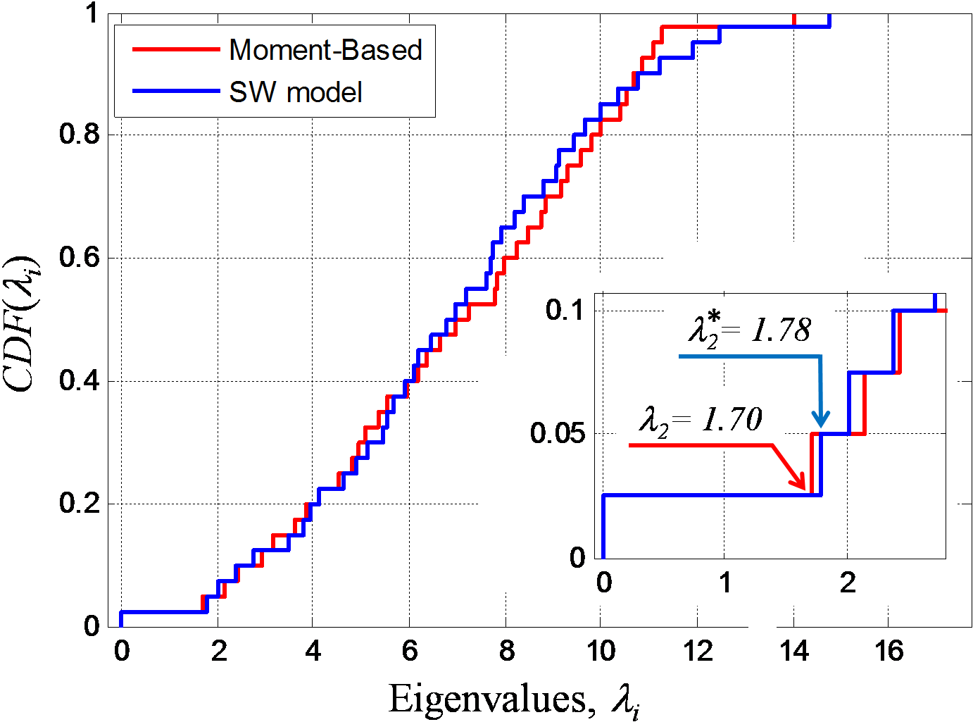
Figure 7: Empirical cumulative distribution for the eigenvalue spectrum of the small-world graph in Example V.3 (blue) and the topology resulting from our algorithm (red).

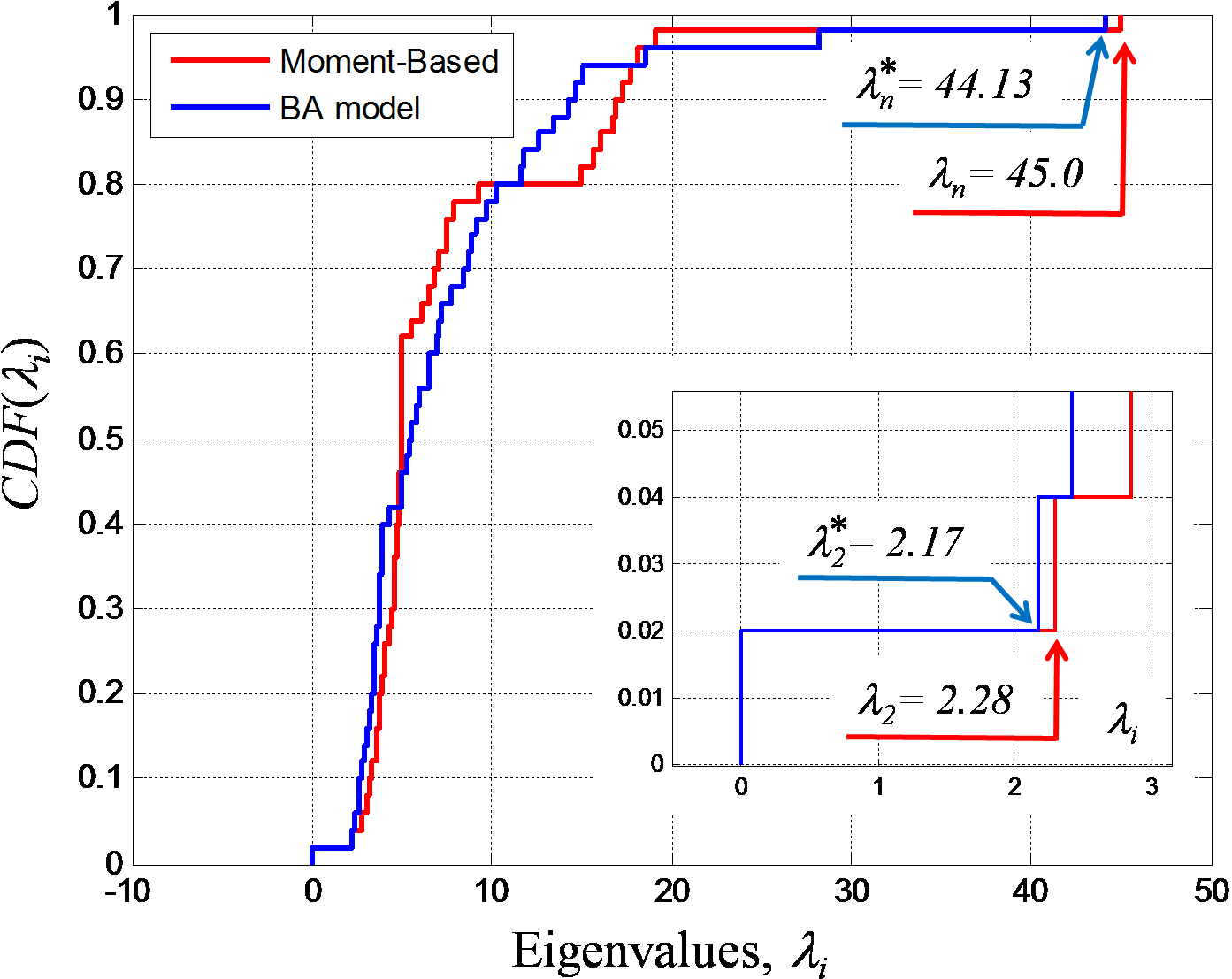
Figure 8: Empirical cumulative distribution for the eigenvalue spectrum of the power-law graph in Example V.4 (blue) and the topology resulting from our algorithm (red).

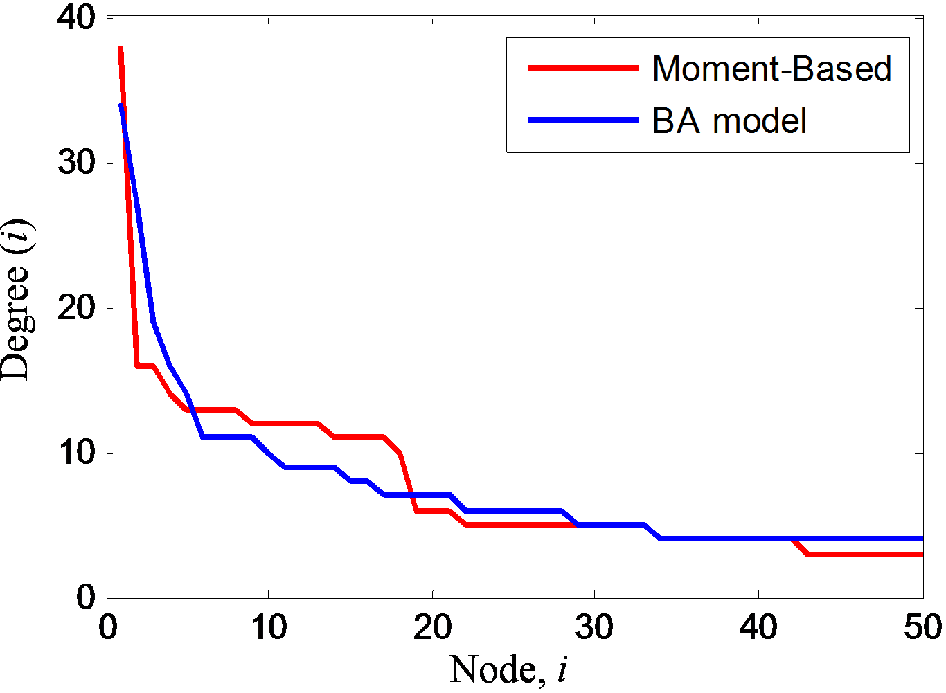
Figure 9: Degree sequences (in descending order) of the power-law graph in Example V.4 (blue) and the topology resulting from our algorithm (red).

VI Conclusions and Future Research

In this paper, we have described a fully decentralized algorithm that iteratively modifies the structure of a network of agents with the objective of controlling the spectral moments of the Laplacian matrix of the network. Although we assume that each agent has access to local information regarding the graph structure, we show that the group is able to collectively aggregate their local information to take a global optimal decision. This decision corresponds to the most beneficial link addition/deletion in order to minimize a distance function that involves the Laplacian spectral moments of the network. The aggregation of the local information is achieved via gossip algorithms, which are also used to ensure network connectivity throughout the evolution of the network.

Future work involves identifying sets of spectral moments that are reachable by our control algorithm. (We say that a sequence of spectral moments is reachable if there exists a graph whose moments match the sequence of moments.) Furthermore, we observed that fitting a set of low-order moments does not guarantee a good fit of the complete distribution of eigenvalues. In fact, there are important spectral parameters, such as the algebraic connectivity, that are not captured by a small set of spectral moments. Nevertheless, we observed in numerical simulations that fitting the first four moments of the eigenvalue spectrum often achieves a good reconstruction of the complete spectrum. Hence, a natural question is to describe the set of graphs most of whose spectral information is contained in a relatively small set of low-order moments.

Appendix A Proof of Theorem II.1

Theorem A.1

Consider two undirected (possibly weighted) graphs $G_{1}$ and $G_{2}$ with (real) eigenvalue spectra $S\left(G_{1}\right)=\{\lambda_{1}^{\left(1\right)}\leq...\leq\lambda_{n}^{\left(1\right)}\}$ and $S_{2}\left(G_{1}\right)=\{\lambda_{1}^{\left(2\right)}\leq...\leq\lambda_{n}^{\left(2\right)}\}$. Then, $\lambda_{i}^{\left(1\right)}=\lambda_{i}^{\left(2\right)}$ for all $1\leq i\leq n$ if and only if $m_{k}\left(G_{1}\right)=m_{k}\left(G_{2}\right)$ for $0\leq k\leq n-1$.

Proof:

The theorem states that the spectrum $S\left(A\right)=\left\{\lambda_{i}\right\}_{i=1}^{n}$ of any $n\times n$ symmetric matrix $A$ is uniquely characterized by its first $n-1$ spectral moments. First, we use Cayley-Hamilton theorem to prove that the first $n-1$ spectral moments of the spectrum $S$ characterize the whole infinite sequence of moments $\left(m_{k}\left(S\right)\right)_{k=0}^{\infty}$, as follows. Let $\phi\left(\lambda\right)\triangleq\det\left(\lambda I_{n}-A\right)=\lambda^{n}+\alpha_{n-1}\lambda^{n-1}+...+\alpha_{0}$, be the characteristic equation of $A$. Then, from Cayley-Hamilton, we have $\phi\left(A\right)=0$. Multiplying $\phi\left(A\right)$ by $\frac{1}{n}A^{t}$, and applying the trace operator, we have that,

$$\frac{1}{n}\text{Trace}\left[A^{t}\phi\left(A\right)\right] = \frac{1}{n}\text{Trace}\left(A^{t+n}\right)+\alpha_{n-1}\frac{1}{n}\text{Trace}\left(A^{t+n-1}\right)+...+\alpha_{0}\frac{1}{n}\text{Trace}\left(A^{t}\right)$$

$$= m_{t+n}\left(A\right)+\alpha_{n-1}m_{t+n-1}\left(A\right)+...+\alpha_{0}m_{t}\left(A\right)=0,$$

for all $t\in\mathbb{N}$. Therefore, given the sequence of moments $\left(m_{k}\left(A\right)\right)_{k=0}^{n-1}$, we can use the recursion

$$m_{t+n}\left(A\right)=-\alpha_{n-1}m_{t+n-1}\left(A\right)-...-\alpha_{1}m_{t+1}\left(A\right)-\alpha_{0}m_{t}\left(A\right),$$

to uniquely characterize the infinite sequence of moments $\left(m_{k}\left(A\right)\right)_{k=0}^{\infty}$.

Second, we prove that the infinite sequence of moments $\left(m_{k}\left(A\right)\right)_{k=0}^{\infty}$ uniquely characterizes the eigenvalue spectrum. Let us define the spectral measure of the matrix $A$ with real eigenvalues $\lambda_{1}\leq\lambda_{2}\leq...\leq\lambda_{n}$, as

$$\mu_{A}\left(x\right)=\sum_{i=1}^{n}\delta\left(x-\lambda_{i}\right),$$

where $\delta\left(\bullet\right)$ is the Dirac delta function. In what follows, we prove that the spectral measure of $A$ is uniquely characterized by its infinite sequence of spectral moments using Carleman’s condition [22]. Since there is a trivial bijection between the eigenvalue spectrum of $A$ and its spectral measure, uniqueness of the spectral measure imply uniqueness of the eigenvalue spectrum.

Carleman’s condition states that a measure $\mu$ on $\mathbb{R}$ is uniquely characterized by its infinite sequence of moments $\left(M_{k}\left(\mu\right)\right)_{k=1}^{\infty}$ if (i) $M_{k}\left(\mu\right)<\infty$ for all $k\in\mathbb{N}$, and (ii)

$$\sum_{s=1}^{\infty}\left(M_{2s}\left(\mu\right)\right)^{-1/2s}=\infty.$$

In our case, the moments of the spectral measure $\mu_{A}$ are

$$M_{k}\left(\mu_{A}\right) = \int_{-\infty}^{+\infty}x^{k}d\mu_{A}\left(x\right)$$

$$= \sum_{i=1}^{n}\lambda_{i}^{k}=n~{}m_{k}\left(A\right).$$

These moments satisfy: (i) $M_{k}\left(\mu_{A}\right)\leq n\lambda_{n}^{k}<\infty$, for any finite matrix $A$, and (ii)

$$\sum_{s=1}^{\infty}\left(M_{2s}\left(\mu_{A}\right)\right)^{-1/2s} = \sum_{s=1}^{\infty}\left(\sum_{i=1}^{n}\lambda_{i}^{2s}\right)^{-1/2s}$$

$$\geq \sum_{s=1}^{\infty}\left(\lambda_{n}^{2s}\right)^{-1/2s}$$

$$= \sum_{s=1}^{\infty}\lambda_{n}^{-1}=\infty,$$

for any $A\neq 0$. As a consequence, the spectral measure of any finite matrix $A\neq 0$ with real eigenvalues is uniquely characterized by $\left(M_{k}\left(\mu_{A}\right)\right)_{k=0}^{\infty}$. Since, $M_{k}\left(\mu_{A}\right)=n~{}m_{k}\left(A\right)$, we have that the sequence of moments $\left(m_{k}\left(A\right)\right)_{k=0}^{n-1}$ uniquely characterizes $\left(M_{k}\left(\mu_{A}\right)\right)_{k=0}^{\infty}$. Therefore, the sequence of moments $\left(m_{k}\left(A\right)\right)_{k=0}^{n-1}$ uniquely characterize the spectral measure $\mu_{A}$ and the real eigenvalue spectrum $S=\left\{\lambda_{i}\right\}_{i=1}^{n}$.

References

- [1] N. Wiener, The Mathematics of Self-Organising Systems. Recent Developments in Information and Decision Processes, Macmillan, 1962.
- [2] H. Haken, Synergetics: An Introduction, 3rd Edition, Springer-Verlag, 1983.
- [3] M.O. Jackson, Social and Economic Networks, Princeton University Press, 2008.
- [4] V.M. Preciado, Spectral Analysis for Stochastic Models of Large-Scale Complex Dynamical Networks, Ph.D. dissertation, Dept. Elect. Eng. Comput. Sci., MIT, Cambridge, MA, 2008.
- [5] L.M. Pecora and T.L. Carroll, “Master Stability Functions for Synchronized Coupled Systems,” Physics Review Letters, vol. 80, pp. 2109-2112, 1998.
- [6] V.M. Preciado and G.C. Verghese, “Synchronization in Generalized Erdös-Rényi Networks of Nonlinear Oscillators,” Proc. of the 44th IEEE Conference on Decision and Control, pp. 4628-4633, 2005.
- [7] N.A. Lynch, Distributed Algorithms, Morgan Kaufmann Publishers, 1997.
- [8] A. Fax and R. M. Murray, “Information Flow and Cooperative Control of Vehicle Formations,” IEEE Transactions on Automatic Control, vol. 49, pp. 1465-1476, 2004.
- [9] R. Olfati-Saber and R. M. Murray, “Consensus Problems in Networks of Agents with Switching Topology and Time-Delays,” IEEE Transactions on Automatic Control, vol. 49, pp. 1520-1533, 2004.
- [10] R. Grone, R. Merris, and V.S. Sunder, “The Laplacian Spectrum of a Graph,” SIAM Journal Matrix Analysis and Applications, vol. 11, pp. 218-238, 1990.
- [11] A. Ghosh and S. Boyd, “Growing Well-Connected Graphs,” Proc. of the 45th IEEE Conference on Decision and Control, pp. 6605-6611, 2006.
- [12] Y. Kim and M. Mesbahi, “On Maximizing the Second-Smallest Eigenvalue of a State Dependent Graph Laplacian,” IEEE Transactions on Automatic Control, vol. 51, pp. 116-120, 2006.
- [13] M.C. DeGennaro and A. Jadbabaie, “Decentralized Control of Connectivity for Multi-Agent Systems,” Proc. of the 45th IEEE Conference on Decision and Control, San Diego, CA, Dec. 2006, pp. 3628-3633.
- [14] N. Biggs, Algebraic Graph Theory, Cambridge University Press, 2nd Edition, 1993.
- [15] V.M. Preciado and G.C. Verghese, “Low-Order Spectral Analysis of the Kirchhoff Matrices for a Probabilistic Graph with Prescribed Expected Degree Sequence,” IEEE Transactions on Circuits and Systems I, vol. 56, pp, 1231-1240, 2009.
- [16] D.M. Cvetković, M. Doob, and H. Sachs, Spectra of Graphs, 3 Edition, Wiley-VCH, 1998.
- [17] J. H. Wilkinson, The Algebraic Eigenvalue Problem, Oxford University Press, 1965.
- [18] J. Cortes, “Distributed Algorithms for Reaching Consensus on General Functions,” Automatica, vol. 44, pp. 726-737, 2008.
- [19] M. M. Zavlanos and G. J. Pappas, “Distributed Connectivity Control of Mobile Networks,” IEEE Transactions on Robotics, vol. 24, pp. 1416-1428, 2008.
- [20] D.J. Watts and S. Strogatz, “Collective Dynamics of Small World Networks,” Nature, vol. 393, pp. 440-42, 1998.
- [21] A. L. Barabási and R. Albert, “Emergence of Scaling in Random Networks,” Science, vol. 285, pp. 509-512, 1999.
- [22] N.I. Akhiezer, The Classical Moment Problem and Some Related Questions in Analysis, Oliver & Boyd, 1965.