Abstract

We evaluate two-body decay modes of charginos in the Minimal Supersymmetric Standard Model with complex parameters (cMSSM). Assuming heavy scalar quarks we take into account all decay channels involving charginos, neutralinos, (scalar) leptons, Higgs bosons and Standard Model gauge bosons. The evaluation of the decay widths is based on a full one-loop calculation including hard and soft QED radiation. Special attention is paid to decays involving the Lightest Supersymmetric Particle (LSP), i.e. the lightest neutralino, or a neutral or charged Higgs boson. The higher-order corrections of the chargino decay widths involving the LSP can easily reach a level of about $\pm 10\%$, while the corrections to the decays to Higgs bosons are slightly smaller, translating into corrections of similar size in the respective branching ratios. These corrections are important for the correct interpretation of LSP and Higgs production at the LHC and at a future linear $e^{+}e^{-}$ collider. The results will be implemented into the Fortran code FeynHiggs.

1 Introduction

One of the important tasks at the LHC is to search for physics beyond the Standard Model (SM), where the Minimal Supersymmetric Standard Model (MSSM) [1] is one of the leading candidates. Two related important tasks are investigating the mechanism of electroweak symmetry breaking, as well as the production and measurement of the properties of Cold Dark Matter (CDM). The most frequently investigated models for electroweak symmetry breaking are the Higgs mechanism within the SM and within the MSSM. The latter also offers a natural candidate for CDM, the Lightest Supersymmetric Particle (LSP), i.e. the lightest neutralino, $\tilde{\chi}^{0}_{1}$ [2]. Supersymmetry (SUSY) predicts two scalar partners for all SM fermions as well as fermionic partners to all SM bosons. Contrary to the case of the SM, in the MSSM two Higgs doublets are required. This results in five physical Higgs bosons instead of the single Higgs boson in the SM. These are the light and heavy ${\cal CP}$-even Higgs bosons, $h$ and $H$, the ${\cal CP}$-odd Higgs boson, $A$, and the charged Higgs bosons, $H^{\pm}$. In the MSSM with complex parameters (cMSSM) the three neutral Higgs bosons mix [3, 4, 5], giving rise to the states $h_{1},h_{2},h_{3}$.

If SUSY is realized in nature and the scalar quarks and/or the gluino are in the kinematic reach of the LHC, it is expected that these strongly interacting particles are copiously produced. The primarily produced strongly interacting particles subsequently decay via cascades to SM particles and (if $R$-parity conservation is assumed, as we do) the LSP. One step in these decay chains is often the decay of a chargino, $\tilde{\chi}^{\pm}_{1,2}$, to a SM particle and the LSP, or as a competing process the chargino decay to another SUSY particle accompanied by a SM particle. Also neutral and charged Higgs bosons can be produced this way. Via these decays some characteristics of the LSP and/or Higgs bosons can be measured, see, e.g., Refs. [6, 7] and references therein. At any future $e^{+}e^{-}$ collider (such as ILC or CLIC) a precision determination of the properties of the observed particles is expected [8, 9]. (For combined LHC/ILC analyses and further prospects see Ref. [10].) Thus, if kinematically accessible, the pair production of charginos with a subsequent decay to the LSP and/or Higgs bosons can yield important information about the lightest neutralino and the Higgs sector of the model.

In order to yield a sufficient accuracy, one-loop corrections to the various chargino decay modes have to be considered. In this paper we evaluate full one-loop corrections to chargino decays in the cMSSM. If scalar quarks are sufficiently heavy (as in many GUT based models such as CMSSM, GMSB or AMSB, see for instance Ref. [11]) a chargino decay to a quark and a scalar quark is kinematically forbidden. Assuming heavy squarks we calculate the full one-loop correction to all two body decay modes (which are non-zero at the tree-level),

$$\Gamma(\tilde{\chi}^{-}_{i}\to\tilde{\chi}^{0}_{j}H^{-})\qquad(i=1,2,\;j=1,2,3,4)~{},$$ (1)

$$\Gamma(\tilde{\chi}^{-}_{i}\to\tilde{\chi}^{0}_{j}W^{-})\qquad(i=1,2,\;j=1,2,3,4)~{},$$ (2)

$$\Gamma(\tilde{\chi}^{-}_{2}\to\tilde{\chi}^{-}_{1}h_{k})\qquad(k=1,2,3)~{},$$ (3)

$$\Gamma(\tilde{\chi}^{-}_{2}\to\tilde{\chi}^{-}_{1}Z)~{},$$ (4)

$$\Gamma(\tilde{\chi}^{-}_{i}\to\bar{\nu}_{l}\,\tilde{l}_{k}^{-})\qquad(i=1,2,\;l=e,\mu,\tau,\;k=1,2)~{},$$ (5)

$$\Gamma(\tilde{\chi}^{-}_{i}\to{l}^{-}\,\tilde{\nu}_{l}^{\dagger})\qquad(i=1,2,\;l=e,\mu,\tau)~{}.$$ (6)

The total width is defined as the sum of the channels (1) to (6), where for a given parameter point several channels may be kinematically forbidden.

As explained above, we are especially interested in the branching ratios (BR) of the decays involving a Higgs boson, Eqs. (1), (3) as part of an evaluation of a Higgs production cross section, and/or involving the LSP, Eqs. (1), (2) as part of the measurement of CDM properties at the LHC. Consequently, it is not necessary to investigate three- or four-body decay modes. These only play a significant role once the two-body modes are kinematically forbidden, and thus the relevant BR’s are zero. The same applies to two-body decay modes that exist only at the one-loop level, such as $\tilde{\chi}^{\pm}_{2}\to\tilde{\chi}^{\pm}_{1}\gamma$ (see, for instance, Ref. [13]). While this channel is of ${\cal O}(\alpha^{2})$, the size of the one-loop corrections to Eqs. (1) to (6) is of ${\cal O}(\alpha)$. We have numerically verified that the contribution of $\Gamma(\tilde{\chi}^{\pm}_{2}\to\tilde{\chi}^{\pm}_{1}\gamma)$ to the total width is completely negligible.

Tree-level results for the decays of charginos in the MSSM were presented in Refs. [12, 13, 14]. Higher-order corrections to chargino decays have been evaluated in various analyses over the last decade. However, they were either restricted to one specific channel or only a very restricted set of parameters were analyzed, and in many cases only parts of the one-loop calculation have been performed. More specifically, the available literature comprises the following. First order electroweak corrections to the partial decay widths of charginos in the MSSM with real parameters (rMSSM) where derived: for the two-body decays into a neutralino/chargino and $W/Z$ boson including only third generation quark-squark exchange diagrams [15], for the three-body decays into the LSP and quarks, including corrections to the masses of third generation fermions and SUSY particles [16], and for the three-body leptonic decays at full one-loop order in Ref. [17]. The one-loop electroweak corrections to all two-body decay channels of charginos, evaluated in an on-shell renormalization scheme, have been implemented in the code SloopS [18]. In Ref. [19] a large set of two-body and three-body decay channels of charginos including full one-loop corrections has been calculated using the code GRACE/SUSY-loop, but only a very limited set of numerical results have been published. However, Ref. [18] has compared its results on the partial widths with those of Ref. [19] and concluded that the latter uses a renormalization scheme which leads to too large corrections. The code SDECAY [20] also includes all two-body decays of charginos. However, no radiative corrections to these decay channels have been included so far. A full one-loop calculation of the electroweak corrections to the partial width of the decay of a chargino into a neutralino and a $W$ boson in the MSSM and NMSSM is presented in Ref. [21], and made available with the code CNNDecays. A brief comparison with this calculation can be found in Sect. 3. In the cMSSM only the decay of charginos into a neutralino and a $W$ boson has been studied. In Ref. [22] a partial one-loop calculation of rate asymmetries of $\tilde{\chi}^{\mp}_{i}\to\tilde{\chi}^{0}_{1}W^{\mp}$ has been performed, including contributions from the third generation quarks, while Ref. [23] evaluated this ${\cal CP}$-violating asymmetry at the full one-loop level, highlighting the relevance of the contribution from the chargino wave function corrections. However, a complete one-loop result for the two-body total decay width in the cMSSM is missing so far.

In this paper we present for the first time a full one-loop calculation for all non-hadronic two-body decay channels of a chargino, taking into account soft and hard QED radiation, simultaneously and consistently evaluated in the cMSSM. In Sect. 2 we review the relevant sectors of the cMSSM and their renormalization. Details about the calculation can be found in Sect. 3, and the numerical results for all decay channels are presented in Sect. 4. The conclusions can be found in Sect. 5. The evaluation of the branching ratios of the charginos will be implemented into the Fortran code FeynHiggs [24, 25, 26, 27].

2 The relevant sectors of the complex MSSM

All the channels (1) – (6) are calculated at the one-loop level, including real QED radiation. This requires the simultaneous renormalization of several sectors of the cMSSM. In the following subsections we briefly review these sectors. Details about the renormalization of most of the sectors can be found in Ref. [28]. Here we only review the renormalization that can not be found explicitly in Ref. [28].

2.1 The lepton/slepton sector of the cMSSM

For the evaluation of the one-loop contributions to the decay channels in Eqs. (5), (6) a renormalization of the scalar lepton ($\tilde{l}$) and neutrino ($\tilde{\nu_{l}}$) sector is needed (we assume no generation mixing and discuss the case for one generation only). The bilinear part of the $\tilde{l}$ and $\tilde{\nu_{l}}$ Lagrangian,

$${\cal L}_{\tilde{l}/\tilde{\nu_{l}}}^{\text{mass}} =-\begin{pmatrix}\tilde{l}_{L}^{\dagger},\tilde{l}_{R}^{\dagger}\end{pmatrix}{\mathbf{M}}_{\tilde{l}}\begin{pmatrix}\tilde{l}_{L}\\ \tilde{l}_{R}\end{pmatrix}-\begin{pmatrix}\tilde{\nu_{l}}^{\dagger}\end{pmatrix}{\mathbf{M}}_{\tilde{\nu_{l}}}\begin{pmatrix}\tilde{\nu_{l}}\end{pmatrix}~{},$$ (7)

contains the slepton and sneutrino mass matrices ${\mathbf{M}}_{\tilde{l}}$ and ${\mathbf{M}}_{\tilde{\nu_{l}}}$, given by

$${\mathbf{M}}_{\tilde{l}} =\begin{pmatrix}M_{\tilde{l}_{L}}^{2}+m_{l}^{2}+M_{Z}^{2}c_{2\beta}(I_{l}^{3}-Q_{l}s_{\mathrm{w}}^{2})&m_{l}X_{l}^{*}\\[1.99997pt] m_{l}X_{l}&M_{\tilde{l}_{R}}^{2}+m_{l}^{2}+M_{Z}^{2}c_{2\beta}Q_{l}s_{\mathrm{w}}^{2}\end{pmatrix}~{},$$ (8)

$${\mathbf{M}}_{\tilde{\nu_{l}}} =M_{\tilde{l}_{L}}^{2}+I_{\nu}^{3}c_{2\beta}M_{Z}^{2}$$ (9)

with

$$X_{l} =A_{l}-\mu^{*}\tan\beta~{}.$$ (10)

$M_{\tilde{l}_{L}}$ and $M_{\tilde{l}_{R}}$ are the soft SUSY-breaking mass parameters, where $M_{\tilde{l}_{L}}$ is equal for all members of an $SU(2)_{L}$ doublet. $m_{l}$ and $Q_{l}$ are, respectively, the mass and the charge of the corresponding lepton, $I_{l/\nu}^{3}$ denotes the isospin of $l/\nu$, and $A_{l}$ is the trilinear soft-breaking parameter. $M_{Z}$ and $M_{W}$ are the masses of the $Z$ and $W$ boson, $c_{\mathrm{w}}=M_{W}/M_{Z}$, and $s_{\mathrm{w}}=\sqrt{1-c_{\mathrm{w}}^{2}}$. Finally we use the short-hand notations $c_{x}=\cos(x)$, $s_{x}=\sin(x)$. The mass matrix ${\mathbf{M}}_{\tilde{l}}$ can be diagonalized with the help of a unitary transformation ${{\mathbf{U}}}_{\tilde{l}}$,

$${\mathbf{D}}_{\tilde{l}} ={\mathbf{U}}_{\tilde{l}}\,{\mathbf{M}}_{\tilde{l}}\,{{\mathbf{U}}}_{\tilde{l}}^{\dagger}=\begin{pmatrix}m_{\tilde{l}_{1}}^{2}&0\\ 0&m_{\tilde{l}_{2}}^{2}\end{pmatrix}~{},\qquad{{\mathbf{U}}}_{\tilde{l}}=\begin{pmatrix}U_{\tilde{l}_{11}}&U_{\tilde{l}_{12}}\\ U_{\tilde{l}_{21}}&U_{\tilde{l}_{22}}\end{pmatrix}~{}.$$ (11)

The mass eigenvalues depend only on $|X_{l}|$. The scalar lepton masses will always be mass ordered, i.e. $m_{\tilde{l}_{1}}\leq m_{\tilde{l}_{2}}$:

$$m_{\tilde{l}_{1,2}}^{2} =\frac{1}{2}\left(M_{\tilde{l}_{L}}^{2}+M_{\tilde{l}_{R}}^{2}\right)+m_{l}^{2}+\frac{1}{2}I_{l}^{3}c_{2\beta}M_{Z}^{2}$$ (12)

$$\quad\mp\frac{1}{2}\sqrt{\left[M_{\tilde{l}_{L}}^{2}-M_{\tilde{l}_{R}}^{2}+M_{Z}^{2}c_{2\beta}(I_{l}^{3}-2Q_{l}s_{\mathrm{w}}^{2})\right]^{2}+4m_{l}^{2}|X_{l}|^{2}}~{},$$

$$m_{\tilde{\nu_{l}}}^{2} =M_{\tilde{l}_{L}}^{2}+I_{\nu}^{3}c_{2\beta}M_{Z}^{2}~{}.$$ (13)

2.1.1 Renormalization

The parameter renormalization can be performed as follows,

$${\mathbf{M}}_{\tilde{l}} \to{\mathbf{M}}_{\tilde{l}}+\delta{\mathbf{M}}_{\tilde{l}}~{},$$ (14)

$${\mathbf{M}}_{\tilde{\nu_{l}}} \to{\mathbf{M}}_{\tilde{\nu_{l}}}+\delta{\mathbf{M}}_{\tilde{\nu_{l}}}$$ (15)

which means that the parameters in the mass matrix ${\mathbf{M}}_{\tilde{l}}$ are replaced by the renormalized parameters and a counterterm. After the expansion $\delta{\mathbf{M}}_{\tilde{l}}$ contains the counterterm part,

$$\delta{\mathbf{M}}_{\tilde{l}_{11}} =\delta M_{\tilde{l}_{L}}^{2}+2m_{l}\delta m_{l}-M_{Z}^{2}c_{2\beta}\,Q_{l}\,\delta s_{\mathrm{w}}^{2}+(I_{l}^{3}-Q_{l}s_{\mathrm{w}}^{2})(c_{2\beta}\,\delta M_{Z}^{2}+M_{Z}^{2}\,\delta c_{2\beta})~{},$$ (16)

$$\delta{\mathbf{M}}_{\tilde{l}_{12}} =(A_{l}^{*}-\mu\tan\beta)\,\delta m_{l}+m_{l}(\delta A_{l}^{*}-\mu\,\delta\tan\beta-\tan\beta\,\delta\mu)~{},$$ (17)

$$\delta{\mathbf{M}}_{\tilde{l}_{21}} =\delta{\mathbf{M}}_{\tilde{l}_{12}}^{*}~{},$$ (18)

$$\delta{\mathbf{M}}_{\tilde{l}_{22}} =\delta M_{\tilde{l}_{R}}^{2}+2m_{l}\delta m_{l}+M_{Z}^{2}c_{2\beta}\,Q_{l}\,\delta s_{\mathrm{w}}^{2}+Q_{l}s_{\mathrm{w}}^{2}(c_{2\beta}\,\delta M_{Z}^{2}+M_{Z}^{2}\,\delta c_{2\beta})~{},$$ (19)

$$\delta{\mathbf{M}}_{\tilde{\nu_{l}}} =\delta M_{\tilde{l}_{L}}^{2}+I_{\nu}^{3}(c_{2\beta}\,\delta M_{Z}^{2}+M_{Z}^{2}\,\delta c_{2\beta})~{}.$$ (20)

Another possibility for the parameter renormalization of the sleptons is to start out with the physical parameters which corresponds to the replacement:

$${\mathbf{U}}_{\tilde{l}}\,{\mathbf{M}}_{\tilde{l}}\,{{\mathbf{U}}}_{\tilde{l}}^{\dagger} \to{\mathbf{U}}_{\tilde{l}}\,{\mathbf{M}}_{\tilde{l}}\,{{\mathbf{U}}}_{\tilde{l}}^{\dagger}+{\mathbf{U}}_{\tilde{l}}\,\delta{\mathbf{M}}_{\tilde{l}}\,{{\mathbf{U}}}_{\tilde{l}}^{\dagger}=\begin{pmatrix}m_{\tilde{l}_{1}}^{2}&Y_{l}\\ Y_{l}^{*}&m_{\tilde{l}_{2}}^{2}\end{pmatrix}+\begin{pmatrix}\delta m_{\tilde{l}_{1}}^{2}&\delta Y_{l}\\ \delta Y_{l}^{*}&\delta m_{\tilde{l}_{2}}^{2}\end{pmatrix}$$ (21)

where $\delta m_{\tilde{l}_{1}}$ and $\delta m_{\tilde{l}_{2}}$ are the counterterms of the slepton masses. $\delta Y_{l}$ is the counterterm to the slepton mixing parameter $Y_{l}$ (which vanishes at tree-level, $Y_{l}=0$, and corresponds to the off-diagonal entries in ${\mathbf{D}}_{\tilde{l}}={\mathbf{U}}_{\tilde{l}}\,{\mathbf{M}}_{\tilde{l}}\,{{\mathbf{U}}}_{\tilde{l}}^{\dagger}$, Eq. (11)). Using Eq. (21) one can express $\delta{\mathbf{M}}_{\tilde{l}}$ by the counterterms $\delta m_{\tilde{l}_{1}}^{2}$, $\delta m_{\tilde{l}_{2}}^{2}$ and $\delta Y_{l}$. Especially for $\delta{\mathbf{M}}_{\tilde{l}_{12}}$ one finds

$$\delta{\mathbf{M}}_{{\tilde{l}}_{12}} =U^{*}_{\tilde{l}_{11}}U_{\tilde{l}_{12}}(\delta m_{\tilde{l}_{1}}^{2}-\delta m_{\tilde{l}_{2}}^{2})+U^{*}_{\tilde{l}_{11}}U_{\tilde{l}_{22}}\delta Y_{l}+U_{\tilde{l}_{12}}U^{*}_{\tilde{l}_{21}}\delta Y_{l}^{*}~{}.$$ (22)

In the following the relation given by Eqs. (17) and (22) will be used to express either $\delta Y_{l}$, $\delta A_{l}$ or $\delta m_{l}$ by the other counterterms.

For the field renormalization the following procedure is applied,

$$\begin{pmatrix}\tilde{l}_{1}\\ \tilde{l}_{2}\end{pmatrix} \to\left({\rm 1\kern-1.19995pt\rule{0.3pt}{6.45831pt}\raisebox{0.0pt}{\rule{1.00006pt}{0.3pt}}}+\frac{1}{2}\delta{\mathbf{Z}}_{\tilde{l}}\right)\begin{pmatrix}\tilde{l}_{1}\\ \tilde{l}_{2}\end{pmatrix}~{}~{}{\rm with}~{}~{}\delta{\mathbf{Z}}_{\tilde{l}}=\begin{pmatrix}\delta Z_{\tilde{l}_{11}}&\delta Z_{\tilde{l}_{12}}\\ \delta Z_{\tilde{l}_{21}}&\delta Z_{\tilde{l}_{22}}\end{pmatrix}~{},$$ (23)

$$\tilde{\nu_{l}} \to\left(1+\tfrac{1}{2}\delta Z_{\tilde{\nu_{l}}}\right)\tilde{\nu_{l}}~{}.$$ (24)

This yields for the renormalized self-energies

$$\hat{\Sigma}_{\tilde{l}_{11}}(k^{2}) =\Sigma_{\tilde{l}_{11}}(k^{2})+\tfrac{1}{2}(k^{2}-m_{\tilde{l}_{1}}^{2})(\delta Z_{\tilde{l}_{11}}+\delta Z_{\tilde{l}_{11}}^{*})-\delta m_{\tilde{l}_{1}}^{2}~{},$$ (25)

$$\hat{\Sigma}_{\tilde{l}_{12}}(k^{2}) =\Sigma_{\tilde{l}_{12}}(k^{2})+\tfrac{1}{2}(k^{2}-m_{\tilde{l}_{1}}^{2})\delta Z_{\tilde{l}_{12}}+\tfrac{1}{2}(k^{2}-m_{\tilde{l}_{2}}^{2})\delta Z_{\tilde{l}_{21}}^{*}-\delta Y_{l}~{},$$ (26)

$$\hat{\Sigma}_{\tilde{l}_{21}}(k^{2}) =\Sigma_{\tilde{l}_{21}}(k^{2})+\tfrac{1}{2}(k^{2}-m_{\tilde{l}_{1}}^{2})\delta Z_{\tilde{l}_{12}}^{*}+\tfrac{1}{2}(k^{2}-m_{\tilde{l}_{2}}^{2})\delta Z_{\tilde{l}_{21}}-\delta Y_{l}^{*}~{},$$ (27)

$$\hat{\Sigma}_{\tilde{l}_{22}}(k^{2}) =\Sigma_{\tilde{l}_{22}}(k^{2})+\tfrac{1}{2}(k^{2}-m_{\tilde{l}_{2}}^{2})(\delta Z_{\tilde{l}_{22}}+\delta Z_{\tilde{l}_{22}}^{*})-\delta m_{\tilde{l}_{2}}^{2}~{},$$ (28)

$$\hat{\Sigma}_{\tilde{\nu_{l}}}(k^{2}) =\Sigma_{\tilde{\nu_{l}}}(k^{2})+\tfrac{1}{2}(k^{2}-m_{\tilde{\nu}_{l}}^{2})(\delta Z_{\tilde{\nu_{l}}}+\delta Z_{\tilde{\nu_{l}}}^{*})-\delta m_{\tilde{\nu}_{l}}^{2}~{}.$$ (29)

In order to complete the lepton/slepton sector renormalization also for the corresponding lepton (i.e. its mass, $m_{l}$, and the lepton fields $l_{L}$, $l_{R}$, $\nu_{L}$) renormalization constants have to be introduced:

$$m_{l} \to m_{l}+\delta m_{l}~{},$$ (30)

$$l_{L/R} \to(1+\tfrac{1}{2}\delta Z_{l}^{L/R})\,l_{L/R}~{},$$ (31)

$$\nu_{L} \to(1+\tfrac{1}{2}\delta Z_{\nu})\,\nu_{L}~{},$$ (32)

with $\delta m_{l}$ being the lepton mass counterterm and $\delta Z_{l}^{L}$ and $\delta Z_{l}^{R}$ being the $Z$ factors of the left-handed and the right-handed charged lepton fields, respectively; $\delta Z_{\nu}$ is the neutrino field renormalization. Then the renormalized self energy $\hat{\Sigma}_{l}$ can be decomposed into left/right-handed and scalar left/right-handed parts, ${\Sigma}_{l}^{L/R}$ and ${\Sigma}_{l}^{SL/SR}$, respectively, while only the left-handed part exists for the self energy $\hat{\Sigma}_{\nu}$ of the massless neutrino

$$\hat{\Sigma}_{l}(k) =\not\!k\,{\omega}_{-}\hat{\Sigma}_{l}^{L}(k^{2})+\not\!k\,{\omega}_{+}\hat{\Sigma}_{l}^{R}(k^{2})+{\omega}_{-}\hat{\Sigma}_{l}^{SL}(k^{2})+{\omega}_{+}\hat{\Sigma}_{l}^{SR}(k^{2})~{},$$ (33)

$$\hat{\Sigma}_{\nu}(k) =\not\!k\,{\omega}_{-}\hat{\Sigma}_{\nu}^{L}(k^{2})~{},$$ (34)

where the components are given by

$$\hat{\Sigma}_{l}^{L/R}(k^{2}) ={\Sigma}_{l}^{L/R}(k^{2})+\frac{1}{2}(\delta Z_{l}^{L/R}+{\delta Z_{l}^{L/R}}^{*})~{},$$ (35)

$$\hat{\Sigma}_{l}^{SL}(k^{2}) ={\Sigma}_{l}^{SL}(k^{2})-\frac{m_{l}}{2}(\delta Z_{l}^{L}+{\delta Z_{l}^{R}}^{*})-\delta m_{l}~{},$$ (36)

$$\hat{\Sigma}_{l}^{SR}(k^{2}) ={\Sigma}_{l}^{SR}(k^{2})-\frac{m_{l}}{2}(\delta Z_{l}^{R}+{\delta Z_{l}^{L}}^{*})-\delta m_{l}~{},$$ (37)

$$\hat{\Sigma}_{\nu}^{L}(k^{2}) ={\Sigma}_{\nu}^{L}(k^{2})+\frac{1}{2}(\delta Z_{\nu}^{L}+{\delta Z_{\nu}^{L}}^{*})~{},$$ (38)

and ${\omega}_{\pm}=\frac{1}{2}({\rm 1\kern-1.19995pt\rule{0.3pt}{6.45831pt}\raisebox{0.0pt}{\rule{1.00006pt}{0.3pt}}}\pm\gamma_{5})$ are the right- and left-handed projectors, respectively. Note that $\widetilde{\mathop{\mathrm{Re}}}\hat{\Sigma}_{l}^{SR}(k^{2})=(\widetilde{\mathop{\mathrm{Re}}}\hat{\Sigma}_{l}^{SL}(k^{2}))^{*}$ holds due to ${\cal CPT}$ invariance.

2.1.2 The neutrino/sneutrino sector

We follow closely the renormalization presented in Ref. [30, 28], slightly modified to be applicable to the lepton/slepton sector.

• The neutrino is defined on-shell (OS), yielding the one-loop field renormalization

  $$\mathop{\mathrm{Re}}\delta Z_{\nu} =-\widetilde{\mathop{\mathrm{Re}}}\Sigma_{\nu}(0)~{},$$ (39)

  $$\mathop{\mathrm{Im}}\delta Z_{\nu} =0~{}.$$ (40)

  $\widetilde{\mathop{\mathrm{Re}}}$ denotes the real part with respect to contributions from the loop integral, but leaves the complex couplings unaffected.

• The $\tilde{\nu_{l}}$ mass is defined OS,

  $$\widetilde{\mathop{\mathrm{Re}}}\hat{\Sigma}_{\tilde{\nu_{l}}}(m_{\tilde{\nu}_{l}}^{2})=0~{}.$$ (41)

  This yields for the sneutrino mass counter terms

  $$\delta m_{\tilde{\nu}_{l}}^{2}=\widetilde{\mathop{\mathrm{Re}}}\Sigma_{\tilde{\nu_{l}}}(m_{\tilde{\nu}_{l}}^{2})~{}.$$ (42)

• Due to $m_{\nu}\equiv 0$ no off-diagonal parameters in the sneutrino mass matrix have to be renormalized.

• We now determine the $Z$ factors in the sneutrino sector in the OS scheme. The diagonal $Z$ factor is determined such that the real part of the residua of the propagator are set to unity,

  $$\widetilde{\mathop{\mathrm{Re}}}\hat{\Sigma}^{\prime}_{\tilde{\nu_{l}}}(k^{2})\big{|}_{k^{2}=m_{\tilde{\nu}_{l}}^{2}}=0~{}.$$ (43)

  with $\Sigma^{\prime}(k^{2})\equiv\frac{\partial\Sigma(k^{2})}{\partial k^{2}}$. This condition fixes the real parts of the diagonal $Z$ factor to

  $$\mathop{\mathrm{Re}}\,\delta Z_{\tilde{\nu_{l}}}=-\widetilde{\mathop{\mathrm{Re}}}\Sigma^{\prime}_{\tilde{\nu_{l}}}(k^{2})\big{|}_{k^{2}=m_{\tilde{\nu}_{l}}^{2}}~{},$$ (44)

  which is correct, since the imaginary parts of the diagonal $Z$ factor does not contain any divergences and can be (implicitly) set to zero,

  $$\mathop{\mathrm{Im}}\delta Z_{\tilde{\nu_{l}}} =0~{}.$$ (45)

• Due to $m_{\nu}\equiv 0$ no off-diagonal field renormalization for the sneutrinos has to be performed.

2.1.3 The charged lepton/slepton sector

We choose the slepton masses $m_{\tilde{l}_{1}}$, $m_{\tilde{l}_{2}}$ and the lepton mass $m_{l}$ as independent parameters. Since we also require an independent renormalization of the scalar neutrino, this requires an explicit restoration of the $SU(2)_{L}$ relation, achieved via a shift in the $M_{\tilde{l}_{L}}$ parameter entering the $\tilde{l}$ mass matrix (see also Refs. [31, 32]). Requiring the $SU(2)_{L}$ relation to be valid at the loop level induces the following shift in $M^{2}_{\tilde{l}_{L}}(\tilde{l})$

$$M_{\tilde{l}_{L}}^{2}(\tilde{l})=M_{\tilde{l}_{L}}^{2}(\tilde{\nu_{l}})+\delta M_{\tilde{l}_{L}}^{2}(\tilde{\nu_{l}})-\delta M_{\tilde{l}_{L}}^{2}(\tilde{l})$$ (46)

with

$$\delta M_{\tilde{l}_{L}}^{2}(\tilde{l}) =|U_{\tilde{l}_{11}}|^{2}\delta m_{\tilde{l}_{1}}^{2}+|U_{\tilde{l}_{12}}|^{2}\delta m_{\tilde{l}_{2}}^{2}-U_{\tilde{l}_{22}}U_{\tilde{l}_{12}}^{*}\delta Y_{l}-U_{\tilde{l}_{12}}U_{\tilde{l}_{22}}^{*}\delta Y_{l}^{*}-2m_{l}\delta m_{l}$$

$$\quad+M_{Z}^{2}\,c_{2\beta}\,Q_{l}\,\delta s_{\mathrm{w}}^{2}-(I_{l}^{3}-Q_{l}s_{\mathrm{w}}^{2})(c_{2\beta}\,\delta M_{Z}^{2}+M_{Z}^{2}\,\delta c_{2\beta})~{},$$ (47)

$$\delta M_{\tilde{l}_{L}}^{2}(\tilde{\nu_{l}}) =\delta m_{\tilde{\nu}_{l}}^{2}-I_{\nu}^{3}(c_{2\beta}\,\delta M_{Z}^{2}+M_{Z}^{2}\,\delta c_{2\beta})~{}.$$ (48)

This choice avoids problems concerning UV- and IR-finiteness as discussed in detail in Ref. [30], but also leads to shifts in both slepton masses, which are therefore slightly shifted away from their on-shell values. An additional shift in $M_{\tilde{l}_{R}}$ recovers at least one on-shell slepton mass.

$$M_{\tilde{l}_{R}}^{2}(\tilde{l}_{i})=\frac{m_{l}^{2}\,|A_{l}^{*}-\mu\tan\beta|^{2}}{M_{\tilde{l}_{L}}^{2}(\tilde{l})+m_{l}^{2}+M_{Z}^{2}\,c_{2\beta}(I_{l}^{3}-Q_{l}s_{\mathrm{w}}^{2})-m_{\tilde{l}_{i}}^{2}}-m_{l}^{2}-M_{Z}^{2}\,c_{2\beta}\,Q_{l}\,s_{\mathrm{w}}^{2}+m_{\tilde{l}_{i}}^{2}~{}.$$ (49)

The choice of slepton for this additional shift, which relates its mass to the slepton parameter $M_{\tilde{l}_{R}}$, also represents a choice of scenario, with the chosen slepton having a dominantly right-handed character. A “natural” choice is to preserve the character of the sleptons in the renormalization process. With our choice of mass ordering, $m_{\tilde{l}_{1}}\leq m_{\tilde{l}_{2}}$ (see above), this suggests to recover $m_{\tilde{l}_{1}}$ for $M_{\tilde{l}_{L}}^{2}>M_{\tilde{l}_{R}}^{2}$, and to recover $m_{\tilde{l}_{2}}$ for the other mass hierarchy. Consequently, for our numerical choice given below in Tab. 1, we insert $m_{\tilde{l}_{2}}$ into Eq. (49) and recover its original value from the re-diagonalization after applying this shift.

For the scalar lepton sector we can now employ a “full” on-shell scheme, where the following renormalization conditions are imposed:

• The lepton mass is defined on-shell, yielding the one-loop counterterm $\delta m_{l}$:

  $$\delta m_{l} =\tfrac{1}{2}\widetilde{\mathop{\mathrm{Re}}}\left\{m_{l}\left[\Sigma_{l}^{L}(m_{l}^{2})+\Sigma_{l}^{R}(m_{l}^{2})\right]+\left[\Sigma_{l}^{SL}(m_{l}^{2})+\Sigma_{l}^{SR}(m_{l}^{2})\right]\right\}~{},$$ (50)

  referring to the Lorentz decomposition of the self energy ${\hat{\Sigma}}_{l}(k)$, see Eq. (33).
  The field renormalization constants are given by

  $$\mathop{\mathrm{Re}}\delta Z_{l}^{L/R} =-\widetilde{\mathop{\mathrm{Re}}}\Big{\{}{\Sigma}_{l}^{L/R}(m_{l}^{2})$$

  $$\qquad+m_{l}^{2}\left[{{\Sigma}_{l}^{L}}^{\prime}(m_{l}^{2})+{{\Sigma}_{l}^{R}}^{\prime}(m_{l}^{2})\right]+m_{l}\left[{{\Sigma}_{l}^{SL}}^{\prime}(m_{l}^{2})+{{\Sigma}_{l}^{SR}}^{\prime}(m_{l}^{2})\right]\Big{\}}~{},$$ (51)

  $$\mathop{\mathrm{Im}}\delta Z_{l}^{L/R} =\pm\frac{i}{2\,m_{l}}\widetilde{\mathop{\mathrm{Re}}}\left\{{\Sigma}_{l}^{SR}(m_{l}^{2})-{\Sigma}_{l}^{SL}(m_{l}^{2})\right\}=\pm\frac{1}{m_{l}}\mathop{\mathrm{Im}}\left\{\widetilde{\mathop{\mathrm{Re}}}{\Sigma}_{l}^{SL}(m_{l}^{2})\right\}~{}.$$ (52)

  with $\Sigma^{\prime}(m^{2})\equiv\frac{\partial\Sigma(k^{2})}{\partial k^{2}}\big{|}_{k^{2}=m^{2}}$.

• The slepton masses are also determined via on-shell conditions [25, 33], yielding

  $$\delta m_{\tilde{l}_{i}}^{2} =\widetilde{\mathop{\mathrm{Re}}}\Sigma_{\tilde{l}_{ii}}(m_{\tilde{l}_{i}}^{2})\qquad(i=1,2)~{}.$$ (53)

• The non-diagonal entry of Eq. (21) is fixed as [34, 33, 30]

  $$\delta Y_{l}=\tfrac{1}{2}\widetilde{\mathop{\mathrm{Re}}}\big{\{}\Sigma_{\tilde{l}_{12}}(m_{\tilde{l}_{1}}^{2})+\Sigma_{\tilde{l}_{12}}(m_{\tilde{l}_{2}}^{2})\big{\}}~{},$$ (54)

  which corresponds to two separate conditions in the case of a complex $\delta Y_{l}$. The counterterm of the trilinear coupling $\delta A_{l}$ can be obtained from the relation of Eqs. (17) and (22),

  $$\delta A_{l} =\frac{1}{m_{l}}\bigl{[}U_{\tilde{l}_{11}}U_{\tilde{l}_{12}}^{*}(\delta m_{\tilde{l}_{1}}^{2}-\delta m_{\tilde{l}_{2}}^{2})+U_{\tilde{l}_{11}}U_{\tilde{l}_{22}}^{*}\delta Y_{l}^{*}+U_{\tilde{l}_{12}}^{*}U_{\tilde{l}_{21}}\delta Y_{l}-(A_{l}-\mu^{*}\tan\beta)\,\delta m_{l}\bigr{]}$$

  $$\quad+(\delta\mu^{*}\tan\beta+\mu^{*}\delta\!\tan\!\beta\,)~{}.$$ (55)

  So far undetermined are $\delta\!\tan\!\beta\,$ and $\delta\mu$, which are defined via the Higgs sector and the chargino/neutralino sector, see Ref. [28] for details.

• We now determine the $Z$ factors of the scalar lepton sector in the OS scheme. The diagonal $Z$ factors are determined such that the real part of the residua of the propagators is set to unity,

  $$\widetilde{\mathop{\mathrm{Re}}}\hat{\Sigma}^{\prime}_{\tilde{l}_{ii}}(k^{2})\big{|}_{k^{2}=m_{\tilde{l}_{i}}^{2}}=0\qquad(i=1,2)~{}.$$ (56)

  This condition fixes the real parts of the diagonal $Z$ factors to

  $$\mathop{\mathrm{Re}}\,\delta Z_{\tilde{l}_{ii}}=-\widetilde{\mathop{\mathrm{Re}}}\Sigma^{\prime}_{\tilde{l}_{ii}}(k^{2})\big{|}_{k^{2}=m_{\tilde{l}_{i}}^{2}}\qquad(i=1,2)~{},$$ (57)

  which is correct, since the imaginary parts of the diagonal $Z$ factors does not contain any divergences and can be (implicitly) set to zero,

  $$\mathop{\mathrm{Im}}\delta Z_{\tilde{l}_{ii}} =0\qquad(i=1,2)~{}.$$ (58)

• For the non-diagonal $Z$ factors we impose the condition that for on-shell sleptons no transition from one slepton to the other occurs,

  $$\widetilde{\mathop{\mathrm{Re}}}\hat{\Sigma}_{\tilde{l}_{12}}(m_{\tilde{l}_{i}}^{2})=0~{},\qquad\widetilde{\mathop{\mathrm{Re}}}\hat{\Sigma}_{\tilde{l}_{21}}(m_{\tilde{l}_{i}}^{2})=0\qquad(i=1,2)~{}.$$ (59)

  This yields

  $$\delta Z_{\tilde{l}_{12}}=+2\frac{\widetilde{\mathop{\mathrm{Re}}}\Sigma_{\tilde{l}_{12}}(m_{\tilde{l}_{2}}^{2})-\delta Y_{l}}{(m_{\tilde{l}_{1}}^{2}-m_{\tilde{l}_{2}}^{2})}~{},\qquad\delta Z_{\tilde{l}_{21}}=-2\frac{\widetilde{\mathop{\mathrm{Re}}}\Sigma_{\tilde{l}_{21}}(m_{\tilde{l}_{1}}^{2})-\delta Y_{l}^{*}}{(m_{\tilde{l}_{1}}^{2}-m_{\tilde{l}_{2}}^{2})}~{}.$$ (60)

Alternative field renormalizations can be constructed if absorptive parts of self-energy type corrections are included into them, see Ref. [28] for more details. These new combined factors ${\mathcal{Z}}$ are (in general) different for incoming particles/outgoing antiparticles (unbarred) and outgoing particles/incoming antiparticles (barred).

• The alternative diagonal slepton and sneutrino $Z$ factors read

  $$\delta{\mathcal{Z}}_{\tilde{l}} =-\Sigma^{\prime}_{\tilde{l}}(k^{2})\big{|}_{k^{2}=m_{\tilde{l}}^{2}}~{}, \delta\bar{\mathcal{Z}}_{\tilde{l}} =\delta{\mathcal{Z}}_{\tilde{l}}~{},$$ (61)

  $$\delta{\mathcal{Z}}_{\tilde{\nu_{l}}} =-\Sigma^{\prime}_{\tilde{\nu_{l}}}(k^{2})\big{|}_{k^{2}=m_{\tilde{\nu}_{l}}^{2}}~{}, \delta\bar{\mathcal{Z}}_{\tilde{\nu_{l}}} =\delta{\mathcal{Z}}_{\tilde{\nu_{l}}}~{}.$$ (62)

• For the non-diagonal $Z$ factors we impose the condition that for on-shell sleptons no transition from one slepton to the other occurs,

  $$\hat{\Sigma}_{\tilde{l}_{12}}(m_{\tilde{l}_{i}}^{2})=0~{},\qquad\hat{\Sigma}_{\tilde{l}_{21}}(m_{\tilde{l}_{i}}^{2})=0\qquad(i=1,2)~{}.$$ (63)

  This yields the following alternative field renormalization constants,

  $$\delta{\mathcal{Z}}_{\tilde{l}_{12}} =+2\frac{\Sigma_{\tilde{l}_{12}}(m_{\tilde{l}_{2}}^{2})-\delta Y_{l}}{(m_{\tilde{l}_{1}}^{2}-m_{\tilde{l}_{2}}^{2})}~{}, \delta\bar{\mathcal{Z}}_{\tilde{l}_{12}} =+2\frac{\Sigma_{\tilde{l}_{21}}(m_{\tilde{l}_{2}}^{2})-\delta Y_{l}^{*}}{(m_{\tilde{l}_{1}}^{2}-m_{\tilde{l}_{2}}^{2})}~{},$$ (64)

  $$\delta{\mathcal{Z}}_{\tilde{l}_{21}} =-2\frac{\Sigma_{\tilde{l}_{21}}(m_{\tilde{l}_{1}}^{2})-\delta Y_{l}^{*}}{(m_{\tilde{l}_{1}}^{2}-m_{\tilde{l}_{2}}^{2})}~{}, \delta\bar{\mathcal{Z}}_{\tilde{l}_{21}} =-2\frac{\Sigma_{\tilde{l}_{12}}(m_{\tilde{l}_{1}}^{2})-\delta Y_{l}}{(m_{\tilde{l}_{1}}^{2}-m_{\tilde{l}_{2}}^{2})}~{}.$$ (65)

2.2 The Higgs and gauge boson sector of the cMSSM

The two Higgs doublets of the cMSSM are decomposed in the following way,

$${\cal H}_{1}=\begin{pmatrix}H_{11}\\ H_{12}\end{pmatrix} =\begin{pmatrix}v_{1}+\tfrac{1}{\sqrt{2}}(\phi_{1}-i\chi_{1})\\ -\phi^{-}_{1}\end{pmatrix},$$

$${\cal H}_{2}=\begin{pmatrix}H_{21}\\ H_{22}\end{pmatrix} =e^{i\xi}\begin{pmatrix}\phi^{+}_{2}\\ v_{2}+\tfrac{1}{\sqrt{2}}(\phi_{2}+i\chi_{2})\end{pmatrix}.$$ (66)

Besides the vacuum expectation values $v_{1}$ and $v_{2}$, in Eq. (2.2) a possible new phase $\xi$ between the two Higgs doublets is introduced. The Higgs potential $V_{H}$ can be written in powers of the Higgs fields,

$$V_{H} =\ldots+T_{\phi_{1}}\,\phi_{1}+T_{\phi_{2}}\,\phi_{2}+T_{\chi_{1}}\,\chi_{1}+T_{\chi_{2}}\,\chi_{2}$$

$$\quad-\frac{1}{2}\begin{pmatrix}\phi_{1},\phi_{2},\chi_{1},\chi_{2}\end{pmatrix}{\mathbf{M}}_{\phi\phi\chi\chi}\begin{pmatrix}\phi_{1}\\ \phi_{2}\\ \chi_{1}\\ \chi_{2}\end{pmatrix}-\begin{pmatrix}\phi^{+}_{1},\phi^{+}_{2}\end{pmatrix}{\mathbf{M}}^{\top}_{\phi^{\pm}\phi^{\pm}}\begin{pmatrix}\phi^{-}_{1}\\ \phi^{-}_{2}\end{pmatrix}+\ldots~{},$$ (67)

where the coefficients of the linear terms are called tadpoles and those of the bilinear terms are the mass matrices ${\mathbf{M}}_{\phi\phi\chi\chi}$ and ${\mathbf{M}}_{\phi^{\pm}\phi^{\pm}}$. After a rotation to the physical fields one obtains

$$V_{H} =\ldots+T_{h}\,h+T_{H}\,H+T_{A}\,A$$

$$\quad-\frac{1}{2}\begin{pmatrix}h,H,A,G\end{pmatrix}{\mathbf{M}}_{hHAG}^{\rm diag}\begin{pmatrix}h\\ H\\ A\\ G\end{pmatrix}-\begin{pmatrix}H^{+},G^{+}\end{pmatrix}{\mathbf{M}}_{H^{\pm}G^{\pm}}^{\rm diag}\begin{pmatrix}H^{-}\\ G^{-}\end{pmatrix}+\ldots~{},$$ (68)

where the tree-level masses are denoted as $m_{h}$, $m_{H}$, $m_{A}$, $m_{G}$, $M_{H^{\pm}}$, $m_{G^{\pm}}$. With the help of a Peccei-Quinn transformation [35] $\mu$ and the complex soft SUSY-breaking parameters in the Higgs sector can be redefined [36] such that the complex phases vanish at tree-level.

Concerning the renormalization we follow the usual approach where the gauge-fixing term does not receive a net contribution from the renormalization transformations. As input parameter we choose the mass of the charged Higgs boson, $M_{H^{\pm}}$. All details can be found in Refs. [28, 27]  (see also Ref. [37] for the alternative effective potential approach and Ref. [38] for the renormalization group improved effective potential approach including Higgs pole mass effects).

Including higher-order corrections the three neutral Higgs bosons can mix [3, 4, 5, 27],

$$\left(h,H,A\right)\quad\longrightarrow\quad\left(h_{1},h_{2},h_{3}\right)~{},$$ (69)

where we define the loop corrected masses according to

$$M_{h_{1}}\leq M_{h_{2}}\leq M_{h_{3}}~{}.$$ (70)

A vertex with an external on-shell Higgs boson $h_{k}$ (${k}=1,2,3$) is obtained from the decay widths to the tree-level Higgs bosons via the complex matrix ${\mathbf{Z}}$ [27],

$$\Gamma_{h_{k}} =[{\mathbf{Z}}]_{i1}\Gamma_{h}+[{\mathbf{Z}}]_{i2}\Gamma_{H}+[{\mathbf{Z}}]_{i3}\Gamma_{A}+\ldots~{},$$ (71)

where the ellipsis represents contributions from the mixing with the Goldstone boson and the $Z$ boson, see Sect. 3. It should be noted that the ‘rotation’ with ${\mathbf{Z}}$ is not a unitary transformation, see Ref. [27] for details.

Also the charged Higgs boson appearing as an external particle in a chargino decay has to obey the proper on-shell conditions. This leads to an extra $Z$ factor,

$$\hat{Z}_{H^{-}H^{+}}=\left[1+\mathop{\mathrm{Re}}\hat{\Sigma}^{\prime}_{H^{-}H^{+}}(p^{2})\big{|}_{p^{2}=M_{H^{\pm}}^{2}}\right]^{-1}~{}.$$ (72)

Expanding to one-loop order yields the $Z$ factor that has to be applied to the process with external charged Higgs boson,

$$\sqrt{\hat{Z}_{H^{-}H^{+}}}=1+\frac{1}{2}\delta\hat{Z}_{H^{-}H^{+}}$$ (73)

with

$$\delta\hat{Z}_{H^{-}H^{+}}=-\mathop{\mathrm{Re}}\hat{\Sigma}^{\prime}_{H^{-}H^{+}}(p^{2})\big{|}_{p^{2}=M_{H^{\pm}}^{2}}=-\mathop{\mathrm{Re}}\Sigma^{\prime}_{H^{-}H^{+}}(M_{H^{\pm}}^{2})-\delta Z_{H^{-}H^{+}}~{}.$$ (74)

As for the neutral Higgs bosons, there are contributions from the mixing with the Goldstone boson and the $W$ boson. This $Z$ factor is by definition UV-finite. However, it contains IR-divergences that cancel with the soft photon contributions from the loop diagrams, see Sect. 3.

For the renormalization of $\tan\beta$ and the Higgs field renormalization the $\overline{\mathrm{DR}}$ scheme is chosen [27, 28]. This leads to the introduction of the scale $\mu_{R}$, which will be fixed later to the mass of the decaying particle.

2.3 The chargino/neutralino sector of the cMSSM

The mass eigenstates of the charginos can be determined from the matrix

$${\mathbf{X}}=\begin{pmatrix}M_{2}&\sqrt{2}\sin\beta\,M_{W}\\ \sqrt{2}\cos\beta\,M_{W}&\mu\end{pmatrix}.$$ (75)

In addition to the higgsino mass parameter $\mu$ it contains the soft breaking term $M_{2}$, which can also be complex in the cMSSM. The rotation to the chargino mass eigenstates is done by transforming the original wino and higgsino fields with the help of two unitary 2$\times$2 matrices ${\mathbf{U}}$ and ${\mathbf{V}}$,

$$\tilde{\chi}^{-}_{i}=\begin{pmatrix}\psi^{L}_{i}\\ \overline{\psi}^{R}_{i}\end{pmatrix}\quad\text{with}\quad\psi^{L}_{i}=U_{ij}\begin{pmatrix}\tilde{W}^{-}\\ \tilde{H}^{-}_{1}\end{pmatrix}_{j}\quad\text{and}\quad\psi^{R}_{i}=V_{ij}\begin{pmatrix}\tilde{W}^{+}\\ \tilde{H}^{+}_{2}\end{pmatrix}_{j}~{},$$ (76)

where the $i$th mass eigenstate can be expressed in terms of either the Weyl spinors $\psi^{L}_{i}$ and $\psi^{R}_{i}$ or the Dirac spinor $\tilde{\chi}^{-}_{i}$. These rotations lead to the diagonal mass matrix

$${\mathbf{M}}_{\tilde{\chi}^{-}}={\mathbf{V}}^{*}\,{\mathbf{X}}^{\top}\,{\mathbf{U}}^{\dagger}={\mathbf{diag}}(m_{\tilde{\chi}^{\pm}_{1}},m_{\tilde{\chi}^{\pm}_{2}})~{}.$$ (77)

From this relation, it becomes clear that the mass ordered chargino masses $m_{\tilde{\chi}^{\pm}_{1}}<m_{\tilde{\chi}^{\pm}_{2}}$ can be determined as the (real and positive) singular values of ${\mathbf{X}}$,

$$m_{\tilde{\chi}^{\pm}_{1,2}}^{2} =\frac{1}{2}\left(|M_{2}|^{2}+|\mu|^{2}\right)+M_{W}^{2}$$ (78)

$$\mp\frac{1}{2}\sqrt{\left(|M_{2}|^{2}-|\mu|^{2}\right)^{2}+4M_{W}^{2}\left(|M_{2}|^{2}+|\mu|^{2}+2|M_{2}||\mu|s_{2\beta}\cos(\varphi_{\mu}+\varphi_{M_{2}})+M_{W}^{2}c_{2\beta}^{2}\right)}~{}.$$

The singular value decomposition of ${\mathbf{X}}$ also yields results for ${\mathbf{U}}$ and ${\mathbf{V}}$.

A similar procedure is used for the determination of the neutralino masses and mixing matrix, which can both be calculated from the mass matrix

$${\mathbf{Y}}=\begin{pmatrix}M_{1}&0&-M_{Z}\,s_{\mathrm{w}}\cos\beta\,&M_{Z}\,s_{\mathrm{w}}\sin\beta\,\\ 0&M_{2}&\quad M_{Z}\,c_{\mathrm{w}}\cos\beta\,&-M_{Z}\,c_{\mathrm{w}}\sin\beta\,\\ -M_{Z}\,s_{\mathrm{w}}\cos\beta\,&M_{Z}\,c_{\mathrm{w}}\cos\beta\,&0&-\mu\\ \quad M_{Z}\,s_{\mathrm{w}}\sin\beta\,&-M_{Z}\,c_{\mathrm{w}}\sin\beta\,&-\mu&0\end{pmatrix}.$$ (79)

This symmetric matrix contains the additional complex soft-breaking parameter $M_{1}$. The diagonalization of the matrix is achieved by a transformation starting from the original bino/wino/higgsino basis,

$$\tilde{\chi}^{0}_{i}=\begin{pmatrix}\psi^{0}_{i}\\ \overline{\psi}^{0}_{i}\end{pmatrix}\qquad\text{with}\qquad\psi^{0}_{i}=N_{ij}\,(\tilde{B}^{0},\tilde{W}^{0},\tilde{H}^{0}_{1},\tilde{H}^{0}_{2})_{j}^{\top}~{},$$ (80)

$${\mathbf{M}}_{\tilde{\chi}^{0}}={\mathbf{N}}^{*}\,{\mathbf{Y}}\,{\mathbf{N}}^{\dagger}={\mathbf{diag}}(m_{\tilde{\chi}^{0}_{1}},m_{\tilde{\chi}^{0}_{2}},m_{\tilde{\chi}^{0}_{3}},m_{\tilde{\chi}^{0}_{4}})~{},$$ (81)

where $\psi^{0}_{i}$ denotes the two component Weyl spinor and $\tilde{\chi}^{0}_{i}$ the four component Majorana spinor of the $i$th neutralino field. The unitary 4$\times$4 matrix ${\mathbf{N}}$ and the physical neutralino masses again result from a numerical singular value decomposition of ${\mathbf{Y}}$. The symmetry of ${\mathbf{Y}}$ permits the non-trivial condition of using only one matrix ${\mathbf{N}}$ for its diagonalization, in contrast to the chargino case shown above.

Concerning the renormalization we use the results of Ref. [28, 39, 41, 40]. This includes the contributions from absorptive parts of self-energy type corrections into ‘combined’ ${\mathcal{Z}}$ factors (which in general can be different for incoming and outgoing particles). The explicit expressions can be found in the Appendix of Ref. [28]. Since in our renormalization the chargino masses $m_{\tilde{\chi}^{\pm}_{1}},m_{\tilde{\chi}^{\pm}_{2}}$ and the lightest neutralino mass $m_{\tilde{\chi}^{0}_{1}}$ have been chosen as independent parameters the one-loop masses of the heavier neutralinos are obtained from the tree-level ones with the shifts

$$\Delta m_{\tilde{\chi}^{0}_{i}}=-\mathop{\mathrm{Re}}\left\{m_{\tilde{\chi}^{0}_{i}}\hat{\Sigma}_{\tilde{\chi}^{0}_{i}}^{L}(m_{\tilde{\chi}^{0}_{i}}^{2})+\hat{\Sigma}_{\tilde{\chi}^{0}_{i}}^{SL}(m_{\tilde{\chi}^{0}_{i}}^{2})\right\}\qquad(i=2,3,4)~{},$$ (82)

where the renormalized self energies of the neutralino have been decomposed into their left/right-handed and scalar left/right-handed parts as in Eq. (33). $\Delta m_{\tilde{\chi}^{0}_{1}}=0$ is just the real part of one of our renormalization conditions. Special care has to be taken in the regions of the cMSSM parameter space where the gaugino-higgsino mixing in the chargino sector is maximal, i.e. where $\mu\approx M_{2}$. Here $\delta M_{2}$ (see Eq. (180) in [28]) and $\delta\mu$ (see Eq. (181) in [28]) diverge as $(U^{*}_{11}U^{*}_{22}V^{*}_{11}V^{*}_{22}-U^{*}_{12}U^{*}_{21}V^{*}_{12}V^{*}_{21})^{-1}$ and the loop calculation does not yield a reliable result. An analysis of various renormalization schemes was recently published in Ref. [42], where this kind of divergences were discussed. In Ref. [42] it was furthermore emphasized that in the case of the renormalization of two chargino and one neutralino mass always the most bino-like neutralino has to be renormalized in order to find a numerically stable result (see also Ref. [18]). In our numerical set-up, see Sect. 4, the lightest neutralino is nearly always rather bino-like. If required, however, it would be trivial to change our prescription from the lightest neutralino to any other neutralino.

As will be outlined in Sect. 4.1, we choose the two chargino masses as independent numerical input, which fixes also their mass difference. In the case of maximal mixing in the chargino sector this mass difference tends to reach a minimum, where the counterterms depend on the variation of this difference. Consequently, our results will be less reliable where this minimum is reached, and we will exclude a small range of parameters, about $\sim 5\,\,\mathrm{GeV}$ in mass, from our analysis, see below. In Ref. [42] it was also suggested that the numerically most stable result is obtained via the renormalization of one chargino and two neutralinos. This choice is well suited for tree level masses. However, in our approach to calculate chargino decays, including their renormalization, this choice leads to IR divergences, since an electrically charged particle (the chargino) changes its mass by the renormalization procedure via an analogous shift to Eq. (82). Using the shifted mass for the external particle, but the tree-level mass for internal particles results in the IR divergence. On the other hand, inserting the shifted chargino mass everywhere yields an UV divergence, see the corresponding discussion in Ref. [28]. Consequently, we choose to stick to our choice of imposing on-shell conditions for the two charginos and one neutralino.

3 Calculation of loop diagrams

In this section we give some details about the calculation of the higher-order corrections to the chargino decays. Sample diagrams are shown in Figs. 1 – 6. We only show the diagrams for the $\tilde{\chi}^{-}_{i}$ decays, where the same set of diagrams exist for the decays of $\tilde{\chi}^{+}_{i}$. Not shown are the diagrams for real (hard or soft) photon radiation. They are obtained from the corresponding tree-level diagrams by attaching a photon to the electrically charged particles. The internal generically depicted particles in Figs. 1 – 6 are labeled as follows: $F$ can be a SM fermion, chargino or neutralino, $S$ can be a sfermion or a Higgs, $V$ can be a $\gamma$, $Z$ or $W^{\pm}$. Internally appearing Higgs bosons do not receive higher-order corrections in their masses or couplings, which would correspond to effects beyond one-loop. Furthermore, we found that using loop corrected Higgs boson masses and couplings for the internal Higgs bosons leads to a divergent result. For external Higgs bosons, as described in Sect. 2.2, the appropriate ${\mathbf{Z}}$ factors are applied.

Not shown are the diagrams with a gauge boson (Goldstone)–Higgs self-energy contribution on the external Higgs boson leg. They appear in the decay $\tilde{\chi}^{-}_{2}\to\tilde{\chi}^{-}_{1}h_{k}$ (${k}=1,2,3$), Fig. 1, with a $Z/G$–$h_{k}$ transition, and in the decay $\tilde{\chi}^{-}_{i}\to\tilde{\chi}^{0}_{j}H^{-}$, ($i=1,2,\;j=1,2,3,4$), Fig. 3, with a $W^{-}$/$G^{-}$–$H^{-}$ transition.

On the other hand, the self-energy correction for the chargino decay to a chargino/neu-tralino and a gauge boson, $\tilde{\chi}^{-}_{2}\to\tilde{\chi}^{-}_{1}Z$ or $\tilde{\chi}^{-}_{i}\to\tilde{\chi}^{0}_{j}W^{-}$ ($i=1,2,\;j=1,2,3,4$), vanish on mass shell, i.e. for $p^{2}=M_{Z}^{2}$ ($p^{2}=M_{W}^{2}$) due to $\varepsilon\cdot p=0$, where $p$ denotes the external momentum and $\varepsilon$ the polarization vector of the gauge boson.

In the figures we have furthermore omitted in general diagrams of self-energy type of external (on-shell) particles. While the real part of such a loop does not contribute to the decay width due to the on-shell renormalization, the imaginary part, in product with an imaginary part of a complex coupling (such as $A_{l}$) can give a real contribution to the decay width. While these diagrams are not shown explicitly, they have been taken into account in the analytical and numerical evaluation. The impact of those contributions will be discussed in Sect. 4.

The diagrams and corresponding amplitudes have been obtained with FeynArts [43]. The model file, including the MSSM counter terms, is discussed in more detail in Ref. [28]. The further evaluation has been performed with FormCalc (and LoopTools) [44]. As regularization scheme for the UV-divergences we have used constrained differential renormalization [45], which has been shown to be equivalent to dimensional reduction [46] at the one-loop level [44]. Thus the employed regularization preserves SUSY [47, 48]. All UV-divergences cancel in the final result.

The IR-divergences from diagrams with an internal photon have to cancel with the ones from the corresponding real soft radiation, where we have included the soft photon contribution following the description given in Ref. [49]. The IR-divergences arising from the diagrams involving a $\gamma$ are regularized by introducing a finite photon mass, $\lambda$. All IR-divergences, i.e. all divergences in the limit $\lambda\to 0$, cancel to all orders once virtual and real diagrams for one decay channel are added. We have furthermore checked that our result does not depend on $\Delta E$ defining the energy cut that separates the soft from the hard radiation. Our numerical results have been obtained for $\Delta E=10^{-5}\times m_{\tilde{\chi}^{\pm}_{i}}$ for all channels except for $\tilde{\chi}^{-}_{2}\to{e}^{-}\,\tilde{\nu}_{e}^{\dagger}$, for which $\Delta E=10^{-3}\times m_{\tilde{\chi}^{\pm}_{2}}$ has been used.

Figure 1: Generic Feynman diagrams for the decay $\tilde{\chi}^{-}_{2}\to\tilde{\chi}^{-}_{1}h_{k}$ ($k=1,2,3$). $F$ can be a SM fermion, chargino or neutralino, $S$ can be a sfermion or a Higgs boson, $V$ can be a $\gamma$, $Z$ or $W^{\pm}$. Not shown are the diagrams with a $Z$–$h_{k}$ or $G$–$h_{k}$ transition contribution on the external Higgs boson leg.

Figure 2: Generic Feynman diagrams for the decay $\tilde{\chi}^{-}_{2}\to\tilde{\chi}^{-}_{1}Z$. $F$ can be a SM fermion, chargino or neutralino, $S$ can be a sfermion or a Higgs boson, $V$ can be a $\gamma$, $Z$ or $W^{\pm}$.

Figure 3: Generic Feynman diagrams for the decay $\tilde{\chi}^{-}_{i}\to\tilde{\chi}^{0}_{j}H^{-}$ ($i=1,2,\;j=1,2,3,4$). $F$ can be a SM fermion, chargino or neutralino, $S$ can be a sfermion or a Higgs boson, $V$ can be a $\gamma$, $Z$ or $W^{\pm}$. Not shown are the diagrams with a $W^{-}$–$H^{-}$ or $G^{-}$–$H^{-}$ transition contribution on the external Higgs boson leg.

Figure 4: Generic Feynman diagrams for the decay $\tilde{\chi}^{-}_{i}\to\tilde{\chi}^{0}_{j}W^{-}$ ($i=1,2,\;j=1,2,3,4$). $F$ can be a SM fermion, chargino or neutralino, $S$ can be a sfermion or a Higgs boson, $V$ can be a $\gamma$, $Z$ or $W^{\pm}$.

Figure 5: Generic Feynman diagrams for the decay $\tilde{\chi}^{-}_{i}\to\bar{\nu}_{l}\,\tilde{l}_{k}^{-}$ ($i=1,2,\;l=e,\mu,\tau,\;k=1,2$). $F$ can be a SM fermion, chargino or neutralino, $S$ can be a sfermion or a Higgs boson, $V$ can be a $\gamma$, $Z$ or $W^{\pm}$.

Figure 6: Generic Feynman diagrams for the decay $\tilde{\chi}^{-}_{i}\to{l}^{-}\,\tilde{\nu}_{l}^{\dagger}$ ($i=1,2,\;l=e,\mu,\tau$). $F$ can be a SM fermion, chargino or neutralino, $S$ can be a sfermion or a Higgs boson, $V$ can be a $\gamma$, $Z$ or $W^{\pm}$.

Tree-level results

For completeness we show here also the formulas that have been used to calculate the tree-level decay widths:

$$\Gamma^{\rm tree}(\tilde{\chi}^{-}_{i}\to\tilde{\chi}^{0}_{j}H^{-})= \left[\left(|C(\tilde{\chi}^{-}_{i},\tilde{\chi}^{0}_{j},H^{+})_{L}|^{2}+|C(\tilde{\chi}^{-}_{i},\tilde{\chi}^{0}_{j},H^{+})_{R}|^{2}\right)(m_{\tilde{\chi}^{\pm}_{i}}^{2}+m_{\tilde{\chi}^{0}_{j}}^{2}-M_{H^{\pm}}^{2})\right.$$

$$\left.+4\mathop{\mathrm{Re}}\left\{C(\tilde{\chi}^{-}_{i},\tilde{\chi}^{0}_{j},H^{+})_{L}^{*}C(\tilde{\chi}^{-}_{i},\tilde{\chi}^{0}_{j},H^{+})_{R}\right\}m_{\tilde{\chi}^{\pm}_{i}}m_{\tilde{\chi}^{0}_{j}}\right]$$

$$\times\frac{\lambda^{1/2}(m_{\tilde{\chi}^{\pm}_{i}}^{2},m_{\tilde{\chi}^{0}_{j}}^{2},M_{H^{\pm}}^{2})}{32\pi m_{\tilde{\chi}^{\pm}_{i}}^{3}}\quad(i=1,2,\;j=1,2,3,4)~{},$$ (83)

$$\Gamma^{\rm tree}(\tilde{\chi}^{-}_{i}\to\tilde{\chi}^{0}_{j}W^{-})= \left[\left(|C(\tilde{\chi}^{-}_{i},\tilde{\chi}^{0}_{j},W^{+})_{L}|^{2}+|C(\tilde{\chi}^{-}_{i},\tilde{\chi}^{0}_{j},W^{+})_{R}|^{2}\right)\right.$$

$$\left.\times\left(m_{\tilde{\chi}^{\pm}_{i}}^{2}+m_{\tilde{\chi}^{0}_{j}}^{2}-2M_{W}^{2}+\frac{(m_{\tilde{\chi}^{\pm}_{i}}^{2}-m_{\tilde{\chi}^{0}_{j}}^{2})^{2}}{M_{W}^{2}}\right)\right.$$

$$\left.-12\mathop{\mathrm{Re}}\left\{C(\tilde{\chi}^{-}_{i},\tilde{\chi}^{0}_{j},W^{+})_{L}^{*}C(\tilde{\chi}^{-}_{i},\tilde{\chi}^{0}_{j},W^{+})_{R}\right\}m_{\tilde{\chi}^{\pm}_{i}}m_{\tilde{\chi}^{0}_{j}}\right]$$

$$\times\frac{\lambda^{1/2}(m_{\tilde{\chi}^{\pm}_{i}}^{2},m_{\tilde{\chi}^{0}_{j}}^{2},M_{W}^{2})}{32\pi m_{\tilde{\chi}^{\pm}_{i}}^{3}}\quad(i=1,2,\;j=1,2,3,4)~{},$$ (84)

$$\Gamma^{\rm tree}(\tilde{\chi}^{-}_{2}\to\tilde{\chi}^{-}_{1}h_{k})= \left[\left(|C(\tilde{\chi}^{-}_{2},\tilde{\chi}^{+}_{1},h_{k})_{L}|^{2}+|C(\tilde{\chi}^{-}_{2},\tilde{\chi}^{+}_{1},h_{k})_{R}|^{2}\right)(m_{\tilde{\chi}^{\pm}_{2}}^{2}+m_{\tilde{\chi}^{\pm}_{1}}^{2}-m_{h_{k}}^{2})\right.$$

$$\left.+4\mathop{\mathrm{Re}}\left\{C(\tilde{\chi}^{-}_{2},\tilde{\chi}^{+}_{1},h_{k})_{L}^{*}C(\tilde{\chi}^{-}_{2},\tilde{\chi}^{+}_{1},h_{k})_{R}\right\}m_{\tilde{\chi}^{\pm}_{2}}m_{\tilde{\chi}^{\pm}_{1}}\right]$$

$$\times\frac{\lambda^{1/2}(m_{\tilde{\chi}^{\pm}_{2}}^{2},m_{\tilde{\chi}^{\pm}_{1}}^{2},m_{h_{k}}^{2})}{32\pi m_{\tilde{\chi}^{\pm}_{2}}^{3}}\quad(k=1,2,3)~{},$$ (85)

$$\Gamma^{\rm tree}(\tilde{\chi}^{-}_{2}\to\tilde{\chi}^{-}_{1}Z)= \left[\left(|C(\tilde{\chi}^{-}_{2},\tilde{\chi}^{+}_{1},Z)_{L}|^{2}+|C(\tilde{\chi}^{-}_{2},\tilde{\chi}^{+}_{1},Z)_{R}|^{2}\right)\right.$$

$$\left.\times\left(m_{\tilde{\chi}^{\pm}_{2}}^{2}+m_{\tilde{\chi}^{\pm}_{1}}^{2}-2M_{Z}^{2}+\frac{(m_{\tilde{\chi}^{\pm}_{2}}^{2}-m_{\tilde{\chi}^{\pm}_{1}}^{2})^{2}}{M_{Z}^{2}}\right)\right.$$

$$\left.-12\mathop{\mathrm{Re}}\left\{C(\tilde{\chi}^{-}_{2},\tilde{\chi}^{+}_{1},Z)_{L}^{*}C(\tilde{\chi}^{-}_{2},\tilde{\chi}^{+}_{1},Z)_{R}\right\}m_{\tilde{\chi}^{\pm}_{2}}m_{\tilde{\chi}^{\pm}_{1}}\right]$$

$$\times\frac{\lambda^{1/2}(m_{\tilde{\chi}^{\pm}_{2}}^{2},m_{\tilde{\chi}^{\pm}_{1}}^{2},M_{Z}^{2})}{32\pi m_{\tilde{\chi}^{\pm}_{2}}^{3}}~{},$$ (86)

$$\Gamma^{\rm tree}(\tilde{\chi}^{-}_{i}\to\bar{\nu}_{l}\,\tilde{l}_{k}^{-})= |C(\nu_{l},\tilde{\chi}^{-}_{i},\tilde{l}_{k}^{\dagger})_{L}|^{2}(m_{\tilde{\chi}^{\pm}_{i}}^{2}-m_{\tilde{l}_{k}}^{2})$$

$$\times\frac{\lambda^{1/2}(m_{\tilde{\chi}^{\pm}_{i}}^{2},0,m_{\tilde{l}_{k}}^{2})}{32\pi m_{\tilde{\chi}^{\pm}_{i}}^{3}}\quad(i=1,2,\;l=e,\mu,\tau,\;k=1,2)~{},$$ (87)

$$\Gamma^{\rm tree}(\tilde{\chi}^{-}_{i}\to{l}^{-}\,\tilde{\nu}_{l}^{\dagger})= \left[\left(|C(\tilde{\chi}^{-}_{i},\bar{l},\tilde{\nu_{l}})_{L}|^{2}+|C(\tilde{\chi}^{-}_{i},\bar{l},\tilde{\nu_{l}})_{R}|^{2}\right)(m_{\tilde{\chi}^{\pm}_{i}}^{2}+m_{l}^{2}-m_{\tilde{\nu}_{l}}^{2})\right.$$

$$\left.+4\mathop{\mathrm{Re}}\left\{C(\tilde{\chi}^{-}_{i},\bar{l},\tilde{\nu_{l}})_{L}^{*}C(\tilde{\chi}^{-}_{i},\bar{l},\tilde{\nu_{l}})_{R}\right\}m_{\tilde{\chi}^{\pm}_{i}}m_{l}\right]$$

$$\times\frac{\lambda^{1/2}(m_{\tilde{\chi}^{\pm}_{i}}^{2},m_{l}^{2},m_{\tilde{\nu}_{l}}^{2})}{32\pi m_{\tilde{\chi}^{\pm}_{i}}^{3}}\quad(i=1,2,\;l=e,\mu,\tau)~{},$$ (88)

where $\lambda(x,y,z)=(x-y-z)^{2}-4yz$ and the couplings $C(a,b,c)$ can be found in the FeynArts model files [50]. $C(a,b,c)_{L,R}$ denote the part of the coupling which is proportional to $\omega_{\mp}=\frac{1}{2}({\rm 1\kern-1.19995pt\rule{0.3pt}{6.45831pt}\raisebox{0.0pt}{\rule{1.00006pt}{0.3pt}}}\mp\gamma_{5})$.

Comparison with other calculations

We have performed a detailed comparison with Ref. [21] for the decay $\tilde{\chi}^{-}_{2}\to\tilde{\chi}^{0}_{1}W^{-}$, where the chargino/neutralino sector is renormalized differently to our prescription. After a correction of the charge renormalization in Ref. [21] we found good agreement at the level expected for different renormalization schemes in the chargino/neutralino sector, see Refs. [28, 21] for details.

4 Numerical analysis

In this section we present a numerical analysis of all decay channels ($\tilde{\chi}^{-}_{i}\to{\rm xy}$). We restrict ourselves here to the decay of the charginos with negative charge. Small differences with respect to $\tilde{\chi}^{+}_{i}$ decays occur for complex parameters [22, 23]. These effects are not the scope of this paper, and we have checked that for the parameter choices in this paper these effects are small. In the various figures we show the decay width and its relative correction at the tree-level (“tree”) and at the one-loop level (“full”),

$$\Gamma^{\rm tree} \equiv\Gamma^{\rm tree}(\tilde{\chi}^{-}_{i}\to{\rm xy})~{},$$ (89)

$$\Gamma^{\rm full} \equiv\Gamma^{\rm full}(\tilde{\chi}^{-}_{i}\to{\rm xy})~{},$$ (90)

$$\Delta\Gamma/\Gamma \equiv\frac{\Gamma^{\rm full}-\Gamma^{\rm tree}}{\Gamma^{\rm tree}}~{}.$$ (91)

The total decay width is defined as the sum of all 38 decay widths,

$$\Gamma_{\rm tot}^{\rm tree} \equiv\sum_{{\rm xy}}\Gamma^{\rm tree}(\tilde{\chi}^{-}_{i}\to{\rm xy})~{},$$ (92)

$$\Gamma_{\rm tot}^{\rm full} \equiv\sum_{{\rm xy}}\Gamma^{\rm full}(\tilde{\chi}^{-}_{i}\to{\rm xy})~{}.$$ (93)

We also show the absolute and relative changes of the branching ratios,

$${\rm BR}^{\rm tree} \equiv\frac{\Gamma^{\rm tree}(\tilde{\chi}^{-}_{i}\to{\rm xy})}{\Gamma_{\rm tot}^{\rm tree}}~{},$$ (94)

$${\rm BR}^{\rm full} \equiv\frac{\Gamma^{\rm full}(\tilde{\chi}^{-}_{i}\to{\rm xy})}{\Gamma_{\rm tot}^{\rm full}}~{},$$ (95)

$$\Delta{\rm BR}/{\rm BR} \equiv\frac{{\rm BR}^{\rm full}-{\rm BR}^{\rm tree}}{{\rm BR}^{\rm full}}$$ (96)

The last quantity is crucial to analyze the impact of the one-loop corrections on the phenomenology at the LHC and the ILC, see below.

4.1 Parameter settings

The renormalization scale, $\mu_{R}$, has been set to the mass of the decaying particle, i.e. $\mu_{R}~{}=~{}m_{\tilde{\chi}^{\pm}_{i}}$. The SM parameters are chosen as follows, see also [51]:

• Fermion masses:

  $$m_{e} =0.51099891\,\,\mathrm{MeV}~{}, m_{\nu_{e}} =0\,\,\mathrm{MeV}~{},$$

  $$m_{\mu} =105.658367\,\,\mathrm{MeV}~{}, m_{\nu_{\mu}} =0\,\,\mathrm{MeV}~{},$$

  $$m_{\tau} =1776.84\,\,\mathrm{MeV}~{}, m_{\nu_{\tau}} =0\,\,\mathrm{MeV}~{},$$

  $$m_{u} =53.8\,\,\mathrm{MeV}~{}, m_{d} =53.8\,\,\mathrm{MeV}~{},$$

  $$m_{c} =1.27\,\,\mathrm{GeV}~{}, m_{s} =104\,\,\mathrm{MeV}~{},$$

  $$m_{t} =172.0\,\,\mathrm{GeV}~{}, m_{b}(m_{b}) =4.25\,\,\mathrm{GeV}~{}.$$ (97)

  $m_{u}$ and $m_{d}$ are effective parameters, calculated through the hadronic contributions to:

  $$\Delta\alpha_{\text{had}}^{(5)}(M_{Z}) =\frac{\alpha}{\pi}\sum_{f=u,c,d,s,b}Q_{f}^{2}\Bigl{(}\ln\frac{M_{Z}^{2}}{m_{f}^{2}}-\frac{5}{3}\Bigr{)}~{}.$$ (98)

• The CKM matrix has been set to unity.

• Gauge boson masses:

  $$M_{Z} =91.1876\,\,\mathrm{GeV}~{},\quad M_{W}=80.399\,\,\mathrm{GeV}~{},$$ (99)

• Coupling constants:

  $$\alpha =\frac{e^{2}}{4\pi}=1/137.035999679~{}.$$ (100)

The Higgs sector quantities (masses, mixings, etc.) have been evaluated using FeynHiggs version 2.7.4 [24, 25, 26, 27], where we used the running top mass for the evaluation.

When performing an analysis involving complex parameters it should be noted that the results for physical observables are affected only by certain combinations of the complex phases of the parameters $\mu$, the trilinear couplings $A_{t}$, $A_{b}$, $A_{\tau}$, …, and the gaugino mass parameters $M_{1}$, $M_{2}$, $M_{3}$ [36, 52]. It is possible, for instance, to rotate the phase $\varphi_{M_{2}}$ away. Experimental constraints on the (combinations of) complex phases arise in particular from their contributions to electric dipole moments of heavy quarks [53], of the electron and the neutron, see Refs. [54, 55] and references therein, and of the deuteron [56]. A recent review can be found in Ref. [57]. Using the convention that $\varphi_{M_{2}}=0$ (i.e. $M_{2}$ real and positive) as done in this paper, in particular the phase $\varphi_{\mu}$ is tightly constrained [58] to be close to zero or $\pi$. Accordingly, we also choose $\mu$ to be real. To be in agreement with the anomalous magnetic moment of the muon, $(g-2)_{\mu}$, we furthermore choose $\mu$ to be positive [59, 60, 61]. On the other hand, the bounds on the phases of the third generation trilinear couplings are much weaker. The phases of $\mu$ and $A_{\tau}$ (the scalar top and bottom sector as well as the gluino enter only as virtual particles, i.e. subleading, in the decays evaluated here) appear only in the combination $(\varphi_{A_{\tau}}+\varphi_{\mu})$ (or in different combinations together with phases of $M_{1}$ or $M_{3}$). Setting $\varphi_{\mu}=0$ (see above) as well as $\varphi_{\tilde{g}}=0$ (we do not consider the gluino phase in this paper) leaves us with $\varphi_{A_{\tau}}$ and $\varphi_{M_{1}}$ as the only complex valued parameters. (The dependence on $\varphi_{A_{t}}$ and $\varphi_{A_{b}}$ on decays involving SUSY particles has recently been analyzed in detail in Refs. [30, 28].)

We will show the results for some representative numerical examples. The SUSY parameters are chosen according to the scenario, ${\cal S}$, shown in Tab. 1, but with one of the parameters varied.

Scen.	$\tan\beta$	$M_{H^{\pm}}$	$m_{\tilde{\chi}^{\pm}_{2}}$	$m_{\tilde{\chi}^{\pm}_{1}}$	$M_{\tilde{l}_{L}}$	$M_{\tilde{l}_{R}}$	$A_{l}$
${\cal S}$	20	160	600	350	300	310	400

Table 1: MSSM parameters for the initial numerical investigation; all masses are in GeV. $M_{1}$, $M_{2}$ and $\mu$ are chosen such that the values for $m_{\tilde{\chi}^{\pm}_{1}}$ and $m_{\tilde{\chi}^{\pm}_{2}}$ and Eq. (101) are fulfilled (see text). The diagonal soft SUSY-breaking parameters in the squark sector are set to $1200\,\,\mathrm{GeV}$ and the corresponding trilinear couplings to $2400\,\,\mathrm{GeV}$.

The absolute value of $M_{1}$ (see above) is fixed via the GUT relation (with $|M_{2}|\equiv M_{2}$)

$$|M_{1}| =\frac{5}{3}\tan^{2}\theta_{\mathrm{w}}M_{2}\approx\frac{1}{2}M_{2}~{}.$$ (101)

For the numerical analysis we fix $m_{\tilde{\chi}^{\pm}_{1,2}}$. From the two chargino masses and Eq. (101) the numerical values for $|M_{1}|$, $M_{2}$ and $\mu$ can be evaluated avoiding any ambiguity (leaving $\varphi_{M_{1}}$ as a free parameter), see below. As default we use $\varphi_{M_{1}}=0$. This ensures that parameter variations keep the variation of the phase space at a minimum level and the numerical results mainly show the effects from the higher-order corrections to the decay widths.

We invert the mass relations of Eq. (2.3) in order to express the parameters $\mu$ and $M_{2}$ (which are taken to be real, see above) as a function of chargino masses. The resulting quartic equation leads to two sets of solutions. Each set of solutions satisfies the relations

$$|M_{2}\mu-M_{W}^{2}\sin 2\beta| =\eta_{\chi}(M_{2}\mu-M_{W}^{2}\sin 2\beta)=m_{\tilde{\chi}^{\pm}_{1}}m_{\tilde{\chi}^{\pm}_{2}},$$ (102)

$$M_{2}^{2}+\mu^{2}+2M_{W}^{2} =m_{\tilde{\chi}^{\pm}_{1}}^{2}+m_{\tilde{\chi}^{\pm}_{2}}^{2}=:2\overline{m}_{\tilde{\chi}^{\pm}}^{2}~{},$$ (103)

where $\eta_{\chi}=\pm 1$ is defined by Eq. (102). Choosing $\mu$ and $M_{2}$ real and positive and a lower experimental bound on $m_{\tilde{\chi}^{\pm}_{1}}$ of $\sim 100\,\,\mathrm{GeV}$ (see below) yields $\eta_{\chi}=+1$. The above two relations are symmetric under an exchange of $M_{2}$ and $\mu$. One finds two solutions,

$$\{\mu,M_{2}\} =\{x_{+},x_{-}\}~{},$$ (104)

$$\{\mu,M_{2}\} =\{x_{-},x_{+}\}~{},$$ (105)

with

$$x^{2}_{\pm} =\overline{m}_{\tilde{\chi}^{\pm}}^{2}-M_{W}^{2}\pm\left[\left(\overline{m}_{\tilde{\chi}^{\pm}}^{2}-M_{W}^{2}\right)^{2}-\left(m_{\tilde{\chi}^{\pm}_{1}}m_{\tilde{\chi}^{\pm}_{2}}+M_{W}^{2}s_{2\beta}\right)^{2}\right]^{\frac{1}{2}}\,.$$ (106)

The two choices (104) and (105) correspond to a more higgsino- or gaugino-like heavy chargino, respectively (and the reverse for the lighter chargino). While the phase space of a chargino decay is not affected by this choice, the various branching ratios are. Consequently, for our numerical analysis we define two scenarios,

$${\cal S}_{>} :\mu>M_{2}\quad(\tilde{\chi}^{\pm}_{2}\mbox{~{}more higgsino-like})~{},$$ (107)

$${\cal S}_{<} :\mu<M_{2}\quad(\tilde{\chi}^{\pm}_{2}\mbox{~{}more gaugino-like})~{}.$$ (108)

The numerical scenarios are defined such that many decay modes are open simultaneously to permit an analysis of as many channels as possible. Only the channels $\tilde{\chi}^{\pm}_{2}\to\tilde{\chi}^{0}_{4}H^{\pm}/W^{\pm}$ and $\tilde{\chi}^{\pm}_{1}\to\tilde{\chi}^{0}_{2,3,4}H^{\pm}/W^{\pm}$ are closed, mostly due to Eq. (101). We will start with a variation of $m_{\tilde{\chi}^{\pm}_{2}}$, and analyze later the results for varying $\varphi_{M_{1}}$. The scenarios are in agreement with the MSSM Higgs boson searches at LEP [62, 63]. Too small values of the lightest Higgs boson mass would be reached for $\tan\beta\;\raisebox{-3.00003pt}{$\stackrel{{\scriptstyle\displaystyle<}}{{\sim}}$}\;5$ within ${\cal S}$ as given in Tab. 1. Furthermore, the following exclusion limits for neutralinos [51] hold in our numerical scenarios:

$$m_{\tilde{\chi}^{0}_{1}} >46\,\,\mathrm{GeV},\;m_{\tilde{\chi}^{0}_{2}}>62\,\,\mathrm{GeV},\;m_{\tilde{\chi}^{0}_{3}}>100\,\,\mathrm{GeV},\;m_{\tilde{\chi}^{0}_{4}}>116\,\,\mathrm{GeV}~{}.$$ (109)

It should be noted that the limit for $m_{\tilde{\chi}^{0}_{1}}$ arises solely from Eq. (101). In the absence of this condition, no limit on a light neutralino mass exists, see Ref. [64] and references therein.

A few examples of the chargino and neutralino masses are shown in Tab. 2, while Higgs and slepton masses are shown in Tab. 3. The values of $m_{\tilde{\chi}^{\pm}_{1,2}}$ allow copious production of the charginos in SUSY cascades at the LHC. Furthermore, the production of $\tilde{\chi}^{\pm}_{1}\tilde{\chi}^{\mp}_{2}$ or $\tilde{\chi}^{+}_{1}\tilde{\chi}^{-}_{1}$ at the ILC(1000), i.e. with $\sqrt{s}=1000\,\,\mathrm{GeV}$, via $e^{+}e^{-}\to\tilde{\chi}^{\pm}_{1}\tilde{\chi}^{\mp}_{1,2}$ will be possible, with all the subsequent decay modes (1) – (6) being (in principle) open. The clean environment of the ILC would permit a detailed study of the chargino decays [9, 10]. For the parameters of scenarios ${\cal S}_{>}$ and ${\cal S}_{<}$ , see Tab. 1 and Eqs. (107), (108), we show the cross sections for chargino pair production at the ILC(1000), varying the chargino masses. The calculation has been performed at the tree-level, which is sufficient to get an overview about the expected number of events. Higher-order corrections could change these numbers by ${\cal O}(10\%)$ [65, 18]. For the values in Tab. 1 and unpolarized beams we find, for ${\cal S}_{>}$ (${\cal S}_{<}$), $\sigma(e^{+}e^{-}\to\tilde{\chi}^{\pm}_{1}\tilde{\chi}^{\mp}_{2})\approx 4\,(12)~{}{\rm fb}$, and $\sigma(e^{+}e^{-}\to\tilde{\chi}^{+}_{1}\tilde{\chi}^{-}_{1})\approx 55\,(80)~{}{\rm fb}$. Choosing appropriate polarized beams these cross sections can be enhanced by a factor of approximately $2$ to $3$. An integrated luminosity of $\sim 1\,\mbox{ab}^{-1}$ would yield about $4-12\times 10^{3}$ $\tilde{\chi}^{\pm}_{1}\tilde{\chi}^{\mp}_{2}$ events and about $55-80\times 10^{3}$ $\tilde{\chi}^{+}_{1}\tilde{\chi}^{-}_{1}$ events, with appropriate enhancements in the case of polarized beams. The ILC environment would result in an accuracy of the relative branching ratio Eq. (96) close to the statistical uncertainty. The statistical precisions for the various mass and polarization assumptions, assuming a (hypothetical) 10% BR and $1\,\mbox{ab}^{-1}$, are shown in the two right-most columns in Tab. 4. Depending on the combination of allowed decay channels a determination of the branching ratios at the per-cent level might be achievable in the high-luminosity running of the ILC(1000).

Scenario	$\tan\beta$	$m_{\tilde{\chi}^{\pm}_{2}}$	$m_{\tilde{\chi}^{\pm}_{1}}$	$m_{\tilde{\chi}^{0}_{4}}$	$m_{\tilde{\chi}^{0}_{3}}$	$m_{\tilde{\chi}^{0}_{2}}$	$m_{\tilde{\chi}^{0}_{1}}$	$\mu$	$M_{2}$	$M_{1}$
${\cal S}_{>}$	20	600.0	350.0	599.4	586.0	350.1	171.4	581.8	362.1	172.8
${\cal S}_{<}$	20	600.0	350.0	600.1	366.5	358.7	267.2	362.1	581.8	277.7

Table 2: The chargino and neutralino masses in ${\cal S}_{>}$ and ${\cal S}_{<}$. We also show the values for the “derived” parameters $M_{1}$, $M_{2}$ and $\mu$. All masses are in GeV, rounded to $0.1\,\,\mathrm{GeV}$ to show the size of small mass differences, which can determine whether a certain decay channel is kinematically closed or open.

Scenario	$m_{\tilde{\mu}_{1}}$	$m_{\tilde{\mu}_{2}}$	$m_{\tilde{\tau}_{1}}$	$m_{\tilde{\tau}_{2}}$	${m_{\tilde{\nu}_{\mu}}}$	${m_{\tilde{\nu}_{\tau}}}$	$M_{H^{\pm}}$	$m_{h_{1}}$	$m_{h_{2}}$	$m_{h_{3}}$
${\cal S}_{>}$	303.4	313.3	273.8	339.5	293.0	293.0	160.0	127.4	137.7	140.0
${\cal S}_{<}$	303.7	313.1	287.5	328.0	293.0	293.0	160.0	127.2	137.5	140.4

Table 3: The slepton and Higgs masses in ${\cal S}_{>}$ and ${\cal S}_{<}$. The selectron and electron sneutrino masses are equal to those of the corresponding smuon and muon sneutrino up to a few tenths of $\,\,\mathrm{GeV}$. All masses are in GeV, rounded to $0.1\,\,\mathrm{GeV}$.

Scen.	$m_{\tilde{\chi}^{\pm}_{1}},m_{\tilde{\chi}^{\pm}_{2}}[{\rm GeV}]$	process	$\sigma_{0,0}[{\rm fb}]$	$\sigma_{\rm pol}[{\rm fb}]$	stat. prec.0,0	stat. precpol
${\cal S}_{>}$	350, 600	$e^{+}e^{-}\to\tilde{\chi}^{+}_{1}\tilde{\chi}^{-}_{1}$	58.3	167.7	1%	1%
${\cal S}_{>}$	450, 600	$e^{+}e^{-}\to\tilde{\chi}^{+}_{1}\tilde{\chi}^{-}_{1}$	19.8	56.0	2%	1%
${\cal S}_{<}$	350, 600	$e^{+}e^{-}\to\tilde{\chi}^{+}_{1}\tilde{\chi}^{-}_{1}$	77.7	185.0	1%	1%
${\cal S}_{<}$	450, 600	$e^{+}e^{-}\to\tilde{\chi}^{+}_{1}\tilde{\chi}^{-}_{1}$	29.1	64.2	2%	1%
${\cal S}_{>}$	350, 500	$e^{+}e^{-}\to\tilde{\chi}^{\pm}_{1}\tilde{\chi}^{\mp}_{2}$	21.5	56.5	2%	1%
${\cal S}_{>}$	350, 600	$e^{+}e^{-}\to\tilde{\chi}^{\pm}_{1}\tilde{\chi}^{\mp}_{2}$	4.1	10.5	5%	3%
${\cal S}_{<}$	350, 500	$e^{+}e^{-}\to\tilde{\chi}^{\pm}_{1}\tilde{\chi}^{\mp}_{2}$	34.2	93.1	2%	1%
${\cal S}_{<}$	350, 600	$e^{+}e^{-}\to\tilde{\chi}^{\pm}_{1}\tilde{\chi}^{\mp}_{2}$	11.5	31.9	3%	2%

Table 4: Chargino production cross sections at the ILC 1000. Here $\sigma_{0,0}$ denotes the cross section for unpolarized beams, while $\sigma_{\rm pol}$ denotes that with electron and positron polarization $-80\%$ and $+60\%$, respectively. The two right-most columns show the statistical precision for a (hypothetical) branching ratio of 10% assuming an integrated luminosity of $1\,\mbox{ab}^{-1}$, rounded to 1%.

The numerical results we show in the next subsections are of course dependent on the choice of the SUSY parameters. Nevertheless, they give an idea of the relevance of the full one-loop corrections. Channels (and their respective one-loop corrections) that may look unobservable due to the smallness of their BR in the plots shown below, could become important if other channels are kinematically forbidden. Consequently, the one-loop corrections to all channels are evaluated analytically, but in the numerical analysis we only show the channels that are kinematically open in our numerical scenarios.

The results shown in this and the following subsections consist of “tree”, which denotes the tree-level value and of “full”, which is the decay width including all one-loop corrections as described in Sect. 3. We start the numerical analysis with $\tilde{\chi}^{-}_{2}$ decay widths evaluated as a function of $m_{\tilde{\chi}^{\pm}_{2}}$. For the “tree” contributions, we start at $m_{\tilde{\chi}^{\pm}_{2}}=469.3\,\,\mathrm{GeV}$, its lowest value (for fixed $m_{\tilde{\chi}^{\pm}_{1}}=350\,\,\mathrm{GeV}$), up to $m_{\tilde{\chi}^{\pm}_{2}}=1000\,\,\mathrm{GeV}$. For the “full” results we start at $m_{\tilde{\chi}^{\pm}_{2}}=475\,\,\mathrm{GeV}$. For lower values of $m_{\tilde{\chi}^{\pm}_{2}}$ the on-shell renormalization scheme adopted here leads to insufficient results, as $M_{2}$ approaches $\mu$, and the potential problems described in Sect. 2.3 start to take effect. However, this affects only a parameter range of $\sim 5\,\,\mathrm{GeV}$.

In the figures below the upper panels contain the results for the absolute value of the various decay widths, $\Gamma(\tilde{\chi}^{-}_{i}\to{\rm xy})$ (left) and the relative correction from the full one-loop contributions (right). The lower panels show the same results for ${\rm BR}(\tilde{\chi}^{-}_{i}\to{\rm xy})$. The vertical lines indicate where $m_{\tilde{\chi}^{\pm}_{1}}+m_{\tilde{\chi}^{\pm}_{2}}=1000\,\,\mathrm{GeV}$, i.e. the maximum reach of the ILC(1000).

Since all parameters are chosen real no contributions from absorptive parts of self-energy type corrections on external legs can contribute at the one-loop level. This will be different in Sect. 4.4.

In order to understand the qualitative behavior of the various decay widths we first briefly summarize the composition of the relevant charginos and neutralinos in the two numerical scenarios and their couplings to other particles. In our notation the charginos are a mixture of gaugino ($\tilde{G}$) and higgsino ($\tilde{H}$), while the neutralinos are mixtures of bino ($\tilde{B}$), wino ($\tilde{W}$), and higgsino,

$$\tilde{\chi}^{\pm}_{i}=[\tilde{H}^{\pm}+\tilde{W}^{\pm}]_{i},\qquad\tilde{\chi}^{0}_{j}=[\tilde{H}^{0}+\tilde{W}^{3}+\tilde{B}]_{j}~{}.$$ (110)

For the two numerical scenarios and depending on the relative size of $m_{\tilde{\chi}^{\pm}_{2}}$ or $m_{\tilde{\chi}^{\pm}_{1}}$ we show the decomposition in Tab. 5.

Scenario	$\mu,M_{2}$	$\quad\tilde{\chi}^{0}_{1}\quad$	$\quad\tilde{\chi}^{0}_{2}\quad$	$\quad\tilde{\chi}^{0}_{3}\quad$	$\quad\tilde{\chi}^{0}_{4}\quad$	$\quad\tilde{\chi}^{\pm}_{1}\quad$	$\quad\tilde{\chi}^{\pm}_{2}\quad$
${\cal S}_{>}$, “low $m_{\tilde{\chi}^{\pm}_{2}}$”	$\mu\;\raisebox{-3.00003pt}{$\stackrel{{\scriptstyle\displaystyle>}}{{\sim}}$}\;M_{2}$	$\tilde{B}$	$\tilde{W}|\tilde{H}$	$\tilde{H}$	$\tilde{H}|\tilde{W}$	$\tilde{G}|\tilde{H}$	$\tilde{G}|\tilde{H}$
${\cal S}_{>}$, “high $m_{\tilde{\chi}^{\pm}_{2}}$”	$\mu\gg M_{2}$	$\tilde{B}$	$\tilde{W}$	$\tilde{H}$	$\tilde{H}$	$\tilde{G}$	$\tilde{H}$
${\cal S}_{<}$, “low $m_{\tilde{\chi}^{\pm}_{2}}$”	$\mu\;\raisebox{-3.00003pt}{$\stackrel{{\scriptstyle\displaystyle<}}{{\sim}}$}\;M_{2}$	$\tilde{B}$	$\tilde{H}|\tilde{W}$	$\tilde{H}$	$\tilde{W}|\tilde{H}$	$\tilde{G}|\tilde{H}$	$\tilde{G}|\tilde{H}$
${\cal S}_{<}$, “high $m_{\tilde{\chi}^{\pm}_{2}}$”	$\mu\ll M_{2}$	$\tilde{H}$	$\tilde{H}$	$\tilde{B}$	$\tilde{W}$	$\tilde{H}$	$\tilde{G}$
${\cal S}_{>}$, “low $m_{\tilde{\chi}^{\pm}_{1}}$”	$\mu\gg M_{2}$	$\tilde{B}$	$\tilde{W}$	$\tilde{H}$	$\tilde{H}$	$\tilde{G}$	$\tilde{H}$
${\cal S}_{>}$, “high $m_{\tilde{\chi}^{\pm}_{1}}$”	$\mu\;\raisebox{-3.00003pt}{$\stackrel{{\scriptstyle\displaystyle>}}{{\sim}}$}\;M_{2}$	$\tilde{B}$	$\tilde{W}|\tilde{H}$	$\tilde{H}$	$\tilde{H}|\tilde{W}$	$\tilde{G}|\tilde{H}$	$\tilde{G}|\tilde{H}$
${\cal S}_{<}$, “low $m_{\tilde{\chi}^{\pm}_{1}}$”	$\mu\ll M_{2}$	$\tilde{B}$	$\tilde{H}$	$\tilde{H}|\tilde{B}$	$\tilde{W}$	$\tilde{H}$	$\tilde{G}$
${\cal S}_{<}$, “high $m_{\tilde{\chi}^{\pm}_{1}}$”	$\mu\;\raisebox{-3.00003pt}{$\stackrel{{\scriptstyle\displaystyle<}}{{\sim}}$}\;M_{2}$	$\tilde{B}$	$\tilde{H}|\tilde{W}$	$\tilde{H}$	$\tilde{W}|\tilde{H}$	$\tilde{G}|\tilde{H}$	$\tilde{G}|\tilde{H}$

Table 5: Character of the charginos and neutralinos in the analyzed regions of parameter space, indicating their main electroweak eigenstate component(s). We introduce the short-hand notation: $\tilde{B}$ = bino, $\tilde{W}$ = wino, $\tilde{H}$ = higgsino, $\tilde{G}$ = gaugino, $\tilde{G}|\tilde{H}$ = mixed gaugino-higgsino (for charginos), and $\tilde{W}|\tilde{H}$, $\tilde{H}|\tilde{W}$, $\tilde{H}|\tilde{B}$ = mixed wino-higgsino, mixed higgsino-wino, mixed higgsino-bino (for neutralinos).

The coupling structure relevant in the chargino decays can be read off from the interaction Lagrangians, which is symbolically given by

$${\cal L}_{\tilde{\chi}^{\pm}\tilde{\chi}^{0}W^{\pm}}=~{} {\cal L}_{\tilde{H}^{\pm}\tilde{H}^{0}W^{\pm}}+{\cal L}_{\tilde{W}^{\pm}\tilde{W}^{3}W^{\pm}}~{},$$ (111)

$${\cal L}_{\tilde{\chi}^{\pm}\tilde{\chi}^{0}H^{\pm}}=~{} {\cal L}_{\tilde{W}^{\pm}\tilde{H}^{0}H^{\pm}}+{\cal L}_{\tilde{H}^{\pm}\tilde{W}^{3}H^{\pm}}+{\cal L}_{\tilde{H}^{\pm}\tilde{B}H^{\pm}}~{},$$ (112)

$${\cal L}_{\tilde{\chi}^{\pm}_{i}\tilde{\chi}^{\pm}_{j}Z}=~{} {\cal L}_{\tilde{W}^{\pm}\tilde{W}^{\pm}Z}+{\cal L}_{\tilde{H}^{\pm}\tilde{H}^{\pm}Z}+\delta_{ij}{\cal L}_{\ldots}~{},$$ (113)

$${\cal L}_{\tilde{\chi}^{\pm}_{i}\tilde{\chi}^{\pm}_{j}h_{k}}=~{} {\cal L}_{\tilde{W}^{\pm}\tilde{H}^{\pm}h_{k}}~{},$$ (114)

$${\cal L}_{\tilde{\chi}^{\pm}\nu_{l}\tilde{l}_{k}}=~{} {\cal L}_{\tilde{W}^{\pm}\nu_{l}\tilde{l}_{L}}+{\cal L}_{\tilde{H}^{\pm}\nu_{l}\tilde{l}_{R}}(\propto m_{l}\tan\beta)~{},$$ (115)

$${\cal L}_{\tilde{\chi}^{\pm}l\tilde{\nu}_{l}}=~{} {\cal L}_{\tilde{W}^{\pm}l\tilde{\nu}_{l}}+{\cal L}_{\tilde{H}^{\pm}l\tilde{\nu}_{l}}(\propto m_{l}\tan\beta)~{},$$ (116)

where all other field combinations correspond to “forbidden” interactions. The allowed combinations can be summarized as follows,

• Decay into $W^{\pm}$: only gaugino-gaugino and higgsino-higgsino interaction, but no bino-gaugino-$W$.

• Decay into $H^{\pm}$: only gaugino-higgsino interaction.

• Decay into $Z$: only gaugino-gaugino and higgsino-higgsino interaction.

• Decay into $h_{k}$: only gaugino-higgsino interaction.

• Decay into $\nu_{l}\,\tilde{l}$: gaugino-$\tilde{l}_{L}$ (EW), higgsino-$\tilde{l}_{R}$ (Yukawa, suppressed with $m_{l}$).

• Decay into $l\,\tilde{\nu_{l}}$: gaugino (EW), higgsino (Yukawa, suppressed with $m_{l}$).

4.2 Full one-loop results for varying $m_{\tilde{\chi}^{\pm}_{2}}$

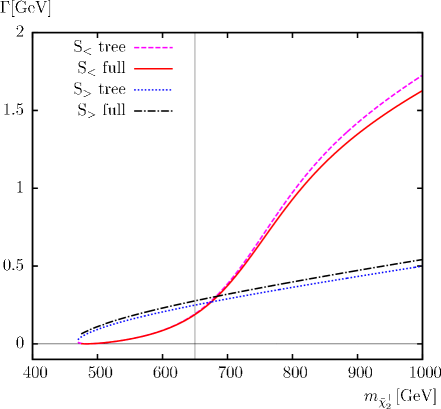
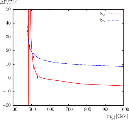
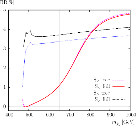
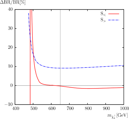
Figure 7: $\Gamma(\tilde{\chi}^{-}_{2}\to\tilde{\chi}^{0}_{1}H^{-})$. Tree-level (“tree”) and full one-loop (“full”) corrected decay widths are shown with the parameters chosen according to ${\cal S}$ (see Tab. 1), with $m_{\tilde{\chi}^{\pm}_{2}}$ varied. The upper left plot shows the decay width, the upper right plot shows the relative size of the corrections. The lower left plot shows the BR, the lower right plot shows the relative size of the BR. The vertical lines indicate where $m_{\tilde{\chi}^{\pm}_{1}}+m_{\tilde{\chi}^{\pm}_{2}}=1000\,\,\mathrm{GeV}$, i.e. the maximum reach of the ILC(1000).

We start our numerical analysis with the decays $\tilde{\chi}^{-}_{2}\to\tilde{\chi}^{0}_{i}H^{-}$ ($i=1,2,3$, where $\tilde{\chi}^{-}_{2}\to\tilde{\chi}^{0}_{4}H^{-}$ is kinematically forbidden). The results for $\tilde{\chi}^{-}_{2}\to\tilde{\chi}^{0}_{1}H^{-}$ are presented in Fig. 7. The dips, visible best in the upper right plots are due to thresholds in the vertex corrections. At $m_{\tilde{\chi}^{\pm}_{2}}=488\,\,\mathrm{GeV}$ the $\tilde{\chi}^{\pm}_{1}h_{2}$ threshold can be seen in ${\cal S}_{>}$ (with the $\tilde{\chi}^{\pm}_{1}h_{3}$ threshold only $\sim 0.5\,\,\mathrm{GeV}$ above remains nearly invisible). A second dip can be seen at $m_{\tilde{\chi}^{\pm}_{2}}=510\ (513)\,\,\mathrm{GeV}$ in ${\cal S}_{>}$ (${\cal S}_{<}$) corresponding to the $\tilde{\chi}^{0}_{2}H^{-}$ threshold, and a third dip in ${\cal S}_{<}$ at $m_{\tilde{\chi}^{\pm}_{2}}=533\,\,\mathrm{GeV}$ corresponding to the $\tilde{\chi}^{0}_{3}H^{-}$ threshold. In ${\cal S}_{>}$ and ${\cal S}_{<}$ for low $m_{\tilde{\chi}^{\pm}_{2}}$ the higgsino component of the heavy chargino allows the decay to the bino-like $\tilde{\chi}^{0}_{1}$ and the charged Higgs. At large $m_{\tilde{\chi}^{\pm}_{2}}$ within ${\cal S}_{<}$ the lightest neutralino changes from bino to wino dominated and the decay proceeds via the “fully allowed” higgsino-wino interaction with a corresponding increase in the decay width. Within ${\cal S}_{>}$, on the other hand, we find a pure higgsino-bino induced decay. The loop corrections can be larger than $20\%$ at the smallest $m_{\tilde{\chi}^{\pm}_{2}}$ in both scenarios, see the discussion in Sect. 2.3 on the $\mu\simeq M_{2}$ region. At large $m_{\tilde{\chi}^{\pm}_{2}}$ the size of the loop corrections levels out at $\sim-6\%\ (+9\%)$ in ${\cal S}_{<}$ (${\cal S}_{>}$). The BR in ${\cal S}_{<}$ rises from zero at $m_{\tilde{\chi}^{\pm}_{2}}\simeq 485\,\,\mathrm{GeV}$ to above $4.5\%$, whereas in ${\cal S}_{>}$ it is found around $4\%$ for most of the parameter space. The corrections to the BR’s reach the level of $30\%$ at the smallest $m_{\tilde{\chi}^{\pm}_{2}}$. In ${\cal S}_{>}$ they are found to be around $\sim-1\%$ for $m_{\tilde{\chi}^{\pm}_{2}}\;\raisebox{-3.00003pt}{$\stackrel{{\scriptstyle\displaystyle>}}{{\sim}}$}\;600\,\,\mathrm{GeV}$, whereas in ${\cal S}_{<}$ they remain at the $10\%$ level. In view of the ILC precision at the per-cent level, at least in ${\cal S}_{<}$ the loop corrections are highly relevant.

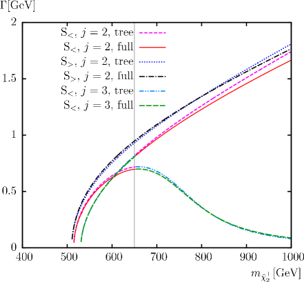
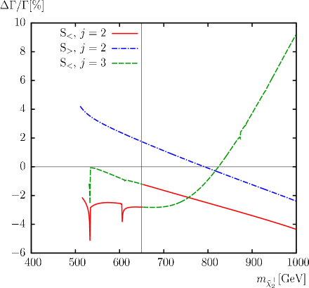
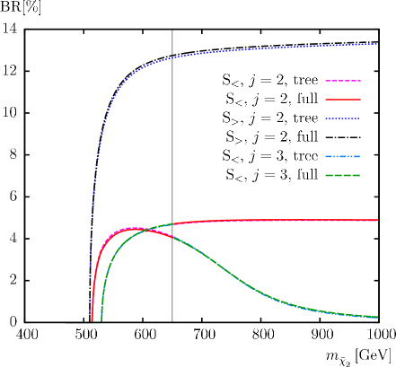
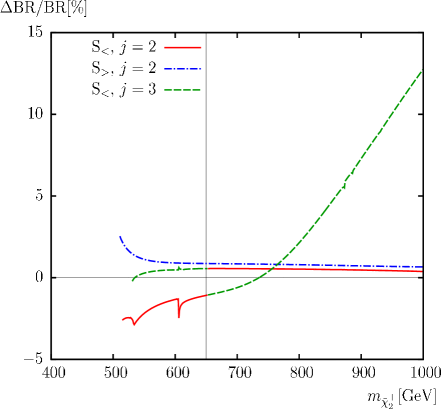
Figure 8: $\Gamma(\tilde{\chi}^{-}_{2}\to\tilde{\chi}^{0}_{j}H^{-})$ for $j=2,3$. Tree-level (“tree”) and full one-loop (“full”) corrected decay widths are shown with the parameters chosen according to ${\cal S}$ (see Tab. 1), with $m_{\tilde{\chi}^{\pm}_{2}}$ varied. The upper left plot shows the decay width, the upper right plot shows the relative size of the corrections. The lower left plot shows the BR, the lower right plot shows the relative size of the BR. The vertical lines indicate where $m_{\tilde{\chi}^{\pm}_{1}}+m_{\tilde{\chi}^{\pm}_{2}}=1000\,\,\mathrm{GeV}$, i.e. the maximum reach of the ILC(1000).

The results for $\tilde{\chi}^{-}_{2}\to\tilde{\chi}^{0}_{j}H^{-}$ ($j=2,3$) are shown in Fig. 8. The dip in ${\cal S}_{<}$ at $m_{\tilde{\chi}^{\pm}_{2}}=533\,\,\mathrm{GeV}$ visible in $\tilde{\chi}^{-}_{2}\to\tilde{\chi}^{0}_{2}H^{-}$ stems from the $\tilde{\chi}^{0}_{3}H^{-}$ threshold. Finally dips in $\tilde{\chi}^{-}_{2}\to\tilde{\chi}^{0}_{2(3)}H^{-}$ can be observed at $m_{\tilde{\chi}^{\pm}_{2}}\sim 604,606,(873,886)\,\,\mathrm{GeV}$, which correspond, respectively, to the thresholds $\tilde{\chi}^{0}_{2}\to\tilde{\chi}^{0}_{1}Z$, $\tilde{\chi}^{0}_{2}\to\tilde{\chi}^{0}_{1}h$ ($\tilde{\chi}^{0}_{3}\to\tilde{\chi}^{0}_{1}h$, $\tilde{\chi}^{0}_{3}\to\tilde{\chi}^{\pm}_{1}W^{\mp}$). As before the general behavior of the decay widths can be understood from the decomposition of the heavy chargino and the neutralinos. In ${\cal S}_{>}$ only the decay $\tilde{\chi}^{-}_{2}\to\tilde{\chi}^{0}_{2}H^{-}$ is kinematically allowed, and the width rises up to $\sim 1.7\,\,\mathrm{GeV}$ for large $m_{\tilde{\chi}^{\pm}_{2}}$. In ${\cal S}_{<}$ two observations can be made. At $m_{\tilde{\chi}^{\pm}_{2}}=652\,\,\mathrm{GeV}$ the $\tilde{\chi}^{0}_{2}$ and $\tilde{\chi}^{0}_{3}$ “switch character”. For this chargino mass one finds $m_{\tilde{\chi}^{0}_{2}}=m_{\tilde{\chi}^{0}_{3}}$, and the neutralino mixing matrix exhibits a discontinuity. As a consequence, as can be observed in Fig. 8, the $\tilde{\chi}^{0}_{2}$-curves continue for $\tilde{\chi}^{0}_{3}$ and vice versa. At low masses we find “partially” allowed wino/higgsino interaction for $\tilde{\chi}^{-}_{2}\to\tilde{\chi}^{0}_{2,3}H^{-}$. At high masses the $\tilde{\chi}^{0}_{2}$ couples as a higgsino to the charged wino, whereas the $\tilde{\chi}^{0}_{3}$ becomes a bino and decouples from the wino-like $\tilde{\chi}^{\pm}_{2}$, and the decay width goes to zero. The relative size of the one-loop corrections to the decay width vary roughly between $-4\%$ and $+4\%$. The ${\rm BR}(\tilde{\chi}^{-}_{2}\to\tilde{\chi}^{0}_{2}H^{-})$ in ${\cal S}_{>}$ reaches $\sim 12\%$ already close to threshold, whereas in ${\cal S}_{<}$ it rises only up to $\sim 5\%$ due to the larger total width, see below. The ${\rm BR}(\tilde{\chi}^{-}_{2}\to\tilde{\chi}^{0}_{3}H^{-})$ in ${\cal S}_{<}$ reaches a maximum of $4\%$ around $m_{\tilde{\chi}^{\pm}_{2}}\approx 600\,\,\mathrm{GeV}$ and goes to zero for larger chargino masses. The relative size of the one-loop effects on the BR’s remains below $3\%$ in the ILC(1000) relevant mass region, which, however, can still be relevant, see Tab. 4.

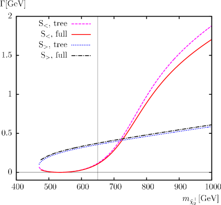
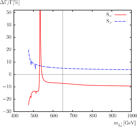
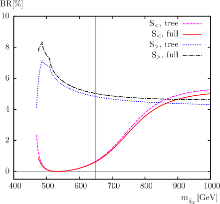
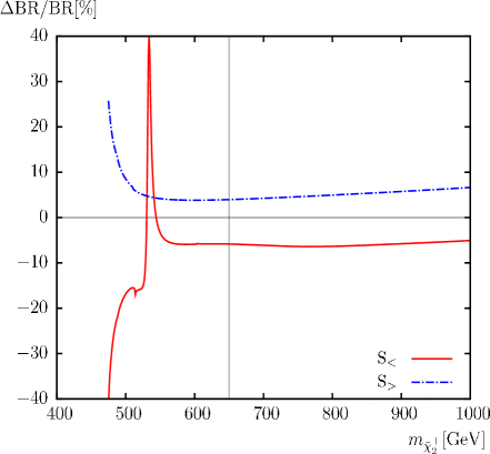
Figure 9: $\Gamma(\tilde{\chi}^{-}_{2}\to\tilde{\chi}^{0}_{1}W^{-})$. Tree-level (“tree”) and full one-loop (“full”) corrected decay widths are shown with the parameters chosen according to ${\cal S}$ (see Tab. 2), with $m_{\tilde{\chi}^{\pm}_{2}}$ varied. The upper left plot shows the decay width, the upper right plot shows the relative size of the corrections. The lower left plot shows the BR, the lower right plot shows the relative size of the BR. The vertical lines indicate where $m_{\tilde{\chi}^{\pm}_{1}}+m_{\tilde{\chi}^{\pm}_{2}}=1000\,\,\mathrm{GeV}$, i.e. the maximum reach of the ILC(1000).

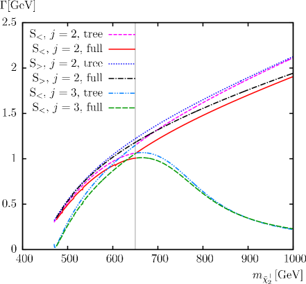
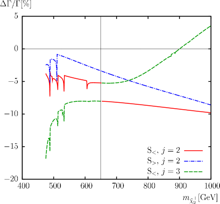
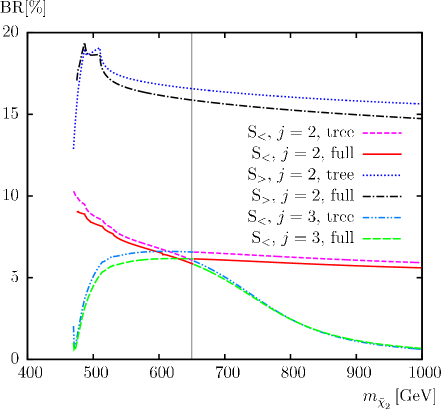
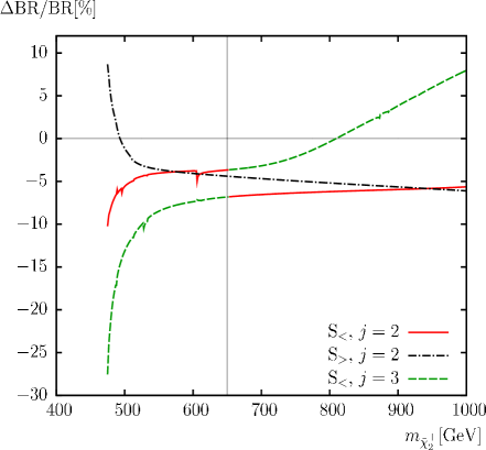
Figure 10: $\Gamma(\tilde{\chi}^{-}_{2}\to\tilde{\chi}^{0}_{j}W^{-})$ for $j=2,3$. Tree-level (“tree”) and full one-loop (“full”) corrected decay widths are shown with the parameters chosen according to ${\cal S}$ (see Tab. 1), with $m_{\tilde{\chi}^{\pm}_{2}}$ varied. The upper left plot shows the decay width, the upper right plot shows the relative size of the corrections. The lower left plot shows the BR, the lower right plot shows the relative size of the BR. The vertical lines indicate where $m_{\tilde{\chi}^{\pm}_{1}}+m_{\tilde{\chi}^{\pm}_{2}}=1000\,\,\mathrm{GeV}$, i.e. the maximum reach of the ILC(1000).

Next we analyze the decays $\tilde{\chi}^{-}_{2}\to\tilde{\chi}^{0}_{1,2,3}W^{-}$ shown in Figs. 9, 10. The general behavior of the decays to $W^{-}$ is very similar to the decays to $H^{-}$ discussed above. The lightest neutralino is presented in Fig. 9. The dip at $m_{\tilde{\chi}^{\pm}_{2}}=488\,\,\mathrm{GeV}$ corresponds to the $\tilde{\chi}^{\pm}_{1}h_{2}$ threshold. A second dip can be seen at $m_{\tilde{\chi}^{\pm}_{2}}=510\ (513)\,\,\mathrm{GeV}$ in ${\cal S}_{>}$ (${\cal S}_{<}$) to the $\tilde{\chi}^{0}_{2}H^{-}$ threshold, as in $\tilde{\chi}^{-}_{2}\to\tilde{\chi}^{0}_{1}H^{-}$, and a third dip at $m_{\tilde{\chi}^{\pm}_{2}}=533\,\,\mathrm{GeV}$ in ${\cal S}_{<}$. The size of the decay widths for the decay $\tilde{\chi}^{-}_{2}\to\tilde{\chi}^{0}_{1}W^{-}$ can be understood as follows. The dominant components of $\tilde{\chi}^{\pm}_{2}$ and $\tilde{\chi}^{0}_{1}$ have a vanishing coupling according to Eq. (111). The size of the width is then driven by the “small” components with a generic size of $\sim M_{W}/M_{2}$. However, their smallness is compensated by factors of $M_{2}/M_{W}$, as can be seen in the tree-level expression, Eq. (3). In ${\cal S}_{>}$ the width rises from $0.1\,\,\mathrm{GeV}$ at the lowest $m_{\tilde{\chi}^{\pm}_{2}}$ up to $\sim 0.6\,\,\mathrm{GeV}$ at high $m_{\tilde{\chi}^{\pm}_{2}}$ values. In ${\cal S}_{<}$ we find a minimum (reaching zero) around $m_{\tilde{\chi}^{\pm}_{2}}=540\,\,\mathrm{GeV}$, and rising up to $\sim 1.6\,\,\mathrm{GeV}$ including one-loop corrections. The relative size of the corrections varies between $\sim+10\%$ and $+4\%$ in ${\cal S}_{>}$ and around $-10\%$ in ${\cal S}_{<}$ (apart from the region where the width is negligible small). The BR’s behave accordingly, reaching $\sim 8\%$ in ${\cal S}_{>}$ for $m_{\tilde{\chi}^{\pm}_{2}}\approx 500\,\,\mathrm{GeV}$, going down to $\sim 4.5\,\,\mathrm{GeV}$ for large $m_{\tilde{\chi}^{\pm}_{2}}$, where in ${\cal S}_{<}$ values up to $5\%$ are found. The relative size of the one-loop effects on the BR’s in the ILC(1000) relevant mass region varies between $+10\%$ and $+3\%$ in ${\cal S}_{>}$ and between $\sim-20\%$ and $-7\%$ in ${\cal S}_{<}$. This corresponds to several times the anticipated ILC(1000) precision.

The decays involving the heavier neutralinos, $\tilde{\chi}^{-}_{2}\to\tilde{\chi}^{0}_{2,3}W^{-}$ (where the decay $\tilde{\chi}^{-}_{2}\to\tilde{\chi}^{0}_{4}W^{-}$ is kinematically forbidden) are presented in Fig. 10. The two dips in ${\cal S}_{>}$ for $\tilde{\chi}^{-}_{2}\to\tilde{\chi}^{0}_{2}W^{-}$ stem from the $\tilde{\chi}^{\pm}_{1}h_{2}$ and the $\tilde{\chi}^{0}_{2}H^{-}$ threshold, which can also be observed in the two other curves in ${\cal S}_{<}$. In ${\cal S}_{<}$ an additional dip from the $\tilde{\chi}^{0}_{3}H^{-}$ threshold can be seen at $m_{\tilde{\chi}^{\pm}_{2}}=533\,\,\mathrm{GeV}$ for $\tilde{\chi}^{-}_{2}\to\tilde{\chi}^{0}_{2,3}W^{-}$. Finally the dips at $m_{\tilde{\chi}^{\pm}_{2}}\sim 604,606,873,886\,\,\mathrm{GeV}$ have been described for $\tilde{\chi}^{-}_{2}\to\tilde{\chi}^{0}_{2,3}H^{-}$. The behavior of the decays $\tilde{\chi}^{-}_{2}\to\tilde{\chi}^{0}_{2,3}W^{-}$, as stated above, is similar to the one of $\tilde{\chi}^{-}_{2}\to\tilde{\chi}^{0}_{2,3}H^{-}$, where again the small chargino/neutralino components determine the size of the widths. As for $\tilde{\chi}^{-}_{2}\to\tilde{\chi}^{0}_{1}H^{-}$ the smallness of the components is compensated by factors $\sim M_{2}/M_{W}$ in the tree-level expressions, see Eq. (3). Also the “character switch” between $\tilde{\chi}^{0}_{2}$ and $\tilde{\chi}^{0}_{3}$ in ${\cal S}_{<}$ appears as in Fig. 8. The relative size of the one-loop corrections, shown in the upper right plot, are found around $\sim-10\%$ and $\sim-5\%$ in ${\cal S}_{<}$, except where the width becomes very small. In ${\cal S}_{>}$ the one-loop corrections are small close to threshold and grow to $\sim-9\%$ at large $m_{\tilde{\chi}^{\pm}_{2}}$. The ${\rm BR}(\tilde{\chi}^{-}_{2}\to\tilde{\chi}^{0}_{2}W^{-})$ in ${\cal S}_{>}$ reaches a maximum of $19\%$ around $m_{\tilde{\chi}^{\pm}_{2}}=500\,\,\mathrm{GeV}$ and settles at $\sim 15\%$ at large $m_{\tilde{\chi}^{\pm}_{2}}$. In ${\cal S}_{<}$ the BR’s are between $\sim 5\%$ and $10\%$ in the ILC(1000) relevant region, where $\sim 5\%$ are also found for ${\rm BR}(\tilde{\chi}^{-}_{2}\to\tilde{\chi}^{0}_{2}W^{-})$ for large $m_{\tilde{\chi}^{\pm}_{2}}$. The relative size of the one-loop effects on the BR’s in the ILC(1000) region (and not directly at the production threshold) is found between $\sim-10\%$ and $\sim-5\%$. Again, this corresponds to several times the anticipated ILC(1000) precision.

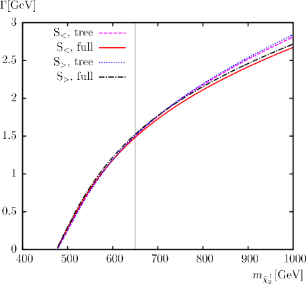
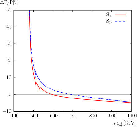
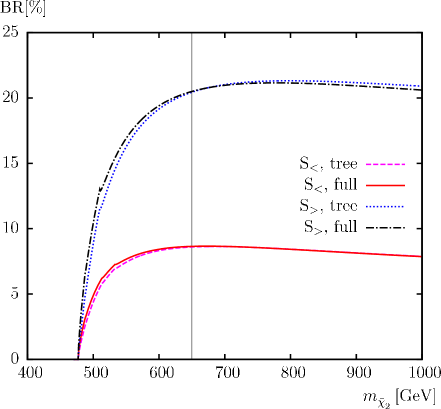
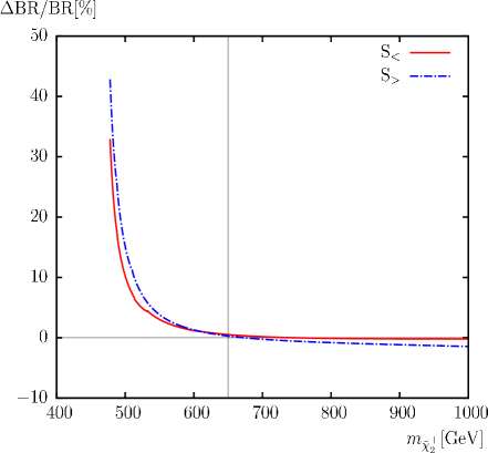
Figure 11: $\Gamma(\tilde{\chi}^{-}_{2}\to\tilde{\chi}^{-}_{1}h_{1})$. Tree-level (“tree”) and full one-loop (“full”) corrected decay widths are shown with the parameters chosen according to ${\cal S}$ (see Tab. 1), with $m_{\tilde{\chi}^{\pm}_{2}}$ varied. The upper left plot shows the decay width, the upper right plot shows the relative size of the corrections. The lower left plot shows the BR, the lower right plot shows the relative size of the BR. The vertical lines indicate where $m_{\tilde{\chi}^{\pm}_{1}}+m_{\tilde{\chi}^{\pm}_{2}}=1000\,\,\mathrm{GeV}$, i.e. the maximum reach of the ILC(1000).

Now we turn to the decays involving neutral Higgs bosons. The channels $\tilde{\chi}^{-}_{2}\to\tilde{\chi}^{-}_{1}h_{k}$ ($k=1,2,3$) can serve as source for Higgs production from SUSY cascades at the LHC, and are therefore of particular interest. The decay $\tilde{\chi}^{-}_{2}\to\tilde{\chi}^{-}_{1}h_{1}$ is shown in Fig. 11. The dips are due to the $\tilde{\chi}^{\pm}_{1}h_{2}$, $\tilde{\chi}^{0}_{2}H^{-}$ and $\tilde{\chi}^{0}_{3}H^{-}$ thresholds and have been described in $\tilde{\chi}^{-}_{2}\to\tilde{\chi}^{0}_{2,3}W^{-}$, see above. The tree-level results show a very small difference between ${\cal S}_{>}$ and ${\cal S}_{<}$. This holds also after the full one-loop corrections are included. The widths rise from zero at threshold to $\sim 2.6\,\,\mathrm{GeV}$. The soft rise at threshold is due to the p-wave suppression of the decay into a ${\cal CP}$-even scalar. As for the decays to a charged Higgs boson the admixture of the charginos is crucial for the size of the decay widths: from the wino/higgsino mixtures at low $m_{\tilde{\chi}^{\pm}_{2}}$ nearly pure wino and higgsino states are reached at large $m_{\tilde{\chi}^{\pm}_{2}}$, corresponding to an “allowed” coupling in Eq. (114). The size of the one-loop corrections slightly above the production threshold is relatively large, $\;\raisebox{-3.00003pt}{$\stackrel{{\scriptstyle\displaystyle>}}{{\sim}}$}\;+10\%$, and dominated by their s-wave contribution, and reaches $\sim-5\%$ at large $m_{\tilde{\chi}^{\pm}_{2}}$. The BR’s reach $20\%$ in ${\cal S}_{>}$ and $9\%$ in ${\cal S}_{<}$ at the highest $m_{\tilde{\chi}^{\pm}_{2}}$ values in the ILC(1000) relevant region, and remain nearly flat for higher $m_{\tilde{\chi}^{\pm}_{2}}$ values. The relative size of the one-loop effects on the BR’s is only sizable close to threshold, and is found at the $\sim 1\%$ level for $m_{\tilde{\chi}^{\pm}_{2}}\;\raisebox{-3.00003pt}{$\stackrel{{\scriptstyle\displaystyle>}}{{\sim}}$}\;600\,\,\mathrm{GeV}$, which corresponds roughly to the anticipated ILC(1000) precision, see Tab. 4.

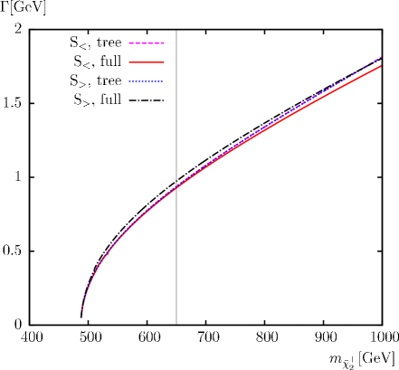
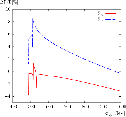
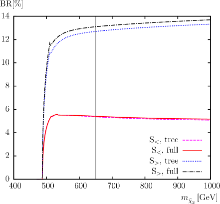
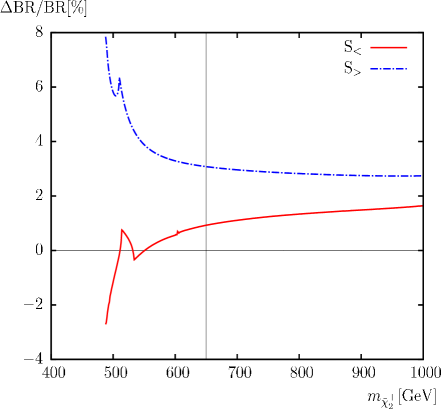
Figure 12: $\Gamma(\tilde{\chi}^{-}_{2}\to\tilde{\chi}^{-}_{1}h_{2})$. Tree-level (“tree”) and full one-loop (“full”) corrected decay widths are shown with the parameters chosen according to ${\cal S}$ (see Tab. 1), with $m_{\tilde{\chi}^{\pm}_{2}}$ varied. The upper left plot shows the decay width, the upper right plot shows the relative size of the corrections. The lower left plot shows the BR, the lower right plot shows the relative size of the BR. The vertical lines indicate where $m_{\tilde{\chi}^{\pm}_{1}}+m_{\tilde{\chi}^{\pm}_{2}}=1000\,\,\mathrm{GeV}$, i.e. the maximum reach of the ILC(1000).

The decay $\tilde{\chi}^{-}_{2}\to\tilde{\chi}^{-}_{1}h_{2}$ are shown in Fig. 12, where a qualitatively similar result to $\tilde{\chi}^{-}_{2}\to\tilde{\chi}^{-}_{1}h_{1}$ can be found, with the main difference of somewhat smaller decay width and branching ratio, mostly due to the smaller and negative contribution of the chirally violating part in the corresponding coupling, see Eq. (3). The steep rise at threshold is due to the unsuppressed s-wave contribution of this channel, where $h_{2}$ is the ${\cal CP}$-odd Higgs boson. The dips at $m_{\tilde{\chi}^{\pm}_{2}}=510\,\,\mathrm{GeV}$ in ${\cal S}_{>}$ and $m_{\tilde{\chi}^{\pm}_{2}}=513,533\,\,\mathrm{GeV}$ correspond to the thresholds described above for $\tilde{\chi}^{-}_{2}\to\tilde{\chi}^{-}_{1}h_{1}$. Finally, the dip at $m_{\tilde{\chi}^{\pm}_{2}}=606\,\,\mathrm{GeV}$ corresponds to the $\tilde{\chi}^{-}_{1}\to\tilde{\chi}^{0}_{1}W^{-}$ threshold. It should be noticed that the dips correspond to the thresholds for tree-level processes while the widths are evaluated with one-loop masses, leading to the effect of the $\tilde{\chi}^{\pm}_{1}h_{2}$ threshold in this decay, (see, however, footnote 8). The relative size of the one-loop corrections on the decay width varies in ${\cal S}_{<}$ between $+8\%$ at $m_{\tilde{\chi}^{\pm}_{2}}=500\,\,\mathrm{GeV}$ and very small negative values for large $m_{\tilde{\chi}^{\pm}_{2}}$ (where possible larger negative values can be reached for even larger $m_{\tilde{\chi}^{\pm}_{2}}$). In ${\cal S}_{<}$ the corrections vary around $\sim-3\%$. Concerning the one-loop effects on the BR’s, in ${\cal S}_{>}$ at $m_{\tilde{\chi}^{\pm}_{2}}=500\,\,\mathrm{GeV}$ around $+6\%$ are found, going down to $\sim+3\%$ at large $m_{\tilde{\chi}^{\pm}_{2}}$. In ${\cal S}_{<}$ the corrections vary between $-2\%$ at low $m_{\tilde{\chi}^{\pm}_{2}}$ and $+2\%$ at high $m_{\tilde{\chi}^{\pm}_{2}}$. For small $m_{\tilde{\chi}^{\pm}_{2}}$ values the corrections can be substantially larger than the ILC(1000) precision.

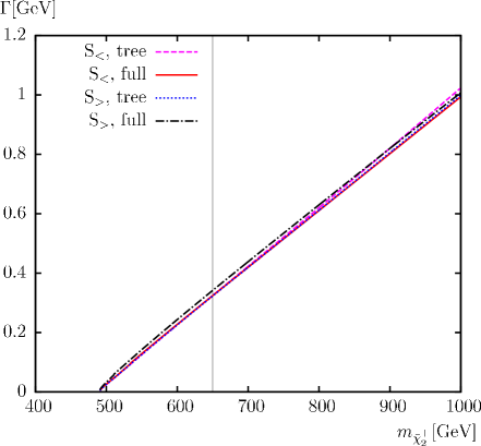
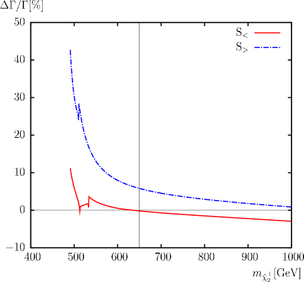
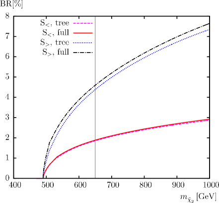
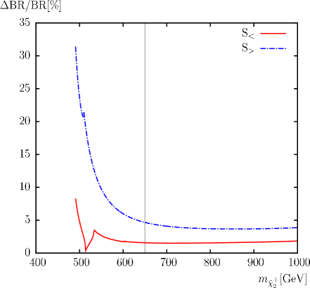
Figure 13: $\Gamma(\tilde{\chi}^{-}_{2}\to\tilde{\chi}^{-}_{1}h_{3})$. Tree-level (“tree”) and full one-loop (“full”) corrected decay widths are shown with the parameters chosen according to ${\cal S}$ (see Tab. 1), with $m_{\tilde{\chi}^{\pm}_{2}}$ varied. The upper left plot shows the decay width, the upper right plot shows the relative size of the corrections. The lower left plot shows the BR, the lower right plot shows the relative size of the BR. The vertical lines indicate where $m_{\tilde{\chi}^{\pm}_{1}}+m_{\tilde{\chi}^{\pm}_{2}}=1000\,\,\mathrm{GeV}$, i.e. the maximum reach of the ILC(1000).

The last channel involving a neutral Higgs, $\tilde{\chi}^{-}_{2}\to\tilde{\chi}^{-}_{1}h_{3}$ is shown in Fig. 13. We observe the same dips as for $\tilde{\chi}^{-}_{2}\to\tilde{\chi}^{-}_{1}h_{2}$. A straight rise of the decay width in ${\cal S}_{>}$ and ${\cal S}_{<}$ is found, reaching $\sim 1\,\,\mathrm{GeV}$ at $m_{\tilde{\chi}^{\pm}_{2}}=1000\,\,\mathrm{GeV}$. The smaller results with respect to $\tilde{\chi}^{-}_{2}\to\tilde{\chi}^{-}_{1}h_{1}$ are due to the opposite sign of the chirally violating contributions in the corresponding coupling, see Eq. (3). As in the decay into $h_{1}$, the threshold behavior is p-wave suppressed at tree-level with a small s-wave dominated contribution to the loop corrections. A corresponding rise in the BR up to $7.5\%$ ($3\%$) is found in ${\cal S}_{>}$ (${\cal S}_{<}$). Within ${\cal S}_{>}$ the relative size of the one-loop corrections is small above threshold, reaching $\sim-5\%$ at large $m_{\tilde{\chi}^{\pm}_{2}}$. Within ${\cal S}_{<}$ the corrections can be very large slightly above threshold, reaching $\sim 30\%$ at $m_{\tilde{\chi}^{\pm}_{2}}\;\raisebox{-3.00003pt}{$\stackrel{{\scriptstyle\displaystyle>}}{{\sim}}$}\;500\,\,\mathrm{GeV}$, going down to zero for large $m_{\tilde{\chi}^{\pm}_{2}}$. The relative effect on the BR’s is similar, where values around $5\%$–$10\%$ ($\sim 2.5\%$) are found in ${\cal S}_{>}$ (${\cal S}_{<}$), exceeding by far the anticipated ILC(1000) precision.

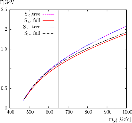
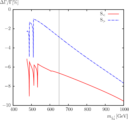
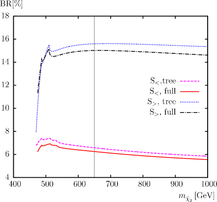
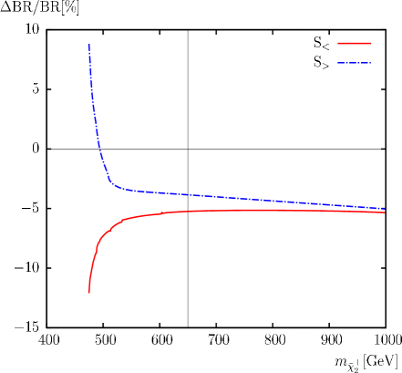
Figure 14: $\Gamma(\tilde{\chi}^{-}_{2}\to\tilde{\chi}^{-}_{1}Z)$. Tree-level (“tree”) and full one-loop (“full”) corrected decay widths are shown with the parameters chosen according to ${\cal S}$ (see Tab. 1), with $m_{\tilde{\chi}^{\pm}_{2}}$ varied. The upper left plot shows the decay width, the upper right plot shows the relative size of the corrections. The lower left plot shows the BR, the lower right plot shows the relative size of the BR. The vertical lines indicate where $m_{\tilde{\chi}^{\pm}_{1}}+m_{\tilde{\chi}^{\pm}_{2}}=1000\,\,\mathrm{GeV}$, i.e. the maximum reach of the ILC(1000).

The last channel involving SM gauge bosons, $\tilde{\chi}^{-}_{2}\to\tilde{\chi}^{-}_{1}Z$, is presented in Fig. 14. The same dips as in the decays into neutral Higgs bosons can be observed. The tree-level widths are equal in the two scenarios ${\cal S}_{>}$ and ${\cal S}_{<}$, since both the $Z\tilde{\chi}^{\pm}_{1}\tilde{\chi}^{\pm}_{2}$ coupling as well as the two chargino masses are symmetric under the exchange of $\mu\leftrightarrow M_{2}$. As for the decays $\tilde{\chi}^{-}_{2}\to\tilde{\chi}^{0}_{1,2,3}W^{-}$ the large admixtures of the charginos yield mostly a vanishing decay width. However, as above, the smallness of the “allowed couplings” is compensated by factors in the tree-level expression $\sim M_{2}/M_{Z}$, see Eq. (3). Including one-loop corrections the decay widths rise up to $\sim 1.9\,\,\mathrm{GeV}$ for $m_{\tilde{\chi}^{\pm}_{2}}=1000\,\,\mathrm{GeV}$, where, contrary to the tree-level widths, a small difference between ${\cal S}_{>}$ and ${\cal S}_{<}$ can be observed. The branching ratios are, except at the smallest $m_{\tilde{\chi}^{\pm}_{2}}$, relatively flat around $14.5\%$ $(6\%)$ in ${\cal S}_{>}$ (${\cal S}_{<}$). The size of the one-loop corrections to the decay width grows from $\sim-2\%$ $(-6\%)$ at small $m_{\tilde{\chi}^{\pm}_{2}}$ to $-7.5\%$ $(-9.5\%)$ at large $m_{\tilde{\chi}^{\pm}_{2}}$ in ${\cal S}_{>}$ (${\cal S}_{<}$). The effects on the branching ratios is mostly at the $-5\%$ level, which is larger than the ILC(1000) precision.

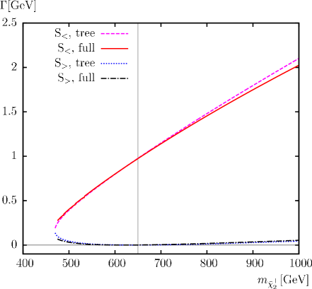
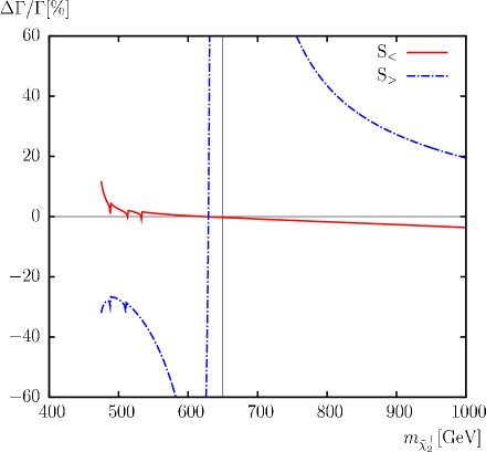
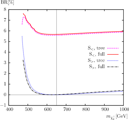
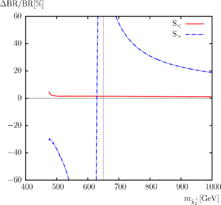
Figure 15: $\Gamma(\tilde{\chi}^{-}_{2}\to\bar{\nu}_{\tau}\,\tilde{\tau}_{1}^{-})$. Tree-level (“tree”) and full one-loop (“full”) corrected decay widths are shown with the parameters chosen according to ${\cal S}$ (see Tab. 1), with $m_{\tilde{\chi}^{\pm}_{2}}$ varied. The upper left plot shows the decay width, the upper right plot shows the relative size of the corrections. The lower left plot shows the BR, the lower right plot shows the relative size of the BR. The vertical lines indicate where $m_{\tilde{\chi}^{\pm}_{1}}+m_{\tilde{\chi}^{\pm}_{2}}=1000\,\,\mathrm{GeV}$, i.e. the maximum reach of the ILC(1000).

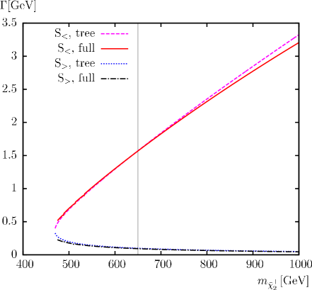
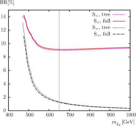
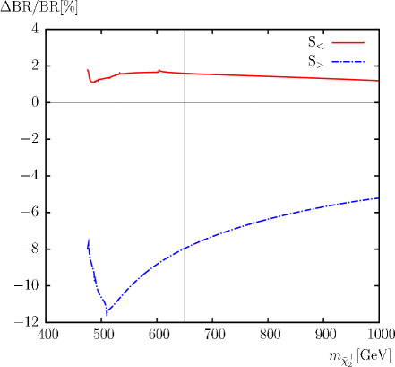
Figure 17: $\Gamma(\tilde{\chi}^{-}_{2}\to\bar{\nu}_{\mu}\,\tilde{\mu}_{1}^{-})$. Tree-level (“tree”) and full one-loop (“full”) corrected decay widths are shown with the parameters chosen according to ${\cal S}$ (see Tab. 1), with $m_{\tilde{\chi}^{\pm}_{2}}$ varied. The upper left plot shows the decay width, the upper right plot shows the relative size of the corrections. The lower left plot shows the BR, the lower right plot shows the relative size of the BR. The vertical lines indicate where $m_{\tilde{\chi}^{\pm}_{1}}+m_{\tilde{\chi}^{\pm}_{2}}=1000\,\,\mathrm{GeV}$, i.e. the maximum reach of the ILC(1000).

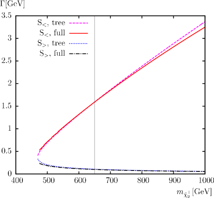
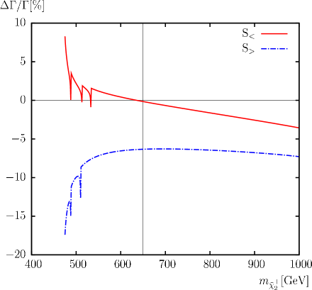
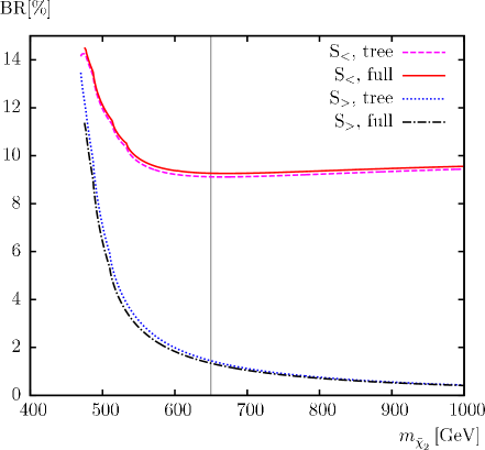
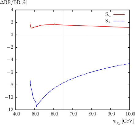
Figure 19: $\Gamma(\tilde{\chi}^{-}_{2}\to\bar{\nu}_{e}\,\tilde{e}_{1}^{-})$. Tree-level (“tree”) and full one-loop (“full”) corrected decay widths are shown with the parameters chosen according to ${\cal S}$ (see Tab. 1), with $m_{\tilde{\chi}^{\pm}_{2}}$ varied. The upper left plot shows the decay width, the upper right plot shows the relative size of the corrections. The lower left plot shows the BR, the lower right plot shows the relative size of the BR. The vertical lines indicate where $m_{\tilde{\chi}^{\pm}_{1}}+m_{\tilde{\chi}^{\pm}_{2}}=1000\,\,\mathrm{GeV}$, i.e. the maximum reach of the ILC(1000).

Now we turn to the decays involving (scalar) leptons. All these decay widths follow the same pattern that can be understood from Eqs. (115), (116). We have chosen $M_{\tilde{l}_{L}}<M_{\tilde{l}_{R}}$, leading to a left-handed lighter and a right-handed heavier slepton, where significant mixing can be found in the scalar tau sector. In Figs. 15, 17, 19 we show the decays $\tilde{\chi}^{-}_{2}\to\bar{\nu}_{\tau}\,\tilde{\tau}_{1}^{-},\tilde{\chi}^{-}_{2}\to\bar{\nu}_{\mu}\,\tilde{\mu}_{1}^{-},\tilde{\chi}^{-}_{2}\to\bar{\nu}_{e}\,\tilde{e}_{1}^{-}$ respectively. The dips, best visible in the upper right panels, are due to the $\tilde{\chi}^{\pm}_{1}h_{2}$, $\tilde{\chi}^{0}_{2}H^{-}$ and $\tilde{\chi}^{0}_{3}H^{-}$ thresholds and have been already described for $\tilde{\chi}^{-}_{2}\to\tilde{\chi}^{0}_{2,3}W^{-}$. Within ${\cal S}_{>}$ the $\tilde{\chi}^{\pm}_{2}$ turns from a mixed higgsino/wino state at low $m_{\tilde{\chi}^{\pm}_{2}}$ to a pure higgsino state at large $m_{\tilde{\chi}^{\pm}_{2}}$ with a vanishing coupling to the left-handed slepton. Consequently, these widths are very small, and only in the case of $\tilde{\tau}_{1}$, due to the mixture between left- and right-handed states it does not go to zero for large $m_{\tilde{\chi}^{\pm}_{2}}$, but goes through zero at $m_{\tilde{\chi}^{\pm}_{2}}\approx 600\,\,\mathrm{GeV}$ due to a cancellation of the higgsino (suppressed by the Yukawa term) and the small gaugino contributions to the $\tilde{\chi}^{-}_{2}\nu_{\tau}\tilde{\tau}_{1}^{\dagger}$ coupling. In ${\cal S}_{<}$, on the other hand, $\tilde{\chi}^{\pm}_{2}$ changes from the mixed wino/higgsino state to a wino-like state at large $m_{\tilde{\chi}^{\pm}_{2}}$, and the EW coupling (which is flavor independent) dominates the decay to the left-handed sleptons, leading to a rise of the decay widths to $\sim 3.2\,\,\mathrm{GeV}$ in the case of $\tilde{\chi}^{-}_{2}\to\bar{\nu}_{\mu}\,\tilde{\mu}_{1}^{-},\tilde{\chi}^{-}_{2}\to\bar{\nu}_{e}\,\tilde{e}_{1}^{-}$ and a reduced value of $2\,\,\mathrm{GeV}$ for $\tilde{\chi}^{-}_{2}\to\bar{\nu}_{\tau}\,\tilde{\tau}_{1}^{-}$, again due to the mixing in the stau sector. The ${\rm BR}(\tilde{\chi}^{-}_{2}\to\bar{\nu}_{\tau}\,\tilde{\tau}_{1}^{-})$ in ${\cal S}_{>}$ is large only at the smallest $m_{\tilde{\chi}^{\pm}_{2}}$ and below $\sim 0.5\%$ for most $m_{\tilde{\chi}^{\pm}_{2}}$ values. For the first and second slepton generation we also find a monotonous decrease, although a bit weaker than for the $\tilde{\tau}_{1}$. Within ${\cal S}_{<}$ the ${\rm BR}(\tilde{\chi}^{-}_{2}\to\bar{\nu}_{\tau}\,\tilde{\tau}_{1}^{-})$ is mostly found at $\sim 6\%$, whereas ${\rm BR}(\tilde{\chi}^{-}_{2}\to\bar{\nu}_{\mu}\,\tilde{\mu}_{1}^{-})$ and ${\rm BR}(\tilde{\chi}^{-}_{2}\to\bar{\nu}_{e}\,\tilde{e}_{1}^{-})$ are somewhat larger, due to the absence of mixing, and reaches $\sim 9.5\%$. The size of the one-loop corrections to the decay widths and BR’s is only substantial where the decay widths are small, reaching nearly $-12\%$ at $m_{\tilde{\chi}^{\pm}_{2}}\approx 500\,\,\mathrm{GeV}$ in ${\cal S}_{>}$. In the case of a large BR, i.e. in ${\cal S}_{<}$, the corrections stay at the level of $\sim 1\%$, staying below the precision anticipated for the ILC(1000).

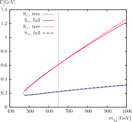
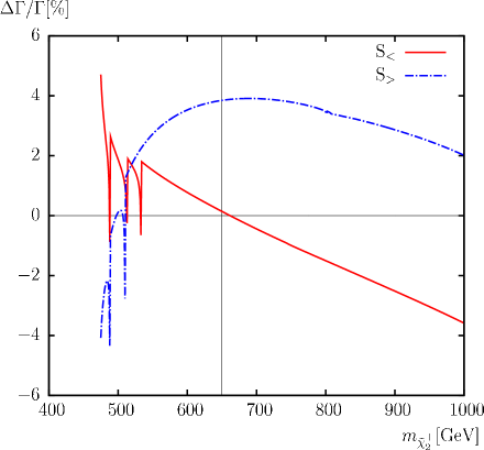
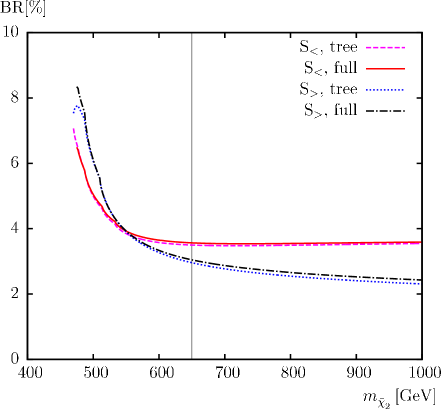
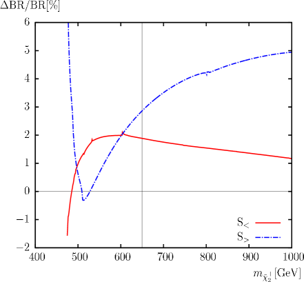
Figure 16: $\Gamma(\tilde{\chi}^{-}_{2}\to\bar{\nu}_{\tau}\,\tilde{\tau}_{2}^{-})$. Tree-level (“tree”) and full one-loop (“full”) corrected decay widths are shown with the parameters chosen according to ${\cal S}$ (see Tab. 1), with $m_{\tilde{\chi}^{\pm}_{2}}$ varied. The upper left plot shows the decay width, the upper right plot shows the relative size of the corrections. The lower left plot shows the BR, the lower right plot shows the relative size of the BR. The vertical lines indicate where $m_{\tilde{\chi}^{\pm}_{1}}+m_{\tilde{\chi}^{\pm}_{2}}=1000\,\,\mathrm{GeV}$, i.e. the maximum reach of the ILC(1000).

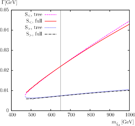
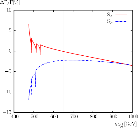
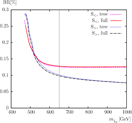
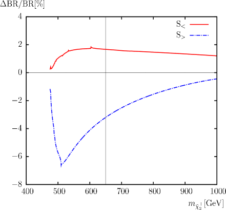
Figure 18: $\Gamma(\tilde{\chi}^{-}_{2}\to\bar{\nu}_{\mu}\,\tilde{\mu}_{2}^{-})$. Tree-level (“tree”) and full one-loop (“full”) corrected decay widths are shown with the parameters chosen according to ${\cal S}$ (see Tab. 1), with $m_{\tilde{\chi}^{\pm}_{2}}$ varied. The upper left plot shows the decay width, the upper right plot shows the relative size of the corrections. The lower left plot shows the BR, the lower right plot shows the relative size of the BR. The vertical lines indicate where $m_{\tilde{\chi}^{\pm}_{1}}+m_{\tilde{\chi}^{\pm}_{2}}=1000\,\,\mathrm{GeV}$, i.e. the maximum reach of the ILC(1000).

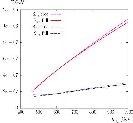
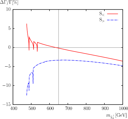
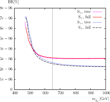
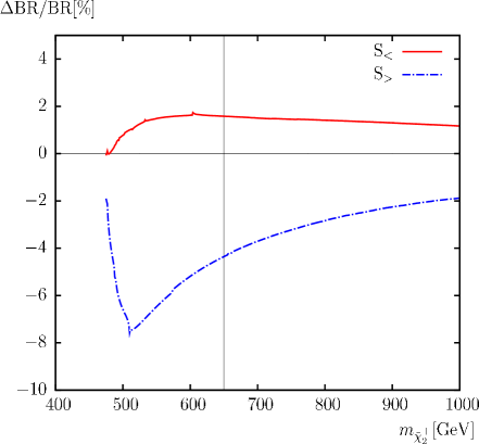
Figure 20: $\Gamma(\tilde{\chi}^{-}_{2}\to\bar{\nu}_{e}\,\tilde{e}_{2}^{-})$. Tree-level (“tree”) and full one-loop (“full”) corrected decay widths are shown with the parameters chosen according to ${\cal S}$ (see Tab. 1), with $m_{\tilde{\chi}^{\pm}_{2}}$ varied. The upper left plot shows the decay width, the upper right plot shows the relative size of the corrections. The lower left plot shows the BR, the lower right plot shows the relative size of the BR. The vertical lines indicate where $m_{\tilde{\chi}^{\pm}_{1}}+m_{\tilde{\chi}^{\pm}_{2}}=1000\,\,\mathrm{GeV}$, i.e. the maximum reach of the ILC(1000).

The decays to the heavier sleptons, $\tilde{\chi}^{-}_{2}\to\bar{\nu}_{\tau}\,\tilde{\tau}_{2}^{-},\tilde{\chi}^{-}_{2}\to\bar{\nu}_{\mu}\,\tilde{\mu}_{2}^{-},\tilde{\chi}^{-}_{2}\to\bar{\nu}_{e}\,\tilde{e}_{2}^{-}$, shown in Figs. 16, 18, 20, follow a similar pattern. The dips visible in the upper right panels stem from the same thresholds as those observed for the decays to the lighter sleptons. At low $m_{\tilde{\chi}^{\pm}_{2}}$ values the mixed higgsino/wino state couples to the right-handed sleptons through the Yukawa term $\propto m_{l}$. At large $m_{\tilde{\chi}^{\pm}_{2}}$ in ${\cal S}_{>}$ only the higgsino part of $\tilde{\chi}^{\pm}_{2}$ survives, leading to a (Yukawa term) suppressed coupling to the right-handed slepton and the corresponding decay widths are very small, below $0.3,0.01,2\times 10^{-7}\,\,\mathrm{GeV}$ for $\tilde{\chi}^{-}_{2}\to\bar{\nu}_{\tau}\,\tilde{\tau}_{2}^{-},\tilde{\chi}^{-}_{2}\to\bar{\nu}_{\mu}\,\tilde{\mu}_{2}^{-},\tilde{\chi}^{-}_{2}\to\bar{\nu}_{e}\,\tilde{e}_{2}^{-}$, respectively. In ${\cal S}_{<}$, on the other hand, the small wino component couples to the small left-handed admixture of the heavier slepton. For $\tilde{\chi}^{-}_{2}\to\bar{\nu}_{\tau}\,\tilde{\tau}_{2}^{-}$, due to the relatively large mixing, this still yields a loop-corrected decay width up to $1.2\,\,\mathrm{GeV}$ for large $m_{\tilde{\chi}^{\pm}_{2}}$, while for the first and second generation sleptons the widths stay below $0.045$ and $1.1\times 10^{-6}\,\,\mathrm{GeV}$, respectively. Substantial branching ratios are only found for $\tilde{\chi}^{-}_{2}\to\bar{\nu}_{\tau}\,\tilde{\tau}_{2}^{-}$, where values between $\sim 6\%$ and $\sim 2\%$ are realized. In this case the size of the one-loop corrections varies between $0$ and $+5\%$. At the high end, this exceeds the anticipated ILC(1000) accuracy.

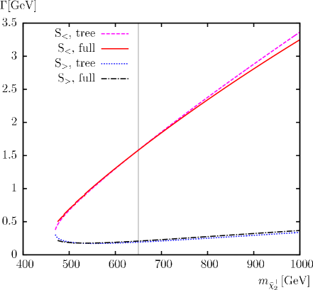
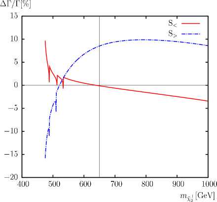
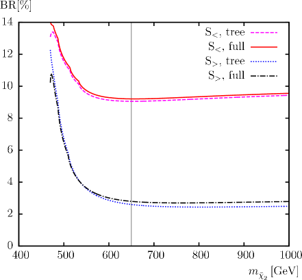
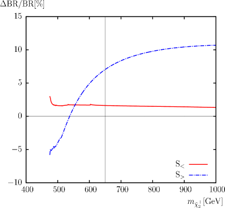
Figure 21: $\Gamma(\tilde{\chi}^{-}_{2}\to{\tau}^{-}\,\tilde{\nu}_{\tau}^{\dagger})$. Tree-level (“tree”) and full one-loop (“full”) corrected decay widths are shown with the parameters chosen according to ${\cal S}$ (see Tab. 1), with $m_{\tilde{\chi}^{\pm}_{2}}$ varied. The upper left plot shows the decay width, the upper right plot shows the relative size of the corrections. The lower left plot shows the BR, the lower right plot shows the relative size of the BR. The vertical lines indicate where $m_{\tilde{\chi}^{\pm}_{1}}+m_{\tilde{\chi}^{\pm}_{2}}=1000\,\,\mathrm{GeV}$, i.e. the maximum reach of the ILC(1000).

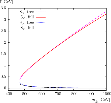
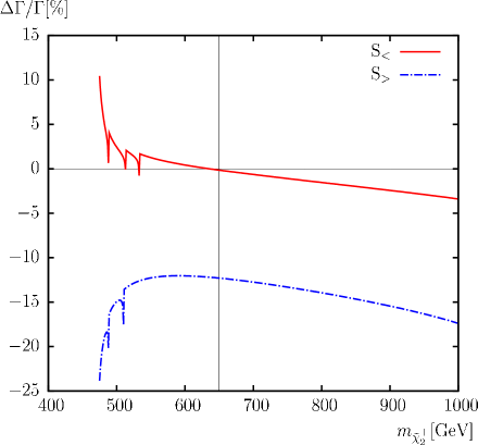
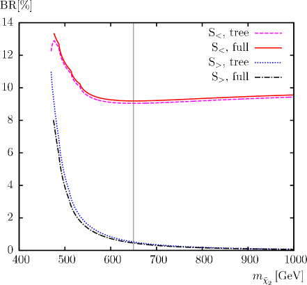
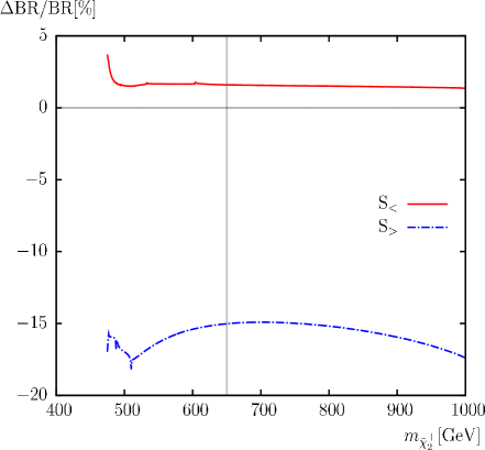
Figure 22: $\Gamma(\tilde{\chi}^{-}_{2}\to{\mu}^{-}\,\tilde{\nu}_{\mu}^{\dagger})$. Tree-level (“tree”) and full one-loop (“full”) corrected decay widths are shown with the parameters chosen according to ${\cal S}$ (see Tab. 1), with $m_{\tilde{\chi}^{\pm}_{2}}$ varied. The upper left plot shows the decay width, the upper right plot shows the relative size of the corrections. The lower left plot shows the BR, the lower right plot shows the relative size of the BR. The vertical lines indicate where $m_{\tilde{\chi}^{\pm}_{1}}+m_{\tilde{\chi}^{\pm}_{2}}=1000\,\,\mathrm{GeV}$, i.e. the maximum reach of the ILC(1000).

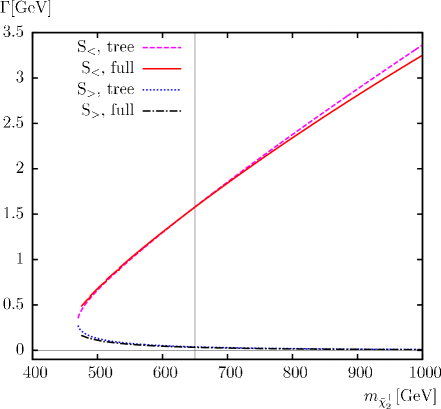
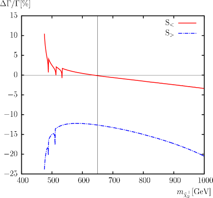
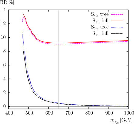
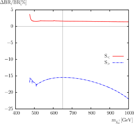
Figure 23: $\Gamma(\tilde{\chi}^{-}_{2}\to{e}^{-}\,\tilde{\nu}_{e}^{\dagger})$. Tree-level (“tree”) and full one-loop (“full”) corrected decay widths are shown with the parameters chosen according to ${\cal S}$ (see Tab. 1), with $m_{\tilde{\chi}^{\pm}_{2}}$ varied. The upper left plot shows the decay width, the upper right plot shows the relative size of the corrections. The lower left plot shows the BR, the lower right plot shows the relative size of the BR. The vertical lines indicate where $m_{\tilde{\chi}^{\pm}_{1}}+m_{\tilde{\chi}^{\pm}_{2}}=1000\,\,\mathrm{GeV}$, i.e. the maximum reach of the ILC(1000).

The last decays involving scalar leptons are $\tilde{\chi}^{-}_{2}\to{l}^{-}\,\tilde{\nu}_{l}^{\dagger}$ ($l=\tau,\mu,e$), presented in Figs. 21 – 23. The dips visible in the upper right panels correspond to the same thresholds as in the decays into charged sleptons. The behavior of the decay widths are understood from Eq. (116). The higgsino part of $\tilde{\chi}^{\pm}_{2}$, dominating in ${\cal S}_{>}$, couples $\propto m_{l}$, whereas the wino part, dominating in ${\cal S}_{<}$, couples with electroweak strength, which is the same for all three generations. Consequently, we find very similar results for $\Gamma(\tilde{\chi}^{-}_{2}\to{l}^{-}\,\tilde{\nu}_{l}^{\dagger})$ for $l=\tau,\mu,e$ in ${\cal S}_{<}$, while the decay widths are suppressed with $m_{l}^{2}$ in ${\cal S}_{>}$. The BR’s in ${\cal S}_{>}$ are at (or above) the $10\%$ level, whereas in ${\cal S}_{<}$ values above $2\%$ are only reached for ${\rm BR}(\tilde{\chi}^{-}_{2}\to{\tau}^{-}\,\tilde{\nu}_{\tau}^{\dagger})$, and tiny BR’s are found in the other two cases. The one-loop effects in ${\cal S}_{>}$ are at the $2\%$ level in all three generations, and vary between $-5\%$ and $+11\%$ for ${\rm BR}(\tilde{\chi}^{-}_{2}\to{\tau}^{-}\,\tilde{\nu}_{\tau}^{\dagger})$ in ${\cal S}_{<}$, exceeding by far the ILC(1000) accuracy.

4.3 Full one-loop results for varying $m_{\tilde{\chi}^{\pm}_{1}}$

In this section we analyze the $\tilde{\chi}^{-}_{1}$ decay widths evaluated as a function of $m_{\tilde{\chi}^{\pm}_{1}}$, starting at $m_{\tilde{\chi}^{\pm}_{1}}=300\,\,\mathrm{GeV}$. For the “tree” contributions we show results up to $m_{\tilde{\chi}^{\pm}_{1}}=480.2\,\,\mathrm{GeV}$, about the highest value for a heavy chargino mass fixed to $m_{\tilde{\chi}^{\pm}_{2}}=600\,\,\mathrm{GeV}$. The “full” results are only shown up to $m_{\tilde{\chi}^{\pm}_{1}}=475\,\,\mathrm{GeV}$. For larger values of $m_{\tilde{\chi}^{\pm}_{1}}$ the on-shell renormalization scheme adopted here leads to incorrect results, as $M_{2}$ approaches $\mu$, and the potential problems described in Sect. 2.3 start to take effect. The leading production channel of the lightest charginos at the ILC(1000), $e^{+}e^{-}\to\tilde{\chi}^{+}_{1}\tilde{\chi}^{-}_{1}$, is open for the full parameter range.

In general the line of argument for a behavior of a certain decay width is identical to the ones given in detail in Sect. 4.2. Consequently, we will be very brief about these arguments here and mainly discuss the size of the effects.

We start with only $\tilde{\chi}^{-}_{1}$ decay involving Higgs bosons, $\tilde{\chi}^{-}_{1}\to\tilde{\chi}^{0}_{1}H^{-}$, shown in Fig. 24. The decay widths reach values up to $\sim 0.1\ (0.15)\,\,\mathrm{GeV}$ in ${\cal S}_{>}$ (${\cal S}_{<}$). The ${\rm BR}(\tilde{\chi}^{-}_{1}\to\tilde{\chi}^{0}_{1}H^{-})$ in ${\cal S}_{>}$ varies around $2\%$, while in ${\cal S}_{<}$ it steeply rises above threshold and goes up to nearly $10\%$ at $m_{\tilde{\chi}^{\pm}_{1}}\approx 450\,\,\mathrm{GeV}$. Within ${\cal S}_{>}$ the one-loop effects do hardly exceed $-10\%$, while in ${\cal S}_{<}$, where the BR is large, a variation of $\sim 15\%$ is found.

The corresponding decay involving the $W$ boson, $\tilde{\chi}^{-}_{1}\to\tilde{\chi}^{0}_{1}W^{-}$, is shown in Fig. 25. The dip at $m_{\tilde{\chi}^{\pm}_{1}}=428\,\,\mathrm{GeV}$ visible in ${\cal S}_{<}$ in the upper right panel is due to the $\tilde{\chi}^{-}_{1}\to\tilde{\chi}^{0}_{1}H^{-}$ threshold. The two decay widths in ${\cal S}_{>}$ and ${\cal S}_{<}$ rise above threshold to reach values between $\sim 0.1$ and $\sim 0.15\,\,\mathrm{GeV}$. The BR’s behave somewhat differently: in ${\cal S}_{>}$ values larger than $10\%$ are reached for small $m_{\tilde{\chi}^{\pm}_{1}}$, ${\rm BR}(\tilde{\chi}^{-}_{1}\to\tilde{\chi}^{0}_{1}H^{-})$ reaches about $2\%$ for larger $m_{\tilde{\chi}^{\pm}_{1}}$. In ${\cal S}_{<}$, on the other hand, intermediate values larger than $25\%$ are reached. The size of the one-loop effects on the BR’s are substantial. They vary around $-15\%$ in ${\cal S}_{>}$ and between $3\%$ and more than $10\%$ in ${\cal S}_{<}$. Consequently, these corrections have to be taken into account in a reliable ILC analysis.

Next we discuss the $\tilde{\chi}^{\pm}_{1}$ decays into scalar leptons. The results for $\tilde{\chi}^{-}_{1}\to\bar{\nu}_{\tau}\,\tilde{\tau}_{1}^{-}$, $\tilde{\chi}^{-}_{1}\to\bar{\nu}_{\mu}\,\tilde{\mu}_{1}^{-}$, $\tilde{\chi}^{-}_{1}\to\bar{\nu}_{e}\,\tilde{e}_{1}^{-}$ are shown in Figs. 26, 28, 30, respectively. The dips at $m_{\tilde{\chi}^{\pm}_{1}}=347,428\,\,\mathrm{GeV}$, visible best in the upper right panels, are due to the $\tilde{\chi}^{-}_{1}\to\tilde{\chi}^{0}_{1}W^{-}$, $\tilde{\chi}^{0}_{1}H^{-}$ thresholds. The decay widths grow monotonously up to values of $\sim 0.5\,\,\mathrm{GeV}$ in ${\cal S}_{>}$ for all three decays. Within ${\cal S}_{<}$ they rise up to $\sim 0.25\,\,\mathrm{GeV}$ for $\tilde{\chi}^{-}_{1}\to\bar{\nu}_{\tau}\,\tilde{\tau}_{1}^{-}$ due to the non-vanishing mixing in the scalar tau sector. For the second and first generation values of $\sim 0.15\,\,\mathrm{GeV}$ are reached. The ${\rm BR}(\tilde{\chi}^{-}_{1}\to\bar{\nu}_{\tau}\,\tilde{\tau}_{1}^{-})$ is found between $50\%$ ($30\%$) and $\sim 15\%$ in ${\cal S}_{>}$ (${\cal S}_{<}$). The size of the one-loop effects exceeds $1\%$ only in ${\cal S}_{<}$, where it varies between $\sim 2\%$ and $3\%$, which is roughly at the level of the anticipated ILC(1000) accuracy.

The decays to the heavier scalar leptons are, as for the $\tilde{\chi}^{\pm}_{2}$ decays, determined by the size of the Yukawa couplings $\propto m_{l}$. The results for $\tilde{\chi}^{-}_{1}\to\bar{\nu}_{\tau}\,\tilde{\tau}_{2}^{-},\tilde{\chi}^{-}_{1}\to\bar{\nu}_{\mu}\,\tilde{\mu}_{2}^{-},\tilde{\chi}^{-}_{1}\to\bar{\nu}_{e}\,\tilde{e}_{2}^{-}$ are shown in Figs. 27, 29, 31. In the case of the scalar tau the highest values reached are $\Gamma(\tilde{\chi}^{-}_{1}\to\bar{\nu}_{\tau}\,\tilde{\tau}_{2}^{-})\;\raisebox{-3.00003pt}{$\stackrel{{\scriptstyle\displaystyle<}}{{\sim}}$}\;0.075\,\,\mathrm{GeV}$ in ${\cal S}_{>}$, corresponding to a branching ratio below $\sim 2\%$. All other decays have a very small decay width and a correspondingly small BR.

Finally, the decays $\tilde{\chi}^{-}_{1}\to{l}^{-}\,\tilde{\nu}_{l}^{\dagger}$ ($l=\tau,\mu,e$) are presented in Figs. 32 – 34. These decays proceed mainly with electroweak strength and thus are very similar for the three generations, and can indeed be substantial. The dips are due to the $\tilde{\chi}^{0}_{1}W^{-}$ and $\tilde{\chi}^{0}_{1}H^{-}$ thresholds. The size of the decay widths reaches about $0.6\,\,\mathrm{GeV}$ in ${\cal S}_{<}$ and $\sim 0.3\,\,\mathrm{GeV}$ in ${\cal S}_{>}$. The ${\rm BR}(\tilde{\chi}^{-}_{1}\to{\tau}^{-}\,\tilde{\nu}_{\tau}^{\dagger})$ is nearly $18\%$ for most $m_{\tilde{\chi}^{\pm}_{1}}$ values, while it drops from $40\%$ at small $m_{\tilde{\chi}^{\pm}_{1}}$ to about $18\%$ at large $m_{\tilde{\chi}^{\pm}_{1}}$. The size of the one-loop effects in the latter case varies between $\sim 3\%$ and $\sim 0.5\%$. For ${\rm BR}(\tilde{\chi}^{-}_{1}\to{l}^{-}\,\tilde{\nu}_{l}^{\dagger})$ ($l=\mu,e$) values between $\sim 18\%$ in ${\cal S}_{>}$ and $\sim 12\%$ in ${\cal S}_{<}$ are found. In the latter case the one-loop corrections can be sizable around $-6\%$, which are relevant for a reliable ILC analysis.

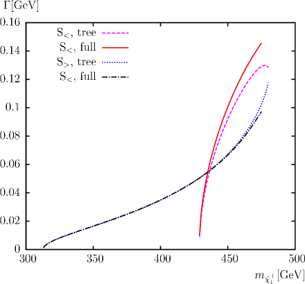
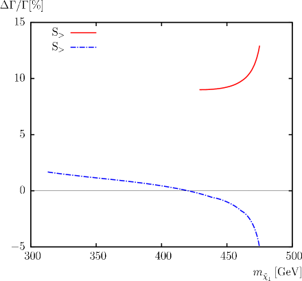
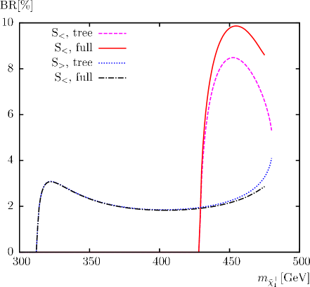
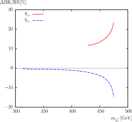
Figure 24: $\Gamma(\tilde{\chi}^{-}_{1}\to\tilde{\chi}^{0}_{1}H^{-})$. Tree-level (“tree”) and full one-loop (“full”) corrected decay widths are shown with the parameters chosen according to ${\cal S}$ (see Tab. 1), with $m_{\tilde{\chi}^{\pm}_{1}}$ varied. The upper left plot shows the decay width, the upper right plot shows the relative size of the corrections. The lower left plot shows the BR, the lower right plot shows the relative size of the BR.

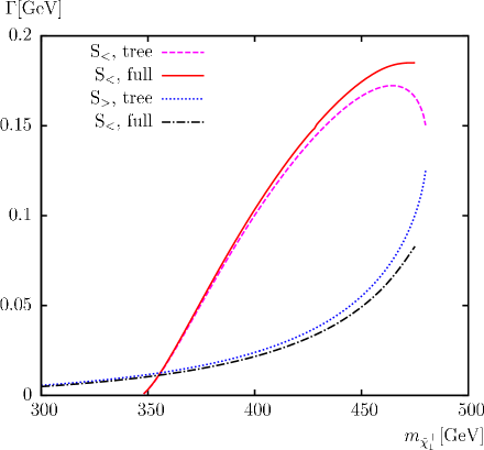
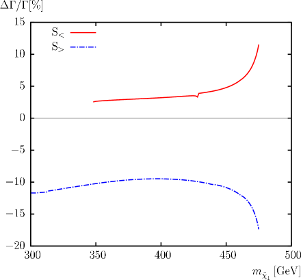
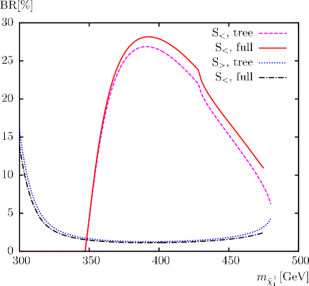
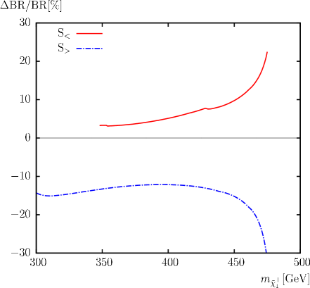
Figure 25: $\Gamma(\tilde{\chi}^{-}_{1}\to\tilde{\chi}^{0}_{1}W^{-})$. Tree-level (“tree”) and full one-loop (“full”) corrected decay widths are shown with the parameters chosen according to ${\cal S}$ (see Tab. 1), with $m_{\tilde{\chi}^{\pm}_{1}}$ varied. The upper left plot shows the decay width, the upper right plot shows the relative size of the corrections. The lower left plot shows the BR, the lower right plot shows the relative size of the BR.

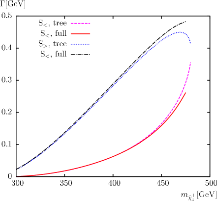
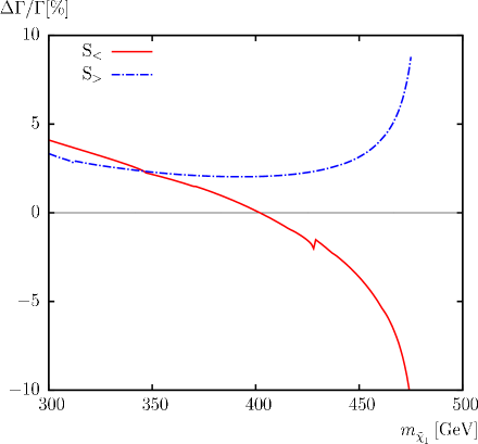
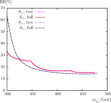
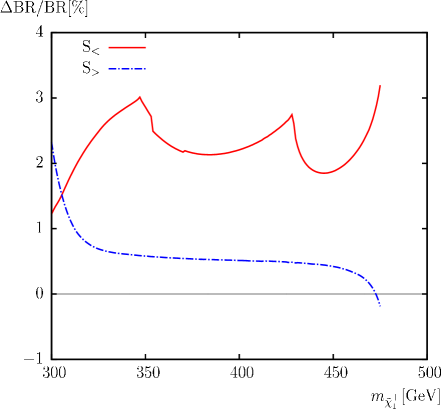
Figure 26: $\Gamma(\tilde{\chi}^{-}_{1}\to\bar{\nu}_{\tau}\,\tilde{\tau}_{1}^{-})$. Tree-level (“tree”) and full one-loop (“full”) corrected decay widths are shown with the parameters chosen according to ${\cal S}$ (see Tab. 1), with $m_{\tilde{\chi}^{\pm}_{1}}$ varied. The upper left plot shows the decay width, the upper right plot shows the relative size of the corrections. The lower left plot shows the BR, the lower right plot shows the relative size of the BR.

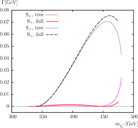
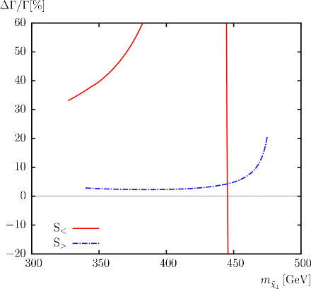
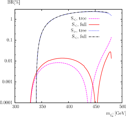
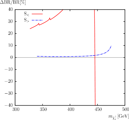
Figure 27: $\Gamma(\tilde{\chi}^{-}_{1}\to\bar{\nu}_{\tau}\,\tilde{\tau}_{2}^{-})$. Tree-level (“tree”) and full one-loop (“full”) corrected decay widths are shown with the parameters chosen according to ${\cal S}$ (see Tab. 1), with $m_{\tilde{\chi}^{\pm}_{1}}$ varied. The upper left plot shows the decay width, the upper right plot shows the relative size of the corrections. The lower left plot shows the BR, the lower right plot shows the relative size of the BR.

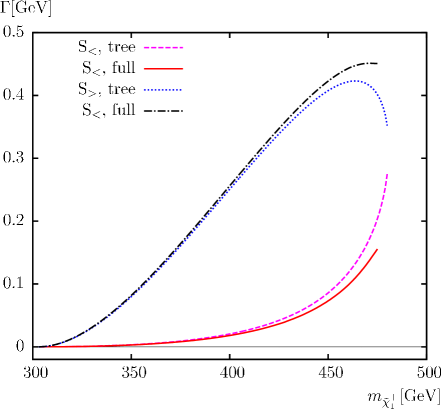
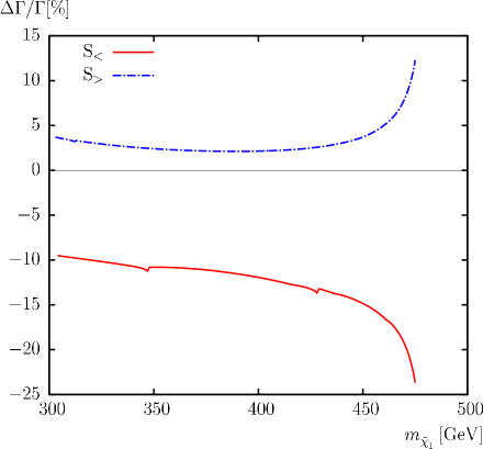
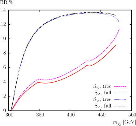
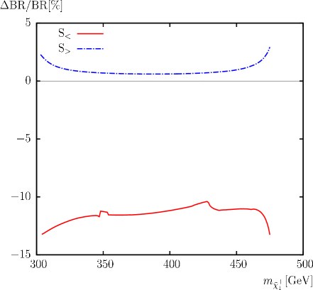
Figure 28: $\Gamma(\tilde{\chi}^{-}_{1}\to\bar{\nu}_{\mu}\,\tilde{\mu}_{1}^{-})$. Tree-level (“tree”) and full one-loop (“full”) corrected decay widths are shown with the parameters chosen according to ${\cal S}$ (see Tab. 1), with $m_{\tilde{\chi}^{\pm}_{1}}$ varied. The upper left plot shows the decay width, the upper right plot shows the relative size of the corrections. The lower left plot shows the BR, the lower right plot shows the relative size of the BR.

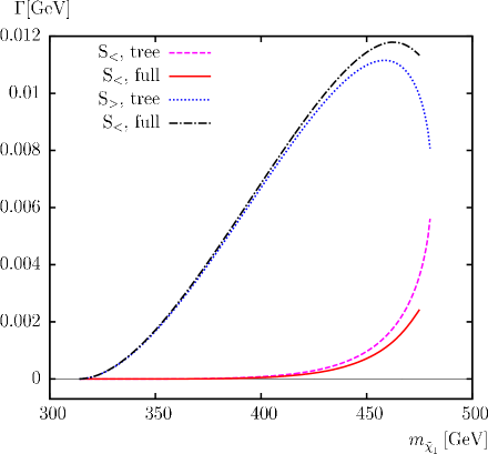
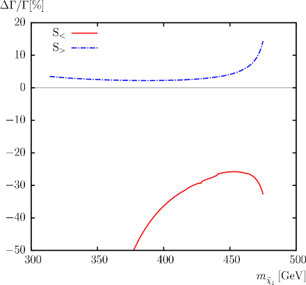
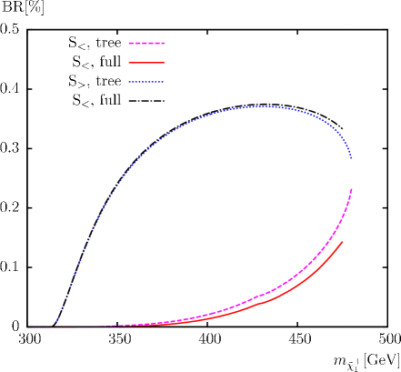
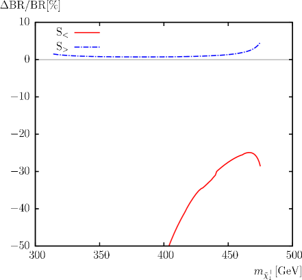
Figure 29: $\Gamma(\tilde{\chi}^{-}_{1}\to\bar{\nu}_{\mu}\,\tilde{\mu}_{2}^{-})$. Tree-level (“tree”) and full one-loop (“full”) corrected decay widths are shown with the parameters chosen according to ${\cal S}$ (see Tab. 1), with $m_{\tilde{\chi}^{\pm}_{1}}$ varied. The upper left plot shows the decay width, the upper right plot shows the relative size of the corrections. The lower left plot shows the BR, the lower right plot shows the relative size of the BR.

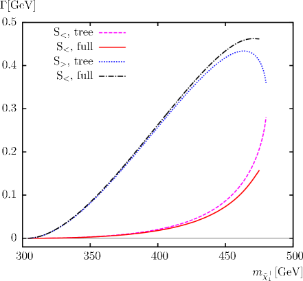
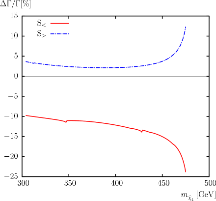
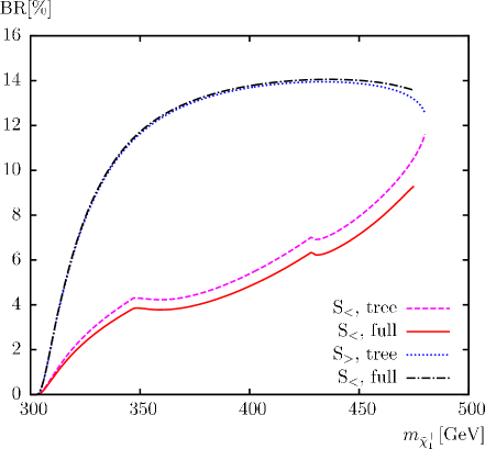
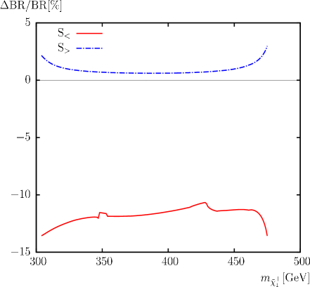
Figure 30: $\Gamma(\tilde{\chi}^{-}_{1}\to\bar{\nu}_{e}\,\tilde{e}_{1}^{-})$. Tree-level (“tree”) and full one-loop (“full”) corrected decay widths are shown with the parameters chosen according to ${\cal S}$ (see Tab. 1), with $m_{\tilde{\chi}^{\pm}_{1}}$ varied. The upper left plot shows the decay width, the upper right plot shows the relative size of the corrections. The lower left plot shows the BR, the lower right plot shows the relative size of the BR.

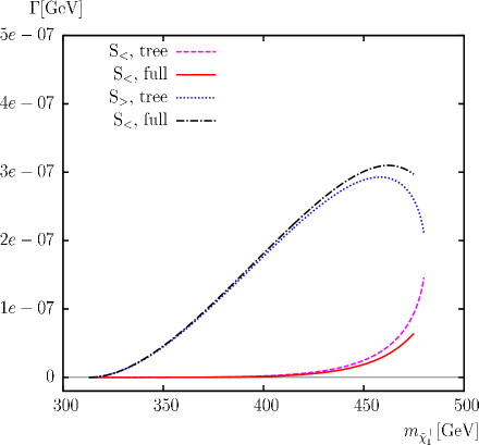
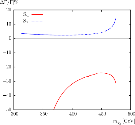
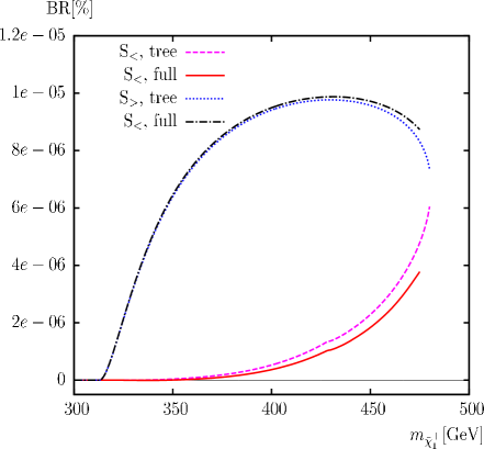
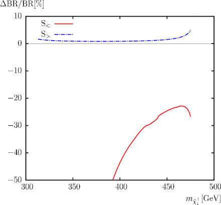
Figure 31: $\Gamma(\tilde{\chi}^{-}_{1}\to\bar{\nu}_{e}\,\tilde{e}_{2}^{-})$. Tree-level (“tree”) and full one-loop (“full”) corrected decay widths are shown with the parameters chosen according to ${\cal S}$ (see Tab. 1), with $m_{\tilde{\chi}^{\pm}_{1}}$ varied. The upper left plot shows the decay width, the upper right plot shows the relative size of the corrections. The lower left plot shows the BR, the lower right plot shows the relative size of the BR.

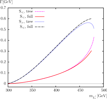
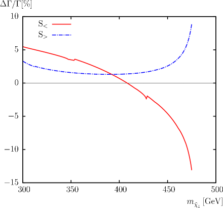
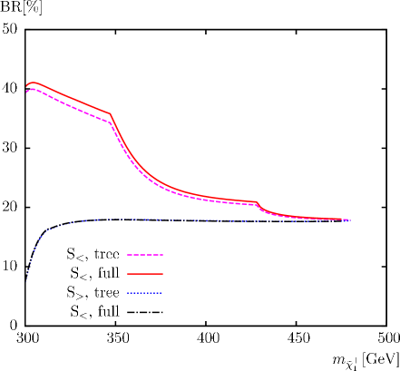
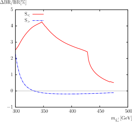
Figure 32: $\Gamma(\tilde{\chi}^{-}_{1}\to{\tau}^{-}\,\tilde{\nu}_{\tau}^{\dagger})$. Tree-level (“tree”) and full one-loop (“full”) corrected decay widths are shown with the parameters chosen according to ${\cal S}$ (see Tab. 1), with $m_{\tilde{\chi}^{\pm}_{1}}$ varied. The upper left plot shows the decay width, the upper right plot shows the relative size of the corrections. The lower left plot shows the BR, the lower right plot shows the relative size of the BR.

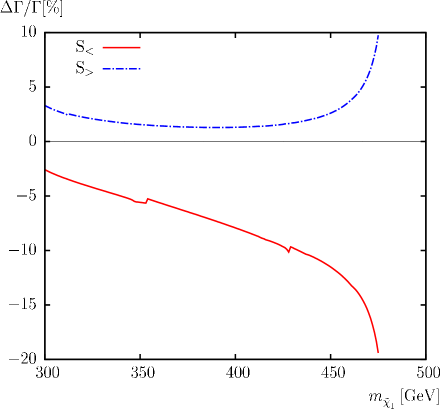
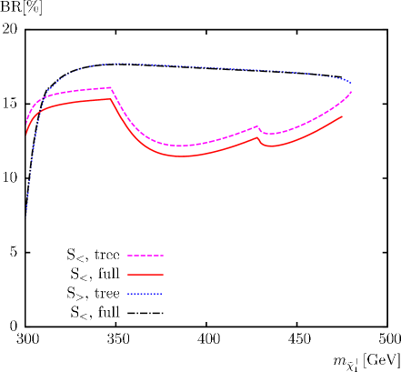
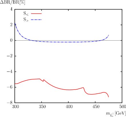
Figure 33: $\Gamma(\tilde{\chi}^{-}_{1}\to{\mu}^{-}\,\tilde{\nu}_{\mu}^{\dagger})$. Tree-level (“tree”) and full one-loop (“full”) corrected decay widths are shown with the parameters chosen according to ${\cal S}$ (see Tab. 1), with $m_{\tilde{\chi}^{\pm}_{1}}$ varied. The upper left plot shows the decay width, the upper right plot shows the relative size of the corrections. The lower left plot shows the BR, the lower right plot shows the relative size of the BR.

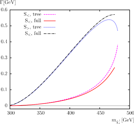
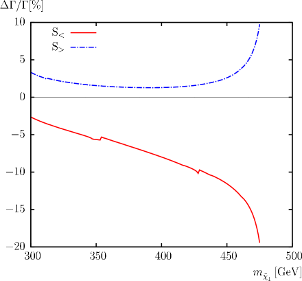
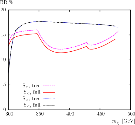
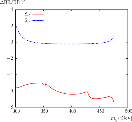
Figure 34: $\Gamma(\tilde{\chi}^{-}_{1}\to{e}^{-}\,\tilde{\nu}_{e}^{\dagger})$. Tree-level (“tree”) and full one-loop (“full”) corrected decay widths are shown with the parameters chosen according to ${\cal S}$ (see Tab. 1), with $m_{\tilde{\chi}^{\pm}_{1}}$ varied. The upper left plot shows the decay width, the upper right plot shows the relative size of the corrections. The lower left plot shows the BR, the lower right plot shows the relative size of the BR.

4.4 Full one-loop results for varying $\varphi_{M_{1}}$

As in the previous sections, the results shown in this subsection consist of “tree”, which denotes the tree-level value and of “full”, which is the decay width including all one-loop corrections as described in Sect. 3. We also show the result leaving out the contributions from absorptive parts of the one-loop self-energy corrections as discussed in Sect. 2, labelled as “full R”. We concentrate on the dependence on $\varphi_{M_{1}}$ for the decays with a final neutralino. For all other decays with no external neutralinos, the neutralinos appear only as virtual particles in the loops, resulting in a negligible dependence on $\varphi_{M_{1}}$. It should be noted, however, that all decay channels must be computed to obtain the correct branching ratios. The parameters are chosen according to Tab. 1, and consequently the full parameter range is accessible at the ILC(1000).

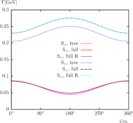
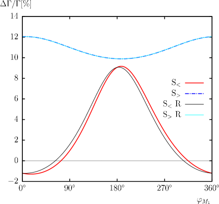
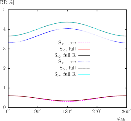
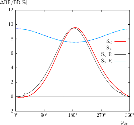
Figure 35: $\Gamma(\tilde{\chi}^{-}_{2}\to\tilde{\chi}^{0}_{1}H^{-})$. Tree-level (“tree”) and full one-loop (“full”) corrected decay widths are shown with the parameters chosen according to ${\cal S}$ (see Tab. 1), with $\phi_{M_{1}}$ varied. Also shown are the full one-loop corrected decay widths omitting the absorptive contributions (“full R”). The upper left plot shows the decay width, the upper right plot shows the relative size of the corrections. The lower left plot shows the BR, the lower right plot shows the relative size of the BR.

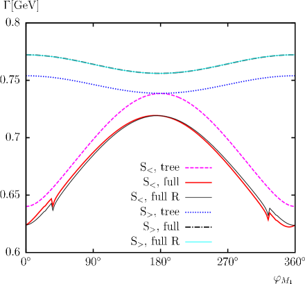
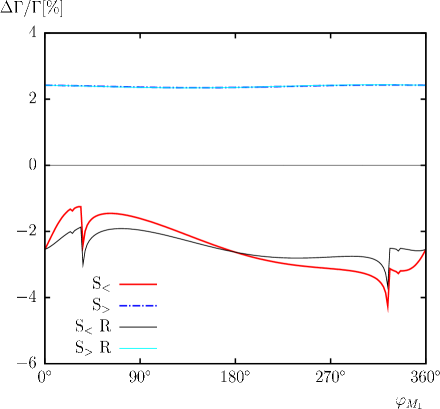
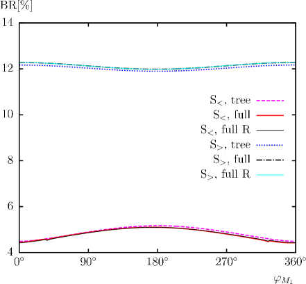
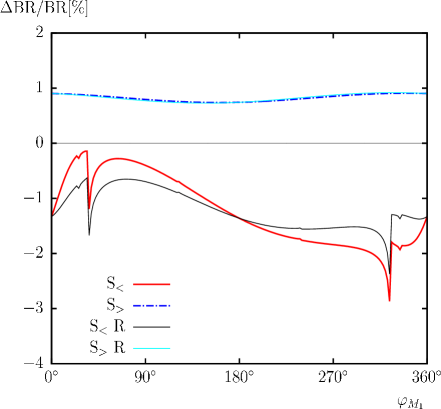
Figure 36: $\Gamma(\tilde{\chi}^{-}_{2}\to\tilde{\chi}^{0}_{2}H^{-})$. Tree-level (“tree”) and full one-loop (“full”) corrected decay widths are shown with the parameters chosen according to ${\cal S}$ (see Tab. 1), with $\phi_{M_{1}}$ varied. Also shown are the full one-loop corrected decay widths omitting the absorptive contributions (“full R”). The upper left plot shows the decay width, the upper right plot shows the relative size of the corrections. The lower left plot shows the BR, the lower right plot shows the relative size of the BR.

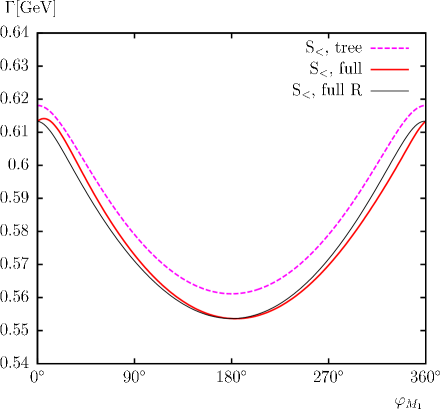
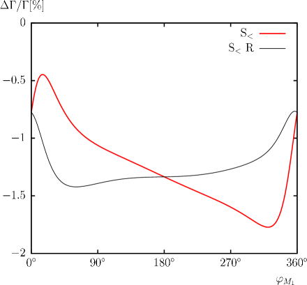
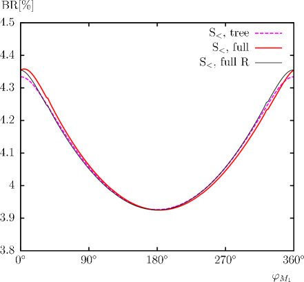
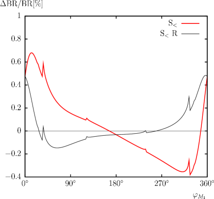
Figure 37: $\Gamma(\tilde{\chi}^{-}_{2}\to\tilde{\chi}^{0}_{3}H^{-})$. Tree-level (“tree”) and full one-loop (“full”) corrected decay widths are shown with the parameters chosen according to ${\cal S}$ (see Tab. 1), with $\phi_{M_{1}}$ varied. Also shown are the full one-loop corrected decay widths omitting the absorptive contributions (“full R”). The upper left plot shows the decay width, the upper right plot shows the relative size of the corrections. The lower left plot shows the BR, the lower right plot shows the relative size of the BR.

In Figs. 35 – 37 we present the results for the decays involving the charged Higgs boson, $\tilde{\chi}^{-}_{2}\to\tilde{\chi}^{0}_{1,2,3}H^{-}$. The decay to the lightest neutralino (see Fig. 35) reaches decay widths around $0.25\ (0.07)\,\,\mathrm{GeV}$ in ${\cal S}_{>}$ (${\cal S}_{<}$), where the dependence on $\varphi_{M_{1}}$ in the latter is substantial, varying between $-1\%$ and $+9\%$. The inclusion of the absorptive self-energy parts, on the other hand, yields only a small effect for the parameter chosen here. The ${\rm BR}(\tilde{\chi}^{-}_{2}\to\tilde{\chi}^{0}_{1}H^{-})$ stays below $1\%$ in ${\cal S}_{<}$ and reaches around $4\%$ in ${\cal S}_{>}$. Here also the one-loop effects on the BR are substantial around $+9\%$. Consequently, an analysis of $\varphi_{M_{1}}$ at the ILC(1000) requires the inclusion of the full one-loop corrections.

The case of $\tilde{\chi}^{-}_{2}\to\tilde{\chi}^{0}_{2}H^{-}$ is shown in Fig. 36. The dips, best visible again in the upper right panel are due to the $\tilde{\chi}^{0}_{2}\to\tilde{\chi}^{0}_{1}Z$ threshold, at $\varphi_{M_{1}}=15^{\circ}$ and the $\tilde{\chi}^{0}_{2}\to\tilde{\chi}^{0}_{1}h_{1}$ threshold, at $\varphi_{M_{1}}=28^{\circ}$. Due to ${\cal CPT}$-invariance the masses are invariant under $\varphi_{M_{1}}\to-\varphi_{M_{1}}$ and mirrored dips are observed at $\varphi_{M_{1}}=332^{\circ}$ and $\varphi_{M_{1}}=345^{\circ}$. Notice that at tree-level the lightest Higgs boson $h_{1}$ and the $Z$ boson are typically almost degenerate. The widths reach values around $\sim 0.7\,\,\mathrm{GeV}$ in both scenarios, leading to branching rations at the level of $12\%$ in ${\cal S}_{>}$ and $4.5\%$ in ${\cal S}_{<}$ with a small variation due to $\varphi_{M_{1}}$. Again the effects of the absorptive self-energy contributions are small. The relative effect of the one-loop corrections is also small at the level of $\pm 1\%$, roughly at the level of the anticipated ILC(1000) precision.

Since the decay $\tilde{\chi}^{-}_{2}\to\tilde{\chi}^{0}_{3}H^{-}$ (Fig. 37) is kinematically forbidden in ${\cal S}_{>}$ we show it only for ${\cal S}_{<}$. We find ${\rm BR}(\tilde{\chi}^{-}_{2}\to\tilde{\chi}^{0}_{3}H^{-})\sim 4\%$, again with a small variation with $\varphi_{M_{1}}$. The effects of the absorptive self-energy contributions is visible at the level of $\sim 1\%$ in the corrections to $\Gamma(\tilde{\chi}^{-}_{2}\to\tilde{\chi}^{0}_{3}H^{-})$, whereas the one-loop effects on the BR is below $\pm 1\%$.

Now we turn to the decays involving a $W$ boson, $\tilde{\chi}^{-}_{2}\to\tilde{\chi}^{0}_{1,2,3}W^{-}$, as shown in Figs. 38 – 40. For $\Gamma(\tilde{\chi}^{-}_{2}\to\tilde{\chi}^{0}_{1}W^{-})$ we find values of $\sim 0.34\,\,\mathrm{GeV}$ in ${\cal S}_{>}$ with a small dependence on $\varphi_{M_{1}}$ and values between $0.03\,\,\mathrm{GeV}$ and $0.18\,\,\mathrm{GeV}$ with a large dependence on $\varphi_{M_{1}}$. The one-loop effects appear at the level of $+5\%$ and $-5\%$, respectively, where in the latter case a sizable effect of the absorptive self-energy contributions can be observed. The ${\rm BR}(\tilde{\chi}^{-}_{2}\to\tilde{\chi}^{0}_{1}W^{-})$ yield $\sim 5\%$ in ${\cal S}_{>}$ and $\sim 1\%$ in ${\cal S}_{<}$, where the one-loop effects are found to be $\sim 4\%$ (${\cal S}_{>}$) and between $-9\%$ and $+2\%$ (${\cal S}_{<}$). Especially in the latter case a reliable ILC analysis requires the inclusion of the full one-loop calculation.

The decay $\tilde{\chi}^{-}_{2}\to\tilde{\chi}^{0}_{2}W^{-}$ (see Fig. 39) yields decay widths around $\sim 1\,\,\mathrm{GeV}$ in both scenarios, corresponding to BR’s of $\sim 16\%$ in ${\cal S}_{>}$ and $\sim 7\%$ in ${\cal S}_{<}$, with a small dependence on $\varphi_{M_{1}}$. The same dips as in $\tilde{\chi}^{-}_{2}\to\tilde{\chi}^{0}_{2}H^{-}$ can be observed. The one-loop effects on the BR’s is found to be $\sim-4\%$ and the variation with $\varphi_{M_{1}}$ is small after the inclusion of the absorptive self-energy contributions, as can be seen in the lower right panel. However, the size of the corrections still exceed the anticipated ILC(1000) accuracy.

The last decay, $\tilde{\chi}^{-}_{2}\to\tilde{\chi}^{0}_{3}W^{-}$ (Fig. 40), which is again only realized in ${\cal S}_{<}$, gives a BR around $\sim 6\%$, where the one-loop corrections can be substantial at the level of $-7\%$. Again, the variation with $\varphi_{M_{1}}$ becomes small after the inclusion of the absorptive self-energy contributions.

Finally we discuss the two relevant $\tilde{\chi}^{-}_{1}$ decays. In Fig. 41 we present the results for $\tilde{\chi}^{-}_{1}\to\tilde{\chi}^{0}_{1}H^{-}$. The decay is kinematically allowed only in ${\cal S}_{>}$ (with the other parameters chosen according to Tab. 1). The decay width is small, not exceeding $0.017\,\,\mathrm{GeV}$, corresponding to a ${\rm BR}(\tilde{\chi}^{-}_{1}\to\tilde{\chi}^{0}_{1}H^{-})$ below $2.5\%$. The variation with $\varphi_{M_{1}}$ is small. The effect of the absorptive self-energy contributions is negligible in both scenarios. In view of the anticipated ILC(1000) accuracy at the per-cent level these corrections should still be taken into account for a reliable analysis.

The last decay is $\tilde{\chi}^{-}_{1}\to\tilde{\chi}^{0}_{1}W^{-}$ shown in Fig. 42. While in ${\cal S}_{>}$ the decay is kinematically allowed for the full range of $\varphi_{M_{1}}$ only in ${\cal S}_{>}$, while in ${\cal S}_{<}$ it remains kinematically forbidden for $120^{\circ}\leq\varphi_{M_{1}}\leq 240^{\circ}$. The decay widths are below $0.012\ (0.004)\,\,\mathrm{GeV}$ in ${\cal S}_{>}$ (${\cal S}_{<}$), corresponding to BR’s at the level of $\sim 1\%$ (${\cal S}_{>}$) and between $\sim 4\%$ and $0\%$ (${\cal S}_{<}$). Here a strong dependence on $\varphi_{M_{1}}$ is visible. The size of the one-loop effects exceed $-15\%$ in ${\cal S}_{>}$ and are around $+4\%$ in ${\cal S}_{<}$. The effect of the absorptive self-energy contributions is negligible. As before, the corrections are potentially relevant for an ILC(1000) analysis.

We have also analyzed the effects of a variation with $\varphi_{A_{\tau}}$, but found negligible effects for the parameters in Tab. 1. The situation would be different if the off-diagonal element in the scalar tau mass matrix, $X_{\tau}=A_{\tau}-\mu\tan\beta$ were depending strongly on $A_{\tau}$, i.e. for small $\mu$ and/or $\tan\beta$. However, a detailed analysis of these effects is beyond the scope of our paper.

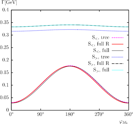
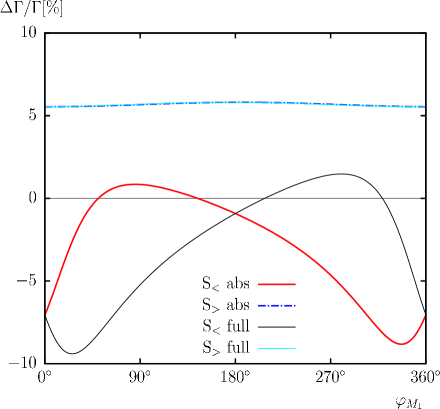
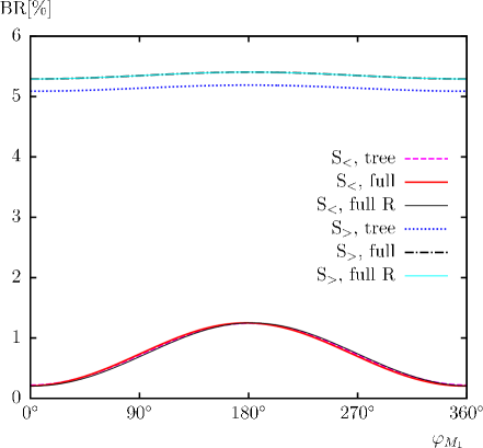
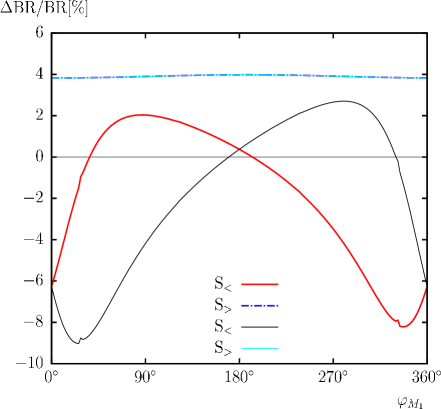
Figure 38: $\Gamma(\tilde{\chi}^{-}_{2}\to\tilde{\chi}^{0}_{1}W^{-})$. Tree-level (“tree”) and full one-loop (“full”) corrected decay widths are shown with the parameters chosen according to ${\cal S}$ (see Tab. 1), with $\phi_{M_{1}}$ varied. Also shown are the full one-loop corrected decay widths omitting the absorptive contributions (“full R”). The upper left plot shows the decay width, the upper right plot shows the relative size of the corrections. The lower left plot shows the BR, the lower right plot shows the relative size of the BR.

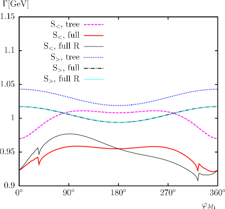
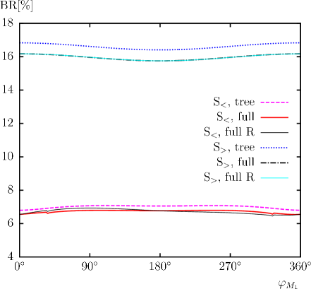
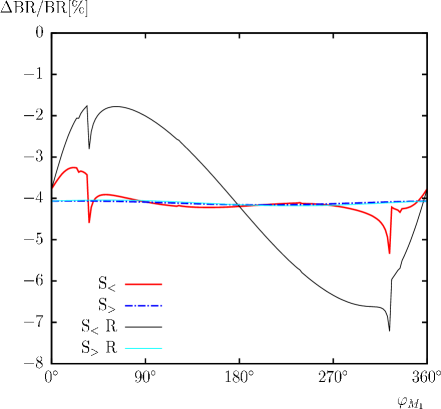
Figure 39: $\Gamma(\tilde{\chi}^{-}_{2}\to\tilde{\chi}^{0}_{2}W^{-})$. Tree-level (“tree”) and full one-loop (“full”) corrected decay widths are shown with the parameters chosen according to ${\cal S}$ (see Tab. 1), with $\phi_{M_{1}}$ varied. Also shown are the full one-loop corrected decay widths omitting the absorptive contributions (“full R”). The upper left plot shows the decay width, the upper right plot shows the relative size of the corrections. The lower left plot shows the BR, the lower right plot shows the relative size of the BR.

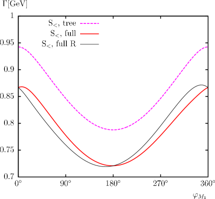
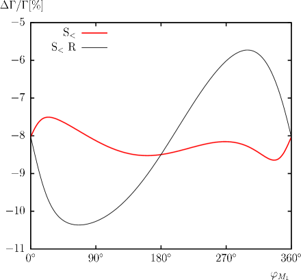
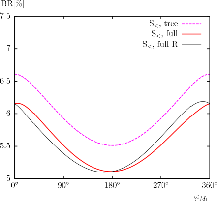
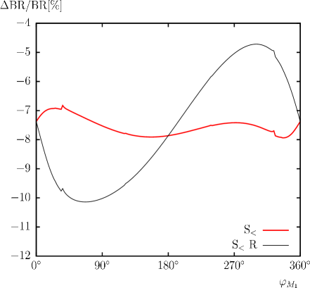
Figure 40: $\Gamma(\tilde{\chi}^{-}_{2}\to\tilde{\chi}^{0}_{3}W^{-})$. Tree-level (“tree”) and full one-loop (“full”) corrected decay widths are shown with the parameters chosen according to ${\cal S}$ (see Tab. 1), with $\phi_{M_{1}}$ varied. Also shown are the full one-loop corrected decay widths omitting the absorptive contributions (“full R”). The upper left plot shows the decay width, the upper right plot shows the relative size of the corrections. The lower left plot shows the BR, the lower right plot shows the relative size of the BR.

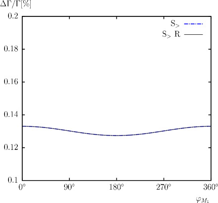
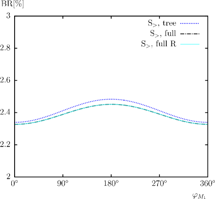
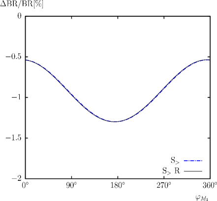
Figure 41: $\Gamma(\tilde{\chi}^{-}_{1}\to\tilde{\chi}^{0}_{1}H^{-})$. Tree-level (“tree”) and full one-loop (“full”) corrected decay widths are shown with the parameters chosen according to ${\cal S}$ (see Tab. 1), with $\phi_{M_{1}}$ varied. Also shown are the full one-loop corrected decay widths omitting the absorptive contributions (“full R”). The upper left plot shows the decay width, the upper right plot shows the relative size of the corrections. The lower left plot shows the BR, the lower right plot shows the relative size of the BR.

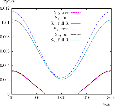
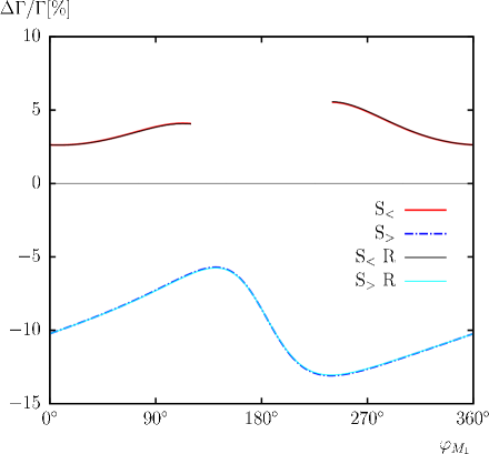
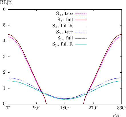
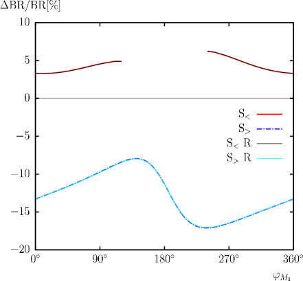
Figure 42: $\Gamma(\tilde{\chi}^{-}_{1}\to\tilde{\chi}^{0}_{1}W^{-})$. Tree-level (“tree”) and full one-loop (“full”) corrected decay widths are shown with the parameters chosen according to ${\cal S}$ (see Tab. 1), with $\phi_{M_{1}}$ varied. Also shown are the full one-loop corrected decay widths omitting the absorptive contributions (“full R”). The upper left plot shows the decay width, the upper right plot shows the relative size of the corrections. The lower left plot shows the BR, the lower right plot shows the relative size of the BR.

4.5 Full one-loop results: total decay widths

In this final subsection we briefly show the results for the total decay widths in Fig. 43. The results for $\tilde{\chi}^{\pm}_{2}$ are shown in the upper row. The total width rises from its lowest values at $m_{\tilde{\chi}^{\pm}_{2}}=475\,\,\mathrm{GeV}$ to about $13\,\,\mathrm{GeV}$ at $m_{\tilde{\chi}^{\pm}_{2}}=1000\,\,\mathrm{GeV}$ in ${\cal S}_{>}$. In ${\cal S}_{<}$ the width goes up to $34\,\,\mathrm{GeV}$, once loop corrections are included. The overall size of the one-loop corrections varies strongly with $m_{\tilde{\chi}^{\pm}_{2}}$ as can be seen in the upper right plot. Values of $\pm 5\%$ can easily be reached.

In the lower row of Fig. 43 we show the total width of the lighter chargino. It rises only up to about $3.3\,\,\mathrm{GeV}$ in ${\cal S}_{>}$ and $\sim 1.5\,\,\mathrm{GeV}$ in ${\cal S}_{<}$. Again the size of the one-loop corrections vary with $m_{\tilde{\chi}^{\pm}_{1}}$, where away from threshold we find corrections at the level of $+2\%$ in ${\cal S}_{>}$ and between $+2\%$ and $\sim-10\%$ in ${\cal S}_{<}$.

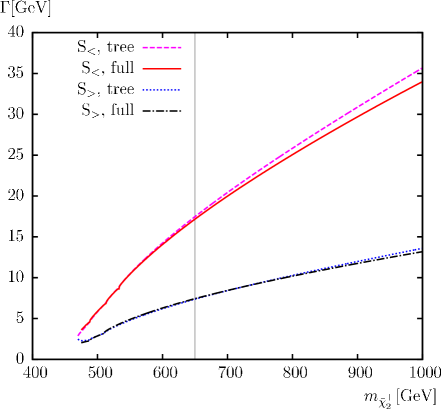
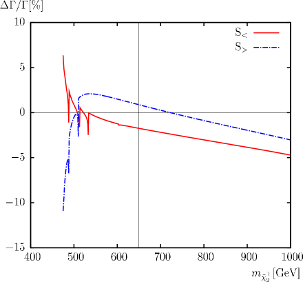
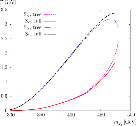
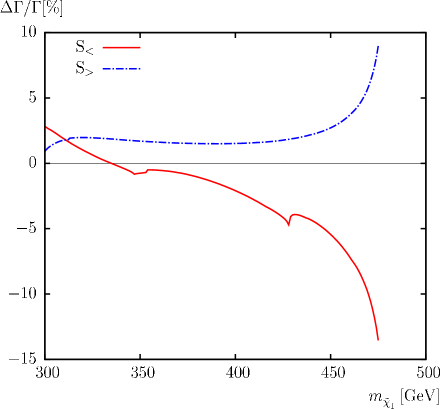
Figure 43: $\Gamma(\tilde{\chi}^{-}_{i}\to all)$, $i=1,2$. Tree-level (“tree”) and full one-loop (“full”) corrected total decay widths are shown with the parameters chosen according to ${\cal S}$ (see Tab. 1), with $m_{\tilde{\chi}^{\pm}_{i}}$ varied. The upper left plot shows the decay width of $\tilde{\chi}^{-}_{2}$ and the upper right plot shows the corresponding relative size of the corrections, both as a function of its mass. The lower left and right plots show the same observables for $\tilde{\chi}^{-}_{1}$. The vertical lines indicate where $m_{\tilde{\chi}^{\pm}_{1}}+m_{\tilde{\chi}^{\pm}_{2}}=1000\,\,\mathrm{GeV}$, i.e. the maximum reach of the ILC(1000) for $\tilde{\chi}^{\pm}_{1}\tilde{\chi}^{\mp}_{2}$ pair production.

5 Conclusions

We have evaluated two-body decay widths of charginos in the Minimal Supersymmetric Standard Model with complex parameters (cMSSM). Assuming heavy scalar quarks we take into account all decay channels involving charginos, neutralinos, (scalar) leptons, Higgs bosons and SM gauge bosons. The decay modes are given in Eqs. (1) – (6). The evaluation of the decay widths is based on a full one-loop calculation including hard and soft QED radiation. Such a calculation is necessary to derive a reliable prediction of any two-body branching ratio. Three-body decay modes can become sizable only if all the two-body channels are kinematically (nearly) closed and have thus been neglected throughout the paper. The same applies to two-body decay modes that appear only at the one-loop level.

We first reviewed the one-loop renormalization of the cMSSM, which is relevant for our calculation. We have given details for the lepton/slepton sector, whereas the details for the chargino/neutralino and the Higgs boson sector can be found in Ref. [28].

We have discussed the calculation of the one-loop diagrams, the treatment of UV- and IR-divergences that are canceled by the inclusion of soft QED radiation. Our calculation set-up can easily be extended to other two-body decays involving (scalar) quarks.

For the numerical analysis we have chosen a parameter set that allows simultaneously all two-body decay modes under investigation (but could potentially be in conflict with the most recent SUSY search results from the LHC). The masses of the charginos in this scenario are $600$ and $350\,\,\mathrm{GeV}$. This scenario allows copious production of the charginos in SUSY cascades at the LHC. Furthermore, the production of $\tilde{\chi}^{\pm}_{1}\tilde{\chi}^{\mp}_{2}$ or $\tilde{\chi}^{+}_{1}\tilde{\chi}^{-}_{1}$ at the ILC(1000), i.e. with $\sqrt{s}=1000\,\,\mathrm{GeV}$, via $e^{+}e^{-}\to\tilde{\chi}^{\pm}_{1,2}\tilde{\chi}^{\mp}_{1}$ will be possible, with all the subsequent decay modes (1) – (6) being (in principle) open. The clean environment of the ILC would then permit a detailed, statistically dominated study of the chargino decays. Depending on the channel and the polarization, a precision at the per-cent level seems to be achievable. Special attention is paid to chargino decays involving the Lightest Supersymmetric Particle (LSP), i.e. the lightest neutralino, or a neutral or charged Higgs boson.

In our numerical analysis we have shown results for varying $m_{\tilde{\chi}^{\pm}_{1,2}}$ and $\varphi_{M_{1}}$, the phase of the soft SUSY-breaking parameter $M_{1}$. In the results with varied chargino masses only the lighter values allow $\tilde{\chi}^{\pm}_{1}\tilde{\chi}^{\mp}_{2}$ production at the ILC(1000), whereas the results with varied $\varphi_{M_{1}}$ have sufficiently light charginos to permit $e^{+}e^{-}\to\tilde{\chi}^{\pm}_{1}\tilde{\chi}^{\mp}_{2}$. In the numerical analysis we compared the tree-level width with the one-loop corrected decay width. In the analysis with $\varphi_{M_{1}}$ varied we explicitly took into account contributions from the absorptive parts of self-energy contributions on external legs. We also analyzed the relative change of the width to demonstrate the size of the loop corrections on each individual channel. In order to see the effect on the experimentally accessible quantities we also show the various branching ratios at tree-level (all channels are evaluated at tree-level) and at the one-loop level (with all channels evaluated including the full one-loop contributions). Furthermore we presented the relative change of the BRs that can directly be compared with the anticipated experimental accuracy.

We found sizable corrections in many of the decay channels. Especially, the higher-order corrections of the chargino decay widths involving the LSP can easily reach a level of about $\pm 10\%$. Decay modes involving Higgs bosons turn out to have slightly smaller corrections. The size of the full one-loop corrections to the decay widths and the branching ratios also depends strongly on $\varphi_{M_{1}}$. The one-loop contributions, again being roughly of ${\cal O}(5\%)$, often vary by a factor of $2-3$ as a function of $\varphi_{M_{1}}$. All results on partial decay widths are given in detail in Sects. 4.2 – 4.4, while the total decay widths are shown in Sect. 4.5.

The numerical results we have shown are of course dependent on choice of the SUSY parameters. Nevertheless, they give an idea of the relevance of the full one-loop corrections. For other choices of SUSY masses the corrections to the decay widths would stay the same, but the branching ratios would look very different. Channels (and their respective one-loop corrections) that may look unobservable due to the smallness of their BR in our numerical examples could become important if other channels are kinematically forbidden.

Following our analysis it is evident that the full one-loop corrections are mandatory for a precise prediction of the various branching ratios. This applies to LHC analyses, but even more to analyses at the ILC, where a precision at the per-cent level is anticipated for the determination of chargino branching ratios (depending on the chargino masses, the center-of-mass energy and the integrated luminosity). The results for the chargino decays will be implemented into the Fortran code FeynHiggs.

Acknowledgements

We thank A. Bharucha, M. Drees, A. Fowler, H. Haber, T. Hahn, O. Kittel, S. Liebler, H. Rzehak and G. Weiglein for helpful discussions. The work of S.H. was partially supported by CICYT (grant FPA 2007–66387 and FPA 2010–22163-C02-01). F.v.d.P. was supported by the Spanish MICINN’s Consolider-Ingenio 2010 Programme under grant MultiDark CSD2009-00064.

References

-
[1]
H.P. Nilles,
Phys. Rep. 110 (1984) 1;
H.E. Haber and G.L. Kane, Phys. Rep. 117 (1985) 75;
R. Barbieri, Riv. Nuovo Cim. 11 (1988) 1. -
[2]
H. Goldberg,
Phys. Rev. Lett. 50 (1983) 1419;
J. Ellis, J. Hagelin, D. Nanopoulos, K. Olive and M. Srednicki, Nucl. Phys. B 238 (1984) 453. -
[3]
A. Pilaftsis,
Phys. Rev. D 58 (1998) 096010
[arXiv:hep-ph/9803297];
A. Pilaftsis, Phys. Lett. B 435 (1998) 88 [arXiv:hep-ph/9805373]. - [4] A. Pilaftsis and C. Wagner, Nucl. Phys. B 553 (1999) 3 [arXiv:hep-ph/9902371].
- [5] S. Heinemeyer, Eur. Phys. J. C 22 (2001) 521 [arXiv:hep-ph/0108059].
- [6] G. Aad et al. [The ATLAS Collaboration], arXiv:0901.0512.
- [7] G. Bayatian et al. [CMS Collaboration], J. Phys. G 34 (2007) 995.
-
[8]
TESLA Technical Design Report [TESLA Collaboration] Part 3,
“Physics at an Linear Collider”,
arXiv:hep-ph/0106315,
see:
tesla.desy.de/new_pages/TDR_CD/start.html;
K. Ackermann et al., DESY-PROC-2004-01. -
[9]
J. Brau et al. [ILC Collaboration],
ILC Reference Design Report Volume 1 - Executive Summary,
arXiv:0712.1950 [physics.acc-ph];
G. Aarons et al. [ILC Collaboration], International Linear Collider Reference Design Report Volume 2: Physics at the ILC, arXiv:0709.1893 [hep-ph];
E. Accomando et al. [ CLIC Physics Working Group Collaboration ], arXiv:hep-ph/0412251. -
[10]
G. Weiglein et al. [LHC/ILC Study Group],
Phys. Rept. 426 (2006) 47
[arXiv:hep-ph/0410364];
A. De Roeck et al., Eur. Phys. J. C 66 (2010) 525 [arXiv:0909.3240 [hep-ph]];
A. De Roeck, J. Ellis, S. Heinemeyer, CERN Cour. 49N10 (2009) 27. - [11] S. AbdusSalam, et al., arXiv:1109.3859 [hep-ph].
-
[12]
J. F. Gunion, H. E. Haber, R. M. Barnett, M. Drees, D. Karatas, X. Tata and H. Baer,
Int. J. Mod. Phys. A 2 (1987) 1145;
H. Baer, A. Bartl, D. Karatas, W. Majerotto and X. Tata, Int. J. Mod. Phys. A 4 (1989) 4111. - [13] J. Gunion and H. Haber, Phys. Rev. D 37 (1988) 2515.
- [14] J. Gunion and H. Haber, Nucl. Phys. B 307 (1988) 445.
-
[15]
R. Zhang, W. Ma, L. Wan,
J. Phys. G 28 (2002) 169
[arXiv:hep-ph/0111124];
P.-J. Zhou, W.-G. Ma, R.-Y. Zhang and L.-H. Wan, Commun. Theor. Phys. 38 (2002) 173. - [16] A. Djouadi, Y. Mambrini and M. Mühlleitner, Eur. Phys. J. C 20 (2001) 563 [arXiv:hep-ph/0104115].
- [17] K. Rolbiecki, arXiv:0710.1748 [hep-ph].
- [18] N. Baro and F. Boudjema, Phys. Rev. D 80 (2009) 076010 [arXiv:0906.1665 [hep-ph]].
- [19] J. Fujimoto, T. Ishikawa, Y. Kurihara, M. Jimbo, T. Kon and M. Kuroda, Phys. Rev. D 75 (2007) 113002.
- [20] M. Mühlleitner, A. Djouadi and Y. Mambrini, Comput. Phys. Commun. 168 (2005) 46 [arXiv:hep-ph/0311167].
- [21] S. Liebler and W. Porod, Nucl. Phys. B 849 (2011) 213 [Erratum-ibid. B 856 (2012) 125] [arXiv:1011.6163 [hep-ph]].
- [22] W. Yang and D. Du, Phys. Rev. D 67 (2003) 055004 [arXiv:hep-ph/0211453].
- [23] H. Eberl, T. Gajdosik, W. Majerotto and B. Schrausser, Phys. Lett. B 618 (2005) 171 [arXiv:hep-ph/0502112].
- [24] S. Heinemeyer, W. Hollik and G. Weiglein, Comput. Phys. Commun. 124 (2000) 76 [arXiv:hep-ph/9812320]; see www.feynhiggs.de .
- [25] S. Heinemeyer, W. Hollik and G. Weiglein, Eur. Phys. J. C 9 (1999) 343 [arXiv:hep-ph/9812472].
- [26] G. Degrassi, S. Heinemeyer, W. Hollik, P. Slavich and G. Weiglein, Eur. Phys. J. C 28 (2003) 133 [arXiv:hep-ph/0212020].
- [27] M. Frank, T. Hahn, S. Heinemeyer, W. Hollik, R. Rzehak and G. Weiglein, JHEP 02 (2007) 047 [arXiv:hep-ph/0611326].
- [28] T. Fritzsche, S. Heinemeyer, H. Rzehak and C. Schappacher, arXiv:1111.7289 [hep-ph].
- [29] S. Heinemeyer, W. Hollik, H. Rzehak and G. Weiglein, Phys. Lett. B 652 (2007) 300 [arXiv:0705.0746 [hep-ph]].
- [30] S. Heinemeyer, H. Rzehak and C. Schappacher, Phys. Rev. D 82 (2010) 075010 [arXiv:1007.0689 [hep-ph]]; PoSCHARGED 2010 (2010) 039 [arXiv:1012.4572 [hep-ph]].
- [31] A. Bartl, H. Eberl, K. Hidaka, S. Kraml, W. Majerotto, W. Porod and Y. Yamada, Phys. Rev. D 59 (1999) 115007 [arXiv:hep-ph/9806299].
- [32] A. Djouadi, P. Gambino, S. Heinemeyer, W. Hollik, C. Jünger and G. Weiglein, Phys. Rev. Lett. 78 (1997) 3626 [arXiv:hep-ph/9612363]; Phys. Rev. D 57 (1998) 4179 [arXiv:hep-ph/9710438].
- [33] W. Hollik and H. Rzehak, Eur. Phys. J. C 32 (2003) 127 [arXiv:hep-ph/0305328].
- [34] S. Heinemeyer, W. Hollik, H. Rzehak and G. Weiglein, Eur. Phys. J. C 39 (2005) 465 [arXiv:hep-ph/0411114].
- [35] R. Peccei and H. Quinn, Phys. Rev. Lett. 38 (1977) 1440; Phys. Rev. D 16 (1977) 1791.
- [36] S. Dimopoulos and S. Thomas, Nucl. Phys. B 465 (1996) 23 [arXiv:hep-ph/9510220].
- [37] D. Demir, Phys.Rev. D 60 (1999) 055006 [arXiv:hep-ph/9901389].
- [38] M. Carena, J. Ellis, A. Pilaftsis and C. Wagner, Nucl. Phys. B 625 (2002) 345 [arXiv:hep-ph/0111245].
- [39] A. Fowler, PhD thesis: “Higher order and CP-violating effects in the neutralino and Higgs boson sectors of the MSSM”, sector”, Durham University, UK, September 2010.
- [40] T. Fritzsche, PhD thesis, Cuvillier Verlag, Göttingen 2005, ISBN 3–86537–577–4.
-
[41]
T. Fritzsche and W. Hollik,
Eur. Phys. J. C 24 (2002) 619
[arXiv:hep-ph/0203159];
T. Fritzsche, Diploma thesis, Institut für Theoretische Physik, Universität Karlsruhe, Germany, Dec. 2000, see:
www-itp.particle.uni-karlsruhe.de/diplomatheses.de.shtml . - [42] A. Chatterjee, M. Drees, S. Kulkarni, Q. Xu, arXiv:1107.5218 [hep-ph].
-
[43]
J. Küblbeck, M. Böhm and A. Denner,
Comput. Phys. Commun. 60 (1990) 165;
T. Hahn, Comput. Phys. Commun. 140 (2001) 418 [arXiv:hep-ph/0012260];
T. Hahn and C. Schappacher, Comput. Phys. Commun. 143 (2002) 54 [arXiv:hep-ph/0105349].
The program, the user’s guide and the MSSM model files are available via
www.feynarts.de . - [44] T. Hahn and M. Pérez-Victoria, Comput. Phys. Commun. 118 (1999) 153 [arXiv:hep-ph/9807565].
- [45] F. del Aguila, A. Culatti, R. Munoz Tapia and M. Perez-Victoria, Nucl. Phys. B 537 (1999) 561 [arXiv:hep-ph/9806451].
-
[46]
W. Siegel,
Phys. Lett. B 84 (1979) 193;
D. Capper, D. Jones, and P. van Nieuwenhuizen, Nucl. Phys. B 167 (1980) 479. - [47] D. Stöckinger, JHEP 0503 (2005) 076 [arXiv:hep-ph/0503129].
- [48] W. Hollik and D. Stöckinger, Phys. Lett. B 634 (2006) 63 [arXiv:hep-ph/0509298].
- [49] A. Denner, Fortsch. Phys. 41 (1993) 307 [arXiv:0709.1075 [hep-ph]].
- [50] The couplings can be found in the files MSSM.ps.gz, MSSMQCD.ps.gz and HMix.ps.gz as part of the FeynArts package [43].
- [51] K. Nakamura et al. [Particle Data Group], J. Phys. G 37 (2010) 075021.
- [52] M. Dugan, B. Grinstein and L. Hall, Nucl. Phys. B 255 (1985) 413.
- [53] W. Hollik, J. Illana, S. Rigolin and D. Stöckinger, Phys. Lett. B 416 (1998) 345 [arXiv:hep-ph/9707437]; Phys. Lett. B 425 (1998) 322 [arXiv:hep-ph/9711322].
- [54] D. Demir, O. Lebedev, K. Olive, M. Pospelov and A. Ritz, Nucl. Phys. B 680 (2004) 339 [arXiv:hep-ph/0311314].
-
[55]
D. Chang, W. Keung and A. Pilaftsis,
Phys. Rev. Lett. 82 (1999) 900
[Erratum-ibid. 83 (1999) 3972]
[arXiv:hep-ph/9811202];
A. Pilaftsis, Phys. Lett. B 471 (1999) 174 [arXiv:hep-ph/9909485]. - [56] O. Lebedev, K. Olive, M. Pospelov and A. Ritz, Phys. Rev. D 70 (2004) 016003 [arXiv:hep-ph/0402023].
- [57] Y. Li, S. Profumo and M. Ramsey-Musolf, JHEP 1008 (2010) 062 [arXiv:1006.1440 [hep-ph]].
- [58] V. Barger, T. Falk, T. Han, J. Jiang, T. Li and T. Plehn, Phys. Rev. D 64 (2001) 056007 [arXiv:hep-ph/0101106].
-
[59]
The Muon g-2 Collaboration,
Phys. Rev. Lett. 92 (2004) 161802
[arXiv:hep-ex/0401008];
G. Bennett et al. [The Muon g-2 Collaboration], Phys. Rev. D 73 (2006) 072003 [arXiv:hep-ex/0602035]. -
[60]
D. Stöckinger,
J. Phys. G 34 (2007) R45
[arXiv:hep-ph/0609168];
J. Miller, E. de Rafael and B. Roberts, Rept. Prog. Phys. 70 (2007) 795 [arXiv:hep-ph/0703049];
F. Jegerlehner and A. Nyffeler, Phys. Rept. 477 (2009) 1 [arXiv:0902.3360 [hep-ph]];
J. Prades, Acta Phys. Polon. Supp. 3 (2010) 75 [arXiv:0909.2546 [hep-ph]];
T. Teubner, K. Hagiwara, R. Liao, A. Martin and D. Nomura, arXiv:1001.5401 [hep-ph];
K. Hagiwara, R. Liao, A. D. Martin, D. Nomura, T. Teubner, J. Phys. G G38 (2011) 085003 [arXiv:1105.3149 [hep-ph]]. - [61] M. Davier, A. Hoecker, B. Malaescu and Z. Zhang, Eur. Phys. J. C 71 (2011) 1515 [arXiv:1010.4180 [hep-ph]].
- [62] [LEP Higgs working group], Phys. Lett. B 565 (2003) 61 [arXiv:hep-ex/0306033].
- [63] [LEP Higgs working group], Eur. Phys. J. C 47 (2006) 547 [arXiv:hep-ex/0602042].
- [64] H. Dreiner, S. Heinemeyer, O. Kittel, U. Langenfeld, A. Weber and G. Weiglein, Eur. Phys. J. C 62 (2009) 547 [arXiv:0901.3485 [hep-ph]].
-
[65]
T. Blank and W. Hollik,
Nucl. Phys. B 514 (1998) 113
[arXiv:hep-ph/9703392];
W. Öller, H. Eberl and W. Majerotto, Phys. Rev. D 71 (2005) 115002 [arXiv:hep-ph/0504109];
M. Diaz, M. Rivera and D. Ross, JHEP 1004 (2010) 098 [arXiv:0911.4403 [hep-ph]].