Quantum Strategies Win in a Defector-Dominated Population

Abstract

Quantum strategies are introduced into evolutionary games. The agents using quantum strategies are regarded as invaders whose fraction generally is 1% of a population in contrast to the 50% defectors. In this paper, the evolution of strategies on networks is investigated in a defector-dominated population, when three networks (Regular Lattice, Newman-Watts small world network, scale-free network) are constructed and three games (Prisoners’ Dilemma, Snowdrift, Stag-Hunt) are employed. As far as these three games are concerned, the results show that quantum strategies can always invade the population successfully. Comparing the three networks, we find that the regular lattice is most easily invaded by agents that adopt quantum strategies. However, for a scale-free network it can be invaded by agents adopting quantum strategies only if a hub is occupied by an agent with a quantum strategy or if the fraction of agents with quantum strategies in the population is significant.

1 Introduction

Game theory has been widely applied in both social and biological fields, in order to describe interactions between agents. Recently, the evolution of behavior of agents in a population, in the framework of evolutionary games on graphs, has attracted much interdisciplinary attention. Nowak and May [1, 2] firstly introduced the spatial Prisoner’s Dilemma (PD) game, in which agents (players) occupy all vertices of a two-dimensional lattice and the edges represent neighbor relations between the corresponding agents. This pioneering work triggered an intensive investigation of spatial games and the PD game is a model frequently adopted by researchers [3, 4]. It is known that the structure of the network is also a key factor in the evolution of behavior of agents. Later, a shift from evolutionary games on regular lattices to evolutionary games on complex networks was proposed [5], in particular on small world networks [6, 7, 8] and on scale-free networks [9, 10, 11]. Meanwhile, other games, such as Snowdrift (SD) [12], Stag-Hunt (SH) [13], and Public Goods games, have produced interesting results [14, 15, 16, 17].

Surprisingly, the concept of evolutionary games has been extended to the microworld to describe interactions of biological molecules [18, 19, 20, 21], a domain where quantum mechanics defines the laws. Meanwhile, game theory is also generalized to the quantum regime, and a new area called quantum game theory has emerged from the field of quantum computation. In recent years, much interest has been focused on quantum game theory. For instance, Meyer’s results [22] showed that if an agent in a penny flip game is allowed to implement quantum strategies, she/he can always defeat her/his opponent playing a classical strategy and can thus increase her/his expected payoff. Eisert et al. [23] quantized the PD and demonstrated that it is possible to escape the dilemma when both players resort to quantum strategies. Marinatto et al. [24] found a unique equilibrium for the Battle of the Sexes game, when entangled strategies were allowed. Later, evolutionarily stable strategies in quantum games and an evolutionary quantum game were also studied by Iqbal et al. [25] and Kay et al. [26] respectively. Moreover, quantum games have also been implemented using quantum computers [27, 28, 29]. For further background on quantum games, see [30, 31].

In quantum game theory, agents are allowed to use quantum strategies from a quantum strategy set that is a much larger set than a classical one, i.e., a classical strategy set is only a subset of a quantum strategy set. This larger space offers a possibility for a diversity of agent behavior and allows new patterns to emerge. In this paper, we assume all agents in a population are quantum agents who can use quantum strategies to play games with their neighbors and make decisions. However, initially, only a few randomly selected agents, about 1% in the population, are assigned quantum strategies, while the others are players with strategies taken from the classical strategy set. The fraction of defectors is about half of the population. This work discusses how quantum strategies spread in the population and how strategies evolve over repeated games played on networks. Therefore, three networks (Regular Lattice, Newman-Watts small world network, scale-free network) are constructed and three games (Prisoners’ Dilemma, Snowdrift, Stag-Hunt) are employed. The games encapsulate agents’ responses to different external stimuli, while those networks provide different environments for agents. It is worth noting that a quantum strategy is not a probabilistic sum of pure classical strategies (except under special conditions) and it also cannot be reduced to the pure classical strategies [25].

The rest of this paper is organized as follows: Section 2 briefly introduces some concepts of quantum computation and quantum games. Next, the model and the simulation setup is described in Section 3 and Section 4 respectively. In Section 5, results are demonstrated firstly. Later, the situation of strategies spreading on networks is discussed and the evolution of strategies is analyzed when different games are adopted. The conclusion is given in Section 6.

2 Quantum Games

Before introducing quantum games, we describe some basic concepts of quantum computation. In quantum computation, a qubit is the elementary unit, which is typically a microscopic system, such as a nuclear spin or a polarized photon, while the Boolean states 0 and 1 are represented by a prescribed pair of normalized and mutually orthogonal quantum states labeled as $\{|0\rangle,|1\rangle\}$ to form a ‘computational basis’ [32]. Furthermore, any pure state of the qubit can be written as a superposition state $\alpha|0\rangle+\beta|1\rangle$ for some $\alpha$ and $\beta$ satisfying $|\alpha|^{2}+|\beta|^{2}=1$ [32]. Also, if any manipulations on qubits are needed, they have to be performed by unitary operations, which can be carried out by a quantum logic gate or a quantum circuit [32]. The most often used quantum gate is the Hadamard gate. If a qubit in state $|0\rangle$ or $|1\rangle$ is manipulated by it, the qubit will be in the following state

$$\left\{\begin{array}[]{cc}|0\rangle\xrightarrow{\hat{H}}\frac{1}{\sqrt{2}}|0\rangle+\frac{1}{\sqrt{2}}|1\rangle\vspace{4pt}\\ |1\rangle\xrightarrow{\hat{H}}\frac{1}{\sqrt{2}}|0\rangle-\frac{1}{\sqrt{2}}|1\rangle\end{array}\right.,\hat{H}=\frac{1}{\sqrt{2}}\left(\begin{array}[]{cc}1&1\\ 1&-1\end{array}\right).$$ (1)

For further details, see [32, 33].

In the following, we take the PD as an example for introducing quantum games. As is known, PD can be used to model many strategic phenomena in the real world and it has been widely applied in a number of scientific fields. In this symmetric game, each of two players has two available strategies, Cooperation (C) and Defection (D). Next, each of the two players chooses a strategy against the other’s at the same time, but both sides do not know the opponent’s strategy. Finally, each agent acquires a payoff, where the payoff matrix to the first agent can be written as

$$\bordermatrix{&C&D\cr C&R&S\cr D&T&P\cr}=\bordermatrix{&C&D\cr C&1&0\cr D&2&0\cr}.$$ (2)

According to the conclusion in classical game theory, the strategy profile $(D,D)$ is the unique Nash Equilibrium (NE) [34, 35], but unfortunately the strategy profile $(C,C)$ is merely the best choice that is Pareto optimal [36]. Hence, the dilemma is produced.

However, Eisert et al. quantized the PD game and introduced an elegant scheme, the physical model of a quantum game, which is shown in Fig. 1 [23]. According to their results, the dilemma in the classical counterpart can be escaped in a restricted strategic space [23], when quantum strategies are used.

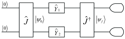
Figure 1: The block diagram for the Eisert’s scheme.

In their model, at first two basis vectors $\{|C=0\rangle,|D=1\rangle\}$ in Hilbert space are assigned to the possible outcomes of the classical strategies, $C=0$ and $D=1$ respectively [23]. Then, suppose the initial state is $|\psi_{0}\rangle=\hat{J}~{}|00\rangle$ before the game is played, where $\hat{J}$ is an entangling operator that is known to both players. For a $2\times 2$ game, the entangling operator $\hat{J}$ has form below [37, 38]

$$\hat{J}(\omega)=\exp(i\frac{\omega}{2}\sigma_{x}^{\otimes 2})=I^{\otimes 2}\cos\frac{\omega}{2}+i\sigma_{x}^{\otimes 2}\sin\frac{\omega}{2}$$ (3)

where $\omega\in[0,\pi/2]$ is a measure of entanglement of a game. When $\omega=\pi/2$, there is a maximally entangled game, in which the entangling operator can be written as

$$\hat{J}(\omega)=\frac{1}{\sqrt{2}}~{}(I^{\otimes 2}+i\sigma_{x}^{\otimes 2}).$$ (4)

Next, each agent chooses a unitary operator $\hat{Y}$ as a strategy from the two-parameter strategy space $\hat{S}$ [23]

$$\hat{Y}(\gamma,\phi)=\begin{pmatrix}e^{i\phi}\cos\frac{\gamma}{2}&\sin\frac{\gamma}{2}\\ -\sin\frac{\gamma}{2}&e^{-i\phi}\cos\frac{\gamma}{2}\end{pmatrix}\in\hat{S},$$ (5)

where $\gamma\in[0,\pi]$, $\phi\in[0,\pi/2]$. Then, she/he operates it on the qubit that belongs to her/him, which makes the game in a state $(\hat{Y_{1}}\otimes\hat{Y_{2}})\hat{J}|00\rangle$. In the end, before a projective measurement on the basis $\{|0\rangle,|1\rangle\}$ is carried out, the final state is

$$|\psi_{f}\rangle=\hat{J}^{{\dagger}}(\hat{Y_{1}}\otimes\hat{Y_{2}})\hat{J}~{}|00\rangle.$$ (6)

As such, the first agent’s expected payoff is written as

$$\Pi(\gamma,\phi)=R|\langle\psi_{f}|00\rangle|^{2}+S|\langle\psi_{f}|01\rangle|^{2}+T|\langle\psi_{f}|10\rangle|^{2}+P|\langle\psi_{f}|11\rangle|^{2}.$$ (7)

3 The Model

Assume there is an undirected network $G(V,E)$ with $N$ nodes, in which $V$ is the set of nodes and $E$ is the set of links. Also, each node $i\in V$ is occupied by an agent and its neighbor $j$ is any other agent such that there is a link between them, so the set of neighbors of an agent $i$ can be defined as $\Gamma_{i}=\{j|e_{ij}\in E,j\in V\backslash i\}$.

In this paper, three different networks will be constructed. They are a Regular Lattice (RL) with periodic boundary conditions, a Newman-Watts (NW) small world network [39, 40] and a Scale-Free (SF) network [41, 42]. When periodic boundary conditions are involved, they can guarantee each node in the regular lattice has four neighbors. In addition, for avoiding isolated nodes, the NW small world network is selected in our work instead of the Watts-Strogatz (WS) network. The NW network can be established in two steps [43]. At first, a regular lattice, with periodic boundary conditions, is constructed, and then links are added with probability $p_{\rm nw}$ between any two randomly chosen nodes. Finally, the SF network is established according to the Barabási-Albert model [41] whose algorithm consists of two steps, growth and preferential attachment. It can start with a small network of $m_{0}\ll N$ all connected nodes, and then a new node with $m\leq m_{0}$ links will be added to the network. Its $m$ links will be connected to $m$ different nodes chosen with probability $p_{\rm sf}(i)$ which can be calculated as below,

$$p_{\rm sf}(i)=\frac{k_{i}}{\sum_{j\in V}k_{j}}.$$ (8)

Here, $k$ is the degree of a node. This procedure will be repeated many times till the number of nodes of the network is $N$.

Initially, each agent on the network is assigned a strategy randomly from the set of strategies $\{\hat{C},\hat{D},\hat{H},\hat{Q}\}$. Next, an agent $i$ will play a $2\times 2$ entangled quantum game in turn with each one of its $|\Gamma_{i}|$ neighbors according to the physical model of a quantum game (Fig. 1), where the symbol $|\cdot|$ is the cardinality of a set. Throughout the paper, all quantum games are maximally entangled games, if not otherwise explicitly stated. And then its expected payoff $\Pi_{ij},j\in\Gamma_{i}$ can be calculated by Eq. 7. The agent’s total payoff $F_{i}$ is obtained by accumulating all it receives $F_{i}=\sum_{j\in\Gamma_{i}}\Pi_{ij}$.

After that, it will choose a neighbor from its neighborhood randomly and imitate its strategy with probability $p_{i}$ [44],

$$p_{i}=\bigg{\{}\begin{array}[]{lll}\frac{F_{j}-F_{i}}{\alpha\cdot\textrm{max}(k_{i},k_{j})},&\textrm{ $F_{j}>F_{i},j\in\Gamma_{i}$}\vspace{4pt}\\ 0,&\textrm{ otherwise}\end{array},$$ (9)

where $\alpha$ is a constant that can be calculated as below according to different games [45],

$$\alpha=\left\{\begin{array}[]{ll}T-S,&\hbox{PD}\vspace{4pt}\\ T-P,&\hbox{SD}\vspace{4pt}\\ R-S,&\hbox{SH}\hskip 4.0pt\textrm{.}\end{array}\right.$$ (10)

After all the agents acquire their payoffs, their strategies are updated synchronously. This process will be repeated by a maximum number of $10^{4}$ generations and the fractions of agents with different strategies are obtained by averaging the last 1000 generations, which produces a result of evolution of strategies. The final result is obtained by averaging over at least 100 of these results. If strategies of all agents do not change for 500 consecutive generations, it is deemed that an equilibrium has been reached and the iterations are stopped.

4 Simulation setup

Assume a population of $50\times 50$ agents are located at nodes of the above mentioned networks. For the NW network, the probability that links are added between any two randomly chosen nodes is $p_{\rm nw}=0.5$, while for the SF network, the number of nodes of the initial core network is $m_{0}=2$ or $3$ and the links of each new node are set at $m=2$. Throughout all simulations, the network topology remains static. In this paper, we consider two sets of strategies:

1. There are three strategies in the set $\hat{S_{1}}=\{\hat{C},\hat{D},\hat{H}\}$. Initially, three strategies, $\hat{C}$ (Cooperation), $\hat{D}$ (Defection), $\hat{H}$ (Hadamard), are assigned to agents randomly and the fractions of strategies are 49%, 50% and 1% respectively. Here, the unitary operators $\hat{C}$ and $\hat{D}$ have the forms below

   $$\hat{C}=\begin{pmatrix}1&0\\ 0&1\end{pmatrix},\hskip 4.0pt\hat{D}=\begin{pmatrix}0&1\\ 1&0\end{pmatrix}.$$ (11)

2. There are four strategies in the set $\hat{S_{2}}=\{\hat{C},\hat{D},\hat{H},\hat{Q}\}$. Initially, four strategies, $\hat{C}$, $\hat{D}$, $\hat{H}$ and $\hat{Q}$, are assigned to the population randomly and the fractions of strategies are 49%, 49%, 1% and 1% respectively. The strategy $\hat{Q}$ takes the form

   $$\hat{Q}=\begin{pmatrix}i&0\\ 0&-i\end{pmatrix}.$$ (12)

In these two cases, the quantum strategy $\hat{H}$ brings a miracle move [23] when an agent uses it against the other’s classical strategy. Also, the quantum strategy profile $(\hat{Q},\hat{Q})$ is a new NE observed by Eisert et al. [23], when players choose their strategies from the strategy space $\hat{S}=\hat{Y}(\gamma,\phi)$.

Then, the PD, SD and SH games are played by all agents on RL, NW, and SF networks respectively. To be compatible with previous studies and without loss of generality, the payoff matrix of the PD game is chosen as $R=1$ (Reward), $T=b$ ($1<b\leq 2$) (Temptation), $P=0$ (Punishment) and $S=0$ (Sucker’s payoff) satisfying the inequalities $T>R>P>S$; the payoff matrix of the SD game as $T=b>1$, $R=b-c/2$, $S=b-c$ and $P=0$ satisfying $T>R>S>P$, and the cost-to-benefit ratio of mutual cooperation is defined as $r=c/(2b-c)$ [14], where $c=1$ and $0<r\leq 1$; the payoff matrix of the SH game as $R=1$, $T=r$ ($0<r\leq 1$), $S=-r$ and $P=0$ satisfying $R>T>P>S$.

The payoffs under any strategy profiles can be calculated according to the model of a quantum game in Section 2. As is known, the strategy profiles $(\hat{H},\hat{H})$ and $(\hat{Q},\hat{Q})$ are Nash equilibria for PD, SD and SH games in Case 1 and Case 2 respectively. However, it is worth noting that for the SH game there are two Nash equilibria, i.e., besides $(\hat{H},\hat{H})$ or $(\hat{Q},\hat{Q})$, the other is $(\hat{C},\hat{C})$.

5 Results and Discussion

Throughout all simulations, the agents with quantum strategies $\hat{H}$ and $\hat{Q}$ are regarded as invaders, so their fractions are restricted to 1% of the whole population initially. Thus, our simulations focus on investigating how the quantum strategies invade the population and how strategies evolve on networks. In order to elucidate the affects of quantum strategies, three games are considered to observe the behavior of quantum strategies. Furthermore, the structure of a network is also a key factor for the evolution of strategies, so three different networks (RL, NW and SF) are constructed to test their influences.

For Case 1, the upper and median sub-figures of Fig. 2 show that the fractions of agents with three strategies on RL and NW networks are similar. Given our three games, the quantum strategy $\hat{H}$ becomes the Evolutionarily Stable Strategy (ESS) almost from the outset when the PD game is played, i.e., even if the temptation $T$ is only a little larger than the reward $R$, the strategy $\hat{H}$ can dominate the network successfully. However, for SD and SH games, it is more difficult for the strategy $\hat{H}$ to be the ESS. When the SD game is employed, the strategy $\hat{H}$ is played by all agents on the network, only if the cost-to-benefit ratio $r\geq 0.32$ and $r\geq 0.40$ on RL and NW networks respectively. Before this value, almost no agents use the strategy $\hat{H}$, while at that time the frequencies of the strategies $\hat{C}$ and $\hat{D}$ are similar to the case of a SD game without a quantum strategy. For the SH game, a coordination game, the strategy $\hat{H}$ invades the network successfully when $r\geq 0.82$ and $r\geq 0.67$ respectively on RL and NW networks. From above analysis, it can be said that the SH game and the structure of NW network is more advantageous for classical strategies than the quantum ones.

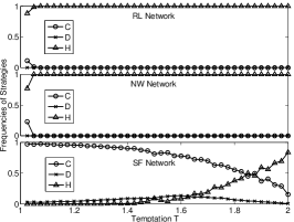
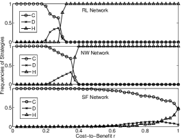
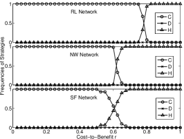
Figure 2: Fractions of agents with three strategies in Case 1 on different games and networks. (a) Prisoners’ Dilemma. (b) Snowdrift. (c) Stag-Hunt. In the upper, median and lower sub-figures of (a),(b) and (c), games are played on RL, NW and SF networks respectively.

The results of evolution of strategies in Case 2 are shown in Fig. 3. From Fig. 3, it can be seen that for the PD the strategy $\hat{Q}$ can invade the whole network from the outset on both the RL and NW networks, and the strategy $\hat{Q}$ becomes the dominate strategy over $\hat{H}$ in Case 1 when the SD and SH games are adopted, which is improved about 10%, 8% (SD on RL and NW) and 30%, 15% (SH on RL and NW) respectively. In contrast to Case 1, it can be inferred that the strategy $\hat{Q}$ is more aggressive than the strategy $\hat{H}$.

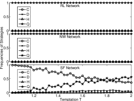
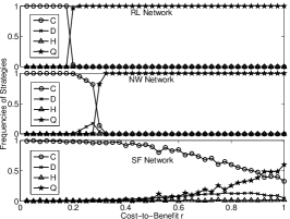
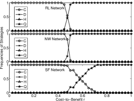
Figure 3: Fractions of agents with four strategies in Case 2 on different games and networks. (a) Prisoners’ Dilemma. (b) Snowdrift. (c) Stag-Hunt. In the upper, median and lower sub-figures of (a),(b) and (c), games are played on RL, NW and SF networks respectively.

On the other hand, the evolution of strategies on the SF network is more complex due to the features of the SF network, i.e., the power-law distribution of degrees of nodes in the network. In both Case 1 and 2, all strategies fluctuate no matter which game is played. However, it can be observed that the classical strategies decrease in proportion with the increase of the variable $T$ or $r$, while the quantum strategies act conversely. According to the features of the SF network, if few quantum strategies are played by some agents with small degrees, it will be harder for them to invade the network. This raises the question that if a quantum strategy is employed by a certain agent with one of the first three largest degrees, namely a hub node, how will the quantum strategies evolve? In the next simulations, the agent with the first largest degree will be compulsorily assigned a strategy $\hat{H}$ in Case 1 or $\hat{Q}$ in Case 2 after each agent chooses a strategy. The results are shown in the uppermost sub-figure in Fig. 4 and Fig. 5, while the other two sub-figures in Fig. 4 and Fig. 5 are the results when the agent with the second or the third largest degree plays a strategy $\hat{H}$ or $\hat{Q}$. This procedure is applied on the PD, SD and SH games, respectively.

From Fig. 4 and Fig. 5, it can be seen that when the agent with the first largest degree plays a quantum strategy, the fluctuations in the results reduce significantly, which means that if the node with the largest degree is occupied by an agent with a quantum strategy, then the strategy spreads out more quickly on the SF network and the population is invaded more easily by the strategy. If the quantum strategy is assigned to an agent with the second or the third largest degree, the fluctuations also decrease, but it is not lower than that of the first one. As for the three games, the SH game makes the fluctuations of results lower than those on the PD and SD games regardless of degrees. Furthermore, comparing the two strategies $\hat{H}$ and $\hat{Q}$, we can find that the value of the temptation $T$ or the cost-to-benefit $r$ when the strategy $\hat{Q}$ becomes dominated is smaller than that of the strategy $\hat{H}$ according to Fig. 4 and Fig. 5.

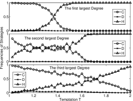
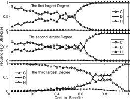
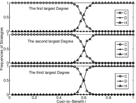
Figure 4: Fractions of agents with different strategies in Case 1 on a SF network, when the agents with the first three largest degrees play the quantum strategy $\hat{H}$. (a) Prisoners’ Dilemma. (b) Snowdrift. (c) Stag-Hunt. In the upper, median and lower sub-figures of (a),(b) and (c), the agent with the first, second or third degree is assigned the quantum strategy $\hat{H}$ respectively.

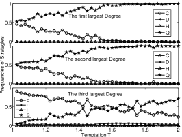
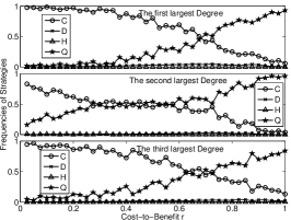
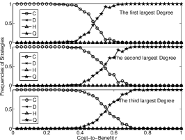
Figure 5: Fractions of agents with different strategies in Case 2 on a SF network, when the agents with the first three largest degrees play the quantum strategy $\hat{Q}$. (a) Prisoners’ Dilemma. (b) Snowdrift. (c) Stag-Hunt. In the upper, median and lower sub-figures of (a),(b) and (c), the agent with the first, second or third degree is assigned the quantum strategy $\hat{Q}$ respectively.

For Case 2, the main reason why quantum strategies do not invade the population from the outset is that initially the fractions of agents with quantum strategies are too low. If the fraction is increased, the quantum strategy $\hat{Q}$ will be able to dominate the network. In simulations, the fractions of the strategy $\hat{D}$ and $\hat{H}$ remain constant at 49% and 1%, while the fractions of the other two strategies are adjusted. Further, the fraction of the quantum strategy $\hat{Q}$ is set at 10%, 20% and 25% respectively and correspondingly the fraction of the strategy $\hat{C}$ is 40%, 30% and 25%. For the SF network, the agent occupying the node with the largest degree is assigned a quantum strategy. Fig. 6 exhibits the evolution of strategies when the fraction of the quantum strategy $\hat{Q}$ is 25%, where we can see that the quantum strategy $\hat{Q}$ can invade the population successfully on all networks and becomes the ESS from the outset.

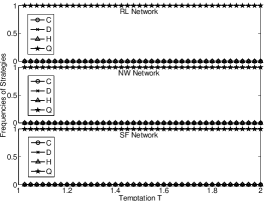
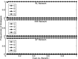
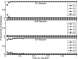
Figure 6: Fractions of agents with different strategies in Case 2 on three games and three networks, when the fraction of the quantum strategy $\hat{Q}$ is increased at 25%. (a) Prisoners’ Dilemma. (b) Snowdrift. (c) Stag-Hunt. In the upper, median and lower sub-figures of (a),(b) and (c), games are played on RL, NW and SF networks respectively.

However, for Case 1, the situation is more complex than that in Case 2. Besides the reason mentioned above, another major reason also prevents the quantum strategy $\hat{H}$ being spread on networks that is the strategy profile $(\hat{H},\hat{H})$ is not Pareto optimal although it is a Nash equilibrium. Hence, even if the fraction of the quantum strategy $\hat{H}$ is increased to 25%, it cannot dominate on all networks from the outset, especially on the SF network, as is shown in Fig. 7, in which similarly the fraction of the quantum strategy $\hat{H}$ is set at 25% and correspondingly the fraction of the strategy $\hat{C}$ is also 25%, while the fraction of the strategy $\hat{D}$ remains constantly at 50%.

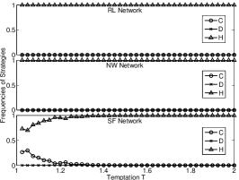
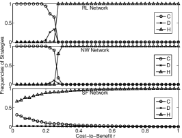
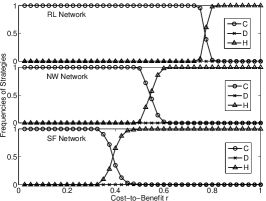
Figure 7: Fractions of agents with different strategies in Case 1 on three games and three networks, when the fraction of the quantum strategy $\hat{H}$ is increased at 25%. (a) Prisoners’ Dilemma. (b) Snowdrift. (c) Stag-Hunt. In the upper, median and lower sub-figures of (a),(b) and (c), games are played on RL, NW and SF networks respectively.

6 Conclusions

In summary, we investigate the evolution of strategies on networks when quantum strategies $\hat{H}$ and $\hat{Q}$ are employed as invaders. For the evolution of strategies, the structure of a network is a decisive factor and a game represents an agent’s response to some external stimuli. So, we construct three networks and introduce three games in this paper to investigate the evolution of strategies on these networks in a defector dominated population when different games are employed. As far as two quantum strategies are concerned, the strategy $\hat{Q}$ is more aggressive than the other one regardless of Case 1 or Case 2, because it is not only a Nash equilibrium but also Pareto optimal. Considering three networks, we find that the population on a RL network can be invaded most easily by quantum strategies without any small world effects (properties), namely short average path length and large clustering coefficient. On the contrary, in the SF network the power-law distribution of degrees makes the spread of quantum strategies more difficult and exacerbates the fluctuations of results when few quantum strategies happen to be played by some agents only with small degrees. If an agent with a quantum strategy occupies a hub, i.e. a node with the largest degree, the fluctuations reduce considerably. Furthermore, if the fractions of quantum strategies are increased significantly, they can dominate a network from the outset.

References

- Nowak and May [1992] M. A. Nowak, R. M. May, Nature 359 (1992) 826–829.
- Nowak and May [1993] M. A. Nowak, R. M. May, International Journal of Bifurcation and Chaos 3 (1993) 35–78.
- Szolnoki et al. [2009] A. Szolnoki, M. Perc, G. Szabó, H.-U. Stark, Physical Review E 80 (2009) 021901.
- Szabó et al. [2009] G. Szabó, A. Szolnoki, J. Vukov, Europhysics Letters 87 (2009) 18007.
- Perc and Szolnoki [2010] M. Perc, A. Szolnoki, Biosystems 99 (2010) 109–125.
- Shang et al. [2006] L. H. Shang, X. Li, X. F. Wang, European Physical Journal B 54 (2006) 369–373.
- Wu and Wang [2007] Z.-X. Wu, Y.-H. Wang, Physical review. E 75 (2007) 041114.
- Chen and Wang [2008] X. Chen, L. Wang, Physical Review E 77 (2008) 017103.
- Assenza et al. [2008] S. Assenza, J. Gomez-Gardenes, V. Latora, Physical Review E 78 (2008) 017101.
- Lee et al. [2008] K. H. Lee, C.-H. Chan, P. M. Hui, D.-F. Zheng, Physica a-Statistical Mechanics and Its Applications 387 (2008) 5602–5608.
- Perc [2009] M. Perc, New Journal of Physics 11 (2009) 033027.
- Taylor and Jonker [1978] P. Taylor, L. Jonker, Mathematical Biosciences 40 (1978) 145–156.
- Skyrms [2004] B. Skyrms, Stag-Hunt Game and the Evolution of Social Structure, Cambridge University Press, Cambridge, UK, 2004.
- Hauert and Doebeli [2004] C. Hauert, M. Doebeli, Nature 428 (2004) 643–646.
- Szolnoki et al. [2009] A. Szolnoki, M. Perc, G. Szabó, Physical Review E 80 (2009) 056109.
- Helbing et al. [2010] D. Helbing, A. Szolnoki, M. Perc, G. Szabó, New Journal of Physics 12 (2010) 083005.
- Starnini et al. [2011] M. Starnini, A. Sanchez, J. Poncela, Y. Moreno, Journal of Statistical Mechanics-Theory and Experiment 2011 (2011) P05008.
- Turner and Chao [1999] P. E. Turner, L. Chao, Nature 398 (1999) 441–443.
- Pfeiffer et al. [2001] T. Pfeiffer, S. Schuster, S. Bonhoeffer, Science 292 (2001) 504–507.
- Frick and Schuster [2003] T. Frick, S. Schuster, Naturwissenschaften 90 (2003) 327–331.
- Chettaoui et al. [2007] C. Chettaoui, F. Delaplace, M. Manceny, M. Malo, Biosystems 87 (2007) 136–141.
- Meyer [1999] D. A. Meyer, Physical Review Letters 82 (1999) 1052.
- Eisert et al. [1999] J. Eisert, M. Wilkens, M. Lewenstein, Physical Review Letters 83 (1999) 3077.
- Marinatto and Weber [2000] L. Marinatto, T. Weber, Physics Letters A 272 (2000) 291–303.
- Iqbal and Toor [2001] A. Iqbal, A. H. Toor, Physics Letters A 280 (2001) 249–256.
- Kay et al. [2001] R. Kay, N. F. Johnson, S. C. Benjamin, Journal of Physics A: Mathematical and General 34 (2001) L547–L552.
- Du et al. [2002] J. Du, H. Li, X. Xu, M. Shi, J. Wu, X. Zhou, R. Han, Physical Review Letters 88 (2002) 137902.
- Prevedel et al. [2007] R. Prevedel, A. Stefanov, P. Walther, A. Zeilinger, New Journal of Physics 5 (2007) 205–215.
- Schmid et al. [2009] C. Schmid, A. P. Flitney, W. Wieczorek, N. Kiesel, H. Weinfurter, L. C. L. Hollenberg, arXiv:0901.0063v1 (2009).
- Flitney and Abbott [2002] A. P. Flitney, D. Abbott, Fluctuation & Noise Letters 2 (2002) R175–R188.
- Guo et al. [2008] H. Guo, J. Zhang, G. J. Koehler, Decision Support Systems 46 (2008) 318–332.
- Ekert et al. [2001] A. Ekert, P. M. Hayden, H. Inamori, Coherent atomic matter waves 72 (2001) 661–702.
- Nielsen and Chuang [2000] M. A. Nielsen, I. L. Chuang, Quantum Computation and Quantum Information, Cambridge University Press, Cambridge, 2000.
- Nash [1950] J. Nash, Proceedings of the National Academy of Sciences 36 (1950) 48–49.
- Nash [1951] J. Nash, The Annals of Mathematics 54 (1951) 286–295.
- Fudenberg and Tirole [1983] D. Fudenberg, J. Tirole, Game Theory, MIT Press, 1983.
- Benjamin and Hayden [2001] S. C. Benjamin, P. M. Hayden, Physical Review A 64 (2001) 030301.
- Du et al. [2001] J. Du, H. Li, X. Xu, M. Shi, X. Zhou, R. Han, Arxiv preprint quant-ph/0111138 (2001).
- Newman and Watts [1999a] M. E. J. Newman, D. J. Watts, Physical Review E 60 (1999a) 7332.
- Newman and Watts [1999b] M. E. J. Newman, D. J. Watts, Physics Letters A 263 (1999b) 341–346.
- Barabási and Albert [1999] A.-L. Barabási, R. Albert, Science 286 (1999) 509–512.
- Albert and Barabási [2002] R. Albert, A.-L. Barabási, Reviews of Modern Physics 74 (2002) 47.
- Newman [2003] M. E. J. Newman, SIAM Review 45 (2003) 167–256.
- Santos et al. [2005] F. C. Santos, J. F. Rodrigues, J. M. Pacheco, Physical Review E 72 (2005) 056128.
- Szabó and Fath [2007] G. Szabó, G. Fath, Physics Reports-Review Section of Physics Letters 446 (2007) 97–216.