Holographic RG flows and transport coefficients in Einstein-Gauss-Bonnet-Maxwell theory 

Abstract

We apply the membrane paradigm and the holographic Wilsonian approach to the Einstein-Gauss-Bonnet-Maxwell theory. The transport coefficients for a quark-gluon plasma living on the cutoff surface are derived in a spacetime of charged black brane. Because of the mixing of the Gauss-Bonnet coupling and the Maxwell fields, the vector modes/shear modes of the metric and Maxwell fluctuations turn out to be very difficult to decouple. We firstly evaluate the AC conductivity at a finite cutoff surface by solving the equation of motion numerically, then manage to derive the radial flow of DC conductivity with the use of the Kubo formula. It turns out that our analytical results match the numerical data in low frequency limit very well. The diffusion constant $D(u_{c})$ is also derived in a long wavelength expansion limit. We find it depends on the Gauss-Bonnet coupling as well as the position of the cutoff surface.

1 Introduction

Recently, a holographic version of Wilsonian renormalization group (hWRG) has been proposed to describe field theories with a finite cut-off [1, 2, 3, 4]. The essential idea of hWRG is to integrate out the bulk field from the boundary up to some intermediate radial distance. The radial direction in the bulk marks the energy scale of the boundary theory and the radial flow in the bulk geometry can be interpreted as the renormalization group flow of the boundary theory[5, 6, 7, 8, 9, 10, 11, 12, 13, 14, 15]. Moreover, some evidence has been presented in [16] indicating that the membrane paradigm and the hWRG method are probably equivalent.

In [3] and later in [17], it was shown that the diffusion coefficient for Reissner-Nordstrom-Anti de Sitter(RN-AdS) black holes can be calculated in the scaling limit without explicit decoupling procedure. In [17], the authors discussed the mixing effect between metric fluctuation and Maxwell fluctuation in RN-AdS spacetime. They firstly derived the diffusion constant through the mixed RG flow equations, and then turn to the standard hydrodynamic calculation on the cut-off surface by decoupling the equations of motion. It was found that the results through the RG flow approach match those through the hydrodynamic calculation in good agreements.

In this paper, we intend to apply these approaches to investigate the vector-type fluctuations in Einstein-Gauss-Bonnet-Maxwell theory. So far, the diffusion coefficient for charged black holes in this theory has not been computed in the previous literature. It is also interesting to study the electric conductivity, charge susceptibility and thermal conductivity of the dual fluid in this theory. Unlike the RN-AdS spacetime, the equations of motion, followed the method given in [18, 19], are essentially failed to be decoupled because of the mixing of the Gauss-Bonnet coupling and the charge. Nevertheless, in this paper we intend to disclose one advantage of the membrane paradigm and the hWRG approach, which tell us that even the equations of motion can not be decoupled, one can still calculate the transport coefficients analytically. We will generalize the strategy presented in [3] to calculate the cutoff-dependent diffusion constant $D(u_{c})$ when the Gauss-Bonnet terms are involved. We will also investigate the DC conductivity at an arbitrary radius by using the Kubo formula without obtaining the decoupled matter equations as in [17]. The charge susceptibility and the thermal conductivity are also evaluated. It was suggested in [20] that the ratio of the conductivity to the susceptibility may obey a universal bound. In [21], it was shown that this bound is violated in the framework of general four-derivative interactions. We will extend this discussion in the Gauss-Bonnet gravity in this paper as well.

This paper is organized as follows. In section 2, we present our basic setup for the vector type perturbation following the notation in [22]. We define the effective “current” and “strength” for the perturbation fields, and then rewrite the equations of motion in a form similar to the Maxwell equation. In section 3, we first investigate the AC conductivity of the dual plasma with the use of the numerical analysis. Then we study the DC conductivity flow at an arbitrary radius through the Kubo formula. Following the method developed in [2, 3, 17], we calculate the diffusion constant in the scaling limit. The resulting formula for the diffusion constant reproduces the old result from the membrane paradigm in the absence of the Gauss-Bonnet coupling. We then provide a consistent check on the obtained diffusion constant by employing the Brown-York tensor on the cutoff surface. Conclusion and discussion are presented in section 4. We also show in the appendix the full equations of motions for vector type perturbations.

2 Basic setup

We start by introducing the following action in $D$ dimensions which includes Gauss-Bonnet terms and $U(1)$ gauge field:

$$I=\frac{1}{2\kappa^{2}}\!\int\!{\rm d}^{D}\!x\sqrt{-g}\Big{(}R-2\Lambda+\tilde{\alpha}\left(R_{\mu\nu\rho\sigma}R^{\mu\nu\rho\sigma}-4R_{\mu\nu}R^{\mu\nu}+R^{2}\right)-\frac{4\pi G_{D}}{g^{2}}F_{\mu\nu}F^{\mu\nu}\Big{)},$$ (2.1)

where $2\kappa^{2}=16\pi G_{D}$, $g^{2}$ the $D$-dimensional gauge coupling constant, and $\tilde{\alpha}$ is a Gauss-Bonnet coupling constant with dimension $\rm(length)^{2}$. The field strength is defined as $F_{\mu\nu}(x)=\partial_{\mu}A_{\nu}(x)-\partial_{\nu}A_{\mu}(x)$. The corresponding Einstein equation reads as

$$R_{\mu\nu}-\frac{1}{2}g_{\mu\nu}R+g_{\mu\nu}\Lambda=\frac{8\pi G_{D}}{g^{2}}\Big{(}F_{\mu\rho}F_{\nu\sigma}g^{\rho\sigma}-\frac{1}{4}g_{\mu\nu}F_{\rho\sigma}F^{\rho\sigma}\Big{)}+T^{\rm eff}_{\mu\nu},$$ (2.2)

where

$$T^{\rm eff}_{\mu\nu}=\tilde{\alpha}\Bigg{[} \frac{1}{2}g_{\mu\nu}\Big{(}R_{\alpha\beta\rho\sigma}R^{\alpha\beta\rho\sigma}-4R_{\alpha\beta}R^{\alpha\beta}+R^{2}\Big{)}-2RR_{\mu\nu}+4R_{\mu\rho}R_{\nu}{}^{\rho}$$ (2.3)

$$+4R_{\rho\sigma}R_{\mu\nu}{}^{\rho\sigma}-2R_{\mu\rho\sigma\gamma}R_{\nu}{}^{\rho\sigma\gamma}\Bigg{]}.$$

The charged black brane/hole solution to this equation in $D$ dimensions is described by [23, 24, 25]

$${\rm d}s^{2} = -g_{tt}dt^{2}+g_{rr}dr^{2}+g_{ii}{\rm d}x^{i}{\rm d}x^{i}$$ (2.4)

$$= \displaystyle-H(r)N^{2}{\rm d}t^{2}+H^{-1}(r){\rm d}r^{2}+\frac{r^{2}}{l^{2}}{\rm d}x^{i}{\rm d}x^{i},$$

$$A_{t} = \displaystyle\mu\bigg{(}1-\frac{r^{D-3}_{+}}{r^{D-3}}\bigg{)},$$ (2.5)

with

$$H(r) = k_{0}+\frac{r^{2}}{2\lambda l^{2}}\left[1-\sqrt{1-4\lambda\bigg{(}1-\frac{r^{D-1}_{+}}{r^{D-1}}-a\frac{r^{D-1}_{+}}{r^{D-1}}+a\frac{r^{2D-4}_{+}}{r^{2D-4}}\bigg{)}}\right],$$ (2.6)

$$\Lambda = -\frac{(D-1)(D-2)}{2l^{2}},$$ (2.7)

where $\tilde{\alpha}$, $\alpha$ and $\lambda$ are related by $\alpha=(D-4)(D-3)\tilde{\alpha}$, and $\lambda=\alpha/l^{2}$, $a=\frac{l^{2}\kappa^{2}}{(D-2)(D-3)g^{2}}Q^{2}$ with the parameter $l$ corresponding to AdS radius. The chemical potential $\mu$ is related to $Q$ by $Q=\frac{\mu(D-3)}{r_{+}}$ and the horizon $r_{+}$ is the largest root of $H(r)=0$. The charge density evaluated at the asymptotic boundary is $n_{q}=\frac{Qr^{3}_{+}}{g^{2}l^{3}}$.

The constant $N^{2}$ in the metric (2.4) can be fixed by requiring that the geometry of the spacetime should asymptotically approach to the conformaly flat metric at spatial infinity, i.e. ${\rm d}s^{2}\propto-c^{2}{\rm d}t^{2}+{\rm d}\vec{x}^{2}$. Since as $r\rightarrow\infty$, we have

$$H(r)N^{2}\rightarrow\frac{r^{2}}{l^{2}},$$

one can find $N^{2}$ to be

$$N^{2}=\frac{1}{2}\Big{(}1+\sqrt{1-4\lambda}\ \Big{)}.$$ (2.8)

Without loss of generality, in the following of this paper we will mainly focus on five-dimensional case $D=5$ with $k_{0}=0$. After introducing the coordinate as follows

$$u=\frac{r^{2}_{+}}{r^{2}},~{}~{}H(u)=\frac{r^{2}_{+}}{ul^{2}}f(u),~{}~{}f(u)=\frac{1}{2\lambda}\bigg{(}1-\sqrt{1-4\lambda(1-u)(1+u-au^{2})}\bigg{)},$$ (2.9)

the metric can be rewritten as

$$ds^{2}=\frac{r^{2}_{+}}{l^{2}}\frac{1}{u}\bigg{(}-f(u)N^{2}dt^{2}+\sum^{3}_{i=1}dx^{i}dx^{i}\bigg{)}+\frac{l^{2}}{4u^{2}}\frac{du^{2}}{f(u)}.$$ (2.10)

The Hawking temperature of the black brane can be worked out as

$$T_{H}=\frac{Nr_{+}}{2\pi l^{2}}(2-a).$$ (2.11)

We follow the notation in [22] hereafter and note that a rotational symmetry among $x^{i}$ directions, i.e. $g_{ij}=g_{xx}\delta_{ij}$ with $x$ being one of the spatial direction.

The shear modes of the metric perturbations $h_{xz}$, $h_{xt}$, $h_{xr}$ exhibit the same behavior as the Maxwell field $a_{z}$, $a_{t}$ and $a_{r}$, thus we can define

$$a_{z}\equiv h^{x}_{z},~{}~{}~{}a_{t}\equiv h^{x}_{t},~{}~{}~{}a_{u}\equiv h^{x}_{u}.$$ (2.12)

Note that in the gauge $a_{u}=0$, $a_{t}$ and $a_{z}$ decouple from the other components. It turns out that the vector part of the off shell action for the shear modes in charged Gauss-Bonnet gravity is given by

$$S=\int d^{5}x\sqrt{-g}\bigg{[}-\frac{1}{4g^{2}}F^{\mu\nu}F_{\mu\nu}-\frac{1}{4g^{2}_{eff}(r)}\bigg{(}{f}^{ut}{f}_{ut}+\tilde{f}^{uz}\tilde{f}_{uz}+\tilde{f}^{zt}\tilde{f}_{zt}\bigg{)}+\frac{1}{g^{2}}\frac{4u^{3}}{r^{2}_{+}}a_{t}A^{\prime}_{x}A^{\prime}_{t}\bigg{]}.$$ (2.13)

Let us define the effective “current” and “strength” for the $a_{\mu}$ as

$$j^{t}=\frac{1}{g^{2}_{eff}(r)}\sqrt{-g}\mathcal{M}uf^{ut},~{}~{}~{}j^{z}=-\frac{1}{g^{2}_{eff}(r)}\sqrt{-g}\tilde{f}^{uz},$$ (2.15)

$$f_{ut}=\partial_{u}a_{t}-\partial_{t}a_{u},$$

$$\tilde{f}_{uz}=-u^{2}\mathcal{M}^{\prime}{f}_{uz}=-u^{2}\mathcal{M}^{\prime}(\partial_{u}a_{z}-\partial_{z}a_{u}),$$ (2.17)

$$\tilde{f}_{zt}=-u^{2}\mathcal{M}^{\prime}{f}_{zt}=-u^{2}\mathcal{M}^{\prime}(\partial_{z}a_{t}-\partial_{t}a_{z}),$$

where $\mathcal{M}=\frac{1-2\lambda f}{u}$ and the prime ^′ denotes the derivative with respect to $u$. $j^{\mu}$ is the conjugate momentum of the field $a^{\mu}$. Because of the presence of the Gauss-Bonnet terms, the definition of the effective current and strength becomes a little bit complicated than that of the Einstein case[17] and it can return to the Einstein case without the Gauss-Bonnet terms. For chargeless Gauss-Bonnet black branes, the equations of motion can be written as

$$\partial_{t}j^{t}+\partial_{z}j^{z}=0,$$ (2.18)

$$\partial_{u}j^{t}+Gg^{tt}g^{zz}\partial_{z}\tilde{f}_{zt}=0,$$ (2.19)

$$\partial_{u}j^{z}-Gg^{tt}g^{zz}\partial_{z}\tilde{f}_{zt}=0,$$ (2.20)

where we have used the notations

$$G=\sqrt{-g}/g^{2}_{eff}(r)=\frac{r^{6}_{+}N}{4\kappa^{2}u^{4}l^{5}},~{}~{}~{}\frac{1}{g^{2}_{eff}(r)}=\frac{r^{2}_{+}}{2\kappa^{2}l^{2}u}.$$ (2.21)

For the charged black brane there is a matter perturbation $A_{x}$, and in this case we may define the charge density as

$$\tilde{j}^{t}={j}^{t}-\frac{1}{g^{2}}\sqrt{-g}\frac{4u^{3}}{r^{2}_{+}}A^{\prime}_{t}A_{x}.$$ (2.22)

The equations of motion then take the following form

$$\partial_{t}\tilde{j}^{t}+\partial_{z}j^{z} = 0,$$ (2.23)

$$\partial_{u}\tilde{j}^{t}+Gg^{tt}g^{zz}\partial_{z}\tilde{f}_{zt} = 0,$$ (2.24)

$$\partial_{u}j^{z}-Gg^{tt}g^{zz}\partial_{t}\tilde{f}_{zt} = 0.$$ (2.25)

The Bianchi identity yields

$$\partial_{u}\bigg{(}\frac{\tilde{f}_{zt}}{-u^{2}\mathcal{M}^{\prime}}\bigg{)}-\frac{g_{uu}g_{tt}\partial_{z}j^{t}}{u\mathcal{M}G}+\frac{\partial_{t}j_{z}}{u^{2}\mathcal{M}^{\prime}G}=0.$$ (2.26)

The equation of motion for $A_{x}$ can be written as

$$\partial_{u}\tilde{J}^{x}-\frac{1}{g^{2}N^{2}}g^{xx}\bigg{(}-g^{tt}N^{2}\partial_{t}F_{tx}+g^{zz}\partial_{z}F_{zx}\bigg{)}=0,$$ (2.27)

where the current $\tilde{J}^{x}$ containing the mixed term is defined as

$$\tilde{J}^{x}=J^{x}+\frac{1}{g^{2}}\sqrt{-g}\frac{4u^{3}}{r^{2}_{+}N^{2}}A^{\prime}_{t}a_{t},~{}~{}~{}J^{x}=-\frac{1}{g^{2}}\sqrt{-g}g^{uu}g^{xx}\partial_{u}A_{x}.$$ (2.28)

Here $F_{\mu\nu}$ characterize the strength of the Maxwell fields $A_{\mu}$ and should not be confused with the effective strength of the vector modes of gravity $f_{\mu\nu}$. The matter perturbation $A_{x}$ is also constrained by the Bianchi identity

$$\partial_{u}F_{xt}-\frac{g^{2}g_{uu}g_{xx}}{\sqrt{-g}}\partial_{t}J^{x}=0,$$ (2.29)

$$\partial_{z}F_{tx}+\partial_{t}F_{xz}=0.$$ (2.30)

3 Transport coefficients

In this section, we will evaluate the transport coefficients of the dual plasma on the cutoff surface by solving the equations of motion for charged black holes. We will first compute the AC conductivity numerically and then derive the DC conductivity by using the Kubo formula. We derive the cutoff dependent diffusion constant in the scaling limit. Finally, we provide a consistent check on the obtained diffusion constant.

3.1 AC electric conductivity flow at $k_{z}=0$

We will work in Fourier space. For instance, we expand $a_{z}$ as

$$a_{z}(t,z,u)=\int\frac{d^{4}k}{(2\pi)^{4}}e^{-i\omega t+ikz}a_{z}(k,u).$$ (3.1)

The same decomposition is applicable to $a_{t}$ and $A_{x}$. In the zero momentum limit, $A_{x}$ decouples from $a_{t}$

$$\partial_{u}\bigg{(}\sqrt{-g}g^{uu}g^{xx}\partial_{u}A_{x}\bigg{)}-\frac{g^{2}_{eff}}{g^{2}}\sqrt{-g}(A^{\prime}_{t})^{2}\frac{4u^{2}}{\mathcal{M}r^{2}_{+}}A_{x}+\omega^{2}\sqrt{-g}g^{xx}g^{tt}A_{x}=0.$$ (3.2)

The on-shell action for $A_{x}$ at the cut-off surface $u=u_{c}$ is given by

$$S=\int\tilde{J}^{x}A_{x}.$$ (3.3)

The electric conductivity of the plasma on this cut-off surface can be defined as

$$\sigma_{A}(\omega,u_{c})=\frac{J^{x}}{i\omega A_{x}}.$$ (3.4)

Then equation (3.2) can be recast as

$$\frac{\partial_{u_{c}}\sigma_{A}}{i\omega}-\frac{g^{2}\sigma^{2}_{A}}{\sqrt{-g}g^{uu}g^{xx}}-\frac{g^{2}_{eff}\sqrt{-g}}{g^{4}\omega^{2}}(A^{\prime}_{t})^{2}\frac{4u^{2}}{\mathcal{M}r^{2}_{+}}+\frac{1}{g^{2}}\sqrt{-g}g^{xx}g^{tt}=0.$$ (3.5)

The regularity condition on the horizon gives

$$\sigma_{A}(u=1)=\frac{1}{g^{2}}\frac{r_{+}}{l},$$ (3.6)

in agreement with the result given in [22]. It is worth noting that the conductivity at the event horizon neither depends on the charge, nor the Gauss-Bonnet coupling. In other words, we can say the regularity at the horizon corresponding to setting

$$J^{x}(1)=i\omega\sigma_{A}(1)A_{x}(1)=i\omega\frac{1}{g^{2}}\sqrt{\frac{-g}{g_{uu}g_{tt}}}g^{xx}\bigg{|}_{u=1}A_{x}(1).$$ (3.7)

This relation is useful in determining the DC conductivity.

In order to have an explicit picture on the solutions of conductivity, we solve equation (3.5) numerically and plot the conductivity flows with different charges in Figure 1. From this figure, we can see that when the charged black brane becomes extremal, there is a fixed point for the flow of conductivity near the horizon due to the appearance of $\rm AdS_{2}$ near the horizon. Same as [17], this fixed point will disappear in non-extremal case. The numerical calculation also implies that as $\omega$ approaches to zero, the real part of the conductivity behaves more like equation (3.22). The numerical results in Figure 1 change little for different values of Gauss-Bonnet coupling.

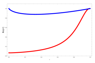
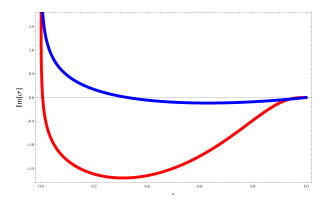
Figure 1: The radial flow of AC conductivity in five-dimensional RN-AdS-Gauss-Bonnet black holes for non-extremal case (blue line) and extremal case (red line) from up to bottom. Here we set $\lambda=0.01$, $r_{+}=1$, $\mu=0.1$, $g=l=G_{5}=1$ and $\omega=0.978$ for the non-extremal case, but $a=2$ for the extremal case.

3.2 DC conductivity flow

We now turn to the DC conductivity in the perturbative background. The conductivity can be evaluated by using the Kubo formula, which relates the conductivity to the low frequency and zero momentum limit of the retarded Green’s function [26, 27]

$$G^{R}_{x,x}(\omega,k=0)=-i\int dtd\textbf{x}e^{i\omega t}\theta(t)<[J_{x}(x),J_{x}(0)]>,$$ (3.8)

where $J_{\mu}$ is the conformal field theory (CFT) current dual to the bulk gauge field $A_{\mu}$. The DC conductivity is given by

$$\sigma_{DC}=-\lim_{\omega\rightarrow 0}\frac{e^{2}{\rm Im}G^{R}_{x,x}(\omega,k=0)}{\omega}.$$ (3.9)

According to [20], the constant $e$ marks the coupling between the boundary current and an external or auxiliary vector field. To the leading order of $e$, the effects of the auxiliary vector are negligible and the conductivity can be fixed from the original CFT. In the absence of chemical potential the general form of conductivity was derived in [22] through the membrane paradigm. But when the chemical potential is taken into account, those formulae need revision as there is a non-trivial flow from horizon to boundary. At the linear level of equations and in the zero momentum limit metric perturbation $a_{z}$ decouples from the rest (see the Appendix for more details). The corresponding component of Einstein’s equations becomes a constraint

$${a_{t}}^{\prime}=\frac{3aN^{2}B(u)}{\mathcal{M}},$$ (3.10)

where $B$ is defined as $B=\frac{A_{x}}{\mu}=\frac{2A_{x}}{Qr_{+}}$. Equation (3.10) can also be obtained in the scaling limit $\omega\sim k^{2}\ll 1$. After substitution one finds the equation for perturbed gauge fields to be

$$B^{\prime\prime}+\frac{f^{\prime}}{f}B^{\prime}+\frac{l^{4}b^{2}}{4N^{2}uf^{2}}\bigg{(}\omega^{2}-k^{2}f\bigg{)}B-\frac{3a}{\mathcal{M}f}B=0.$$ (3.11)

The effective action up to the quadratic order takes the simple form

$$I^{(2)}=\frac{1}{2\kappa^{2}}\int\frac{d^{4}k}{(2\pi)^{4}}du\bigg{(}K(u)B^{\prime}(u,k)B^{\prime}(u,-k)+L(u)B(u,k)B(u,-k)\bigg{)},$$ (3.12)

where

$$K(u)=-\frac{\sqrt{-g}}{g^{2}}g^{xx}g^{uu}\mu^{2},~{}~{}~{}L(u)=\bigg{(}\omega^{2}\frac{\sqrt{-g}}{g^{2}}g^{xx}g^{tt}-\frac{g^{2}_{eff}}{g^{4}}(A^{\prime}_{t})^{2}\frac{4u^{2}}{\mathcal{M}r^{2}_{+}}\bigg{)}\mu^{2}.$$ (3.13)

At this point, it is convenient to define the radial momentum as

$$J^{x}_{k}\equiv\frac{\delta I^{(2)}}{\delta B^{\prime}(u,k)}=\frac{1}{\kappa^{2}}K(u)B^{\prime}(k).$$ (3.14)

The equation of motion for $B$ then takes the form

$$\partial_{u}J^{x}_{k}=\frac{1}{\kappa^{2}}L(u)B(u,k).$$ (3.15)

The regularity at the horizon $u=1$ corresponds to [22]

$$J^{x}_{k}(1)=-i\omega{K(u)}\sqrt{\frac{g_{uu}}{g_{tt}}}B(1).$$ (3.16)

The same boundary condition has been obtained in equation (3.7). Following the standard procedure for the computation of retarded Green’s functions in Minkowski spacetime [26, 27], we now evaluate the effective action on-shell and obtain the boundary term, which is given by

$$I^{(2)}=\int\frac{d^{4}k}{(2\pi)^{4}}\mathcal{F}_{k}\bigg{|}^{u=1}_{u=u_{c}}.$$ (3.17)

In order to evaluate the conductivity at a finite cutoff surface, we need remove the limit $u\rightarrow 0$ away from the UV cutoff. Note that the expression is evaluated on $B(u,\omega,k)$ with infalling boundary conditions at the horizon. In the present case, one evaluates the on-shell action to write down the flux factor as

$$2\mathcal{F}_{k}=J^{x}_{k}B(u,-k)$$ (3.18)

For simplicity, we set $e=1$ and $\kappa^{2}=1$ hereafter. The DC conductivity at a finite cutoff surface is then given by

$$\sigma_{DC}=\lim_{\omega\rightarrow 0,u\rightarrow u_{c}}{\rm Im}\bigg{(}\frac{2\mathcal{F}_{k}}{A_{x}(u)A_{x}(u)}\bigg{)}\bigg{|}_{k=0}=\lim_{\omega\rightarrow 0,u\rightarrow u_{c}}\frac{{\rm Im}[J^{x}_{k}B(u,-k)]}{\omega\mu^{2}B(u,k)B(u,-k)}\bigg{|}_{k=0}.$$ (3.19)

Keeping in mind that $J^{x}_{k}$ is constrained by the regularity condition at the horizon, we may write

$$\sigma_{DC}=-\frac{K(u)}{\mu^{2}}\sqrt{\frac{g_{uu}}{g_{tt}}}~{}~{}\bigg{|}_{u=1}\frac{B(1)B(1)}{B(u_{c})B(u_{c})}.$$ (3.20)

Now we need to solve $B(u)$ by imposing the regularity condition at the horizon and setting $\omega$ to zero. We can easily solve equation (3.11) in the case $\omega=0$ and $k=0$:

$$B(u)=B(0)\frac{2(1+a)-3au}{2(1+a)}.$$ (3.21)

Note that it is not proper to impose the boundary condition that $B(u)$ must be vanishing at the cutoff surface because the DC conductivity would be divergent under such boundary condition. Finally, we obtain the DC conductivity at the cutoff surface

$$\sigma_{DC}=\frac{r_{+}}{g^{2}l}\frac{(2-a)^{2}}{[2(1+a)-3au_{c}]^{2}}.$$ (3.22)

This result is consistent with the numerical calculation conducted in section 3 in the small $\omega$ limit (see Figure 2 for details).

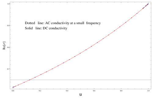
Figure 2: Flows of DC conductivity and numerical result for AC conductivity at a small frequency $\omega=0.01$. These two results matches with each other. Here we set $\lambda=0.01$, $r_{+}=1$, $\mu=0.1$ and $g=l=G_{5}=1$.

At the horizon $u_{c}=1$, the above equation becomes

$$\sigma_{\rm DC}=\frac{r_{+}}{g^{2}l},$$ (3.23)

which is consistent with (3.6). As one goes to the boundary $u_{c}\rightarrow 0$, the DC conductivity is reduced to

$$\sigma_{\rm DC}=\frac{r_{+}}{g^{2}l}\frac{(2-a)^{2}}{4(1+a)^{2}}.$$ (3.24)

which agrees with the previous result in [18]. In the absence of the chemical potential, (3.22) is reduced to the formula for DC conductivity given in [22]. However, in [22] it was assumed that the background configuration of the gauge field is not perturbed. As a matter of fact, the fluctuations of the metric and the gauge field are coupled such that the contribution of the chemical potential should not be neglected.

Next we turn to discuss the ratio of conductivity to the susceptibility. For simplicity, in the following calculation we set all the coupling parameters to be unit (i.e. $\kappa^{2}=e=g^{2}=1$) and also $l=1$. In conformal field theory, the ratio of the conductivity to the susceptibility does not depend on the relative normalization of the current and the stress tensor. Since the susceptibility is defined as

$$\chi\equiv\frac{\partial n_{q}}{\partial\mu}\bigg{|}_{T},$$ (3.25)

where $n_{q}$ is the charge density at the cut-off surface, then the expression for $\frac{\sigma_{DC}}{\chi}$ can be written as

$$\frac{\sigma_{DC}}{\chi}=\frac{1}{16\pi T}\bigg{(}\frac{2-a}{1+a}\bigg{)}^{2}=\frac{1}{4\pi T}(1-3a)+\mathcal{O}(a^{2}).$$ (3.26)

In the absence of the chemical potential $\mu=0$ (i.e. $a=0$), the above equation recovers the Einstein relation $\frac{\sigma_{DC}}{\chi}\bigg{|}_{\mu=0}=D_{c}$ with $D_{c}=\frac{1}{4\pi T}$, denoting the diffusion constant for Schwarzschild-AdS black holes [3, 18]. Since both $\sigma_{DC}$ and $\chi$ do not depend on the Gauss-Bonnet coupling, the above result implies that the Einstein relation cannot be used to derive the diffusion constant in the presence of higher-derivative gravity corrections [21]. After obtaining the conductivity, the thermal conductivity $\kappa_{T}$ can be computed using the formula [29]

$$\kappa_{T}=\bigg{(}\frac{\epsilon+P}{T_{H}n_{q}}\bigg{)}^{2}{T_{H}}\sigma_{DC}=\frac{(2-a)\pi r^{2}_{+}}{3a}.$$ (3.27)

The ratio $\frac{\kappa_{T}\mu^{2}}{\eta T_{H}}$ was computed in [29]

$$\frac{\kappa_{T}\mu^{2}}{\eta T_{H}}=\frac{2\pi^{2}}{1-2\lambda(2-a)}=2\pi^{2}\bigg{[}1+2(2-a)\lambda+4(2-a)^{2}\lambda^{2}+...\bigg{]},$$ (3.28)

where we have used (3.33). One may find that the Gauss-Bonnet coupling modify the leading behavior. Note that the leading order result given in [29] was $8\pi^{2}$ because the normalization for the gauge kinetic term differs by a factor of $4$ from that used here.

As a conjecture, we propose that the DC conductivity for single charged black branes can be evaluated through the thermal quantities (see also [28])

$$\sigma_{\rm DC}=\frac{1}{g^{2}}\sqrt{\frac{-g}{g_{uu}g_{tt}}}g^{zz}\bigg{|}_{u=1}\bigg{(}\frac{sT_{c}}{\varepsilon+p}\bigg{)}^{2}=\frac{1}{g^{2}}\sqrt{\frac{-g}{g_{uu}g_{tt}}}g^{zz}\bigg{|}_{u=1}\bigg{(}1-\frac{n_{q}\mu_{c}}{\varepsilon+p}\bigg{)}^{2},$$ (3.29)

where $s=\frac{1}{4G}u^{\frac{3}{2}}_{c}$ denotes the entropy density on the cut-off surface. Note that we have used the thermodynamical relation

$$\varepsilon+p-sT_{c}-n_{q}\mu_{c}=0.$$ (3.30)

Here the charge density and chemical potential are $n_{q}=Qu^{3/2}_{c}$ and $\mu=\frac{lQu^{1/2}_{c}}{2\sqrt{f(u_{c})}}(1-u_{c})$, respectively. One may find that (3.29) can recover the DC conductivity obtained in [17, 19] for four-dimensional RN-AdS black holes. The expression (3.29) is also consistent with [30] in the single charge case.

3.3 Diffusion constant $\bar{D}(u_{c})$ at the cutoff surface

Now we evaluate the “conductivity” introduced by the metric perturbation $a_{z}$ at zero momentum. The conductivity in this case can be defined as

$$\sigma_{h}:=\frac{j^{z}}{f_{zt}}=(-u^{2}\mathcal{M}^{\prime})\frac{j^{z}}{\tilde{f}_{zt}}.$$ (3.31)

In the zero momentum limit, the decoupled flow equation for $\sigma_{h}$ is given by

$$\frac{\partial_{u_{c}}\sigma_{h}}{-i\omega}+\frac{1}{(-u^{2}\mathcal{M}^{\prime})}\sigma^{2}_{h}\frac{g_{uu}g_{zz}}{G}-(-u^{2}\mathcal{M}^{\prime})Gg^{tt}g^{zz}=0.$$ (3.32)

Again the regularity condition at the event horizon gives

$$\sigma_{h}(u=1)=\frac{1}{16\pi G_{N}}\bigg{(}\frac{r^{3}_{+}}{l^{3}}\bigg{)}\bigg{[}1-2\lambda(2-a)\bigg{]}.$$ (3.33)

This is actually the shear viscosity for charged Gauss-Bonnet-AdS black branes because when the momentum is vanishing and thus no polarization direction, the conductivity is exactly the shear viscosity. It is worth noting that (3.33) indicates that the conductivity at the horizon obeys

$$j^{z}(1)=\sigma_{h}(1)f_{zt}(1).$$ (3.34)

This relation will be used in the following computation.

$\bullet$ Diffusion constant

In the following, we treat the vector modes in a long wave-length expansion for fields and the equations of motion. The diffusion constant will be evaluated by a line integral from the horizon to the cutoff surface. In [3], it was found that the diffusion constant runs with the variation of $u_{c}$. We will show as below that the diffusion constant not only runs with $u_{c}$, but also depends on the Gauss-Bonnet coupling constant. For non-vanishing momentum $k_{z}$, the equation of motion for $\sigma_{h}$ is coupled to other modes. To proceed further we take the scaling limit for temporal and spatial derivatives as

$$\partial_{t}\sim\epsilon^{2},~{}~{}~{}~{}\partial_{z}\sim\epsilon,$$ (3.35)

$$\tilde{f}_{zt}\sim\epsilon^{3}\bigg{(}\tilde{f}^{(0)}_{zt}+\epsilon\tilde{f}^{(1)}_{zt}+...\bigg{)},$$ (3.36)

The in-falling boundary condition at the horizon requires $j^{z}$ is linearly related to $\tilde{f}_{zt}$. Therefore, we have

$$j^{z}\sim\epsilon^{3}\bigg{(}j^{z(0)}+\epsilon j^{z(1)}+...\bigg{)}.$$ (3.37)

From the charge conservation equation, we find that

$$\tilde{j}^{t}\sim\epsilon^{2}\bigg{(}\tilde{j}^{t(0)}+\epsilon\tilde{j}^{t(1)}+...\bigg{)},$$ (3.38)

$$j^{t}\sim\epsilon^{2}\bigg{(}{j}^{t(0)}+\epsilon j^{t(1)}+...\bigg{)}.$$ (3.39)

In the lowest order, (2.24) and (2.25) reduce to

$$\partial_{u}\tilde{j}^{t(0)}=0,~{}~{}~{}\partial_{u}j^{z}=0.$$ (3.40)

The above first equation indicates that

$$\tilde{j}^{t(0)}={j}^{t(0)}-\frac{1}{g^{2}}\sqrt{-g}\frac{4u^{3}}{r^{2}_{+}}A^{\prime}_{t}A^{(0)}_{x}=C_{0},$$ (3.41)

and $C_{0}$ is a constant. The charge conservation equation (2.23) requires

$$j^{z(0)}=\tilde{j}^{t(0)}\frac{\omega}{k}.$$ (3.42)

The lowest order of the Bianchi identity becomes

$$\partial_{u}\bigg{(}\frac{\tilde{f}^{(0)}_{zt}}{-u^{2}\mathcal{M}^{\prime}}\bigg{)}=\frac{g_{uu}g_{tt}}{u\mathcal{M}G}\partial_{z}{j}^{t(0)}.$$ (3.43)

Evaluated at the horizon $u=1$, the above equation has the solution

$$\frac{\tilde{f}^{(0)}_{zt}(u)}{u^{2}\mathcal{M}^{\prime}}=\frac{\tilde{f}^{(0)}_{zt}}{u^{2}\mathcal{M}^{\prime}}\bigg{|}_{u=1}+2\kappa^{2}\int^{1}_{u}du\frac{\partial_{z}{j}^{t(0)}}{\sqrt{-g}g^{uu}g^{tt}g_{xx}u\mathcal{M}}$$ (3.44)

Using the definition of the current given in (2.17), the above equation can be written as

$$f_{zt}(u)=-\frac{\tilde{f}^{(0)}(1)}{1-2(2-a)\lambda}+2\kappa^{2}\int^{1}_{u}du\frac{\partial_{z}{j}^{t(0)}}{\sqrt{-g}g^{uu}g^{tt}g_{xx}u\mathcal{M}}.$$ (3.45)

In the scaling limit, the Maxwell equation for the gauge perturbation $A^{(0)}_{x}$ becomes

$$\partial_{u}\bigg{(}\sqrt{-g}g^{uu}g^{xx}\partial_{u}A^{(0)}_{x}\bigg{)}=\sqrt{-g}\frac{4u^{3}}{r^{2}_{+}}A^{\prime}_{t}{a}^{\prime(0)}_{t}.$$ (3.46)

Before evaluating the diffusion constant $D_{c}$ with the use of (3.45), we should first find the solution for $A^{(0)}_{x}$. Following [3], we substitute (3.46) into (3.41), further impose the boundary condition $A^{(0)}_{x}(u_{c})=0$, and then we obtain

$$A^{(0)}_{x}(u)=\frac{3a}{8\pi G[2(1+a)-3au_{c}]Q}\bigg{(}1-\frac{u}{u_{c}}\bigg{)}.$$ (3.47)

Consequently, we have

$$f_{zt}(u)=\frac{\tilde{f}^{(0)}(1)}{1-2(2-a)\lambda}+\frac{ikf(u_{c})l^{2}}{2r_{+}[2(1+a)-3au_{c}]}.$$ (3.48)

Following the sliding membrane paradigm [22], we define the conductivity by the current and electric fields as

$$\sigma_{h}(u_{c}):=\frac{j^{z(0)}(u_{c})}{f^{(0)}_{zt}(u_{c})}=\frac{\omega}{k}\frac{\tilde{j}^{t(0)}(u_{c})}{f^{(0)}_{zt}(u_{c})}.$$ (3.49)

By further using the boundary condition given in (3.34), we find the expression for the conductivity $\sigma_{h}$ from (3.48)

$$\frac{1}{\sigma_{h}(u_{c})}=\frac{1}{\sigma_{h}(1)}-\frac{k^{2}}{i\omega}\frac{{D}(u_{c})}{\sigma_{h}(1)},$$ (3.50)

where the diffusivity is

$$D(u_{c})=\frac{\frac{l^{2}}{2r_{+}}f(u_{c})}{2(1+a)-3au_{c}}\bigg{[}1-2(2-a)\lambda\bigg{]}.$$ (3.51)

The value of $D(u_{c})$ is dimensional and can be set to any value through a coordinate transformation. It is meaningful to define a dimensionless diffusion constant as what follows.

$\bullet$ Normalization of the diffusion constant

We can introduce the proper frequency $\omega_{c}$ and the proper momentum $k_{c}$ conjugate to the proper time and the proper distance respectively on the hypersurface $u=u_{c}$. We define

$$\omega_{c}\equiv\frac{\omega}{\sqrt{g_{tt}}},~{}~{}~{}~{}~{}~{}~{}k_{c}\equiv\frac{k}{\sqrt{g_{ii}}}.$$ (3.52)

The Hawking temperature at the cut-off surface $u=u_{c}$ is determined by the Tolman relation

$$T_{c}(u_{c})=\frac{T_{H}}{\sqrt{g_{tt}}},~{}~{}~{}~{}T_{H}=\frac{f^{\prime}(r_{+})}{4\pi}.$$ (3.53)

The coordinate-invariant, dimensionless diffusion constant $\bar{D}(u_{c})$ can be defined as[3]

$$\bar{D}(u_{c})=D(u_{c})T_{c}\frac{g_{zz}}{\sqrt{g_{tt}}}.$$ (3.54)

Thus the conductivity can be written in terms of the normalized momentum and the diffusion constant as follows

$$\frac{1}{\sigma_{h}(u_{c})}=\frac{1}{\sigma_{h}(1)}-\frac{k^{2}_{c}}{i\omega_{c}}\frac{\bar{D}(u_{c})/T_{c}}{\sigma_{h}(1)},$$ (3.55)

where the dimensionless diffusion constant is given by

$$\bar{D}(u_{c})=\frac{1}{4\pi N}\frac{2-a}{2(1+a)-3au_{c}}\bigg{[}1-2\lambda(2-a)\bigg{]}.$$ (3.56)

The diffusion constant obtained here depends on the charge, the position of the cut-off surface and the Gauss-Bonnet coupling. Since the conductivity and the retarded Green function has the relation

$$\sigma^{ij}(k_{\mu},u_{c})=\frac{G^{ij}_{R}(k_{\mu},u_{c})}{i\omega}.$$ (3.57)

From (3.55), we can write the related Green function $G_{z,z}$ as

$$G_{z,z}=\frac{\omega^{2}_{c}\sigma_{h}(1)}{i\omega_{c}-\bar{D}(u_{c})k^{2}/T_{c}},$$ (3.58)

where the expression for $\sigma_{h}(1)$ is given by

$$\sigma_{h}(u=1)=\frac{1}{16\pi G_{N}}\bigg{(}\frac{r^{3}_{+}}{l^{3}}\bigg{)}\bigg{[}1-2\lambda(2-a)\bigg{]}.$$ (3.59)

Our results obtained above can recover equation (4.17c) of reference [18], when $\lambda\rightarrow 0$ and $u_{c}\rightarrow 0$.

3.4 A consistent check on $\bar{D}(u_{c})$

In this section, we provide a consistent check on the diffusion constant by employing the Brown-York stress tensor $t_{ij}$ on the cut-off surface. Since the detailed computation has been presented in [31], we only summarize the main results here. The induced metric on the cutoff surface $u=u_{c}$ outside the horizon is

$$ds^{2}_{c}=\frac{r^{2}_{+}}{l^{2}}\frac{1}{u_{c}}\bigg{(}-f(u_{c})N^{2}dt^{2}+\sum^{3}_{i=1}dx^{i}dx^{i}\bigg{)}$$ (3.60)

The Brown-York stress tensor on the hypersurface with unit normal is defined by

$$t_{ij}=\frac{1}{2\kappa^{2}}\bigg{[}Kg_{ij}-K_{ij}-2\lambda(3J_{ij}-Jg_{ij})-\mathcal{C}g_{ij}\bigg{]},$$ (3.61)

with

$$J_{ij}=\frac{1}{3}\bigg{(}2KK_{ik}K^{k}_{j}+K_{kl}K^{kl}K_{ij}-2K_{ik}K^{kl}K_{lj}-K^{2}K_{ij}\bigg{)},$$ (3.62)

where $K_{ij}$ is the extrinsic curvature, $K\equiv g^{ij}K_{ij}$ and $\mathcal{C}$ is a constant. On the other hand, the stress-energy tensor of a fluid in equilibrium has its form

$$t_{ij}=(\epsilon+p)u_{i}u_{j}+pg_{ij},$$ (3.63)

with $\epsilon$ the energy density, $p$ the pressure and $u^{i}$ the normalized fluid four-velocity. It was shown in [31] that the shear viscosity from the Brown-York tensor is given by

$$\eta=\frac{1}{16\pi Gl^{3}}u^{\frac{3}{2}}_{c}\bigg{[}1-2\lambda(2-a)\bigg{]}$$ (3.64)

The sum of the energy density $\varepsilon$ and pressure $p$ is found to be [31]

$$\varepsilon+p=\frac{\bigg{[}2(1+a)u^{2}_{c}-3au^{3}_{c}\bigg{]}}{8\pi Gl\sqrt{f(u_{c})}}.$$ (3.65)

It is easy to verify that

$$\bar{D}(u_{c})=\frac{\eta}{\varepsilon+p}T_{c}=\frac{1}{4\pi N}\frac{2-a}{2(1+a)-3au_{c}}\bigg{[}1-2\lambda(2-a)\bigg{]},$$ (3.66)

which is consistent with (3.56).

4 Conclusion and discussion

In this paper, we have investigated the RG flows for transport coefficients for quark gluon plasma at finite chemical potential with charged AdS-Gauss-Bonnet black hole dual. We write down the mixed flow equations explicitly and study the corresponding conductivities. We derive an expression for the diffusion constant at a finite cutoff surface in the presence of non-vanishing chemical potential and the Gauss-Bonnet terms. The effect of turning on chemical potential can be thought of as turning on effective interaction. Actually, the mixing effect of metric and Maxwell fluctuations in charged black hole is very important because the mixing effect tells us how transverse vector modes of Maxwell fields can diffuse and longitudinal Maxwell modes can have sound modes in the presence of chemical potential.

While the diffusion constant is sensitive to the Gauss-Bonnet coupling, the computation of the DC conductivity seems to be independent of the Gauss-Bonnet coupling numerically and analytically. In addition, the structure of this paper is different from [17] since the DC conductivity is not derived from the decoupled master equations. We show that in the long wavelength limit, we only need to solve equations up to zeroth order in $\omega$.

Acknowledgments
We would like to thank the KITPC for hospitality during the course of the programm “String Phenomenology and Cosmology ” when this work is completed. The work of XHG was partly supported by NSFC, China (No. 11005072), Shanghai Rising-Star Program and Shanghai Leading Academic Discipline Project (S30105). YL was partly supported by NSFC (10875057), Fok Ying Tung Education Foundation (No.111008), the key project of Chinese Ministry of Education (No.208072), Jiangxi young scientists (JingGang Star) program and 555 talent project of Jiangxi Province. YT and XW was partly supported by NSFC (Nos. 10705048, 10731080 and 11075206) and the President Fund of GUCAS.

Appendix A Equations of motion for vector type fluctuations

We consider the shear mode in the five-dimensional RN-AdS-Gauss-Bonnet background by choosing the following gauge $a_{r}=0,~{}A_{r}=0,$ and use the Fourier decomposition

$$a_{\mu}(t,z,u)=\int\frac{d^{4}k}{(2\pi)^{4}}e^{-i\omega t+ikz}a_{\mu}(k,u),$$ (A.1)

$$A_{x}(t,z,u)=\int\frac{d^{4}k}{(2\pi)^{4}}e^{-i\omega t+ikz}A_{x}(k,u),$$ (A.2)

where we choose the momenta which are along the $z-$direction. Note that after introducing $\mathcal{M}=\frac{1-2\lambda f}{u}$, the equations of motion can be written as

$$0={a_{t}}^{\prime\prime}+\frac{\mathcal{M}^{\prime}}{\mathcal{M}}{a_{t}}^{\prime}+\frac{l^{4}b^{2}}{4f(u)}\frac{\mathcal{M}^{\prime}}{\mathcal{M}}(k^{2}a_{t}+\omega ka_{z})-\frac{3aN^{2}B^{\prime}(u)}{\mathcal{M}},$$ (A.3)

$$0=\omega{a_{t}}^{\prime}-\frac{u\mathcal{M}^{\prime}}{\mathcal{M}}f(u)N^{2}k{a_{z}}^{\prime}-\frac{3aN^{2}B(u)\omega}{\mathcal{M}},$$ (A.4)

$$0={a_{z}}^{\prime\prime}-\frac{\frac{1}{u}-\frac{f^{\prime}(u)}{f}+2\lambda[\frac{f(u)}{u}+uf^{\prime\prime}(u)+uf^{\prime}(u)^{2}/f(u)-2f^{\prime}(u)]}{1+2\lambda(uf^{\prime}(u)-f(u))}{a_{z}}^{\prime}$$

$$+\frac{l^{4}b^{2}}{4N^{2}uf^{2}(u)}(\omega ka_{t}+\omega^{2}a_{z}),$$ (A.5)

$$0=B^{\prime\prime}+\frac{f^{\prime}}{f}B^{\prime}+\frac{l^{4}b^{2}}{4N^{2}uf^{2}}(\omega^{2}-k^{2}f)B-\frac{1}{N^{2}f}{a_{t}}^{\prime},$$ (A.6)

where $b=\frac{l^{2}}{r_{+}}$, $g=1$ and the field $B$ is defined as $B=\frac{A_{x}}{\mu}=\frac{2A_{x}}{Qr_{+}}$. It is almost impossible to decouple the above equations of motion because of the mixing of the Gauss-Bonnet coupling and the charge. We leave this to the future work. For neutral black holes in Gauss-Bonnet gravity, the shear modes can be decoupled and it was analyzed in great detail by using the Kubo formula [33, 32, 34]. For tensor type perturbation for charged black holes in Gauss-Bonnet gravity, one may refer to [36, 35] (see also [37, 38, 39, 40, 41, 42]).

References

• [1] I. Heemskerk and J. Polchinski, โ€œHolographic and Wilsonian Renormalization Groups,โ€ arXiv:1010.1264 [hep-th].
• [2] T. Faulkner, H. Liu and M. Rangamani, โ€œIntegrating out geometry: Holographic Wilsonian RG and the membrane paradigm,โ€ arXiv:1010.4036 [hep-th].
• [3] I. Bredberg, C. Keeler, V. Lysov and A. Strominger, โ€œWilsonian Approach to Fluid/Gravity Duality,โ€ arXiv:1006.1902 [hep-th].
• [4] D. Nickel and D. T. Son, โ€œDeconstructing holographic liquids,โ€ New J. Phys. 13 2011 075010 [arXiv:1009.3094[hep-th]].
• [5] L. Susskind and E. Witten, โ€œThe holographic bound in anti-de Sitter space,โ€ arXiv:hep-th/9805114.
• [6] A. W. Peet and J. Polchinski, โ€œUV/IR relations in AdS dynamics,โ€ Phys. Rev. D59 (1999) 065011, arXiv:hep-th/9809022.
• [7] E. T. Akhmedov, โ€œA Remark on the AdS / CFT correspondence and the renormalization group ow,โ€ Phys.Lett. B442 (1998) 152, [arXiv:hep-th/9806217 [hep-th]].
• [8] E. Alvarez and C. Gomez, โ€œGeometric holography, the renormalization group and the c theorem,โ€ Nucl.Phys. B541 (1999) 441 [ arXiv:hep-th/9807226 [hep-th]].
• [9] L. Girardello, M. Petrini, M. Porrati, and A. Zakaroni, โ€œNovel local CFT and exact results on perturbations of N=4 superYang Mills from AdS dynamics,โ€ JHEP 9812 (1998) 022 [arXiv:hep-th/9810126 [hep-th]].
• [10] J. Distler and F. Zamora, โ€œNonsupersymmetric conformal field theories from stable anti-de Sitter spaces,โ€ Adv.Theor.Math.Phys. 2 (1999) 1405, [arXiv:hep-th/9810206 [hep-th]].
• [11] V. Balasubramanian and P. Kraus, โ€œSpace-time and the holographic renormalization group,โ€ Phys.Rev.Lett. 83 (1999) 3605 [arXiv:hep-th/9903190 [hep-th]].
• [12] D. Freedman, S. Gubser, K. Pilch, and N. Warner, โ€œRenormalization group ows from holography supersymmetry and a c theorem,โ€ Adv.Theor.Math.Phys. 3 (1999) 363 [arXiv:hep-th/9904017 [hep-th]].
• [13] J. de Boer, E. P. Verlinde, and H. L. Verlinde, โ€œOn the holographic renormalization group,โ€ JHEP 08 (2000) 003 [arXiv:hep-th/9912012].
• [14] J. de Boer,โ€œThe Holographic renormalization group,โ€ Fortsch.Phys. 49 (2001) 339, [arXiv:hep-th/0101026 [hep-th]].
• [15] M. Li, โ€œA note on relation between holographic RG equation and Polchinskiโ€™s RG equation,โ€ Nucl. Phys. B 579 (2000) 525 [arXiv:hep-th/0001193].
• [16] S. J. Sin and Y. Zhou, โ€œHolographic Wilsonian RG flow and sliding membrane paragdigm,โ€ JHEP 1105 (2011) 030 [arXiv:1102.4477[hep-th]].
• [17] Y. Matsuo, S.-J. Sin and Y. Zhou, โ€œMixed RG flows and hydrodynamics at finite holographic screen,โ€ [arXiv:1109.2698[hep-th]].
• [18] X. H. Ge, Y. Matsuo, F. W. Shu, S. J. Sin and T. Tsukioka, โ€œDensity Dependence of Transport Coefficients from Holographic Hydrodynamics,โ€ Prog. Theor. Phys. 120 (2008) 833 [arXiv:0806.4460 [hep-th]].
• [19] X. H. Ge, K. Jo and S.-J. Sin, โ€œHydrodynamics of RN AdS4 black hole and holographic optics,โ€ JHEP 1103 (2011) 104 [arXiv:1012.2515 [hep-th]].
• [20] P. Kovtun and A. Ritz, โ€œUniversal conductivity and central charges,โ€ Phys. Rev. D 78 066009 (2008) [arXiv:0806.0110[hep-th]]
• [21] R. C. Myers, M. F. Paulos and A. Sinha, โ€œHolographic hydrodynamics with a chemical potential,โ€ JHEP 0906 (2009) 006 [arXiv:0903.2834[hep-th]]
• [22] N. Iqbal and H. Liu, โ€œUniversality of the hydrodynamic limit in AdS/CFT and the membrane paradigm,โ€ Phys. Rev. D 79, 025023 (2009) [arXiv:0809.3808[hep-th]].
• [23] M. Cvetiฤ, S. Nojiri and S.D. Odintsov, Nucl. Phys. B628 (2002) 295, [arXiv:hep-th/0112045].
• [24] R. G. Cai, Phys. Rev. D 65 (2002) 084014, [arXiv:hep-th/0109133];
R.G. Cai and Q. Guo, Phys. Rev. D69 (2004) 104025, [arXiv:hep-th/0311020].
R.G. Cai, Phys. Lett. B 582 (2004) 237, [arXiv:hep-th/0311240].
• [25] I. P. Neupane, Phys. Rev. D67 (2003) 061501, [arXiv:hep-th/0212092].
• [26] D. T. Son and A. O. Starinets, โ€œMinkowski-space correlators in AdS/CFT correspondence: recipe and applications,โ€ JHEP 0209 (2002) 042 [arXiv:hep-th/0205051].
• [27] G. Policastro, D.T.Son and A.O.Starinets, โ€œFrom AdS/CFT correspondence to hydrodynamics,โ€ JHEP 0209 (2002) 043[arXiv:hep-th/0205052]
• [28] S. A. Hartnoll and C. P. Herzog, โ€œOhmโ€™s Law at strong coupling: S duality and the cyclotron resonance,โ€ Phys. Rev. D 76, 106012 (2007), [arXiv:0706.3228[hep-th]].
• [29] D. T. Son and A. O. Starinets, โ€œHydrodymacis of R-charged black holesโ€, JHEP 03 (2006) 052 [hep-th/0601157]
• [30] S. Jain, โ€œHolographic eletrical and thermal conductivity in strongly coupled gauge theory with multiple chemical potentials,โ€ [arXiv:0912.2228]
• [31] C. Niu, Y. Tian, X. N. Wu and Y. Ling, โ€œIncompressible Navier-Stokes equation from Einstein-Maxwell and Gauss-Bonnet-Maxwell theories,โ€ [arXiv:1107.1430 [hep-th]].
• [32] Y. Kats and P. Petrov, โ€œEffect of curvature squared corrections in AdS on the viscosity of the dual gauge theory,โ€ JHEP 01 (2009) 044 [arXiv:0712.0743[hep-th]].
• [33] M. Brigante, H. Liu, R.C. Myers, S. Shenker and S. Yaida, Phys. Rev. D77 (2008) 126006, [arXiv:0712.0805[hep-th]].
• [34] A. Buchel, J. Escobedo, R. C. Myers, M. F. Paulos, A. Sinhaa and M. Smolkin, โ€œHolographic GB gravity in arbitrary dimensions,โ€ [arXiv:0911.4257[hep-th]]; A. Buchel, J. Escobedo, R. C. Myers,and A. Sinha โ€œ Beyond eta/s=1/4pi,โ€ JHEP 0903, 084 (2009) [arXiv:0812.2521[hep-th]].
• [35] R. G. Cai, Z. Y. Nie and Y. W. Sun, โ€œShear Viscosity from Effective Couplings of Gravitons,โ€ arXiv:0811.1665 [hep-th];
R. G. Cai, Z. Y. Nie, N. Ohta and Y. W. Sun, โ€œShear Viscosity from Gauss-Bonnet Gravity with a Dilaton Coupling,โ€ Phys. Rev. D 79, 066004 (2009) [arXiv:0901.1421 [hep-th]].
• [36] X.ย H. Ge, Y. Matsuo, F.-W. Shu, S.-J. Sin and T. Tsukioka, โ€œViscosity Bound, Causality Violation and Instability with Stringy Correction and Charge,โ€ J. High Energy Phys. 0810, 009 (2008) [arXiv:0808.2354[hep-th]];
X.ย H. Ge and S.-J. Sin, โ€œShear viscosity, instability and the upper bound of the Gauss-Bonnet coupling constant,โ€ J. High Energy Phys. 0905, 051 (2009) [arXiv:0903.2527[hep-th]]
• [37] J. de Boer, M. Kulaxizi and A. Parnachev, [arXiv:0910.5347[hep-th]]
• [38] X. O. Camanho and J. D. Edelstein, [arXiv:0911.3160[hep-th]]; [arXiv:0912.1944[hep-th]].
• [39] Y. P. Hu, H. F. Li and Z. Y. Nie, โ€œThe first order hydrodynamics via AdS/CFT correspondence in the Gauss-Bonnet gravity,โ€ JHEP 1101 123 (2011);
Y. P. Hu, P. Sun and J. H. Zhang, โ€œHydrodynamics with conserved current via AdS/CFT correspondence in the Maxwell-Gauss-Bonnet gravity ,โ€ Phys.Rev.D 83 126003 (2011)
• [40] D. W. Pang, โ€œ On Charged Lifshitz Black Holes,โ€ JHEP 1001 (2010) 116 [arXiv:0911.2777 [hep-th] ];
D. W. Pang,โ€œR2superscript๐‘…2R^{2} Corrections to Asymptotically Lifshitz Spacetimes,โ€ JHEP 0910 031 (2009) [arXiv:0908.1272[hep-th]].
• [41] D. Astefanesei, N. Banerjee and S. Dutta, โ€œModuli and electromagnetic black brane holography,โ€ JHEP 1102 (2011) 021 [arXiv:1008.3852 [hep-th]]; D. Astefanesei, H. Nastase, H. Yavartanoo and S. Yun, โ€œ Moduli flow and non-supersymmetric AdS attractors,โ€ JHEP 0804 (2008) 074 [arXiv:0711.0036 [hep-th]].
• [42] P. Neupane and N. Dadhich, โ€œEntropy bound and causality violation in higher curvature gravity,โ€ Class. Quant. Grav. 26, (2009) 015013 [arXiv:0809.1818[hep-th]]; P. Neupane, โ€œEntropy Bound and Causality Violation,โ€ Int. J. Mod. Phys. A 24 (2009) 3584 [arXiv:0904.4805 [gr-qc]].