Information-Maximization Clustering
based on Squared-Loss Mutual Information

Abstract

Information-maximization clustering learns a probabilistic classifier in an unsupervised manner so that mutual information between feature vectors and cluster assignments is maximized. A notable advantage of this approach is that it only involves continuous optimization of model parameters, which is substantially easier to solve than discrete optimization of cluster assignments. However, existing methods still involve non-convex optimization problems, and therefore finding a good local optimal solution is not straightforward in practice. In this paper, we propose an alternative information-maximization clustering method based on a squared-loss variant of mutual information. This novel approach gives a clustering solution analytically in a computationally efficient way via kernel eigenvalue decomposition. Furthermore, we provide a practical model selection procedure that allows us to objectively optimize tuning parameters included in the kernel function. Through experiments, we demonstrate the usefulness of the proposed approach.

Keywords

Clustering, Information Maximization, Squared-Loss Mutual Information.

1 Introduction

The goal of clustering is to classify data samples into disjoint groups in an unsupervised manner. K-means (MacQueen, 1967) is a classic but still popular clustering algorithm. However, since k-means only produces linearly separated clusters, its usefulness is rather limited in practice.

To cope with this problem, various non-linear clustering methods have been developed. Kernel k-means (Girolami, 2002) performs k-means in a feature space induced by a reproducing kernel function (Schölkopf and Smola, 2002). Spectral clustering (Shi and Malik, 2000; Ng et al., 2002) first unfolds non-linear data manifolds by a spectral embedding method, and then performs k-means in the embedded space. Blurring mean-shift (Fukunaga and Hostetler, 1975; Carreira-Perpiñán, 2006) uses a non-parametric kernel density estimator for modeling the data-generating probability density, and finds clusters based on the modes of the estimated density. Discriminative clustering learns a discriminative classifier for separating clusters, where class labels are also treated as parameters to be optimized (Xu et al., 2005; Bach and Harchaoui, 2008). Dependence-maximization clustering determines cluster assignments so that their dependence on input data is maximized (Song et al., 2007; Faivishevsky and Goldberger, 2010).

These non-linear clustering techniques would be capable of handling highly complex real-world data. However, they suffer from lack of objective model selection strategies. More specifically, the above non-linear clustering methods contain tuning parameters such as the width of Gaussian functions and the number of nearest neighbors in kernel functions or similarity measures, and these tuning parameter values need to be manually determined in an unsupervised manner. The problem of learning similarities/kernels was addressed in earlier works (Meila and Shi, 2001; Shental et al., 2003; Cour et al., 2005; Bach and Jordan, 2006), but they considered supervised setups, i.e., labeled samples are assumed to be given. Zelnik-Manor and Perona (2005) provided a useful unsupervised heuristic to determine the similarity in a data-dependent way. However, it still requires the number of nearest neighbors to be determined manually (although the magic number ‘7’ was shown to work well in their experiments).

Another line of clustering framework called information-maximization clustering exhibited the state-of-the-art performance (Agakov and Barber, 2006; Gomes et al., 2010). In this information-maximization approach, probabilistic classifiers such as a kernelized Gaussian classifier (Agakov and Barber, 2006) and a kernel logistic regression classifier (Gomes et al., 2010) are learned so that mutual information (MI) between feature vectors and cluster assignments is maximized in an unsupervised manner. A notable advantage of this approach is that classifier training is formulated as continuous optimization problems, which are substantially simpler than discrete optimization of cluster assignments. Indeed, classifier training can be carried out in computationally efficient manners by a gradient method (Agakov and Barber, 2006) or a quasi-Newton method (Gomes et al., 2010). Furthermore, Agakov and Barber (2006) provided a model selection strategy based on the information-maximization principle. Thus, kernel parameters can be systematically optimized in an unsupervised way.

However, in the above MI-based clustering approach, the optimization problems are non-convex, and finding a good local optimal solution is not straightforward in practice. The goal of this paper is to overcome this problem by providing a novel information-maximization clustering method. More specifically, we propose to employ a variant of MI called squared-loss MI (SMI), and develop a new clustering algorithm whose solution can be computed analytically in a computationally efficient way via kernel eigenvalue decomposition. Furthermore, for kernel parameter optimization, we propose to use a non-parametric SMI estimator called least-squares MI (LSMI; Suzuki et al., 2009), which was proved to achieve the optimal convergence rate with analytic-form solutions. Through experiments on various real-world datasets such as images, natural languages, accelerometric sensors, and speech, we demonstrate the usefulness of the proposed clustering method.

The rest of this paper is structured as follows. In Section 2, we describe our proposed information-maximization clustering method based on SMI. Then the proposed method is compared with existing clustering methods qualitatively in Section 3 and quantitatively in Section 4. Finally, this paper is concluded in Section 5.

2 Information-Maximization Clustering with Squared-Loss Mutual Information

In this section, we describe our proposed clustering algorithm.

2.1 Formulation of Information-Maximization Clustering

Suppose we are given $d$-dimensional i.i.d. feature vectors of size $n$,

$$\{{\bm{x}}_{i}\;|\;{\bm{x}}_{i}\in\mathbb{R}^{d}\}_{i=1}^{n},$$

which are assumed to be drawn independently from a distribution with density $p^{\ast}({\bm{x}})$. The goal of clustering is to give cluster assignments,

$$\{y_{i}\;|\;y_{i}\in\{1,\ldots,c\}\}_{i=1}^{n},$$

to the feature vectors $\{{\bm{x}}_{i}\}_{i=1}^{n}$, where $c$ denotes the number of classes. Throughout this paper, we assume that $c$ is known.

In order to solve the clustering problem, we take the information-maximization approach (Agakov and Barber, 2006; Gomes et al., 2010). That is, we regard clustering as an unsupervised classification problem, and learn the class-posterior probability $p^{\ast}(y|{\bm{x}})$ so that ‘information’ between feature vector ${\bm{x}}$ and class label $y$ is maximized.

The dependence-maximization approach (Song et al., 2007; Faivishevsky and Goldberger, 2010, see also Section 3.7) is related to, but substantially different from the above information-maximization approach. In the dependence-maximization approach, cluster assignments $\{y_{i}\}_{i=1}^{n}$ are directly determined so that their dependence on feature vectors $\{{\bm{x}}_{i}\}_{i=1}^{n}$ is maximized. Thus, the dependence-maximization approach intrinsically involves combinatorial optimization with respect to $\{y_{i}\}_{i=1}^{n}$. On the other hand, the information-maximization approach involves continuous optimization with respect to the parameter ${\bm{\alpha}}$ included in a class-posterior model $p(y|{\bm{x}};{\bm{\alpha}})$. This continuous optimization of ${\bm{\alpha}}$ is substantially easier to solve than discrete optimization of $\{y_{i}\}_{i=1}^{n}$.

Another advantage of the information-maximization approach is that it naturally allows out-of-sample clustering based on the discriminative model $p(y|{\bm{x}};{\bm{\alpha}})$, i.e., a cluster assignment for a new feature vector can be obtained based on the learned discriminative model.

2.2 Squared-Loss Mutual Information

As an information measure, we adopt squared-loss mutual information (SMI). SMI between feature vector ${\bm{x}}$ and class label $y$ is defined by

$$\mathrm{SMI} :=\frac{1}{2}\int\sum_{y=1}^{c}p^{\ast}({\bm{x}})p^{\ast}(y)\left(\frac{p^{\ast}({\bm{x}},y)}{p^{\ast}({\bm{x}})p^{\ast}(y)}-1\right)^{2}\mathrm{d}{\bm{x}},$$ (1)

where $p^{\ast}({\bm{x}},y)$ denotes the joint density of ${\bm{x}}$ and $y$, and $p^{\ast}(y)$ is the marginal probability of $y$. SMI is the Pearson divergence (Pearson, 1900) from $p^{\ast}({\bm{x}},y)$ to $p^{\ast}({\bm{x}})p^{\ast}(y)$, while the ordinary MI (Cover and Thomas, 2006),

$$\mathrm{MI}:=\int\sum_{y=1}^{c}p^{\ast}({\bm{x}},y)\log\frac{p^{\ast}({\bm{x}},y)}{p^{\ast}({\bm{x}})p^{\ast}(y)}\mathrm{d}{\bm{x}},$$ (2)

is the Kullback-Leibler divergence (Kullback and Leibler, 1951) from $p^{\ast}({\bm{x}},y)$ to $p^{\ast}({\bm{x}})p^{\ast}(y)$. The Pearson divergence and the Kullback-Leibler divergence both belong to the class of Ali-Silvey-Csiszár divergences (which is also known as $f$-divergences, see Ali and Silvey, 1966; Csiszár, 1967), and thus they share similar properties. For example, SMI is non-negative and takes zero if and only if ${\bm{x}}$ and $y$ are statistically independent, as the ordinary MI.

In the existing information-maximization clustering methods (Agakov and Barber, 2006; Gomes et al., 2010, see also Section 3.8), MI is used as the information measure. On the other hand, in this paper, we adopt SMI because it allows us to develop a clustering algorithm whose solution can be computed analytically in a computationally efficient way via kernel eigenvalue decomposition.

2.3 Clustering by SMI Maximization

Here, we give a computationally-efficient clustering algorithm based on SMI (1).

Expanding the squared term in Eq.(1), we can express SMI as

$$\mathrm{SMI} =\frac{1}{2}\int\sum_{y=1}^{c}p^{\ast}({\bm{x}})p^{\ast}(y)\left(\frac{p^{\ast}({\bm{x}},y)}{p^{\ast}({\bm{x}})p^{\ast}(y)}\right)^{2}\mathrm{d}{\bm{x}}$$

$$\phantom{=}-\int\sum_{y=1}^{c}p^{\ast}({\bm{x}})p^{\ast}(y)\frac{p^{\ast}({\bm{x}},y)}{p^{\ast}({\bm{x}})p^{\ast}(y)}\mathrm{d}{\bm{x}}+\frac{1}{2}$$

$$=\frac{1}{2}\int\sum_{y=1}^{c}p^{\ast}(y|{\bm{x}})p^{\ast}({\bm{x}})\frac{p^{\ast}(y|{\bm{x}})}{p^{\ast}(y)}\mathrm{d}{\bm{x}}-\frac{1}{2}.$$ (3)

Suppose that the class-prior probability $p^{\ast}(y)$ is set to a user-specified value $\pi_{y}$ for $y=1,\ldots,c$, where $\pi_{y}>0$ and $\sum_{y=1}^{c}\pi_{y}=1$. Without loss of generality, we assume that $\{\pi_{y}\}_{y=1}^{c}$ are sorted in the ascending order:

$$\pi_{1}\leq\cdots\leq\pi_{c}.$$

If $\{\pi_{y}\}_{y=1}^{c}$ is unknown, we may merely adopt the uniform class-prior distribution:

$$p^{\ast}(y)=\frac{1}{c}\mbox{ for }y=1,\ldots,c,$$ (4)

which will be non-informative and thus allow us to avoid biasing clustering solutions. Substituting $\pi_{y}$ into $p^{\ast}(y)$, we can express Eq.(3) as

$$\frac{1}{2}\int\sum_{y=1}^{c}\frac{1}{\pi_{y}}p^{\ast}(y|{\bm{x}})p^{\ast}({\bm{x}})p^{\ast}(y|{\bm{x}})\mathrm{d}{\bm{x}}-\frac{1}{2}.$$ (5)

Let us approximate the class-posterior probability $p^{\ast}(y|{\bm{x}})$ by the following kernel model:

$$p(y|{\bm{x}};{\bm{\alpha}}) :=\sum_{i=1}^{n}\alpha_{y,i}K({\bm{x}},{\bm{x}}_{i}),$$ (6)

where ${\bm{\alpha}}=(\alpha_{1,1},\ldots,\alpha_{c,n})^{\top}$ is the parameter vector, ^⊤ denotes the transpose, and $K({\bm{x}},{\bm{x}}^{\prime})$ denotes a kernel function with a kernel parameter $t$. In the experiments, we will use a sparse variant of the local-scaling kernel (Zelnik-Manor and Perona, 2005):

$$K({\bm{x}}_{i},{\bm{x}}_{j})=\begin{cases}\displaystyle\exp\left(-\frac{\|{\bm{x}}_{i}-{\bm{x}}_{j}\|^{2}}{2\sigma_{i}\sigma_{j}}\right)&\mbox{if ${\bm{x}}_{i}\in{\mathcal{N}}_{t}({\bm{x}}_{j})$ or ${\bm{x}}_{j}\in{\mathcal{N}}_{t}({\bm{x}}_{i})$},\\[14.22636pt] 0&\mbox{otherwise},\end{cases}$$ (7)

where ${\mathcal{N}}_{t}({\bm{x}})$ denotes the set of $t$ nearest neighbors for ${\bm{x}}$ ($t$ is the kernel parameter), $\sigma_{i}$ is a local scaling factor defined as $\sigma_{i}=\|{\bm{x}}_{i}-{\bm{x}}_{i}^{(t)}\|$, and ${\bm{x}}_{i}^{(t)}$ is the $t$-th nearest neighbor of ${\bm{x}}_{i}$.

Further approximating the expectation with respect to $p^{\ast}({\bm{x}})$ included in Eq.(5) by the empirical average of samples $\{{\bm{x}}_{i}\}_{i=1}^{n}$, we arrive at the following SMI approximator:

$$\widehat{\mathrm{SMI}} :=\frac{1}{2n}\sum_{y=1}^{c}\frac{1}{\pi_{y}}{\bm{\alpha}}_{y}^{\top}{\bm{K}}^{2}{\bm{\alpha}}_{y}-\frac{1}{2},$$ (8)

where ${\bm{\alpha}}_{y}:=(\alpha_{y,1},\ldots,\alpha_{y,n})^{\top}$ and $K_{i,j}:=K({\bm{x}}_{i},{\bm{x}}_{j})$.

For each cluster $y$, we maximize ${\bm{\alpha}}_{y}^{\top}{\bm{K}}^{2}{\bm{\alpha}}_{y}$ under $\|{\bm{\alpha}}_{y}\|=1$. Since this is the Rayleigh quotient, the maximizer is given by the normalized principal eigenvector of ${\bm{K}}$ (Horn and Johnson, 1985). To avoid all the solutions $\{{\bm{\alpha}}_{y}\}_{y=1}^{c}$ to be reduced to the same principal eigenvector, we impose their mutual orthogonality: ${\bm{\alpha}}_{y}^{\top}{\bm{\alpha}}_{y^{\prime}}=0$ for $y\neq y^{\prime}$. Then the solutions are given by the normalized eigenvectors ${\bm{\phi}}_{1},\ldots,{\bm{\phi}}_{c}$ associated with the eigenvalues $\lambda_{1}\geq\cdots\geq\lambda_{n}\geq 0$ of ${\bm{K}}$. Since the sign of ${\bm{\phi}}_{y}$ is arbitrary, we set the sign as

$$\widetilde{{\bm{\phi}}}_{y}={\bm{\phi}}_{y}\times\mathrm{sign}({\bm{\phi}}_{y}^{\top}{\bm{1}}_{n}),$$

where $\mathrm{sign}(\cdot)$ denotes the sign of a scalar and ${\bm{1}}_{n}$ denotes the $n$-dimensional vector with all ones.

On the other hand, since

$$p^{\ast}(y)=\int p^{\ast}(y|{\bm{x}})p^{\ast}({\bm{x}})\mathrm{d}{\bm{x}}\approx\frac{1}{n}\sum_{i=1}^{n}p(y|{\bm{x}}_{i};{\bm{\alpha}})={\bm{\alpha}}_{y}^{\top}{\bm{K}}{\bm{1}}_{n},$$

and the class-prior probability $p^{\ast}(y)$ was set to $\pi_{y}$ for $y=1,\ldots,c$, we have the following normalization condition:

$${\bm{\alpha}}_{y}^{\top}{\bm{K}}{\bm{1}}_{n}=\pi_{y}.$$

Furthermore, probability estimates should be non-negative, which can be achieved by rounding up negative outputs to zero.

Taking these normalization and non-negativity issues into account, cluster assignment $y_{i}$ for ${\bm{x}}_{i}$ is determined as the maximizer of the approximation of $p(y|{\bm{x}}_{i})$:

$$y_{i} =\mathop{\mathrm{argmax\,}}_{y}\frac{[\max({\bm{0}}_{n},{\bm{K}}\widetilde{{\bm{\phi}}}_{y})]_{i}}{\pi_{y}^{-1}\max({\bm{0}}_{n},{\bm{K}}\widetilde{{\bm{\phi}}}_{y})^{\top}{\bm{1}}_{n}}=\mathop{\mathrm{argmax\,}}_{y}\frac{\pi_{y}[\max({\bm{0}}_{n},\widetilde{{\bm{\phi}}}_{y})]_{i}}{\max({\bm{0}}_{n},\widetilde{{\bm{\phi}}}_{y})^{\top}{\bm{1}}_{n}},$$

where the max operation for vectors is applied in the element-wise manner and $[\cdot]_{i}$ denotes the $i$-th element of a vector. Note that we used ${\bm{K}}\widetilde{{\bm{\phi}}}_{y}=\lambda_{y}\widetilde{{\bm{\phi}}}_{y}$ in the above derivation. For out-of-sample prediction, cluster assignment $y^{\prime}$ for new sample ${\bm{x}}^{\prime}$ may be obtained as

$$y^{\prime} :=\mathop{\mathrm{argmax\,}}_{y}\frac{\pi_{y}\max\left(0,\sum_{i=1}^{n}K({\bm{x}}^{\prime},{\bm{x}}_{i})[\widetilde{{\bm{\phi}}}_{y}]_{i}\right)}{\lambda_{y}\max({\bm{0}}_{n},\widetilde{{\bm{\phi}}}_{y})^{\top}{\bm{1}}_{n}}.$$

We call the above method SMI-based clustering (SMIC).

2.4 Kernel Parameter Choice by SMI Maximization

The solution of SMIC depends on the choice of the kernel parameter $t$ included in the kernel function $K({\bm{x}},{\bm{x}}^{\prime})$. Since SMIC was developed in the framework of SMI maximization, it would be natural to determine the kernel parameter $t$ so as to maximize SMI. A direct approach is to use the SMI estimator $\widehat{\mathrm{SMI}}$ (8) also for kernel parameter choice. However, this direct approach is not favorable because $\widehat{\mathrm{SMI}}$ is an unsupervised SMI estimator (i.e., SMI is estimated only from unlabeled samples $\{{\bm{x}}_{i}\}_{i=1}^{n}$). On the other hand, in the model selection stage, we have already obtained labeled samples $\{({\bm{x}}_{i},y_{i})\}_{i=1}^{n}$, and thus supervised estimation of SMI is possible. For supervised SMI estimation, a non-parametric SMI estimator called least-squares mutual information (LSMI; Suzuki et al., 2009) was shown to achieve the optimal convergence rate. For this reason, we propose to use LSMI for model selection, instead of $\widehat{\mathrm{SMI}}$ (8).

LSMI is an estimator of SMI based on paired samples $\{({\bm{x}}_{i},y_{i})\}_{i=1}^{n}$. The key idea of LSMI is to learn the following density-ratio function,

$$r^{\ast}({\bm{x}},y):=\frac{p^{\ast}({\bm{x}},y)}{p^{\ast}({\bm{x}})p^{\ast}(y)},$$ (9)

without going through density estimation of $p^{\ast}({\bm{x}},y)$, $p^{\ast}({\bm{x}})$, and $p^{\ast}(y)$. More specifically, let us employ the following density-ratio model:

$$r({\bm{x}},y;{\bm{\theta}}) :=\sum_{\ell:y_{\ell}=y}\theta_{\ell}L({\bm{x}},{\bm{x}}_{\ell}),$$ (10)

where ${\bm{\theta}}=(\theta_{1},\ldots,\theta_{n})^{\top}$ and $L({\bm{x}},{\bm{x}}^{\prime})$ is a kernel function with a kernel parameter $\gamma$. In the experiments, we will use the Gaussian kernel:

$$L({\bm{x}},{\bm{x}}^{\prime})=\exp\left(-\frac{\|{\bm{x}}-{\bm{x}}^{\prime}\|^{2}}{2\gamma^{2}}\right),$$ (11)

where the Gaussian width $\gamma$ is the kernel parameter.

The parameter ${\bm{\theta}}$ in the above density-ratio model is learned so that the following squared error is minimized:

$$\min_{\bm{\theta}}\frac{1}{2}\int\sum_{y=1}^{c}\Big{(}r({\bm{x}},y;{\bm{\theta}})-r^{\ast}({\bm{x}},y)\Big{)}^{2}p^{\ast}({\bm{x}})p^{\ast}(y)\mathrm{d}{\bm{x}}.$$ (12)

Let ${\bm{\theta}}_{y}$ be the parameter vector corresponding to the kernel bases $\{L({\bm{x}},{\bm{x}}_{\ell})\}_{\ell:y_{\ell}=y}$, i.e., ${\bm{\theta}}_{y}$ is the sub-vector of ${\bm{\theta}}=(\theta_{1},\ldots,\theta_{n})^{\top}$ consisting of indices $\{\ell\;|\;y_{\ell}=y\}$. Let $n_{y}$ be the length of ${\bm{\theta}}_{y}$, i.e., the number of samples in cluster $y$. Then an empirical and regularized version of the optimization problem (12) is given for each $y$ as follows:

$$\min_{{\bm{\theta}}_{y}}\left[\frac{1}{2}{\bm{\theta}}_{y}^{\top}{\widehat{{\bm{H}}}}^{(y)}{\bm{\theta}}_{y}-{\bm{\theta}}_{y}^{\top}{\widehat{{\bm{h}}}}^{(y)}+\frac{\delta}{2}{\bm{\theta}}_{y}^{\top}{\bm{\theta}}_{y}\right],$$ (13)

where $\delta$ ($\geq 0$) is the regularization parameter. ${\widehat{{\bm{H}}}}^{(y)}$ is the $n_{y}\times n_{y}$ matrix and ${\widehat{{\bm{h}}}}^{(y)}$ is the $n_{y}$-dimensional vector defined as

$${\widehat{H}}_{\ell,\ell^{\prime}}^{(y)} :=\frac{n_{y}}{n^{2}}\sum_{i=1}^{n}L({\bm{x}}_{i},{\bm{x}}_{\ell}^{(y)})L({\bm{x}}_{i},{\bm{x}}_{\ell^{\prime}}^{(y)}),$$

$${\widehat{h}}_{\ell}^{(y)} :=\frac{1}{n}\sum_{i:y_{i}=y}L({\bm{x}}_{i},{\bm{x}}_{\ell}^{(y)}),$$

where ${\bm{x}}^{(y)}_{\ell}$ is the $\ell$-th sample in class $y$ (which corresponds to ${\widehat{\theta}}^{(y)}_{\ell}$).

A notable advantage of LSMI is that the solution ${\widehat{{\bm{\theta}}}}^{(y)}$ can be computed analytically as

$${\widehat{{\bm{\theta}}}}^{(y)}=({\widehat{{\bm{H}}}}^{(y)}+\delta{\bm{I}})^{-1}{\widehat{{\bm{h}}}}^{(y)}.$$

Then a density-ratio estimator is obtained analytically as follows:

$$\widehat{r}({\bm{x}},y) =\sum_{\ell=1}^{n_{y}}{\widehat{\theta}}^{(y)}_{\ell}L({\bm{x}},{\bm{x}}^{(y)}_{\ell}).$$

The accuracy of the above least-squares density-ratio estimator depends on the choice of the kernel parameter $\gamma$ included in $L({\bm{x}},{\bm{x}}^{\prime})$ and the regularization parameter $\delta$ in Eq.(13). Suzuki et al. (2009) showed that these tuning parameter values can be systematically optimized based on cross-validation as follows: First, the samples ${\mathcal{Z}}=\{({\bm{x}}_{i},y_{i})\}_{i=1}^{n}$ are divided into $M$ disjoint subsets $\{{\mathcal{Z}}_{m}\}_{m=1}^{M}$ of approximately the same size (we use $M=5$ in the experiments). Then a density-ratio estimator $\widehat{r}_{m}({\bm{x}},y)$ is obtained using ${\mathcal{Z}}\backslash{\mathcal{Z}}_{m}$ (i.e., all samples without ${\mathcal{Z}}_{m}$), and its out-of-sample error (which corresponds to Eq.(12) without irrelevant constant) for the hold-out samples ${\mathcal{Z}}_{m}$ is computed as

$$\mathrm{CV}_{m}:=\frac{1}{2|{\mathcal{Z}}_{m}|^{2}}\sum_{{\bm{x}},y\in{\mathcal{Z}}_{m}}\widehat{r}_{m}({\bm{x}},y)^{2}-\frac{1}{|{\mathcal{Z}}_{m}|}\sum_{({\bm{x}},y)\in{\mathcal{Z}}_{m}}\widehat{r}_{m}({\bm{x}},y).$$

This procedure is repeated for $m=1,\ldots,M$, and the average of the above hold-out error over all $m$ is computed as

$$\mathrm{CV}:=\frac{1}{M}\sum_{m=1}^{M}\mathrm{CV}_{m}.$$

Finally, the kernel parameter $\gamma$ and the regularization parameter $\delta$ that minimize the average hold-out error $\mathrm{CV}$ are chosen as the most suitable ones.

Finally, based on an expression of SMI (1),

$$\mathrm{SMI} =-\frac{1}{2}\int\sum_{y=1}^{c}r^{\ast}({\bm{x}},y)^{2}p^{\ast}({\bm{x}})p^{\ast}(y)\mathrm{d}{\bm{x}}+\int\sum_{y=1}^{c}r^{\ast}({\bm{x}},y)p^{\ast}({\bm{x}},y)\mathrm{d}{\bm{x}}-\frac{1}{2},$$

an SMI estimator called LSMI is given as follows:

$$\mathrm{LSMI}:=-\frac{1}{2n^{2}}\sum_{i,j=1}^{n}\widehat{r}({\bm{x}}_{i},y_{j})^{2}+\frac{1}{n}\sum_{i=1}^{n}\widehat{r}({\bm{x}}_{i},y_{i})-\frac{1}{2},$$ (14)

where $\widehat{r}({\bm{x}},y)$ is a density-ratio estimator obtained above. Since $\widehat{r}({\bm{x}},y)$ can be computed analytically, LSMI can also be computed analytically.

We use LSMI for model selection of SMIC. More specifically, we compute LSMI as a function of the kernel parameter $t$ of $K({\bm{x}},{\bm{x}}^{\prime})$ included in the cluster-posterior model (6), and choose the one that maximizes LSMI. A pseudo code of the entire SMI-maximization clustering procedure is summarized in Figures 1–3. Its MATLAB implementation is available from

‘http://sugiyama-www.cs.titech.ac.jp/~sugi/software/SMIC’.

Input: Feature vectors ${\mathcal{X}}=\{{\bm{x}}_{i}\}_{i=1}^{n}$ and the number $c$ of clusters Output: Cluster assignments ${\mathcal{Y}}=\{y_{i}\}_{i=1}^{n}$ For each kernel parameter candidate $t\in T$ ${\mathcal{Y}}^{(t)}\longleftarrow\mathrm{SMIC}({\mathcal{X}},t,c)$; $\mathrm{LSMI}(t)\longleftarrow\mathrm{LSMI}({\mathcal{X}},{\mathcal{Y}}^{(t)})$; end $\displaystyle\widehat{t}\longleftarrow\mathop{\mathrm{argmax\,}}_{t\in T}\mathrm{LSMI}(t)$; ${\mathcal{Y}}\longleftarrow{\mathcal{Y}}^{(\widehat{t})}$;

Figure 1: Pseudo code of information-maximization clustering based on SMIC and LSMI. The kernel parameter $t$ refers to the tuning parameter included in the kernel function $K({\bm{x}},{\bm{x}}^{\prime})$ in the cluster-posterior model (6). Pseudo codes of SMIC and LSMI are described in Figure 3 and Figure 3, respectively.

Input: Feature vectors ${\mathcal{X}}=\{{\bm{x}}_{i}\}_{i=1}^{n}$, kernel parameter $t$,   Input: and the number $c$ of clusters Output: Cluster assignments ${\mathcal{Y}}=\{y_{i}\}_{i=1}^{n}$ ${\bm{K}}\longleftarrow$ Kernel matrix for samples ${\mathcal{X}}$ and kernel parameter $t$; ${\bm{\phi}}_{y}\longleftarrow$ $y$-th principal eigenvectors of ${\bm{K}}$ for $y=1,\ldots,c$; $\widetilde{{\bm{\phi}}}_{y}\longleftarrow{\bm{\phi}}_{y}\times\mathrm{sign}({\bm{\phi}}_{y}^{\top}{\bm{1}}_{n})$ for $y=1,\ldots,c$; $\displaystyle y_{i}\longleftarrow\mathop{\mathrm{argmax\,}}_{y\in\{1,\ldots,c\}}\frac{[\max({\bm{0}}_{n},\widetilde{{\bm{\phi}}}_{y})]_{i}}{\max({\bm{0}}_{n},\widetilde{{\bm{\phi}}}_{y})^{\top}{\bm{1}}_{n}}$ for $i=1,\ldots,n$; ${\mathcal{Y}}\longleftarrow\{y_{i}\}_{i=1}^{n}$; Input: Feature vectors ${\mathcal{X}}=\{{\bm{x}}_{i}\}_{i=1}^{n}$ and cluster assignments ${\mathcal{Y}}=\{y_{i}\}_{i=1}^{n}$ Output: SMI estimate $\mathrm{LSMI}$ ${\mathcal{Z}}\longleftarrow\{({\bm{x}}_{i},y_{i})\}_{i=1}^{n}$; $\{{\mathcal{Z}}_{m}\}_{m=1}^{M}\longleftarrow$ $M$ disjoint subsets of ${\mathcal{Z}}$; For each kernel parameter candidate $\gamma\in\Gamma$ For each regularization parameter candidate $\delta\in\Delta$ For each fold $m=1,\ldots,M$ $\widehat{r}_{\gamma,\delta,m}({\bm{x}},y)\longleftarrow$ Density ratio estimator for $(\gamma,\delta)$ using ${\mathcal{Z}}\backslash{\mathcal{Z}}_{m}$; $\mathrm{CV}_{m}(\gamma,\delta)\longleftarrow$ Hold-out error of $\widehat{r}_{\gamma,\delta,m}({\bm{x}},y)$ for ${\mathcal{Z}}_{m}$; end $\displaystyle\mathrm{CV}(\gamma,\delta)\longleftarrow\frac{1}{M}\sum_{m=1}^{M}\mathrm{CV}_{m}(\gamma,\delta)$; end end $\displaystyle(\widehat{\gamma},\widehat{\delta})\longleftarrow\mathop{\mathrm{argmin\,}}_{\gamma\in\Gamma,\delta\in\Delta}\mathrm{CV}(\gamma,\delta)$; $\widehat{r}({\bm{x}},y)\longleftarrow$ Density ratio estimator for $(\widehat{\gamma},\widehat{\delta})$ using ${\mathcal{Z}}$; $\displaystyle\mathrm{LSMI}\longleftarrow-\frac{1}{2n^{2}}\sum_{i,j=1}^{n}\widehat{r}({\bm{x}}_{i},y_{j})^{2}+\frac{1}{n}\sum_{i=1}^{n}\widehat{r}({\bm{x}}_{i},y_{i})-\frac{1}{2},$;

Figure 2: Pseudo code of SMIC (with the uniform class-prior distribution). The kernel parameter $t$ refers to the tuning parameter included in the kernel function $K({\bm{x}},{\bm{x}}^{\prime})$ in the cluster-posterior model (6). If the class-prior probability $p^{\ast}(y)$ is set to a user-specified value $\pi_{y}$ for $y=1,\ldots,c$, $y_{i}$ is determined as $\mathop{\mathrm{argmax\,}}_{y}\frac{\pi_{y}[\max({\bm{0}}_{n},\widetilde{{\bm{\phi}}}_{y})]_{i}}{\max({\bm{0}}_{n},\widetilde{{\bm{\phi}}}_{y})^{\top}{\bm{1}}_{n}}$.

Figure 3: Pseudo code of LSMI. The kernel parameter $\gamma$ refers to the tuning parameter included in the kernel function $L({\bm{x}},{\bm{x}}^{\prime})$ in the density-ratio model (10).

3 Existing Clustering Methods

In this section, we review existing clustering methods and qualitatively discuss the relation to the proposed approach.

3.1 K-Means Clustering

K-means clustering (MacQueen, 1967) would be one of the most popular clustering algorithms. It tries to minimize the following distortion measure with respect to the cluster assignments $\{y_{i}\}_{i=1}^{n}$:

$$\sum_{y=1}^{c}\sum_{i:y_{i}=y}\|{\bm{x}}_{i}-{\bm{\mu}}_{y}\|^{2},$$ (15)

where ${\bm{\mu}}_{y}:=\frac{1}{n_{y}}\sum_{i:y_{i}=y}{\bm{x}}_{i}$ is the centroid of cluster $y$ and $n_{y}$ is the number of samples in cluster $y$.

The original k-means algorithm is capable of only producing linearly separated clusters (Duda et al., 2001). However, since samples are used only in terms of their inner products, its non-linear variant can be immediately obtained by performing k-means in a feature space induced by a reproducing kernel function (Girolami, 2002).

As the optimization problem of (kernel) k-means is NP-hard (Aloise et al., 2009), a greedy optimization algorithm is usually used for finding a local optimal solution in practice. It was shown that the solution to a continuously-relaxed variant of the kernel k-means problem is given by the principal components of the kernel matrix (Zha et al., 2002; Ding and He, 2004). Thus, post-discretization of the relaxed solution may give a good approximation to the original problem, which is computationally efficient. This idea is similar to the proposed SMIC method described in Section 2.3. However, an essential difference is that SMIC handles the continuous solution directly as a parameter estimate of the class-posterior model.

The performance of kernel k-means depends heavily on the choice of kernel functions, and there is no systematic way to determine the kernel function. This is a critical weakness of kernel k-means in practice. On the other hand, our proposed approach offers a natural model selection strategy, which is a significant advantage over kernel k-means.

3.2 Spectral Clustering

The basic idea of spectral clustering (Shi and Malik, 2000; Ng et al., 2002) is to first unfold non-linear data manifolds by a spectral embedding method, and then perform k-means in the embedded space. More specifically, given sample-sample similarity $W_{i,j}\geq 0$ (large $W_{i,j}$ means that ${\bm{x}}_{i}$ and ${\bm{x}}_{j}$ are similar), the minimizer of the following criterion with respect to $\{{\bm{\xi}}_{i}\}_{i=1}^{n}$ is obtained under some normalization constraint:

$$\sum_{i,j}^{n}W_{i,j}\left\|\frac{1}{\sqrt{D_{i,i}}}{\bm{\xi}}_{i}-\frac{1}{\sqrt{D_{j,j}}}{\bm{\xi}}_{j}\right\|^{2},$$

where ${\bm{D}}$ is the diagonal matrix with $i$-th diagonal element given by $D_{i,i}:=\sum_{j=1}^{n}W_{i,j}$. Consequently, the embedded samples are given by the principal eigenvectors of ${\bm{D}}^{-\frac{1}{2}}{\bm{W}}{\bm{D}}^{-\frac{1}{2}}$, followed by normalization. Note that spectral clustering was shown to be equivalent to a weighted variant of kernel k-means with some specific kernel (Dhillon et al., 2004).

The performance of spectral clustering depends heavily on the choice of sample-sample similarity $W_{i,j}$. Zelnik-Manor and Perona (2005) proposed a useful unsupervised heuristic to determine the similarity in a data-dependent manner, called local scaling:

$$W_{i,j}=\exp\left(-\frac{\|{\bm{x}}_{i}-{\bm{x}}_{j}\|^{2}}{2\sigma_{i}\sigma_{j}}\right),$$

where $\sigma_{i}$ is a local scaling factor defined as

$$\sigma_{i}=\|{\bm{x}}_{i}-{\bm{x}}_{i}^{(t)}\|,$$

and ${\bm{x}}_{i}^{(t)}$ is the $t$-th nearest neighbor of ${\bm{x}}_{i}$. $t$ is the tuning parameter in the local scaling similarity, and $t=7$ was shown to be useful (Zelnik-Manor and Perona, 2005; Sugiyama, 2007). However, this magic number ‘7’ does not seem to work always well in general.

If ${\bm{D}}^{-\frac{1}{2}}{\bm{W}}{\bm{D}}^{-\frac{1}{2}}$ is regarded as a kernel matrix, spectral clustering will be similar to the proposed SMIC method described in Section 2.3. However, SMIC does not require the post k-means processing since the principal components have clear interpretation as parameter estimates of the class-posterior model (6). Furthermore, our proposed approach provides a systematic model selection strategy, which is a notable advantage over spectral clustering.

3.3 Blurring Mean-Shift Clustering

Blurring mean-shift (Fukunaga and Hostetler, 1975) is a non-parametric clustering method based on the modes of the data-generating probability density.

In the blurring mean-shift algorithm, a kernel density estimator (Silverman, 1986) is used for modeling the data-generating probability density:

$$\widehat{p}({\bm{x}})=\frac{1}{n}\sum_{i=1}^{n}K\left({\left\|{\bm{x}}-{\bm{x}}_{i}\right\|^{2}}/{\sigma^{2}}\right),$$

where $K(\xi)$ is a kernel function such as a Gaussian kernel $K(\xi)=e^{-\xi/2}$. Taking the derivative of $\widehat{p}({\bm{x}})$ with respect to ${\bm{x}}$ and equating the derivative at ${\bm{x}}={\bm{x}}_{i}$ to zero, we obtain the following updating formula for sample ${\bm{x}}_{i}$ ($i=1,\ldots,n$):

$${\bm{x}}_{i}\longleftarrow\frac{\sum_{j=1}^{n}W_{i,j}{\bm{x}}_{j}}{\sum_{j^{\prime}=1}^{n}W_{i,j^{\prime}}},$$

where $W_{i,j}:=K^{\prime}\left({\left\|{\bm{x}}_{i}-{\bm{x}}_{j}\right\|^{2}}/{\sigma^{2}}\right)$ and $K^{\prime}(\xi)$ is the derivative of $K(\xi)$. Each mode of the density is regarded as a representative of a cluster, and each data point is assigned to the cluster which it converges to.

Carreira-Perpiñán (2007) showed that the blurring mean-shift algorithm can be interpreted as an expectation-maximization algorithm (Dempster et al., 1977), where $W_{i,j}/(\sum_{j^{\prime}=1}^{n}W_{i,j^{\prime}})$ is regarded as the posterior probability of the $i$-th sample belonging to the $j$-th cluster. Furthermore, the above update rule can be expressed in a matrix form as ${\bm{X}}\longleftarrow{\bm{X}}{\bm{P}}$, where ${\bm{X}}=({\bm{x}}_{1},\ldots,{\bm{x}}_{n})$ is a sample matrix and ${\bm{P}}:={\bm{W}}{\bm{D}}^{-1}$ is a stochastic matrix of the random walk in a graph with adjacency ${\bm{W}}$ (Chung, 1997). ${\bm{D}}$ is defined as $D_{i,i}:=\sum_{j=1}^{n}W_{i,j}$ and $D_{i,j}=0$ for $i\neq j$. If ${\bm{P}}$ is independent of ${\bm{X}}$, the above iterative algorithm corresponds to the power method (Golub and Loan, 1996) for finding the leading left eigenvector of ${\bm{P}}$. Then, this algorithm is highly related to the spectral clustering which computes the principal eigenvectors of ${\bm{D}}^{-\frac{1}{2}}{\bm{W}}{\bm{D}}^{-\frac{1}{2}}$ (see Section 3.2). Although ${\bm{P}}$ depends on ${\bm{X}}$ in reality, Carreira-Perpiñán (2006) insisted that this analysis is still valid since ${\bm{P}}$ and ${\bm{X}}$ quickly reach a quasi-stable state.

An attractive property of blurring mean-shift is that the number of clusters is automatically determined as the number of modes in the probability density estimate. However, this choice depends on the kernel parameter $\sigma$ and there is no systematic way to determine $\sigma$, which is restrictive compared with the proposed method. Another critical drawback of the blurring mean-shift algorithm is that it eventually converges to a single point (i.e., a single cluster, see Cheng, 1995, for details), and therefore a sensible stopping criterion is necessary in practice. Although Carreira-Perpiñán (2006) gave a useful heuristic for stopping the iteration, it is not clear whether this heuristic always works well in practice.

3.4 Discriminative Clustering

The support vector machine (SVM; Vapnik, 1995) is a supervised discriminative classifier that tries to find a hyperplane separating positive and negative samples with the maximum margin. Xu et al. (2005) extended SVM to unsupervised classification scenarios (i.e., clustering), which is called maximum-margin clustering (MMC).

MMC inherits the idea of SVM and tries to find the cluster assignments ${\bm{y}}=(y_{1},\ldots,y_{n})^{\top}$ so that the margin between two clusters is maximized under proper constraints:

$$\min_{{\bm{y}}\in\{+1,-1\}^{n}}\max_{{\bm{\lambda}}}~{}~{} 2{\bm{\lambda}}^{\top}{\bm{1}}_{n}-\langle{\bm{K}}\circ{\bm{\lambda}}{\bm{\lambda}}^{\top},{\bm{y}}{\bm{y}}^{\top}\rangle$$

subject to $$-\varepsilon\leq{\bm{1}}_{n}^{\top}{\bm{y}}\leq\varepsilon\mbox{ and }{\bm{0}}_{n}\leq{\bm{\lambda}}\leq C{\bm{1}}_{n},$$

where $\circ$ denotes the Hadamard product (also known as the entry-wise product), and $\varepsilon$ and $C$ are tuning parameters. The constraint $-\varepsilon\leq{\bm{1}}_{n}^{\top}{\bm{y}}\leq\varepsilon$ corresponds to balancing the cluster size.

Since the above optimization problem is combinatorial with respect to ${\bm{y}}$ and thus hard to solve directly, it is relaxed to a semi-definite program by replacing ${\bm{y}}{\bm{y}}^{\top}$ (which is a zero-one matrix with rank one) with a real positive semi-definite matrix (Xu et al., 2005). Since then, several approaches have been developed for further improving the computational efficiency of MMC (Valizadegan and Jin, 2007; Zhao et al., 2008; Zhang et al., 2009; Li et al., 2009; Wang et al., 2010).

The performance of MMC depends heavily on the choice of the tuning parameters $\varepsilon$ and $C$, but there is no systematic method to tune these parameters. The fact that our proposed approach is equipped with a model selection strategy would practically be a strong advantage over MMC.

Following a similar line to MMC, a discriminative and flexible framework for clustering (DIFFRAC; Bach and Harchaoui, 2008) was proposed. DIFFRAC tries to solve a regularized least-squares problem with respect to a linear predictor and class labels. Thanks to the simple least-squares formulation, the parameters in the linear predictor can be optimized analytically, and thus the optimization problem is much simplified. A kernelized version of the DIFFRAC optimization problem is given by

$$\min_{{\bm{y}}\in\{+1,-1\}^{n}} \mathrm{tr}({\bm{\Pi}}{\bm{\Pi}}^{\top}\kappa{\bm{\Gamma}}({\bm{\Gamma}}{\bm{K}}{\bm{\Gamma}}+n\kappa{\bm{I}}_{n})^{-1}{\bm{\Gamma}}),$$

where ${\bm{\Pi}}$ is the $n\times c$ cluster indicator matrix, which takes $1$ only at one of the elements in each row (this corresponds to the index of the cluster to which the sample belongs) and others are all zeros. $\kappa$ ($\geq 0$) is the regularization parameter, and ${\bm{\Gamma}}:={\bm{I}}_{n}-\frac{1}{n}{\bm{1}}_{n}{\bm{1}}_{n}^{\top}$ is a centering matrix. In practice, the above optimization problem is relaxed to a semi-definite program by replacing ${\bm{\Pi}}{\bm{\Pi}}^{\top}$ with a real positive semi-definite matrix. However, DIFFRAC is still computationally expensive and it suffers from lack of objective model selection strategies.

3.5 Generative Clustering

In the generative clustering framework (Duda et al., 2001), class labels are determined by

$$\widehat{y}=\mathop{\mathrm{argmax\,}}_{y}p^{\ast}(y|{\bm{x}})=\mathop{\mathrm{argmax\,}}_{y}p^{\ast}({\bm{x}},y),$$

where $p^{\ast}(y|{\bm{x}})$ is the class-posterior probability and $p^{\ast}({\bm{x}},y)$ is the data-generating probability. Typically, $p^{\ast}({\bm{x}},y)$ is modeled as

$$p({\bm{x}},y;{\bm{\beta}},{\bm{\pi}})=p({\bm{x}}|y;{\bm{\beta}})p(y;{\bm{\pi}}),$$

where ${\bm{\beta}}$ and ${\bm{\pi}}$ are parameters. Canonical model choice is the Gaussian distribution for $p({\bm{x}}|y;{\bm{\beta}})$ and the multinomial distribution for $p(y;{\bm{\pi}})$.

However, since class labels $\{y_{i}\}_{i=1}^{n}$ are unknown, one may not directly learn ${\bm{\beta}}$ and ${\bm{\pi}}$ in the joint-probability model $p({\bm{x}},y;{\bm{\beta}},{\bm{\pi}})$. An approach to coping with this problem is to consider a marginal model,

$$p({\bm{x}};{\bm{\beta}},{\bm{\pi}})=\sum_{y=1}^{c}p({\bm{x}}|y;{\bm{\beta}})p(y;{\bm{\pi}}),$$

and learns the parameters ${\bm{\beta}}$ and ${\bm{\pi}}$ by maximum likelihood estimation (Duda et al., 2001):

$$\max_{{\bm{\beta}},{\bm{\pi}}}\prod_{i=1}^{n}p({\bm{x}}_{i};{\bm{\beta}},{\bm{\pi}}).$$

Since the likelihood function of the above mixture model is non-convex, a gradient method (Amari, 1967) may be used for finding a local maximizer in practice. For determining the number of clusters (mixtures) and the mixing-element model $p({\bm{x}}|y;{\bm{\beta}})$, likelihood cross-validation (Härdle et al., 2004) may be used.

Another approach to coping with the unavailability of class labels is to regard $\{y_{i}\}_{i=1}^{n}$ as latent variables, and apply the expectation-maximization (EM) algorithm (Dempster et al., 1977) for finding a local maximizer of the joint likelihood:

$$\max_{{\bm{\beta}},{\bm{\pi}}}\prod_{i=1}^{n}p({\bm{x}}_{i},y_{i};{\bm{\beta}},{\bm{\pi}}).$$

A more flexible variant of the EM algorithm called the split-and-merge EM algorithm (Ueda et al., 2000) is also available, which dynamically controls the number of clusters during the EM iteration.

Instead of point-estimating the parameters ${\bm{\beta}}$ and ${\bm{\pi}}$, one can also consider their distributions in the Bayesian framework (Bishop, 2006). Let us introduce prior distributions $p({\bm{\beta}})$ and $p({\bm{\pi}})$ for the parameters ${\bm{\beta}}$ and ${\bm{\pi}}$. Then the posterior distribution of the parameters is expressed as

$$p({\bm{\beta}},{\bm{\pi}}|{\mathcal{X}})\propto p({\mathcal{X}}|{\bm{\beta}},{\bm{\pi}})p({\bm{\beta}})p({\bm{\pi}}),$$

where ${\mathcal{X}}=\{{\bm{x}}_{i}\}_{i=1}^{n}$. Based on the Bayesian predictive distribution,

$$\widehat{p}(y|{\bm{x}},{\mathcal{X}})\propto\iint p({\bm{x}},y|{\bm{\beta}},{\bm{\pi}})p({\bm{\beta}},{\bm{\pi}}|{\mathcal{X}})\mathrm{d}{\bm{\beta}}\mathrm{d}{\bm{\pi}},$$

class labels are determined as

$$\max_{y}\widehat{p}(y|{\bm{x}},{\mathcal{X}}).$$

Because the integration included in the Bayesian predictive distribution is computationally expensive, conjugate priors are often adopted in practice. For example, for the Gaussian-cluster model $p({\bm{x}}|y;{\bm{\beta}})$, the Gaussian prior for the mean parameter and the Wishart prior is assumed for the precision parameter (i.e., the inverse covariance) are assumed; the Dirichlet prior is assumed for the multinomial model $p(y;{\bm{\pi}})$. Otherwise, the posterior distribution is approximated by the Laplace approximation (MacKay, 2003), the Markov chain Monte Carlo sampling (Andrieu et al., 2003), or the variational approximation (Attias, 2000; Ghahramani and Beal, 2000). The number of clusters can be determined based on the maximization of the marginal likelihood:

$$p({\mathcal{X}})=\mathop{\mathrm{argmax\,}}_{y}\iint p({\mathcal{X}}|{\bm{\beta}},{\bm{\pi}})p({\bm{\beta}})p({\bm{\pi}})\mathrm{d}{\bm{\beta}}\mathrm{d}{\bm{\pi}}.$$ (16)

The generative clustering methods are statistically well-founded. However, density models for each cluster $p^{\ast}({\bm{x}}|y)$ need to be specified in advance, which lacks flexibility in practice. Furthermore, in the Bayesian approach, the choice of cluster models and prior distributions are often limited to conjugate pairs in practice. On the other hand, in the frequentist approach, only local solutions can be obtained in practice due to the non-convexity caused by mixture modeling.

3.6 Posterior-Maximization Clustering

Another possible clustering approach based on probabilistic inference is to directly maximizes the posterior probability of class labels ${\mathcal{Y}}=\{y_{i}\}_{i=1}^{n}$ (Bishop, 2006):

$$\max_{{\mathcal{Y}}}p^{\ast}({\mathcal{Y}}|{\mathcal{X}}).$$

Let us model the cluster-wise data distribution $p^{\ast}({\mathcal{X}}|{\mathcal{Y}})$ by $p({\mathcal{X}}|{\mathcal{Y}},{\bm{\beta}})$.

An approximate inference method called iterative conditional modes (Kurihara and Welling, 2009) alternatively maximizes the posterior probabilities of ${\mathcal{Y}}$ and ${\bm{\beta}}$ until convergence:

$$\widehat{{\mathcal{Y}}} \longleftarrow p({\mathcal{Y}}|{\mathcal{X}},\widehat{{\bm{\beta}}}),$$

$$\widehat{{\bm{\beta}}} \longleftarrow p({\bm{\beta}}|{\mathcal{X}},\widehat{{\mathcal{Y}}}).$$

When the Gaussian model with covariance identity is assumed for $p({\mathcal{Y}}|{\mathcal{X}},{\bm{\beta}})$, this algorithm is reduced to the k-means algorithm (see Section 3.1) under the uniform priors.

Let us consider the class-prior probability $p^{\ast}({\mathcal{Y}})$ and model it by $p({\mathcal{Y}}|{\bm{\pi}})$. Introducing the prior distributions $p({\bm{\beta}})$ and $p({\bm{\pi}})$, we can approximate the posterior distribution of ${\mathcal{Y}}$ as

$$p({\mathcal{Y}}|{\mathcal{X}})\propto\iint p({\mathcal{X}}|{\mathcal{Y}},{\bm{\beta}})p({\bm{\beta}})p({\mathcal{Y}}|{\bm{\pi}})p({\bm{\pi}})\mathrm{d}{\bm{\beta}}\mathrm{d}{\bm{\pi}}.$$

Similarly to generative clustering described in Section 3.5, conjugate priors such as the Gauss-Wishart prior and the Dirichlet prior are practically useful in improving the computational efficiency. The number of clusters can also be similarly determined by maximizing the marginal likelihood (16). However, direct optimization of ${\mathcal{Y}}$ is often computationally intractable due to $c^{n}$ combinations, where $c$ is the number of clusters and $n$ is the number of samples. For this reason, efficient sampling schemes such as the Markov chain Monte Carlo are indispensable in this approach.

A Dirichlet process mixture (Ferguson, 1973; Antoniak, 1974) is a non-parametric extension of the above approach, where an infinite number of clusters are implicitly considered and the number of clusters is automatically determined based on observed data. In order to improve the computational efficiency of this infinite mixture approach, various approximation schemes such as Markov chain Monte Carlo sampling (Neal, 2000) and variational approximation (Blei and Jordan, 2006) have been introduced. Furthermore, variants of Dirichlet processes such as hierarchical Dirichlet processes (Teh et al., 2007), nested Dirichlet processes (Rodríguez et al., 2008), and dependent Dirichlet processes (Lin et al., 2010) have been developed recently.

However, even in this non-parametric Bayesian approach, density models for each cluster still need to be parametrically specified in advance, which is often limited to Gaussian models. This highly limits the flexibility in practice.

3.7 Dependence-Maximization Clustering

The Hilbert-Schmidt independence criterion (HSIC; Gretton et al., 2005) is a dependence measure based on a reproducing kernel function $K({\bm{x}},{\bm{x}}^{\prime})$ (Aronszajn, 1950). Song et al. (2007) proposed a dependence-maximization clustering method called clustering with HSIC (CLUHSIC), which tries to determine cluster assignments $\{y_{i}\}_{i=1}^{n}$ so that their dependence on feature vectors $\{{\bm{x}}_{i}\}_{i=1}^{n}$ is maximized.

More specifically, CLUHSIC tries to find the cluster indicator matrix ${\bm{\Pi}}$ (see Section 3.4) that maximizes

$$\mathrm{tr}({\bm{K}}{\bm{\Pi}}{\bm{A}}{\bm{\Pi}}^{\top}),$$

where $K_{i,j}:=K({\bm{x}}_{i},{\bm{x}}_{j})$ and ${\bm{A}}$ is a $c\times c$ cluster-cluster similarity matrix. Note that ${\bm{\Pi}}{\bm{A}}{\bm{\Pi}}^{\top}$ can be regarded as the kernel matrix for cluster assignments. Song et al. (2007) used a greedy algorithm to optimize the cluster indicator matrix, which is computationally demanding. Yang et al. (2010) gave spectral and semi-definite relaxation techniques to improve the computational efficiency of CLUHSIC.

HSIC is a kernel-based independence measure and the kernel function $K({\bm{x}},{\bm{x}}^{\prime})$ needs to be determined in advance. However, there is no systematic model selection strategy for HSIC, and using the Gaussian kernel with width set to the median distance between samples is a standard heuristic in practice (Fukumizu et al., 2009). On the other hand, our proposed approach is equipped with an objective model selection strategy, which is a notable advantage over CLUHSIC.

Another line of dependence-maximization clustering adopts mutual information (MI) as a dependency measure. Recently, a dependence-maximization clustering method called mean nearest-neighbor (MNN) clustering was proposed (Faivishevsky and Goldberger, 2010). MNN is based on the $k$-nearest-neighbor entropy estimator proposed by Kozachenko and Leonenko (1987).

The performance of the original $k$-nearest-neighbor entropy estimator depends on the choice of the number of nearest neighbors, $k$. On the other hand, MNN avoids this problem by introducing a heuristic of taking an average over all possible $k$. The resulting objective function is given by

$$\sum_{y=1}^{c}\frac{1}{n_{y}-1}\sum_{i\neq j:y_{i}=y_{j}=y}\log(\|{\bm{x}}_{i}-{\bm{x}}_{j}\|^{2}+\epsilon),$$ (17)

where $\epsilon$ ($>0$) is a smoothing parameter. Then this objective function is minimized with respect to cluster assignments $\{y_{i}\}_{i=1}^{n}$ using a greedy algorithm.

Although the fact that the tuning parameter $k$ is averaged out is convenient, this heuristic is not well justified theoretically. Moreover, the choice of the smoothing parameter $\epsilon$ is arbitrary. In the MATLAB code provided by one of the authors, $\epsilon=1/n$ was recommended, but there seems no justification for this choice. Also, due to the greedy optimization scheme, MNN is computationally expensive. On the other hand, our proposed approach offers a well-justified model selection strategy, and the SMI-based clustering gives an analytic-form solution which can be computed efficiently.

3.8 Information-Maximization Clustering with Mutual Information

Finally, we review methods of information-maximization clustering based on mutual information (Agakov and Barber, 2006; Gomes et al., 2010), which belong to the same family of clustering algorithms as our proposed method.

Mutual information (MI) is defined and expressed as

$$\mathrm{MI} :=\int\sum_{y=1}^{c}p^{\ast}({\bm{x}},y)\log\frac{p^{\ast}({\bm{x}},y)}{p^{\ast}({\bm{x}})p^{\ast}(y)}\mathrm{d}{\bm{x}}$$

$$\phantom{:}=\int\sum_{y=1}^{c}p^{\ast}(y|{\bm{x}})p^{\ast}({\bm{x}})\log p^{\ast}(y|{\bm{x}})\mathrm{d}{\bm{x}}-\int\sum_{y=1}^{c}p^{\ast}(y|{\bm{x}})p^{\ast}({\bm{x}})\log p^{\ast}(y)\mathrm{d}{\bm{x}}.$$ (18)

Let us approximate the class-posterior probability $p^{\ast}(y|{\bm{x}})$ by a conditional-probability model $p(y|{\bm{x}};{\bm{\alpha}})$ with parameter ${\bm{\alpha}}$. Then the marginal probability $p^{\ast}(y)$ can be approximated as

$$p^{\ast}(y)=\int p^{\ast}(y|{\bm{x}})p^{\ast}({\bm{x}})\mathrm{d}{\bm{x}}\approx\frac{1}{n}\sum_{i=1}^{n}p(y|{\bm{x}}_{i};{\bm{\alpha}}).$$ (19)

By further approximating the expectation with respect to $p^{\ast}({\bm{x}})$ included in Eq.(18) by the empirical average of samples $\{{\bm{x}}_{i}\}_{i=1}^{n}$, the following MI estimator can be obtained (Agakov and Barber, 2006; Gomes et al., 2010):

$$\widehat{\mathrm{MI}} :=\frac{1}{n}\sum_{i=1}^{n}\sum_{y=1}^{c}p(y|{\bm{x}}_{i};{\bm{\alpha}})\log p(y|{\bm{x}}_{i};{\bm{\alpha}})$$

$$\phantom{:=}-\sum_{y=1}^{c}\left(\frac{1}{n}\sum_{i=1}^{n}p(y|{\bm{x}}_{i};{\bm{\alpha}})\right)\log\left(\frac{1}{n}\sum_{j=1}^{n}p(y|{\bm{x}}_{j};{\bm{\alpha}})\right).$$ (20)

In Agakov and Barber (2006), the Gaussian model,

$$p(y|{\bm{x}};{\bm{\alpha}}) \propto\exp\left(-\frac{\|{\bm{x}}-{\bm{c}}_{y}\|^{2}}{2s_{y}^{2}}+b_{y}\right),$$

(or its kernelized version) is adopted, where ${\bm{\alpha}}=\{{\bm{c}}_{y},s_{y},b_{y}\}_{y=1}^{c}$ is the parameter. Then a local maximizer of $\widehat{\mathrm{MI}}$ with respect to the parameter ${\bm{\alpha}}$ is found by a gradient method. On the other hand, in Gomes et al. (2010), the logistic model

$$p(y|{\bm{x}};{\bm{\alpha}}) \propto\exp\left({\bm{\alpha}}_{y}^{\top}{\bm{x}}\right),$$ (21)

(or its kernelized version) is adopted, where ${\bm{\alpha}}=\{{\bm{\alpha}}_{y}\}_{y=1}^{c}$ is the parameter. Then a local maximizer of $\widehat{\mathrm{MI}}$ with respect to the parameter ${\bm{\alpha}}$ is found by a quasi-Newton method.

Finally, cluster assignments $\{y_{i}\}_{i=1}^{n}$ are determined as

$$y_{i} =\mathop{\mathrm{argmax\,}}_{y}p(y|{\bm{x}}_{i};\widehat{{\bm{\alpha}}}),$$

where $\widehat{{\bm{\alpha}}}$ is a local maximizer of $\widehat{\mathrm{MI}}$. Below, we refer to the above method as MI-based clustering (MIC).

In the kernelized version of MIC, the user needs to determine parameters included in the kernel function such as the kernel width or the number of nearest neighbors. Agakov and Barber (2006) proposed to choose the kernel parameters so that $\widehat{\mathrm{MI}}$ (20) is maximized. Thus, cluster assignments and kernel parameters can be consistently determined under the common guidance of maximizing $\widehat{\mathrm{MI}}$. However, since $\widehat{\mathrm{MI}}$ is an unsupervised estimator of MI, it is not accurately enough; in the model selection stage, cluster labels $\{y_{i}\}_{i=1}^{n}$ are available and thus supervised estimation of MI is more favorable. Indeed, there exists a more powerful supervised MI estimator called maximum-likelihood MI (MLMI; Suzuki et al., 2008), which was proved to achieve the optimal non-parametric convergence rate.

The derivation of MLMI follows a similar line to LSMI explained in Section 2.4, i.e., the density-ratio function (9) is learned. More specifically, the following density-ratio model $r({\bm{x}},y;{\bm{\theta}})$ is used:

$$r({\bm{x}},y;{\bm{\theta}}) :=\sum_{\ell:y_{i}=y}\theta_{\ell}L({\bm{x}},{\bm{x}}_{\ell}),$$

where ${\bm{\theta}}=(\theta_{1},\ldots,\theta_{n})^{\top}$ and $L({\bm{x}},{\bm{x}}^{\prime})$ is a kernel function with a kernel parameter $\gamma$. Then the parameter ${\bm{\theta}}$ is learned so that the Kullback-Leibler divergence from $p^{\ast}({\bm{x}},y)$ to $r({\bm{x}},y;{\bm{\theta}})p^{\ast}({\bm{x}})p^{\ast}(y)$ is minimized. An empirical version of the MLMI optimization problem is given as

$$\max_{{\bm{\theta}}}\;\; \frac{1}{n}\sum_{i=1}^{n}\log r({\bm{x}}_{i},y_{i};{\bm{\theta}})$$

s.t. $$\frac{1}{n^{2}}\sum_{i,j=1}^{n}r({\bm{x}}_{i},y_{j};{\bm{\theta}})=1\mbox{~{}~{}~{}and~{}~{}~{}}{\bm{\theta}}\geq{\bm{0}}_{n},$$

where ${\bm{0}}_{n}$ denotes the $n$-dimensional vector with all zeros and the inequality for vectors is applied in the element-wise manner. This is a convex optimization problem, and thus the global optimal solution ${\widehat{{\bm{\theta}}}}$, which tends to be sparse, can be easily obtained by, e.g., a projected gradient method (Sugiyama et al., 2008).

Then an MI estimator called MLMI is given as follows:

$$\mathrm{MLMI}:=\frac{1}{n}\sum_{i=1}^{n}\log r({\bm{x}}_{i},y_{i};{\widehat{{\bm{\theta}}}}).$$

The kernel parameter $\gamma$ included in the kernel function $L({\bm{x}},{\bm{x}}^{\prime})$ can be optimized by cross-validation, in the same way as LSMI (Suzuki et al., 2008).

4 Experiments

In this section, we experimentally evaluate the performance of the proposed and existing clustering methods.

4.1 Illustration

First, we illustrate the behavior of the proposed method using the following $4$ artificial datasets with dimensionality $d=2$ and sample size $n=200$:

(a) Four Gaussian blobs:

For the number of classes $c=4$, samples in each class are drawn from the Gaussian distributions with mean $(2,2)^{\top}$, $(-2,2)^{\top}$, $(2,-2)^{\top}$, and $(-2,-2)^{\top}$ and covariance matrix $0.25{\bm{I}}_{2}$, respectively.

(b) Circle & Gaussian:

For $c=2$, samples in one class are drawn from the $2$-dimensional standard normal distribution, and samples in the other class are equi-distantly located on the origin-centered circle with radius $5$. Then noise following the origin-centered normal distribution with covariance matrix $0.01{\bm{I}}_{2}$ is added to each sample.

(c) Double spirals:

For $c=2$, the $i$-th sample in one class is given by $\left(\ell_{i}\cos(m_{i}),\ell_{i}\sin(m_{i})\right)^{\top}$, and the $i$-th sample in the other class is given by $\left(-\ell_{i}\cos(m_{i}),-\ell_{i}\sin(m_{i})\right)^{\top}$, where $\ell_{i}=1+4(i-1)/n$ and $m_{i}=3\pi(i-1)/n$. Then noise following the origin-centered normal distribution with covariance matrix $0.01{\bm{I}}_{2}$ is added to each sample.

(d) High & low densities:

For $c=2$, samples in one class are drawn from the $2$-dimensional standard normal distribution, and samples in the other class are drawn from the $2$-dimensional origin-centered normal distribution with covariance matrix $0.01{\bm{I}}_{2}$.

The class-prior probability was set to be uniform. The generated samples were centralized and their variance was normalized in the dimension-wise manner (see the top row of Figure 5). A MATLAB code for generating these samples are available from

‘http://sugiyama-www.cs.titech.ac.jp/~sugi/software/SMIC’.

As a kernel function, we used the sparse local-scaling kernel (7) for SMIC, where the kernel parameter $t$ was chosen from $\{1,\ldots,10\}$ based on LSMI with the Gaussian kernel (11).

$\mathrm{ARI}=1$	$\mathrm{ARI}=1$	$\mathrm{ARI}=1$	$\mathrm{ARI}=0.773$
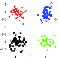
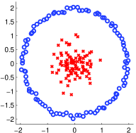
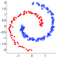
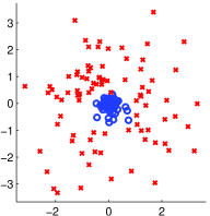
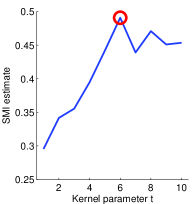
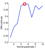
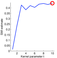
(a) Four Gaussian blobs	(b) Circle & Gaussian	(c) Double spirals	(d) High & low densities

Figure 4: Illustrative examples. Cluster assignments obtained by SMIC (top) and model selection curves obtained by LSMI (bottom).

$\mathrm{ARI}=1$	$\mathrm{ARI}=1$	$\mathrm{ARI}=0.021$	$\mathrm{ARI}=0.173$
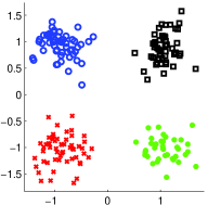
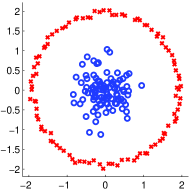
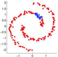
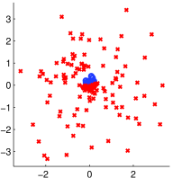
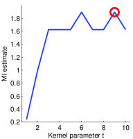
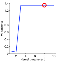
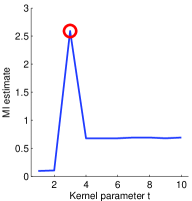
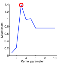
(a) Four Gaussian blobs	(b) Circle & Gaussian	(c) Double spirals	(d) High & low densities

Figure 5: Illustrative examples. Cluster assignments obtained by MIC (top) and model selection curves obtained by MLMI (bottom).

The top graphs in Figure 5 depict the cluster assignments obtained by SMIC with the uniform class-prior, and the bottom graphs in Figure 5 depict the model selection curves obtained by LSMI (i.e., the values of LSMI as functions of the model parameter $t$). The clustering performance was evaluated by the adjusted Rand index (ARI; Hubert and Arabie, 1985) between inferred cluster assignments and the ground truth categories (see Appendix for the details of ARI). Larger ARI values mean better performance, and ARI takes its maximum value $1$ when two sets of cluster assignments are identical. The results show that SMIC combined with LSMI works well for these toy datasets.

Figure 5 depicts the cluster assignments and model selection curves obtained by MIC with MLMI (see Section 3.8), where pre-training of the kernel logistic model using the cluster assignments obtained by self-tuning spectral clustering (Zelnik-Manor and Perona, 2005) was carried out for initializing MIC (Gomes et al., 2010). The figure shows that qualitatively good clustering results were obtained for the datasets (a) and (b). However, for the datasets (c) and (d), poor results were obtained due to local optima of the objective function (20).

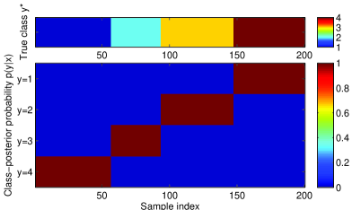
(a) Four Gaussian blobs

(b) Circle & Gaussian

(c) Double spirals

(d) High & low densities

Figure 6: Illustrative examples. Class-posterior probabilities estimated by SMIC.

(a) Four Gaussian blobs

(b) Circle & Gaussian

(c) Double spirals

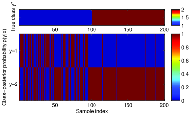
(d) High & low densities

Figure 7: Illustrative examples. Class-posterior probabilities estimated by MIC.

Figure 7 and Figure 7 depict class-posterior probabilities estimated by SMIC and MIC, respectively. The plots show that, for the datasets (a), (b), and (c) where the clusters are clearly separated, the estimated class-posterior probabilities are almost zero-one functions and thus the class prediction is highly certain. On the other hand, for the dataset (d) where the two clusters are overlapped, the estimated class-posterior probabilities tend to take intermediate class-posterior probabilities.

4.2 Influence of Imbalanced Class-Prior Probabilities

Next, we experimentally investigate how imbalanced class-prior probabilities (i.e., the sample size in each cluster is significantly different) influence the clustering performance of SMIC.

We continue using the $4$ artificial datasets used in Section 4.1, but we set the true class-prior probability as

$$p^{\ast}(y=1) =p^{\ast}(y=2)=0.1,0.15,0.2,0.25,$$

$$p^{\ast}(y=3) =p^{\ast}(y=4)=\frac{1-p^{\ast}(y=1)-p^{\ast}(y=2)}{2},$$

for the dataset (a), and

$$p^{\ast}(y=1) =0.2,0.3,0.4,0.5,$$

$$p^{\ast}(y=2) =1-p^{\ast}(y=1),$$

for the datasets (b)–(d). The following $2$ approaches are compared:

SMIC:

SMIC with the uniform class-prior probabilities $\pi_{1}=\pi_{2}=1/2$.

SMIC^∗:

SMIC with the true class-prior probabilities $\pi_{1}=p^{\ast}(y=1)$ and $\pi_{2}=p^{\ast}(y=2)$.

(a) Four Gaussian blobs

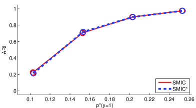
(b) Circle and Gaussian

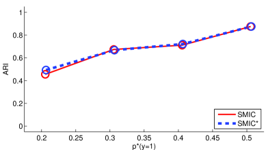
(c) Double spirals

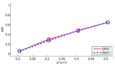
(d) High and low densities

Figure 8: Illustrative examples. The mean ARI over $100$ runs as functions of the class-prior probability $p^{\ast}(y=1)$. The two methods were judged to be comparable in terms of the average ARI by the t-test at the significance level $1\%$.

The mean and standard deviation of ARI over $100$ runs are plotted in Figure 8, showing that the difference between SMIC and SMIC^∗ is negligibly small. Indeed, the two methods were judged to be comparable to each other in terms of the average ARI by the t-test at the significance level $1\%$ for all tested cases. This implies that SMIC is not sensitive to the choice of class-prior probabilities. Thus, in practice, SMIC with the uniform class-prior distribution may be used when the true class-prior is unknown.

4.3 Performance Comparison

Finally, we systematically compare the performance of the proposed and existing clustering methods using various real-world datasets such as images, natural languages, accelerometric sensors, and speech.

4.3.1 Setup

We compared the performance of the following methods, which all do not contain open tuning parameters and therefore experimental results are fair and objective:

KM:

K-means (MacQueen, 1967, see also Section 3.1). We used the software included in the MATLAB Statistics Toolbox, where initial values were randomly generated $100$ times and the best result in terms of the k-means objective value was chosen as the final solution.

SC:

Spectral clustering (Shi and Malik, 2000; Ng et al., 2002, see also Section 3.2) with the self-tuning local-scaling similarity (Zelnik-Manor and Perona, 2005). We used the MATLAB code provided by one of the authors, where the post k-means processing was repeated $10$ times with heuristic initialization: the first center was chosen randomly from samples, and then the next center was iteratively set to the farthest sample from the previous ones. The best result in terms of the k-means objective value out of $10$ repetitions was chosen as the final solution.

MNN:

Mean nearest-neighbor clustering (Faivishevsky and Goldberger, 2010, see also Section 3.7). We used the MATLAB code provided by one of the authors. Following the suggestions provided in the program code, the number of iterations was set to $10$ and the smoothing parameter $\epsilon$ (see Eq.(17)) was set to $\epsilon=1/n$.

MIC:

MI-based clustering with kernel logistic models and the sparse local-scaling kernel (Gomes et al., 2010, see also Section 3.8), where model selection is carried out by maximum-likelihood MI (MLMI; Suzuki et al., 2008). We implemented this method using MATLAB, which is a combination of the MIC code personally provided by one of the authors, and the MLMI code available from the web page of one of the authors. Following the suggestion provided in the original program code, MIC was initialized by pre-training of the kernel logistic model using the cluster assignments obtained by spectral clustering. The tuning parameter $t$ included in the sparse local-scaling kernel (7) was chosen from $\{1,\ldots,10\}$ based on MLMI with Gaussian kernels (see Section 3.8). The Gaussian kernel width in MLMI was chosen from $\{10^{-2},10^{-1.5},10^{-1},\ldots,10^{2}\}$ based on cross-validation. As suggested in the MLMI code provided by the author, the number of kernel bases in MLMI was limited to $200$, which were randomly chosen from all $n$ kernels.

SMIC:

SMI-based clustering with the sparse local-scaling kernel and the uniform class-prior distribution (see Section 2.3), where model selection is carried out by least-squares MI (LSMI; Suzuki et al., 2009, see also Section 2.4). We implemented SMIC and LSMI using MATLAB by ourselves. The tuning parameter $t$ included in the sparse local-scaling kernel (7) was chosen from $\{1,\ldots,10\}$ based on LSMI with Gaussian kernels (see Section 2.4). The Gaussian kernel width and regularization parameter included in LSMI were chosen from $\{10^{-2},10^{-1.5},10^{-1},\ldots,10^{2}\}$ and $\{10^{-3},10^{-2.5},10^{-2},\ldots,10^{1}\}$, respectively, based on cross-validation. Similarly to MLMI, the number of kernel bases in LSMI was limited to $200$, which were randomly chosen from all $n$ kernels.

In addition to the clustering quality in terms of ARI, we also evaluated the computational efficiency of each method by the CPU computation time.

4.3.2 Datasets

We used the following $6$ real-world datasets.

Digit $(d=256,n=5000,~{}\mathrm{and}~{}c=10)$:

The USPS hand-written digit dataset, which contains $9298$ digit images. Each image consists of $256$ $(=16\times 16)$ pixels and represents a digit in $\{0,1,2,\ldots,9\}$. Each pixel takes a value in $[-1,+1]$ corresponding to the intensity level in gray-scale. We randomly chose $500$ samples from each of the $10$ classes, and used $5000$ samples in total.

Face $(d=4096,n=100,~{}\mathrm{and}~{}c=10)$:

The Olivetti Face dataset, which contains $400$ gray-scale face images ($40$ people; $10$ images per person). Each image consists of $4096$ $(=64\times 64)$ pixels and each pixel takes an integer value between $0$ and $255$ as the intensity level. We randomly chose $10$ people, and used $100$ samples in total.

Document $(d=50,n=700,~{}\mathrm{and}~{}c=7)$:

The 20-Newsgroups dataset, which contains $20000$ newsgroup documents across $20$ different newsgroups. We merged the $20$ newsgroups into the following $7$ top-level categories: ‘comp’, ‘rec’, ‘sci’, ‘talk’, ‘alt’, ‘misc’, and ‘soc’. Each document is expressed by a $10000$-dimensional bag-of-words vector of term-frequencies. Following the convention (Joachims, 2002), we transformed the term-frequency vectors to the term frequency/inverse document frequency (TFIDF) vector, i.e., we multiplied the term-frequency by the logarithm of the inverse ratio of the documents containing the corresponding word. We randomly chose $100$ samples from each of the $7$ classes, and used $700$ samples in total. We applied principal component analysis (PCA; Pearson, 1901; Jolliffe, 1986) to the $700$ samples, and extracted $50$-dimensional feature vectors.

Word $(d=50,n=300,~{}\mathrm{and}~{}c=3)$:

The SENSEVAL-2 dataset for word-sense disambiguation. We took the noun ‘interest’ appeared in $1930$ contexts, having $3$ different meanings: ‘advantage, advancement or favor’, ‘a share in a company or business’, and ‘money paid for the use of money’ (i.e., $3$ classes). From each surrounding context, we extracted a $14936$-dimensional feature vector (Niu et al., 2005), which includes three types of features: part-of-speech of neighboring words with position information, bag-of-words in the surrounding context, and local collocation (Lee and Ng, 2002). We randomly chose $100$ samples from each of the $3$ classes, and used $300$ samples in total. We applied PCA to the $300$ samples, and extracted $50$-dimensional feature vectors.

Accelerometry $(d=5,n=300,~{}\mathrm{and}~{}c=3)$:

The ALKAN dataset, which contains $3$-axis (i.e., x-, y-, and z-axes) accelerometric data collected by the iPod touch. In the data collection procedure, subjects were asked to perform three specific tasks: walking, running, and standing up. The duration of each task was arbitrary, and the sampling rate was $20$Hz with small variations. Each data-stream was then segmented in a sliding window manner with window width $5$ seconds and sliding step $1$ second (Hachiya et al., 2011). Depending on subjects, the position and orientation of the accelerometer was arbitrary—held by hand or kept in a pocket or a bag. For this reason, we took the $\ell_{2}$-norm of the $3$-dimensional acceleration vector at each time step, and computed the following $5$ orientation-invariant features from each window: mean, standard deviation, fluctuation of amplitude, average energy, and frequency-domain entropy (Bao and Intille, 2004; Bharatula et al., 2005). We randomly chose $100$ samples from each of the $3$ classes, and used $300$ samples in total.

Speech $(d=50,n=400,~{}\mathrm{and}~{}c=2)$:

An in-house speech dataset, which contains short utterance samples recorded from $2$ male subjects speaking in French with sampling rate $44.1$kHz. From each utterance sample, we extracted a $50$-dimensional line spectral frequencies vector (Kain and Macon, 1988). We randomly chose $200$ samples from each class, and used $400$ samples in total.

For each dataset, the experiment was repeated $100$ times with random choice of samples from the database, where the cluster size is balanced. Samples were centralized and their variance was normalized in the dimension-wise manner, before feeding them to clustering algorithms.

4.3.3 Results

The experimental results are described in Table 1. For the digit dataset, MIC and SMIC outperform KM, SC, and MNN in terms of ARI. The entire computation time of SMIC including model selection is faster than KM, SC, and MIC, and is comparable to MNN which does not include a model selection procedure. For the face dataset, SC, MIC, and SMIC are comparable to each other and are better than KM and MNN in terms of ARI. For the document and word datasets, SMIC tends to outperform the other methods. For the accelerometry dataset, MNN and SMIC work better than the other methods. Finally, for the speech dataset, MIC and SMIC work comparably well, and are significantly better than KM, SC, and MNN.

Table 1: Experimental results on real-world datasets (with equal cluster size). The average clustering accuracy (and its standard deviation in the bracket) in terms of ARI and the average CPU computation time in second over $100$ runs are described. Larger ARI is better, and shorter computation time is preferable. The best method in terms of the average ARI and methods judged to be comparable to the best one by the t-test at the significance level $1\%$ are described in boldface. Computation time of MIC and SMIC corresponds to the time for computing a clustering solution after model selection has been carried out. For references, computation time for the entire procedure including model selection is described in the square bracket, which depends on the number of model candidates (in the current setup, we had $81$ ($=9\times 9$) candidates.

Digit ($d=256,~{}n=5000,~{}\mathrm{and}~{}c=10$)
	KM	SC	MNN	MIC	SMIC
ARI	0.42(0.01)	0.24(0.02)	0.44(0.03)	0.63(0.08)	0.63(0.05)
Time	835.9	973.3	318.5	84.4[3631.7]	14.4[359.5]
Face ($d=4096,~{}n=100,~{}\mathrm{and}~{}c=10$)
	KM	SC	MNN	MIC	SMIC
ARI	0.60(0.11)	0.62(0.11)	0.47(0.10)	0.64(0.12)	0.65(0.11)
Time	93.3	2.1	1.0	1.4[30.8]	0.0[19.3]
Document ($d=50,~{}n=700,~{}\mathrm{and}~{}c=7$)
	KM	SC	MNN	MIC	SMIC
ARI	0.00(0.00)	0.09(0.02)	0.09(0.02)	0.01(0.02)	0.19(0.03)
Time	77.8	9.7	6.4	3.4[530.5]	0.3[115.3]
Word ($d=50,~{}n=300,~{}\mathrm{and}~{}c=3$)
	KM	SC	MNN	MIC	SMIC
ARI	0.04(0.05)	0.02(0.01)	0.02(0.02)	0.04(0.04)	0.08(0.05)
Time	6.5	5.9	2.2	1.0[369.6]	0.2[203.9]
Accelerometry ($d=5,~{}n=300,~{}\mathrm{and}~{}c=3$)
	KM	SC	MNN	MIC	SMIC
ARI	0.49(0.04)	0.58(0.14)	0.71(0.05)	0.57(0.23)	0.68(0.12)
Time	0.4	3.3	1.9	0.8[410.6]	0.2[92.6]
Speech ($d=50,~{}n=400,~{}\mathrm{and}~{}c=2$)
	KM	SC	MNN	MIC	SMIC
ARI	0.00(0.00)	0.00(0.00)	0.04(0.15)	0.18(0.16)	0.21(0.25)
Time	0.9	4.2	1.8	0.7[413.4]	0.3[179.7]

Table 2: Experimental results on real-world datasets under imbalanced setup. ARI values are described in the table. Class-imbalance was realized by setting the sample size of the first class $m$ times larger than other classes. SMIC was computed with the uniform prior (i.e., the non-informative prior). The results for $m=1$ are the same as the ones reported in Table 1.

Digit ($d=256,~{}n=5000,~{}\mathrm{and}~{}c=10$)
	KM	SC	MNN	MIC	SMIC
$m=1$	0.42(0.01)	0.24(0.02)	0.44(0.03)	0.63(0.08)	0.63(0.05)
$m=2$	0.52(0.01)	0.21(0.02)	0.43(0.04)	0.60(0.05)	0.63(0.05)
Document ($d=50,~{}n=700,~{}\mathrm{and}~{}c=7$)
	KM	SC	MNN	MIC	SMIC
$m=1$	0.00(0.00)	0.09(0.02)	0.09(0.02)	0.01(0.02)	0.19(0.03)
$m=2$	0.01(0.01)	0.10(0.03)	0.10(0.02)	0.01(0.02)	0.19(0.04)
$m=3$	0.01(0.01)	0.10(0.03)	0.09(0.02)	-0.01(0.03)	0.16(0.05)
$m=4$	0.02(0.01)	0.09(0.03)	0.08(0.02)	-0.00(0.04)	0.14(0.05)
Word ($d=50,~{}n=300,~{}\mathrm{and}~{}c=3$)
	KM	SC	MNN	MIC	SMIC
$m=1$	0.04(0.05)	0.02(0.01)	0.02(0.02)	0.04(0.04)	0.08(0.05)
$m=2$	0.00(0.07)	-0.01(0.01)	0.01(0.02)	-0.02(0.05)	0.03(0.05)
Accelerometry ($d=5,~{}n=300,~{}\mathrm{and}~{}c=3$)
	KM	SC	MNN	MIC	SMIC
$m=1$	0.49(0.04)	0.58(0.14)	0.71(0.05)	0.57(0.23)	0.68(0.12)
$m=2$	0.48(0.05)	0.54(0.14)	0.58(0.11)	0.49(0.19)	0.69(0.16)
$m=3$	0.49(0.05)	0.47(0.10)	0.42(0.12)	0.42(0.14)	0.66(0.20)
$m=4$	0.49(0.06)	0.38(0.11)	0.31(0.09)	0.40(0.18)	0.56(0.22)

Overall, MIC was shown to work reasonably well, implying that the MLMI-based model selection strategy is practically useful. SMIC was shown to work even better than MIC, with much less computation time. The accuracy improvement of SMIC over MIC was gained by computing the SMIC solution in a closed-form without any heuristic initialization. The computational efficiency of SMIC was brought by the analytic computation of the optimal solution and the class-wise optimization of LSMI (see Section 2.4).

The performance of MNN and SC was rather unstable because of the heuristic averaging of the number of nearest neighbors in MNN and the heuristic choice of local scaling in SC. In terms of computation time, they are relatively efficient for small- to medium-sized datasets, but they are expensive for the largest dataset, digit. KM was not reliable for the document and speech datasets because of the restriction that the cluster boundaries are linear. For the digit, face, and document datasets, KM was computationally very expensive since a large number of iterations were needed until convergence to a local optimum solution.

Finally, we performed similar experiments under imbalanced setup, where the sample size of the first class was set to be $m$ times larger than other classes with the total number of samples fixed to the same number. The results are summarized in Table 2, showing that the performance of all methods tends to be degraded as the degree of cluster imbalance increases. Thus, clustering becomes more challenging if the cluster size is imbalanced. Among the compared methods, the proposed SMIC (with the uniform prior) still worked better than other methods.

Overall, the proposed SMIC combined with LSMI was shown to be a useful alternative to existing clustering approaches.

5 Conclusions

In this paper, we proposed a novel information-maximization clustering method that learns class-posterior probabilities in an unsupervised manner so that the squared-loss mutual information (SMI) between feature vectors and cluster assignments is maximized. The proposed algorithm, called SMI-based clustering (SMIC), allows us to obtain clustering solutions analytically by solving a kernel eigenvalue problem. Thus, unlike the previous information-maximization clustering methods (Agakov and Barber, 2006; Gomes et al., 2010), SMIC does not suffer from the problem of local optima. Furthermore, we proposed to use an optimal non-parametric SMI estimator called least-squares mutual information (LSMI) for data-driven parameter optimization. Through experiments, SMIC combined with LSMI was demonstrated to compare favorably with existing clustering methods.

In experiments, the proposed clustering method was shown to be useful for various types of data. However, the amount of improvement is large for some datasets, while it is mild for other datasets. It is thus practically important to have more insights on in what case the proposed method is advantageous.

The sparse local-scaling kernel (7) was shown to be useful in experiments. Since this produces a sparse kernel matrix, the computation of SMIC (i.e., solving a kernel eigenvalue problem) can be carried out very efficiently. However, if model selection is taken into account, the proposed clustering procedure is still computationally rather demanding due to the repeated computation of LSMI, which requires to solve a system of linear equations. In the experiments, we used the Gaussian kernel (11) for LSMI and found it useful in practice. However, it produces a dense kernel matrix and thus a dense system of linear equations need to be solved, which is computationally expensive. If a sparse kernel is used also for LSMI, its computational efficiency will be highly improved. In our preliminary experiments, the use of the sparse local-scaling kernel for LSMI improved the computational efficiency, but it did not perform as well as the Gaussian kernel. Thus, our important future work is to find a sparse kernel that gives an accurate approximation of SMI with high computational efficiency.

As addressed in Song et al. (2007), kernelized methods can be applied to clustering of non-vectorial structured objects such as strings, trees, and graphs by employing kernel functions defined for such structured data (Lodhi et al., 2002; Duffy and Collins, 2002; Kashima and Koyanagi, 2002; Kondor and Lafferty, 2002; Kashima et al., 2003; Gärtner et al., 2003; Gärtner, 2003). Since these structured kernels usually contain tuning parameters, the performance of clustering methods without systematic model selection strategies depends on subjective parameter tuning, which is not preferable in practice. For Gaussian kernels, there exists a popular heuristic that the Gaussian width is set to the median distance between samples (Fukumizu et al., 2009). However, there seems no such common heuristic for structured kernels. In such scenarios, the proposed method will be highly advantageous because it allows systematic model selection for any kernels. We will explore this direction in our future work.

We experimentally showed that the proposed method with the uniform class-prior distribution still works reasonably well even when the true class-prior probability is not uniform. This is a useful property in practice since the true class-prior probability is often unknown. Another way to address this issue is to estimate the true class-prior probability in a data-driven fashion, for example, iteratively performing clustering and updating the class-prior probabilities. We will investigate such an adaptive approach in our future work.

The proposed method uses SMI as the common guidance for clustering, although we are using two SMI approximators: $\widehat{\mathrm{SMI}}$ defined by Eq.(8) for finding clustering solutions and $\mathrm{LSMI}$ defined by Eq.(14) for selecting models. Since $\widehat{\mathrm{SMI}}$ does not explicitly include cluster labels $\{y_{i}\}_{i=1}^{n}$, it has a simple form and therefore is suited for efficient maximization. Indeed, we can obtain an optimal solution analytically by solving an eigenvalue problem. However, since $\widehat{\mathrm{SMI}}$ is an unsupervised estimator where the cluster labels $\{y_{i}\}_{i=1}^{n}$ are not used, it may not be accurate enough for model selection purposes. Indeed, our preliminary experiments showed that the use of $\widehat{\mathrm{SMI}}$ is not appropriate as a model selection criterion. On the other hand, since $\mathrm{LSMI}$ achieves the optimal non-parametric convergence rate, its high accuracy is suitable for model selection purposes. However, LSMI explicitly requires cluster labels $\{y_{i}\}_{i=1}^{n}$ and thus is not suited for efficient maximization. Based on the optimality of LSMI, we ideally want to use LSMI consistently for both finding clustering solutions and selecting models. However, its optimization involves discrete optimization of $\{y_{i}\}_{i=1}^{n}$, which is cumbersome in practice. Our future challenge is to develop a practical clustering algorithm based directly on LSMI.

Appendix: Rand Index and Adjusted Rand Index

Here, we review the definitions of the Rand index (RI; Rand, 1971) and the adjusted Rand index (ARI; Hubert and Arabie, 1985), which are used for evaluating the quality of clustering results. Let $\{y_{i}^{*}\}_{i=1}^{n}$ be the ground-truth cluster assignments, and let $\{y_{i}\}_{i=1}^{n}$ be a clustering solution obtained by some algorithm. The goal is to quantitatively evaluate the similarity between $\{y_{i}\}_{i=1}^{n}$ and $\{y_{i}^{*}\}_{i=1}^{n}$.

Table 3: Notation for Rand index and adjusted Rand index.

(a)	(b)
${\mathcal{C}}_{1}^{*}$ $\cdots$ ${\mathcal{C}}_{c}^{*}$ Sum ${\mathcal{C}}_{1}$ $n_{1,1}$ $\cdots$ $n_{1,c}$ $n_{1}$ $\vdots$ $\vdots$ $\ddots$ $\vdots$ $\vdots$ ${\mathcal{C}}_{c}$ $n_{c,1}$ $\cdots$ $n_{c,c}$ $n_{c}$ Sum $n_{1}^{*}$ $\cdots$ $n_{c}^{*}$ $n$	Pairs in $\{{\mathcal{C}}_{y^{\prime}}^{*}\}_{y^{\prime}=1}^{c}$ Same Different Pairs in Same $m_{{\mathcal{C}},{\mathcal{C}}^{*}}$ $m_{{\mathcal{C}},\bar{{\mathcal{C}}}^{*}}$ $\{{\mathcal{C}}_{y}\}_{y=1}^{c}$ Different $m_{\bar{{\mathcal{C}}},{\mathcal{C}}^{*}}$ $m_{\bar{{\mathcal{C}}},\bar{{\mathcal{C}}}^{*}}$

The most direct way to evaluate the discrepancy between $\{y_{i}\}_{i=1}^{n}$ and $\{y_{i}^{*}\}_{i=1}^{n}$ would be to naively verify the correctness of the predicted labels. However, in clustering, predicted class labels $\{y_{i}\}_{i=1}^{n}$ do not have to be equal to the true labels $\{y_{i}^{*}\}_{i=1}^{n}$, but only their partition matters. The correctness of the partition may be evaluated by verifying the correctness of the predicted labels for all possible label permutations. However, this is computationally expensive if the number of classes is large. RI and ARI are alternative performance measures that can overcome this computational problem in a systematic way.

For the two partitions $\{y_{i}\}_{i=1}^{n}$ and $\{y_{i}^{*}\}_{i=1}^{n}$, let ${\mathcal{C}}_{y}$ and ${\mathcal{C}}_{y}^{*}$ ($y=1,\ldots,c$) be sets of indices of samples in cluster $y$, respectively:

$${\mathcal{C}}_{y} =\{y_{i}\;|\;y_{i}=y\},$$

$${\mathcal{C}}_{y}^{*} =\{y_{i}^{*}\;|\;y_{i}^{*}=y\}.$$

Let $n_{y,y^{\prime}}$ be the number of samples that are assigned to the cluster ${\mathcal{C}}_{y}$ and the cluster ${\mathcal{C}}_{y^{\prime}}^{*}$. Let $n_{y}$ (resp. $n_{y}^{*}$) be the number of samples that are assigned to the cluster ${\mathcal{C}}_{y}$ (resp. ${\mathcal{C}}_{y^{\prime}}^{*}$). The notation is summarized in Table 3(a).

Let $m_{{\mathcal{C}},{\mathcal{C}}^{*}}$, $m_{{\mathcal{C}},\bar{{\mathcal{C}}}^{*}}$, $m_{\bar{{\mathcal{C}}},{\mathcal{C}}^{*}}$, and $m_{\bar{{\mathcal{C}}},\bar{{\mathcal{C}}}^{*}}$ be defined as

$$m_{{\mathcal{C}},{\mathcal{C}}^{*}} :=\sum_{y,y^{\prime}=1}^{c}\begin{pmatrix}n_{y,y^{\prime}}\\ 2\\ \end{pmatrix},$$

$$m_{{\mathcal{C}},\bar{{\mathcal{C}}}^{*}} :=\sum_{y=1}^{c}\begin{pmatrix}n_{y}\\ 2\\ \end{pmatrix}-m_{{\mathcal{C}},{\mathcal{C}}^{*}},$$

$$m_{\bar{{\mathcal{C}}},{\mathcal{C}}^{*}} :=\sum_{y^{\prime}=1}^{c}\begin{pmatrix}n_{y^{\prime}}^{*}\\ 2\\ \end{pmatrix}-m_{{\mathcal{C}},{\mathcal{C}}^{*}},$$

$$m_{\bar{{\mathcal{C}}},\bar{{\mathcal{C}}}^{*}} :=\begin{pmatrix}n\\ 2\\ \end{pmatrix}-m_{{\mathcal{C}},{\mathcal{C}}^{*}}-m_{{\mathcal{C}},\bar{{\mathcal{C}}}^{*}}-m_{\bar{{\mathcal{C}}},{\mathcal{C}}^{*}},$$

where $m_{{\mathcal{C}},{\mathcal{C}}^{*}}$ denotes the number of pairs of samples that are assigned to the same cluster both in $\{{\mathcal{C}}_{y}\}_{y=1}^{c}$ and $\{{\mathcal{C}}_{y^{\prime}}^{*}\}_{y^{\prime}=1}^{c}$, $m_{{\mathcal{C}},\bar{{\mathcal{C}}}^{*}}$ denotes the number of pairs of samples that are assigned to the same cluster in $\{{\mathcal{C}}_{y}\}_{y=1}^{c}$ but are assigned to different clusters in $\{{\mathcal{C}}_{y^{\prime}}^{*}\}_{y^{\prime}=1}^{c}$, $m_{\bar{{\mathcal{C}}},{\mathcal{C}}^{*}}$ denotes the number of pairs of samples that are assigned to the same cluster in $\{{\mathcal{C}}_{y^{\prime}}^{*}\}_{y^{\prime}=1}^{c}$ but are assigned to different clusters in $\{{\mathcal{C}}_{y}\}_{y=1}^{c}$, and $m_{\bar{{\mathcal{C}}},\bar{{\mathcal{C}}}^{*}}$ denotes the number of pairs of samples that are assigned to different clusters both in $\{{\mathcal{C}}_{y}\}_{y=1}^{c}$ and $\{{\mathcal{C}}_{y^{\prime}}^{*}\}_{y^{\prime}=1}^{c}$. $m_{{\mathcal{C}},{\mathcal{C}}^{*}}+m_{\bar{{\mathcal{C}}},\bar{{\mathcal{C}}}^{*}}$ can be considered as the number of ‘agreements’ between $\{{\mathcal{C}}_{y}\}_{y=1}^{c}$ and $\{{\mathcal{C}}_{y^{\prime}}^{*}\}_{y^{\prime}=1}^{c}$, while $m_{{\mathcal{C}},\bar{{\mathcal{C}}}^{*}}+m_{\bar{{\mathcal{C}}},{\mathcal{C}}^{*}}$ can be regarded as the number of ‘disagreements’ between $\{{\mathcal{C}}_{y}\}_{y=1}^{c}$ and $\{{\mathcal{C}}_{y^{\prime}}^{*}\}_{y^{\prime}=1}^{c}$. The notation is summarized in Table 3(b).

The Rand index (RI; Rand, 1971) is defined and expressed as

$$\mathrm{RI} :=\frac{m_{{\mathcal{C}},{\mathcal{C}}^{*}}+m_{\bar{{\mathcal{C}}},\bar{{\mathcal{C}}}^{*}}}{m_{{\mathcal{C}},{\mathcal{C}}^{*}}+m_{{\mathcal{C}},\bar{{\mathcal{C}}}^{*}}+m_{\bar{{\mathcal{C}}},{\mathcal{C}}^{*}}+m_{\bar{{\mathcal{C}}},\bar{{\mathcal{C}}}^{*}}}$$

$$\phantom{:}=(m_{{\mathcal{C}},{\mathcal{C}}^{*}}+m_{\bar{{\mathcal{C}}},\bar{{\mathcal{C}}}^{*}})\Big{/}\begin{pmatrix}n\\ 2\\ \end{pmatrix}.$$

The Rand index lies between $0$ and $1$, and takes $1$ if the two clustering solutions $\{{\mathcal{C}}_{y}\}_{y=1}^{c}$ and $\{{\mathcal{C}}_{y^{\prime}}^{*}\}_{y^{\prime}=1}^{c}$ agree with each other perfectly.

A potential drawback of the Rand index is that its expected value is not a constant (say, $0$) if two clustering solutions are completely random. To overcome this problem, the adjusted Rand index (ARI) was proposed (Hubert and Arabie, 1985). ARI is defined as

$$\mathrm{ARI}:=\frac{m_{{\mathcal{C}},{\mathcal{C}}^{*}}+m_{\bar{{\mathcal{C}}},\bar{{\mathcal{C}}}^{*}}-\mu}{m_{{\mathcal{C}},{\mathcal{C}}^{*}}+m_{{\mathcal{C}},\bar{{\mathcal{C}}}^{*}}+m_{\bar{{\mathcal{C}}},{\mathcal{C}}^{*}}+m_{\bar{{\mathcal{C}}},\bar{{\mathcal{C}}}^{*}}-\mu}.$$

$\mu$ is the expected value of $m_{{\mathcal{C}},{\mathcal{C}}^{*}}+m_{\bar{{\mathcal{C}}},\bar{{\mathcal{C}}}^{*}}$:

$$\mu:=\mathbb{E}\left[m_{{\mathcal{C}},{\mathcal{C}}^{*}}+m_{\bar{{\mathcal{C}}},\bar{{\mathcal{C}}}^{*}}\right],$$

where $\mathbb{E}$ denotes the expectation over cluster assignments. ARI takes the maximum value $1$ when two sets of cluster assignments are identical, and takes $0$ if the index equals its expected value.

Under the assumption that the clustering solutions $\{{\mathcal{C}}_{y}\}_{y=1}^{c}$ and $\{{\mathcal{C}}_{y^{\prime}}^{*}\}_{y^{\prime}=1}^{c}$ are randomly drawn from a generalized hyper-geometric distribution, it holds that

$$\mathbb{E}\left[m_{{\mathcal{C}},{\mathcal{C}}^{*}}\right] =(m_{{\mathcal{C}},{\mathcal{C}}^{*}}+m_{{\mathcal{C}},\bar{{\mathcal{C}}}^{*}})(m_{{\mathcal{C}},{\mathcal{C}}^{*}}+m_{\bar{{\mathcal{C}}},{\mathcal{C}}^{*}})\Big{/}\begin{pmatrix}n\\ 2\\ \end{pmatrix},$$

$$\mathbb{E}\left[m_{\bar{{\mathcal{C}}},\bar{{\mathcal{C}}}^{*}}\right] =(m_{{\mathcal{C}},\bar{{\mathcal{C}}}^{*}}+m_{\bar{{\mathcal{C}}},\bar{{\mathcal{C}}}^{*}})(m_{\bar{{\mathcal{C}}},{\mathcal{C}}^{*}}+m_{\bar{{\mathcal{C}}},\bar{{\mathcal{C}}}^{*}})\Big{/}\begin{pmatrix}n\\ 2\\ \end{pmatrix}.$$

Then ARI can be expressed as

$$\mathrm{ARI}=\frac{\displaystyle\begin{pmatrix}n\\ 2\\ \end{pmatrix}\sum_{y,y^{\prime}=1}^{c}\begin{pmatrix}n_{y,y^{\prime}}\\ 2\\ \end{pmatrix}-\sum_{y=1}^{c}\begin{pmatrix}n_{y}\\ 2\\ \end{pmatrix}\sum_{y^{\prime}=1}^{c}\begin{pmatrix}n_{y^{\prime}}^{*}\\ 2\\ \end{pmatrix}}{\displaystyle\frac{1}{2}\begin{pmatrix}n\\ 2\\ \end{pmatrix}\left[\sum_{y=1}^{c}\begin{pmatrix}n_{y}\\ 2\\ \end{pmatrix}+\sum_{y^{\prime}=1}^{c}\begin{pmatrix}n_{y^{\prime}}^{*}\\ 2\\ \end{pmatrix}\right]-\sum_{y=1}^{c}\begin{pmatrix}n_{y}\\ 2\\ \end{pmatrix}\sum_{y^{\prime}=1}^{c}\begin{pmatrix}n_{y^{\prime}}^{*}\\ 2\\ \end{pmatrix}}.$$

Note that RI and ARI can be defined even when two sets of cluster assignments $\{y_{i}\}_{i=1}^{n}$ and $\{y_{i}^{*}\}_{i=1}^{n}$ have different numbers of clusters, i.e., $\{{\mathcal{C}}_{y}\}_{y=1}^{c}$ and $\{{\mathcal{C}}_{y^{\prime}}^{*}\}_{y^{\prime}=1}^{c^{\prime}}$ with $c\neq c^{\prime}$. This is highly convenient in practice since, when the number of true clusters is large, clustering algorithms often produce clustering solutions with a smaller number of clusters (i.e., some of the clusters have no samples). Even in such cases, RI and ARI can still be used for evaluating the quality of clustering solutions.

References

- Agakov and Barber (2006) F. Agakov and D. Barber. Kernelized infomax clustering. In Y. Weiss, B. Schölkopf, and J. Platt, editors, Advances in Neural Information Processing Systems 18, pages 17–24. MIT Press, Cambridge, MA, USA, 2006.
- Ali and Silvey (1966) S. M. Ali and S. D. Silvey. A general class of coefficients of divergence of one distribution from another. Journal of the Royal Statistical Society, Series B, 28(1):131–142, 1966.
- Aloise et al. (2009) D. Aloise, A. Deshpande, P. Hansen, and P. Popat. NP-hardness of Euclidean sum-of-squares clustering. Machine Learning, 75(2):245–249, 2009.
- Amari (1967) S. Amari. Theory of adaptive pattern classifiers. IEEE Transactions on Electronic Computers, EC-16(3):299–307, 1967.
- Andrieu et al. (2003) C. Andrieu, N. de Freitas, A. Doucet, and M.l I. Jordan. An introduction to MCMC for machine learning. Machine Learning, 50(1-2):5–43, 2003.
- Antoniak (1974) C. Antoniak. Mixtures of Dirichlet processes with applications to Bayesian nonparametric problems. The Annals of Statistics, 2(6):1152–1174, 1974.
- Aronszajn (1950) N. Aronszajn. Theory of reproducing kernels. Transactions of the American Mathematical Society, 68:337–404, 1950.
- Attias (2000) H.i Attias. A variational Baysian framework for graphical models. In S. A. Solla, T. K. Leen, and K.-R. Müller, editors, Advances in Neural Information Processing Systems 12, pages 209–215. MIT Press, 2000.
- Bach and Harchaoui (2008) F. Bach and Z. Harchaoui. DIFFRAC: A discriminative and flexible framework for clustering. In J. C. Platt, D. Koller, Y. Singer, and S. Roweis, editors, Advances in Neural Information Processing Systems 20, pages 49–56. MIT Press, Cambridge, MA, USA, 2008.
- Bach and Jordan (2006) F. Bach and M. I. Jordan. Learning spectral clustering, with application to speech separation. Journal of Machine Learning Research, 7:1963–2001, 2006.
- Bao and Intille (2004) L. Bao and S. S. Intille. Activity recognition from user-annotated acceleration data. In Proceedings of 2nd IEEE International Conference on Pervasive Computing, pages 1–17, 2004.
- Bharatula et al. (2005) N. B. Bharatula, M. Stager, P. Lukowicz, and G. Troster. Empirical study of design choices in multi-sensor context ecognition. In Proceedings of International Forun on Applied Wearable Computing, pages 79–93, 2005.
- Bishop (2006) C. M. Bishop. Pattern Recognition and Machine Learning. Springer, New York, NY, USA, 2006.
- Blei and Jordan (2006) D. M. Blei and M. I. Jordan. Variational inference for Dirichlet process mixtures. Bayesian Analysis, 1(1):121–144, 2006.
- Carreira-Perpiñán (2006) M. Á. Carreira-Perpiñán. Fast nonparametric clustering with Gaussian blurring mean-shift. In W. Cohen and A. Moore, editors, Proceedings of 23rd International Conference on Machine Learning (ICML2006), pages 153–160, Pittsburgh, PA, Jun. 25–29 2006.