Connectivity of edge and surface states in topological insulators

Abstract

The edge states of a two-dimensional quantum spin Hall (QSH) insulator form a one-dimensional helical metal which is responsible for the transport property of the QSH insulator. Conceptually, such a one-dimensional helical metal can be attached to any scattering region as the usual metallic leads. We study the analytical property of the scattering matrix for such a conceptual multiterminal scattering problem in the presence of time reversal invariance. As a result, several theorems on the connectivity property of helical edge states in two-dimensional QSH systems as well as surface states of three-dimensional topological insulators are obtained. Without addressing real model details, these theorems, which are phenomenologically obtained, emphasize the general connectivity property of topological edge/surface states from the mere time reversal symmetry restriction.

I introduction

Time reversal symmetry (TRS) has profound and sometimes mysterious consequences in quantum physics. Recently, in the frontier of condensed matter physics, the exciting development of two-dimensional (2D) and three-dimensional (3D) topological insulators (TIs)Qi_2010 ; kane marks a new depth of our understanding of TR in the quantum exploration of the material world. The TI materials have strong spin-orbital coupling (SOC) while maintaining TRS. Prominently, these materials are characterized by a nontrivial band structure with gapped bulk spectrum while their edge excitations are gapless. Among divergent research activities in this field, the theoretical proposal of 2D quantum spin Hall (QSH) insulatorsKane1 ; Kane2 ; Bernevig_2006_PRL ; Bernevig_2006 and the experimental confirmationKonig_2007 ; A.Roth are of core importance to the whole field. For our purpose, we would like to point out especially that the nonlocal transport measurement has confirmed that the transport property of a 2D QSH insulator is dominated by helical edge states near its edgesA.Roth .

Different from the traditional integer quantum Hall system, where TRS is broken by a magnetic field and the edge states are chiral, the edge states in the QSH system are helical, which are composed of pairs of counter-propagating modes with opposite spin polarizations. For each pair, the two branches of states transform into each other under a TR transformation. Due to their conducting property, such helical edge states are called the helical liquidCongjun Wu . In the 2D QSH phase, the helical states are localized near edges and separated spatially by the gapped bulk region. In this paper, we dub the phrase helical metal to refer to the one-dimensional (1D) metal for which the low-energy dispersion is characterized by a pair of helical edge states. Such 1D helical metals are isolated from each other by a macroscopic distance (e.g., the width of the Hall bar sample).

The Landauer-Buttiker theory (LBT) is one of the most important frameworks for analyzing the transport property of mesoscopic systemsDatta . In the LBT, the transport process is treated as a quantum scattering problem where the connection between the carrier reservoir (electrical contacts) and the mesoscopic system (scattering region) is modeled as semi-infinite metallic leads. The central quantity in LBT is the scattering matrix, which can be different by using different leads. In practice, the metallic leads can be described by an arbitrary single-particle Hamiltonian with some propagating modes for a given Fermi energy.

In this paper, we will conceptually use the fore-mentioned helical metals as metallic leads and attach them to the central scattering region. For such a conceptual scattering problem, we find that TRS imposes a strong restriction on the form of the scattering matrix. Then, the condition of a physically realizable scattering problem is obtained in Theorem A. This restriction has profound consequences on the connectivity property of edge states. Based on it, we discuss the connectivity properties for edge states in the 2D QSH system (embodied in Theorem B) as well as the surface Dirac cone in the 3D TI (Theorem C). Several discussions for these theorems are provided.

II scattering matrix with helical metal as leads

To begin with, let us consider a system with TRS which is attached with two half-infinite helical metals at its left and right sides. At energy $E$, the left lead has two eigenstates, denoted as $|1s\rangle_{L}$ and $|\bar{1}\bar{s}\rangle_{L}$, while the right lead has eigenstates $|\bar{1}s\rangle_{R}$ and $|1\bar{s}\rangle_{R}$, where 1 refers to right-moving and $\bar{1}$ to left-moving and $s$,$\bar{s}$ are two spin polarizations with respect to some spin quantization axis. Two such states form a Kramers’s pair in each lead, so that they change to each other under time reversal operation $T$. By a proper energy-dependent U(1) gauge fixing, the two states satisfy

$$T|1s\rangle_{L} = |\bar{1}\bar{s}\rangle_{L},T|\bar{1}\bar{s}\rangle_{L}=-|1s\rangle_{L}$$

$$T|\bar{1}s\rangle_{R} = |1\bar{s}\rangle_{R},T|1\bar{s}\rangle_{R}=-|\bar{1}s\rangle_{R}$$ (1)

Through the above equation, $T^{2}=-1$ is respected for spin-1/2 particles. In general, the spin quantization axis as well as wave vectors for the eigenstates is different for the two leads.

For the scattering problem, we generally assume the wave functions on the two leads as:

$$|\psi\rangle_{L} = \phi^{in}_{Ls}|1s\rangle_{L}+\phi^{out}_{L\bar{s}}|\bar{1}\bar{s}\rangle_{L}$$

$$|\psi\rangle_{R} = \phi^{out}_{R\bar{s}}|1\bar{s}\rangle_{R}+\phi^{in}_{Rs}|\bar{1}s\rangle_{R}$$ (2)

in which $\phi^{in}_{Ls}$, $\phi^{in}_{Rs}$ are incident wave amplitudes and $\phi^{out}_{L\bar{s}}$, $\phi^{out}_{R\bar{s}}$ are outgoing amplitudes. It is convenient to introduce the incident wave vector $a=(\phi^{in}_{Ls},\phi^{in}_{Rs})^{T}$ and the outgoing wave vector $b=(\phi^{out}_{L\bar{s}},\phi^{out}_{R\bar{s}})^{T}$. In the standard scattering problem, the scattering matrix $S$ can be defined so that we have $b=Sa$. Due to particle number conservation, $S$ must be a unitary matrix with a proper normalizationDatta , so that $S^{{\dagger}}S=1$, from which we can get $a^{*}=S^{T}b^{*}$. Now let us consider the consequence of TRS. From Eq. (1), we know that under $T$: $a\Rightarrow a^{\prime}=Ta=-b^{*}$, $b\Rightarrow b^{\prime}=Tb=a^{*}$ and $S^{\prime}=TST^{-1}=S$. Thus we have $a^{*}=-Sb^{*}$. Putting these pieces together, we get the following antisymmetry condition for the scattering matrix:

$$S^{T}=-S.$$ (3)

This is a strong restriction on the form of the scattering matrix due to the existence of TRS for the whole system. It turns out that a lot of interesting results can be derived from this property. Now let us discuss them as follows.

First, from the antisymmetry property and the unitarity condition, we can conclude that $S=\left(\begin{array}[]{cc}0&e^{i\phi}\\ -e^{i\phi}&0\\ \end{array}\right).$ Here $\phi$ is a real phase. This result indicates that near the edge of a QSH system, the helical state has no back scattering without $T$-breaking barrier or impurities, which is a well-known propertyQi_2010 . We may interpret this result in the connectivity property of helical states: any $T$-invariant barrier or impurities can not break the connectivity of helical states.

Second, following the same procedure, the derivation of Eq. (3) can be easily extended to the case with an arbitrary number, say $n$, of helical metal leads attached to the central region, with each lead again characterized by one pair of helical states. As a mathematical fact, the determinant of an antisymmetric matrix of odd dimension is zero, i.e., $\det(S)=0$ when $n$ is odd. Consequently, for that case, $S$ can not be a unitary matrix, which is one of the very assumptions that leads us to Eq. (3). To note, the unitarity property of the scattering matrix is the direct consequence of the conservation law of the particle number. What is the meaning of such a logical contradiction? In the above conceptual scattering problem model, we have assumed that $n$ helical metal leads are attached to the central region and thus form a standard multiterminal scattering problem. While the helical states near two edges of a QSH system are separated spatially by the gapped bulk region, which encouraged us to coin the concept of ”helical metal” for the conducting edge, they are actually topologically correlated. The above logical contradiction means the impossibility of a reasonable scattering matrix in a conceptual scattering problem with an odd number of helical leads. Based on these analysis, we can state the following theorem:

Theorem A : In a physical scattering problem with TRS, any central region allows only an even number of helical metals (each with a single pair of helical states) as conduction leads attached upon it.

It can also be straightforwardly shown that the possible existence of any normal leads (which, by definition, must be composed of an even number of helical pair states) in the conceptual scattering problem does not change the statement in Theorem A. It is noteworthy that a related theorem was given by Wu et al.Congjun Wu , in which they proved that the helical metal can not be realized in 1D lattice models with TRS, which is termed a no-go theorem. It turns out that this no-go theorem is a direct consequence of Theorem A: if we can construct a 1D model to be a helical metal, then such a helical metal will become a physical system by itself (instead of being an edge subsystem of another system). So, we can use it as a single independent lead to attach to a TRS central region, which contradicts Theorem A. Physically, Theorem A and the no-go theorem have a common origin, i.e., both of them are a direct consequence of TRS. However, being expressed in the scattering language, Theorem A is more flexible to use. Since only the parity of the number of pairs of helical states matters, from now on, we can loosen the previous definition of helical metal such that their energy spectrums are characterized by any odd number(instead of just one) of helical states. Through Theorem A, we will be able to prove several rigorous properties in the following.

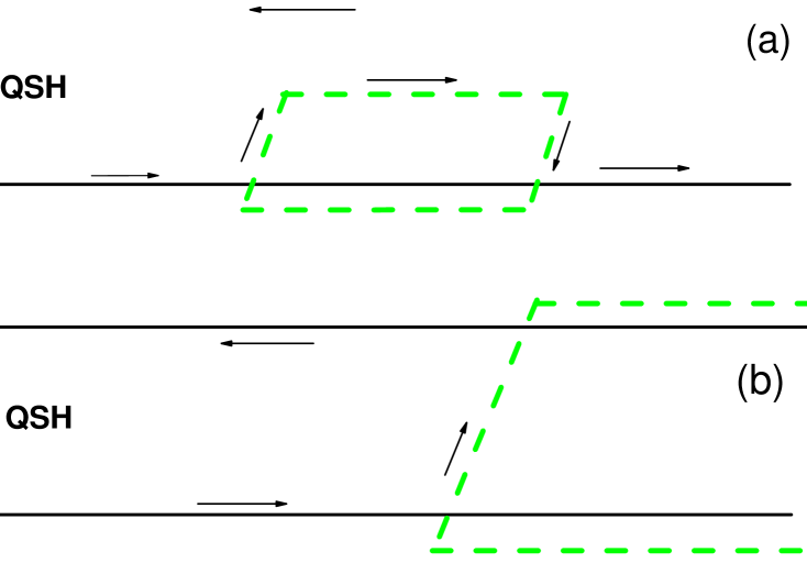
Figure 1: (Color online) 2D QSH states and helical edge states in a stripe geometry. (Black arrows denote propagating direction for one state of the edge helical pair). The band insulator (bordered by green dashed lines) is put on the QSH strip (a) on one edge and (b) bridging two edges.

III connectivity property of edge/surface states of the 2D/3D topological insulators

First, let us consider the 2D QSH system. We will prove that all helical metals should be connected and form a closed loop in a finite system. This result is quite easy to prove starting from Theorem A. Suppose there is a section of line $ab$ (with two ends $a$ and $b$),which is made of helical metal and one of its two ends, say $a$, does not belong to, or, is not connected with, any other section of line which is also a helical metal. If such an end $a$ is chosen to be the central region of the conceptual scattering problem, then, there is only one helical metal attached to $a$, which is contrary to Theorem A. Therefore, we can conclude that this can not physically happen. In Fig. 1(a), we show that the helical state at one edge of the QSH system can circumvent any barrier with TRS and transmit to the other side. If the barrier is chosen to be an insulator under which a forbidden region is defined, the perfect transmission happens by a new helical edge formed around the boundary of the barrier [as shown in Fig. 1(a)]. Furthermore, if the barrier is large enough to bridge the two edges as shown in Fig. 1(b), the helical states from one edge will connect to the other side through the interface between the QSH system and the barrier. From the above discussion, it can be known clearly that there are always helical states near the boundary along which we cut the QSH system. We can summarize this result in the following theorem:

Theorem B:Along any edge of a 2D QSH system or a boundary between a 2D TI and a band insulator, there is always an odd number of pairs of helical states.

Particularly, Theorem B implies the $Z_{2}$ connectivity(evenness/oddness of the number pair of helical states) property between the adjacent edges of any finite 2D QSH sample. For further illustration, let us address the graphene stripe with an intrinsic SOCKane1 ; Kane2 as an example. It is well known that a graphene stripe with zigzag edges has zero-energy flat bands near the zigzag edgesflatzigzag . In the presence of an intrinsic SOC, a bulk gap will open and these flat bands will evolve into helical edge statesKane1 ; Kane2 . However, for a graphene stripe with armchair edges without any SOC, there are no such flat bands. By mere expectation through a continuity consideration, we may anticipate that there are no helical edge states with the inclusion of an intrinsic SOC. However, from Theorem B, we can predict helical edge states also exist near armchair edges, which is in consistent with numerical resultsRuibao Tao .

The famous bulk-edge correspondence theorem in the quantum Hall effect states that the nontrivial topological band structure will ensure the existence of conducting edge modes along system edges, with the number of edge modes determined by the topological Chern number of the filled bandsHatsugai_PRB_1993 . This theorem is generalized with limited success to the QSH caseQi_2006 , which involves sophisticated topological analysis. Theorem B is a direct consequence of the much sought-for bulk-edge correspondence theorem for 2D QSH systems, where only the parity of the number of edge states is important. Our approach leading to Theorem B, though somewhat phenomenological (see discussion below), is model-independent and general. Furthermore, it can be extended to 3D TIs as discussed below.

Figure 2: 3D TI in a pipe geometry with translationally invariant cross section. The local coordination for the wave vector is drawn for the front and the top faces. If the low-energy Hamiltonian of the front face is characterized by a single Dirac Cone, how many Dirac cones are on the top surface?

Now let us turn to the 3D TI, which has also been firmly established both theoretically and experimentallyLFu ; LFu2007PRB ; HZhang ; DHsieh ; DHsieh2009 . As depicted in Fig. 2, we will consider an infinitely long rectangular column composed of a 3D TI. The system is translationally invariant in the $x$ direction. The size of its rectangular cross section is of macroscopic scale so that the quantum confinement effect can be neglected in our discussion. As is well known, a 3D TI is characterized by bulk gap and mid-gap surface excitations. Now, let us assume that the front face is characterized by a single surface Dirac cone (e.g., in $Bi_{2}Te_{3}$) around the center of the Brillouin Zone ($\Gamma$ point). In the following, we shall prove that the top face is also characterized by an odd number of Dirac cones. Let us denote the wave vector $k_{x},k_{y}$ for the front face and $k_{x}^{\prime},k_{y}^{\prime}$ for the top face (as the local coordinate frames drawn in Fig. 2). Since the system is translationally invariant in $x$ direction, $k_{x}$ and $k_{x}^{\prime}$ are good quantum numbers. On the other hand, we can linearly combine the degenerate states with different $k_{y}$ (or $k_{y}^{\prime}$) and use the proper boundary condition to obtain the wave function around the perimeter of the cross section. The geometrical edge between the front and the top face can be regarded as a scattering region for each $k_{x}$-fixed subspace, thus we have a conceptual scattering problem. At a general $E$, we have surface states, $|\psi(k_{x},k_{y})\rangle_{f}$ and $|\psi(k_{x},-k_{y})\rangle_{f}$ for the front face. On the other hand, according to TRS, $|\psi(k_{x},k_{y})\rangle_{f}$ and $|\psi(-k_{x},-k_{y})\rangle_{f}$ form a Kramers’s pair. Picking up the $k_{x}=0$ case, $|\psi(0,k_{y})\rangle_{f}$ and $|\psi(0,-k_{y})\rangle_{f}$ form a Kramers’s pair (or a helical metal by using the foregoing terminology) so that they cannot scatter into each other in a TRS scattering process [all diagonal elements of the antisymmetric scattering matrix are zero, see Eq. (3)]. By Theorem A, there must be an odd number of Kramers’s pair states on the top surface. For simplicity, we consider the case where there is just one pair of Kramers’s states $|\psi(0,k_{y}^{\prime})\rangle_{t}$ and $|\psi(0,-k_{y}^{\prime})\rangle_{t}$ (later we will generalize this result to the case of an odd number of Kramers’s pairs). Perfect tunneling occurs from $|\psi(0,k_{y})\rangle_{f}$ to $|\psi(0,k_{y}^{\prime})\rangle_{t}$. This is similar to Klein tunneling phenomena for relativistic particlesklein ; katsnelson . It has important implications. At the edge position, which is common to the front face and top face, the wave functions $|\psi(0,k_{y})\rangle_{f}$ should be equal to $|\psi(0,k_{y}^{\prime})\rangle_{t}$. However, as we assumed before, the quantum confinement effect is neglected and the eigenstates $|\psi(0,k_{y})\rangle_{f}$ are nothing but plane wave spinor eigenstates for an infinite plane. This property will be useful when one tries to write an effective continuum Hamiltonian for a particular surface for such one Dirac cone case.

When $k_{x}$ is away from but still near to $0$, $|\psi(k_{x},k_{y})\rangle_{f}$ can be scattered into $|\psi(k_{x},-k_{y})\rangle_{f}$ with a finite probability, since they are not TR pairs. At the same time, due to the continuity of the physical property with respect to the parameters, there will be degenerate states $|\psi(k_{x},k_{y_{1}}^{\prime})\rangle_{t}$ and $|\psi(k_{x},-k_{y_{2}}^{\prime})\rangle_{t}$ ($k_{y_{1}}^{\prime}$ may be different from $k_{y_{2}}^{\prime}$ in general) on the top surface with their TR partners. These two states, together with the two states on the front surface, constitute an even number of helical states for the scattering problem (their TR partners being grouped into another subspace characterized by -$k_{x}$). The boundary condition is that the wave function should be continuous at the edge, which gives two complex equations. Thus, two unknown coefficients for $|\psi(k_{x},k_{y1}^{\prime})\rangle_{t}$ and $|\psi(k_{x},-k_{y})\rangle_{f}$ in the scattering problem can be solved exactly. Perfect reflection from $|\psi(k_{x},k_{y})\rangle_{f}$ to $|\psi(k_{x},-k_{y})\rangle_{f}$ may occur but only accidentally. On the other hand, if $|\psi(k_{x},-k_{y_{2}}^{\prime}\rangle_{t}$ is the incident wave from top surface side onto the edge, then the reflection coefficient $|\psi(k_{x},k_{y1}^{\prime})\rangle_{t}$ and transmission coefficient $|\psi(k_{x},-k_{y})\rangle_{f}$ can be solved as well. Thus, the scattering matrix can be determined exactly. By tuning $k_{x}$ continually, as $|\psi(k_{x},k_{y})\rangle_{f}$ and $|\psi(k_{x},-k_{y})\rangle_{f}$ cover the whole Dirac cone on the front surface once, the corresponding states $|\psi(k_{x},k_{y1}^{\prime})\rangle_{t}$ and $|\psi(k_{x},-k_{y_{2}}^{\prime}\rangle_{t}$ will also form a closed Fermi surface on the top face. So, in this case, we reach the conclusion that the top face is characterized also by one Dirac cone.

The above analysis of the existence of one Dirac cone on the top face has an essential assumption that in the $k_{x}=0$ subspace, there is only one pair of Kramers’s states on the top face at $E$. However, according to Theorem A, any odd number of pairs is possible. Let’s consider the case where there are, say, three pairs $|\psi(k_{x}=0,\pm k^{\prime}_{yi})\rangle_{t}$, $i=1,2,3$ near the $\Gamma$ point of the Brillouin zone for the top face at the incident energy $E$. Now, there is still perfect transmission according to Eq. (3), but the transmitted wave is a linear combination of three forward-propagating modes on the top face. For a certain $k_{x}$ subspace, the boundary conditions for the scattering spinor wave functions between the top and the front surfaces are such that the unknown coefficients in the scattering problem can be solved exactly. This is a general requirement. Physically, such a boundary condition for continuum wave functions should be obtained from the underlying lattice system. It is noteworthy to mention two previous works on such a boundary condition between regions of qualitatively different single-particle energy spectrums (the front face and top face are now qualitatively different in the sense that they have different number of Dirac cones, see below). First, for graphene/vacuum boundary, the boundary condition for Dirac particles is nicely expressed as a constraint of some matrix equation form to the four-component spinor wave functionsMcCann . Second, for three types of monolayer/bilayer graphene interfaces, boundary conditions, i.e., connecting conditions for the continuum wave functions are obtained from the underlying lattice structure, based on which the scattering problem of the monolayer/bilayer graphene interface can be solvedAndo .

If the top face has multiple pairs of Kramers’s states at $k_{x}=0$ subspace, similar to the single pair case described above, we can argue that from the continuity principle that the transmitted waves and their TR partners will form closed Fermi surfaces as the incident wave $|\psi(k_{x},k_{y})\rangle_{f}$ and the reflected wave $|\psi(k_{x},-k_{y})\rangle_{f}$ cover the whole Dirac cone of the front face. Zero transmission probability for some channel will happen, but only accidentally. The closeness of Fermi surfaces is a more natural choice(especially for noninteracting system we are considering).

Theorem C :If the low energy spectrum of one surface of a TI is described by a single Dirac cone, then, the low energy spectrum of any other surfaces should be described by an odd number of Dirac cones (though maybe deformed), which are topologically equivalent to the standard Dirac cone.

In the above, deformed means that anisotropy, nonlinearity, or even particle-hole asymmetry of the dispersion, are allowed in general. Theorem C ensures the connectivity property of low-energy surface states of the 3D TI, which, in combination with the 2D counterpart given in Theorem B, form the central connectivity theorems of the edge/surface states of the TIs in this paper.

The above discussion is somewhat ideal. We assumed the surface state can be described by an effective surface Hamiltonian in the bulk gap region and the boundary between surfaces can be treated as a geometrical line in the long wave length limit. Recently, the bulk-surface correspondence in 3D TIs was addressed by L. Isaev et al.3D bulk-edge correspondence using the lattice version of the Dimmock modelfranz . For this particular model, they found that the number of surface states intersecting the line connecting two time-reversal-invariant momenta (i.e., number of deformed Dirac cones for a given sample surface) can be changed by tuning surface boundary conditions while the parity of this number remains unchanged. This is in consistent with our Theorem C. Based on the foregoing analysis, it is interesting to note that different boundary conditions used to terminate the 3D lattice at some surface can change the boundary conditions near the edge between that surface and other surfaces intersecting with it. When two surfaces are characterized by different numbers of Dirac cones, the boundary condition near the edge can be drastically different from the usual case where there are the same number of Dirac cones for the intersecting faces. Further model study is needed to explicitly demonstrate this point.

The connectivity properties embodied in Theorem B and C are more or less assumed by many researchers. However, as far as we know, explicit proofs have not been reported so far. For 3D TIs, such a connectivity property of the surface states for different surfaces has profound consequences. For example, transport measurement necessarily involves multiple surfaces simultaneously. In Ref. shunqing shen , an analysis is given with respect to the interesting issue of the half conductance quanta under a magnetic field for Dirac particles living on the 2D connected surfaces of a 3D TI.

IV conclusion

In conclusion, we have examined the effect of TRS in the conceptual scattering problem in which helical metals (whose low-energy excitation is one pair of helical states) are attached to the central scattering region as electrical leads. The scattering matrix is found to be antisymmetric so that in any physically realizable situations, the number of helical metal leads must be even. Based on this point (Theorem A), we proved that the quasi-1D helical edge states should always form a closed loop, thus each edge of a 2D QSH system or any boundary between 2D topological/nontopological insulators is characterized by helical states (Theorem B). For the 3D TI, we have proved that if the low-energy surface states are described by a single Dirac cone for one surface, then, the low energy excitation of an arbitrary surface can also be described by an odd number of Dirac cones (Theorem C) (though they maybe deformed). These connectivity properties are global properties of TIs. They result from and are protected by TRS.

- (1) X. L. Qi and S. C. Zhang, Phys. Today, 63(1), 33 (2010).
- (2) M. Z. Hasan and C. L. Kane, Rev. Mod. Phys. 82, 3045 (2010)
- (3) C. L. Kane and E. J. Mele, Phys. Rev. Lett. 95, 146802 (2005).
- (4) C. L. Kane and E. J. Mele, Phys. Rev. Lett. 95, 226801 (2005).
- (5) B. A. Bernevig and S. C. Zhang, Phys. Rev. Lett. 96, 106802 (2006).
- (6) B. A. Bernevig, T. L. Hughes, and S. C. Zhang, Science 314, 1757 (2006).
- (7) M. Konig, S. Wiedmann, C. Brune, A. Roth, H. Buhmann, L. W. Molenkamp, X. L. Qi, and S. C. Zhang, Science 318, 766 (2007).
- (8) A. Roth et al., Science 325, 294(2009).
- (9) C. Wu, B. A. Bernevig, and S. C. Zhang, Phys. Rev. Lett 96, 106401 (2006);
- (10) S. Datta, Electronic transport in mesoscopic systems, Cambridge University Press(1995).
- (11) K. Nakada, M. Fujita, G. Dresselhaus, and M. S. Dresselhaus, Phys. Rev. B.54,17954 (1996); M. Esawa, Phy. Rev. B 73, 045432 (2006). Wei Li,
- (12) W. Li and R. B. Tao, arXiv:1001.4168
- (13) Y. Hatsugai, Phys. Rev. B 48, 11851 (1993).
- (14) X. L. Qi, Y. S. Wu, and S. C. Zhang, Phys. Rev. B 74, 045125 (2006).
- (15) L. Fu, C. L. Kane, and E. J. Mele, Phys. Rev. Lett. 98, 106803 (2007).
- (16) L. Fu and C. L. Kane, Phys. Rev. B 76, 045302 (2007).
- (17) H. Zhang et al., Nat. Phys. 5, 438(2009).
- (18) D. Hsieh et al., Nature 452, 970 (2008).
- (19) D. Hsieh et al., Science 323, 919 (2009).
- (20) O. Klein, Z. Phys. 53, 157 (1929).
- (21) M. I. Katsnelson et al., Nature Phys. 2, 620 (2006);
- (22) E. McCann and V. I. Falko, J. Phys. Condens. Matter 16, 2371(2004).
- (23) M. Koshino, T. Nakanishi, and T. Ando, Phys. Rev. B 82, 205436 (2010).
- (24) L. Isaev, Y. H. Moon, and G. Ortiz, Phys. Rev. B 84, 075444(2011).
- (25) G. Rosenberg and M. Franz, Phys. Rev. B82, 035105(2010).
- (26) Rui-Lin, Junren Shi and Shun-Qing Shen, arXive: 1007.0497.