Approximate analytical results on the cavity dynamical Casimir effect in the presence of a two-level atom

Abstract

We study analytically the photon generation from vacuum due to the Dynamical Casimir effect in a cavity with a two-level atom, prepared initially in an arbitrary pure state. Performing small unitary transformations we obtain closed analytical expressions for the probability amplitudes and other important quantities in the resonant/dispersive regimes.

I Introduction

The fascinating dynamical Casimir effect (DCE), i.e., the creation of quanta from vacuum due to the motion of macroscopic neutral boundaries (or due to the time variations of material properties of these boundaries, such as the dielectric constant or conductivity), attracted attention of many theoreticians for several decades since the first publications Moore ; FulDav (see revDCE ; revDal ; revDCE11 for the most recent reviews). Quite recently the first experiments on modelling this effect in the superconducting stripline waveguide terminated by a SQUID subjected to rapidly varying magnetic flux (resulting in time-dependent boundary conditions simulating the motion of some effective boundary) were performed DCE-Nature . This realization can be called the “single mirror DCE” FulDav ; BE . One of its specific features (which was used as one of decisive proofs of the effect) is the creation of correlated photon pairs emitted outside.

Another possible realization corresponds to the case of a closed cavity with moving wall(s). This “cavity DCE” was considered for the first time in Moore , and it attracted the special attention, because the number of photons accumulated inside the cavity can be significantly increased in the case of periodical motion of the wall(s) under certain resonance conditions DK92 ; Law94 ; DK96 . The simplest Hamiltonian describing this effect in the absense of dissipation reads (we assume $\hbar=1$) Law94

$$H_{00}=\omega(t)n+i\chi(t)(a^{\dagger 2}-a^{2}),\quad\chi(t)=\frac{d\omega/dt}{4\omega(t)},$$ (1)

where $a$ and $a^{\dagger}$ are the cavity annihilation and creation operators, $n\equiv a^{\dagger}a$ is the photon number operator, and $\omega(t)$ is the cavity “instantaneous” eigenfrequency, which depends on time due to the time-dependent geometry of the cavity. This Hamiltonian transforms the initial vacuum state into the squeezed vacuum state, so that only even numbers of quanta can be generated with nonzero probabilities. Several possible realizations of the cavity DCE Hamiltonian (1) were proposed a few years ago Padua05 ; Onof06 , and the experimental progress was reported in Padova11 (other schemes, based on the fast optical modulation of the cavity length, were proposed recently in optmod ). In view of this progress, the problem of detecting the created photons becomes a timely one.

One of the simplest detectors could be a two-level system (“atom”) PLA ; Fedot00 , which can serve as an approximate model of either real Rydberg atoms (or bunches of such atoms) Onof06 ; Kawa11 or some kinds of “artificial atoms” (made, e.g., from Josephson’s contacts used in quantum superconducting circuits artificial – in this case one deals with the “circuit DCE” revDCE11 ; circDCE ). In such a case, one should add to Hamiltonian (1) the free atom Hamiltonian $H_{a}=(\Omega/2)\sigma_{z}$ and the interaction Rabi Hamiltonian

$$H_{R}=g\left(a+a^{\dagger}\right)\left(\sigma_{+}+\sigma_{-}\right),$$ (2)

where $\sigma_{\pm}$ and $\sigma_{z}$ are the standard Pauli operators,

$$\sigma_{z}=|e\rangle\langle e|-|g\rangle\langle g|,\quad\sigma_{-}=|g\rangle\langle e|,\quad\sigma_{+}=|e\rangle\langle g|.$$

$\Omega$ and $g$ are the atomic transition frequency and the atom-field coupling constant (assumed real), respectively. The kets $|g\rangle$ and $|e\rangle$ can be interpreted as “atomic” ground and excited states, respectively.

There are two possible scenarios. In the first one the atoms are injected into the cavity after the walls made a sufficient number of oscillations and returned to initial positions. Then the solution is splitted in two steps: first one calculates how many photons are created in the cavity, using Hamiltonian (1), and after that one turns on the interaction between the atoms and the field, using Hamiltonian (2) together with the free field Hamiltonian with $\omega=const$. This case was analyzed recently in Kawa11 .

Here we study another case: when the detecting atom is present in the cavity for all time, influencing the photon generation process. This situation looks quite realistic, because the cavities in the experiments proposed in Padua05 ; Kawa11 have the dimensions of the order of a few centimeters (with the resonance frequencies of the order of a few GHz, corresponding to the transitions between nearest levels of highly excited Rydberg atoms). The travel time of atoms with velocities of the order of $100\,$m/s through such cavities is of the order of $10^{-4}\,$s (or bigger for slower atoms). On the other hand, the time of oscillations of the cavity wall (more precisely, some effective “moving plasma mirror” created by periodic laser pulses illuminating a thin semiconductor slab attached to the wall) in the experiments discussed is expected to be of the order of $10^{-8}$–$10^{-6}\,$s, so that it is much shorter than the atom travel time. Therefore it could be more easy to send atoms through the cavity continuously, instead of adjusting the exact moment of their entrance into the cavity. In such a case, one can assume that the atom is permanently inside the cavity, thus interacting with the field all time. A similar situation can take place in the circuit DCE experiments, where the artificial detecting “atoms” do not move at all (unless some scheme of turning on their interaction with the field at precisely chosen instants of time is used).

Although this second scheme can result in diminishing the number of created photons PLA ; Fedot00 , it can have some advantages from the point of view of the photon detection and generation of novel quantum states, as was shown recently in 2011a ; 2011b . But in that papers the problem was treated only numerically, since the exact Rabi Hamiltonian does not allow for simple analytical solutions. At the same time, it is desirable to have also at least approximate analytical solutions, which could help us to understand better the mechanism and details of the process. Finding such solutions and comparing them with numerical ones is the goal of this report.

II Analytical solutions for simplified Hamiltonians

Following the studies Law94 ; DK96 , we choose the time dependence of the cavity frequency in the harmonic form $\omega(t)=\omega_{0}[1+\varepsilon\sin(\eta t)]$, where $\varepsilon\ll 1$ is the modulation amplitude and $\eta$ is the frequency of modulation. It is known DK96 that in the absence of the atom-field interaction the mean number of photons grows with time exponentially if $\eta\approx 2\omega_{0}$ and $\varepsilon\omega_{0}t\gtrsim 1$. Hereafter we normalize the unperturbed cavity frequency to $1$, writing the modulation frequency as $\eta=2\left(1+x\right)$, where $x$ is a small resonance shift. Moreover, for $\varepsilon\ll 1$ we write $\omega\left(t\right)\simeq 1$, as the modulation influence is only relevant for the squeezing coefficient $\chi\left(t\right)\simeq\left(\varepsilon\eta/4\right)\cos(\eta t)$. Having in mind obtaining approximate analytical solutions, we replace the Rabi Hamiltonian (2) by its Jaynes–Cummings reduced form JC $H_{JC}=g\left(a\sigma_{+}+a^{\dagger}\sigma_{-}\right)$. Therefore, our starting point is the Hamiltonian

$$H_{0}=n+i\chi(t)(a^{\dagger 2}-a^{2})+\frac{\Omega}{2}\sigma_{z}+g(a\sigma_{+}+a^{\dagger}\sigma_{-})$$ (3)

in the weak atom-field coupling regime, $|g|\ll 1,\Omega$. We wish to find approximate analytical solutions to the time-dependent Schrödinger equation $|\dot{\Psi}(t)\rangle=-iH_{0}|\Psi(t)\rangle$. This problem was solved in PLA under the restriction $|\varepsilon|\ll|g|$, but now we consider the case of arbitrary (although small) values of $\varepsilon$ and $g$.

Note that we assume that $\chi(t)$ is the only time-dependent function, while the coupling constant $g$ is time-independent. In principle, photons can be created also in the case of fast variations of the coupling constant $g$, instead of the cavity frequency $\omega$ Liber09 . This case can be also interpreted as another realization of the DCE (in some wide sense). Then the number of created photons can be, in principle, even bigger than in the cavity DCE (since the time-dependent part of the Hamiltonian becomes linear with respect to the annihilation/creation operators, instead of the quadratic Hamiltonian (1), as was mentioned in revDCE ). However, namely the cavity DCE seems the most impressive, from our point of view, and for this reason we concentrate on it. Formal mathematical relations between the cases $\{\omega(t),g=const\}$ and $\{\omega=const,g(t)\}$ were discussed in 2011a , where the influence of dissipation was also taken into account.

The first step in obtaining analytical solutions is to go to the interaction picture by means of the time-dependent unitary transformation

$$|\Psi(t)\rangle=V(t)|\psi(t)\rangle,\quad V\left(t\right)=\exp\left[-it\left(\eta/2\right)\left(n+\sigma_{z}/2\right)\right].$$

Then the interaction Hamiltonian acting upon the new function $|\psi(t)\rangle$ reads

$$H = V^{\dagger}\left(t\right)H_{0}V\left(t\right)-~{}iV^{\dagger}\left(t\right)\dot{V}\left(t\right)$$

$$= g(a\sigma_{+}+a^{\dagger}\sigma_{-})+iq(a^{\dagger 2}-a^{2})-xn-\frac{\Delta+x}{2}\sigma_{z},$$

where $q\equiv\varepsilon\left(1+x\right)/4$ and $\Delta\equiv 1-\Omega$ is the detuning parameter. In the following we consider the separable initial state with the field in the vacuum state, and the atom in an arbitrary pure state

$$|\psi(0)\rangle=\left(\alpha|g\rangle+\beta|e\rangle\right)\otimes|0\rangle~{},\qquad\beta=\sqrt{1-\alpha^{2}},$$ (5)

and for simplicity we assume real $\alpha$ and $\beta$. Explicit (although approximate) analytical expressions for the probability amplitudes and the average values of the main system observables can be obtained in two regimes: the dispersive and resonant ones.

II.1 Dispersive regime

The dispersive regime occurs when $\left|\Delta\right|\gg g$. In this case we can simplify Hamiltonian (II) by means of the unitary transformation $H^{\prime}\equiv UHU^{\dagger}$ with

$$U=e^{\zeta Y},\quad Y=a^{\dagger}\sigma_{-}-a\sigma_{+},\quad\zeta=g/\Delta\ll 1.$$ (6)

Expanding $\exp\left(\zeta Y\right)$ in the Taylor series, we obtain

$$H^{\prime} = i\theta\left(a^{\dagger 2}-a^{2}\right)-\varphi n-\varpi\sigma_{z}-2iq\zeta\left(a^{\dagger}\sigma_{+}-a\sigma_{-}\right)$$

$$-\frac{\delta}{2}-\frac{4}{3}g\zeta^{2}\left(an\sigma_{+}+n\,a^{\dagger}\sigma_{-}\right)+g\mathcal{O}\left(\zeta^{3}\right)~{},$$

where $\delta\equiv g^{2}/\Delta\ll 1$ is the dispersive shift and

$$\varphi\equiv x+\delta\sigma_{z},~{}\theta\equiv q(1+\zeta^{2}\sigma_{z}),~{}\varpi\equiv(\Delta+\delta+x)/{2}~{}.$$

The DCE is described by the term $i\theta\left(a^{\dagger 2}-a^{2}\right)$. In the absence of other terms, it would result in a slow evolution of the photon operators (in the Heisenberg picture) on the time scale of the order of $\varepsilon^{-1}$. On the other hand, the term $\varpi\sigma_{z}$ alone would result in oscillations of the operators $\sigma_{\pm}$ with the frequency $2\varpi$. Consequently, under the condition $|\varepsilon|\ll|2\varpi|$ the terms containing operators $\sigma_{\pm}$ can be considered as rapidly oscillating (and small due to the presence of coefficients $\zeta$ or $\zeta^{2}$), so that they can be removed following the standard ideology of the rotating wave approximation. In this way we arrive at the following effective Hamiltonian, which takes into account the terms up to the second order in $\zeta$ (we neglect the unessential constant term $-\delta/2$):

$$H_{ef}=i\theta\left(a^{\dagger 2}-a^{2}\right)-\varphi n-\varpi\sigma_{z}~{}.$$ (7)

It is valid roughly for $|\delta|t\ll 1$. Then the time-dependent wavefunction (in the interaction picture) can be written as $|\psi(t)\rangle=U^{\dagger}\hat{\Lambda}_{\varphi,\theta}\exp(i\varpi t\sigma_{z})U|\psi(0)\rangle$, where we define the squeezing operator

$$\hat{\Lambda}_{v_{1},v_{2}}\equiv\exp\left\{\left[iv_{1}n+v_{2}\left(a^{\dagger 2}-a^{2}\right)\right]t\right\}.$$ (8)

Note that $\varphi,\theta,v_{1},v_{2}$ are operators with the respect to the atomic basis, containing the diagonal matrix $\sigma_{z}$. The operator $\hat{\Lambda}_{v_{1},v_{2}}$ has the following properties Puri :

$$\hat{\Lambda}_{v_{1},v_{2}}^{\dagger}a\hat{\Lambda}_{v_{1},v_{2}}=\mathcal{C}_{v_{1},v_{2}}^{\ast}a+\mathcal{S}_{v_{1},v_{2}}a^{\dagger},$$

$$\Lambda_{v_{1},v_{2}}^{(n)}\equiv\langle 2n|\hat{\Lambda}_{v_{1},v_{2}}|0\rangle=\frac{e^{-iv_{1}t/2}}{\mathcal{C}_{v_{1},v_{2}}^{1/2}}\left(\frac{\mathcal{S}_{v_{1},v_{2}}}{\mathcal{C}_{v_{1},v_{2}}}\right)^{n}\frac{\sqrt{\left(2n\right)!}}{2^{n}n!},$$

where $|k\rangle$ denotes the k-th Fock state and

$$\mathcal{C}_{v_{1},v_{2}} \equiv \cosh\left(d_{v_{1},v_{2}}t\right)-id_{v_{1},v_{2}}^{-1}v_{1}\sinh\left(d_{v_{1},v_{2}}t\right),$$

$$\mathcal{S}_{v_{1},v_{2}} \equiv 2d_{v_{1},v_{2}}^{-1}v_{2}\sinh\left(d_{v_{1},v_{2}}t\right),~{}d_{v_{1},v_{2}}=\sqrt{4v_{2}^{2}-v_{1}^{2}}.$$

For $v_{1}=0$ we use the shorthand notation $\Lambda_{v_{2}}^{(n)}\equiv\Lambda_{0,v_{2}}^{(n)}$, $\mathcal{C}_{v_{2}}\equiv\mathcal{C}_{0,v_{2}}=\cosh\left(2v_{2}t\right)$, $\mathcal{S}_{v_{2}}\equiv\mathcal{S}_{0,v_{2}}=\sinh\left(2v_{2}t\right)$. After some manipulations one can obtain the probability amplitudes (exact to the second order in $\zeta$)

$$\langle g,2n|\psi(t)\rangle = \alpha e^{-i\varpi t}\left(1-\zeta^{2}n\right)\Lambda_{\varphi_{-},\theta_{-}}^{\left(n\right)},$$

$$\langle e,2n|\psi(t)\rangle = \beta\left\{e^{i\varpi t}\left[1-\zeta^{2}\left(n+1\right)\right]\Lambda_{\varphi_{+},\theta_{+}}^{\left(n\right)}\right.$$

$$\left.+e^{-i\varpi t}\zeta^{2}\left(2n+1\right)\mathcal{C}_{\varphi_{-},\theta_{-}}^{-1}\Lambda_{\varphi_{-},\theta_{-}}^{\left(n\right)}\right\},$$

$$\langle g,2n+1|\psi(t)\rangle = \beta\zeta\sqrt{2n+1}\left\{e^{-i\varpi t}\mathcal{C}_{\varphi_{-},\theta_{-}}^{-1}\Lambda_{\varphi_{-},\theta_{-}}^{\left(n\right)}\right.$$

$$\left.-e^{i\varpi t}\Lambda_{\varphi_{+},\theta_{+}}^{\left(n\right)}\right\},$$

$$\langle e,2n-1|\psi(t)\rangle = \alpha e^{-i\varpi t}\zeta\sqrt{2n}\Lambda_{\varphi_{-},\theta_{-}}^{\left(n\right)},$$

where $\theta_{\pm}=q(1\pm\zeta^{2})$ and $\varphi_{\pm}=x\pm\delta$. Other relevant quantities as functions of time are as follows:

$$\left\langle a\right\rangle=\zeta\alpha\beta\left[\mathcal{S}_{\varphi_{-},\theta_{-}}+\mathcal{C}_{\varphi_{-},\theta_{-}}^{\ast}-\Sigma_{0}\right],$$

$$\left\langle a^{2}\right\rangle = \alpha^{2}\left(1-\zeta^{2}\right)\mathcal{S}_{\varphi_{-},\theta_{-}}\mathcal{C}_{\varphi_{-},\theta_{-}}^{\ast}+\beta^{2}\left\{\mathcal{S}_{\varphi_{+},\theta_{+}}\mathcal{C}_{\varphi_{+},\theta_{+}}^{\ast}\right.$$

$$\left.+\zeta^{2}\left(3\mathcal{S}_{\varphi_{-},\theta_{-}}\mathcal{C}_{\varphi_{-},\theta_{-}}^{\ast}-2\mathcal{S}_{\varphi_{-},\theta_{-}}^{-1}\Sigma_{1}\right)\right\},$$

$$\left\langle n\right\rangle = \alpha^{2}\left(1-\zeta^{2}\right)\mathcal{S}_{\varphi_{-},\theta_{-}}^{2}+\beta^{2}\left\{\mathcal{S}_{\varphi_{+},\theta_{+}}^{2}+3\zeta^{2}\mathcal{S}_{\varphi_{-},\theta_{-}}^{2}\right.$$

$$\left.+2\zeta^{2}\left(1-\mbox{Re}\left[\left(\Sigma_{0}+\Sigma_{1}\right)/\mathcal{C}_{\varphi_{-},\theta_{-}}^{\ast}\right]\right)\right\},$$

$$P_{e} \equiv \left|\langle e|\psi(t)\rangle\right|^{2}=\alpha^{2}\zeta^{2}\mathcal{S}_{\varphi_{-},\theta_{-}}^{2}+\beta^{2}\left\{1-\zeta^{2}\mathcal{S}_{\varphi_{+},\theta_{+}}^{2}\right.$$

$$\left.-2\zeta^{2}\left(1-\mbox{Re}\left[\left(\Sigma_{0}+\Sigma_{1}\right)/\mathcal{C}_{\varphi_{-},\theta_{-}}^{\ast}\right]\right)\right\},$$

where $\Sigma_{l}\equiv e^{2i\varpi t}\sum_{k=0}^{\infty}\left(2k\right)^{l}\Lambda_{\varphi_{-},\theta_{-}}^{(k)\ast}\Lambda_{\varphi_{+},\theta_{+}}^{\left(k\right)}$ .

We see that the exponential photon generation from vacuum is possible only if $d_{\varphi\pm,\theta\pm}^{2}>0$ (accordingly with the atomic initial state), therefore the resonance shift $x$ must be adjusted as function of the atomic initial state. Thus, without the resonance adjustment, i.e. setting $x=0$, there will be no exponential photon creation for $\theta_{\pm}<\left|\delta\right|/2$, or roughly for $\varepsilon<2\left|\delta\right|$. Moreover, for $x=\delta$ (or $x=-\delta$), only the initial state $\alpha|g,0\rangle$ ($\beta|e,0\rangle$) contributes to the exponential photon growth whenever $\varepsilon<4\left|\delta\right|$.

In particular, for the initial state $|g,0\rangle$, by adjusting the resonance shift to the most favorable condition $x=\delta$, one obtains the following simple expressions:

$$P_{e}=\zeta^{2}\left\langle n\right\rangle,\quad\left\langle n\right\rangle=\left(1-\zeta^{2}\right)\sinh^{2}(2\theta_{-}t),$$ (9)

$$Q=1+2\left\langle n\right\rangle-\zeta^{2},\quad g^{\left(2\right)}=3+\sinh^{-2}(2\theta_{-}t),$$ (10)

$$\left\langle(\Delta X)^{2}\right\rangle = \frac{1}{2}\left[\left(1-\zeta^{2}\right)e^{4\theta_{-}t}+\zeta^{2}\right],$$ (11)

$$\left\langle(\Delta P)^{2}\right\rangle = \frac{1}{2}\left[\left(1-\zeta^{2}\right)e^{-4\theta_{-}t}+\zeta^{2}\right],$$ (12)

where $Q=[\left\langle(\Delta n)^{2}\right\rangle-\left\langle n\right\rangle]/\left\langle n\right\rangle$ is the Mandel factor and $g^{\left(2\right)}\equiv\left\langle a^{\dagger}a^{\dagger}aa\right\rangle/\left\langle n\right\rangle^{2}=1+Q/\left\langle n\right\rangle$ is the second order coherence function. The field quadratures (in the interaction picture) are defined as

$$X=\left(a+a^{\dagger}\right)/\sqrt{2},\quad P=\left(a-a^{\dagger}\right)/(\sqrt{2}i).$$

II.2 Resonant regime

In the resonant regime, $\Delta=0$, we choose the unitary operator $U$ in the form

$$U=e^{i\xi Y},\quad Y=a^{\dagger}\sigma_{+}+a\sigma_{-},\quad\xi=2g/\varepsilon~{},$$ (13)

assuming the weak coupling regime, $\xi\ll 1$ (in the opposite case, $\xi\gg 1$, no more than two photons can be created due to the fast exchange of excitations between the field and atom PLA ). As shown in 2011a ; 2011b , in this case it is convenient to set $x=0$, so one obtains

$$H^{\prime} \simeq \frac{\varepsilon}{4}\Big{[}i(1+\xi^{2}\sigma_{z})(a^{\dagger 2}-a^{2})$$

$$-\frac{4}{3}\xi^{3}\left(an\sigma_{+}-a^{\dagger 3}\sigma_{+}+h.c.\right)+\mathcal{O}(\xi^{4})\Big{]},$$

where $h.c.$ denotes the hermitian conjugate. Thus, to the second order in $\xi$ we obtain a slightly modified squeezing effective Hamiltonian

$$H_{ef}=i\vartheta(a^{\dagger 2}-a^{2}),\quad\vartheta\equiv(\varepsilon/4)(1+\xi^{2}\sigma_{z}),$$ (14)

valid roughly for $gt\ll 1$. Then the wavefunction is

$$|\psi(t)\rangle=U^{\dagger}\hat{\Lambda}_{0,\vartheta}U|\psi(0)\rangle,$$

so that the probability amplitudes to the second order in $\xi$ read (here $\vartheta_{\pm}=(\varepsilon/4)(1\pm\xi^{2})$ and $\vartheta_{0}\equiv\varepsilon\xi^{2}/2$):

$$\left\langle g,2n-1|\psi(t)\right\rangle = -i\beta\xi\sqrt{2n}\Lambda_{\vartheta_{+}}^{\left(n\right)},$$

$$\langle g,2n|\psi(t)\rangle = \alpha\left\{\left[1-\xi^{2}\left(n+1\right)\right]\Lambda_{\vartheta_{-}}^{\left(n\right)}\right.$$

$$\left.+\xi^{2}\left(2n+1\right)\mathcal{C}_{\vartheta_{+}}^{-1}\Lambda_{\vartheta_{+}}^{\left(n\right)}\right\},$$

$$\left\langle e,2n|\psi(t)\right\rangle = \beta(1-\xi^{2}n)\Lambda_{\vartheta_{+}}^{\left(n\right)},$$

$$\langle e,2n+1|\psi(t)\rangle = i\alpha\xi\sqrt{2n+1}\left(\mathcal{C}_{\vartheta_{+}}^{-1}\Lambda_{\vartheta_{+}}^{\left(n\right)}-\Lambda_{\vartheta_{-}}^{\left(n\right)}\right).$$

The expressions for the average values of the main observables are as follows:

$$\left\langle X\right\rangle=0,\quad\left\langle P\right\rangle=\sqrt{2}\xi\alpha\beta\left[e^{-2\vartheta_{+}t}-\mathcal{C}_{\vartheta_{0}}^{-1/2}\right],$$

$$\left\langle a^{2}\right\rangle = \frac{\alpha^{2}}{2}\left\{\mathcal{S}_{2\vartheta_{-}}+\xi^{2}\left[3\mathcal{S}_{2\vartheta_{+}}-4\mathcal{S}_{\vartheta_{-}}\mathcal{C}_{\vartheta_{0}}^{-3/2}\right]\right\}$$

$$+\frac{\beta^{2}}{2}(1-\xi^{2})\mathcal{S}_{2\vartheta_{+}}~{},$$

$$\left\langle\sigma_{-}\right\rangle = \alpha\beta\left\{\mathcal{C}_{\vartheta_{0}}^{-1/2}+\xi^{2}\left[\mathcal{C}_{\vartheta_{0}}^{-1/2}\left(\frac{1}{2}\mathcal{S}_{2\vartheta_{+}}-\mathcal{C}_{\vartheta_{-}}^{2}\right)\right.\right.$$

$$\left.\left.-\mathcal{C}_{\vartheta_{0}}^{-3/2}\mathcal{S}_{\vartheta_{0}}\left(\frac{1}{2}\mathcal{S}_{2\vartheta_{-}}+\mathcal{S}_{\vartheta_{+}}^{2}\right)+e^{-2\vartheta_{+}t}\right]\right\},$$

$$\left\langle n\right\rangle = \alpha^{2}\left\{\mathcal{S}_{\vartheta_{-}}^{2}+2\xi^{2}\left[1+\frac{3}{2}\mathcal{S}_{\vartheta_{+}}^{2}-\mathcal{C}_{\vartheta_{-}}\mathcal{C}_{\vartheta_{0}}^{-3/2}\right]\right\}$$

$$+\beta^{2}(1-\xi^{2})\mathcal{S}_{\vartheta_{+}}^{2},$$

$$P_{e}=2\alpha^{2}\xi^{2}\left[1+\frac{1}{2}\mathcal{S}_{\vartheta_{-}}^{2}-\mathcal{C}_{\vartheta_{-}}\mathcal{C}_{\vartheta_{0}}^{-3/2}\right]+\beta^{2}\left[1-\xi^{2}\mathcal{S}_{\vartheta_{+}}^{2}\right].$$

In this case simplified expressions can be obtained for the initial excited state ($\alpha=0$): $P_{e}=1-\xi^{2}\left\langle n\right\rangle$, while $\left\langle n\right\rangle$, $Q$, $g^{(2)}$, $\langle\left(\Delta X\right)^{2}\rangle$ and $\langle\left(\Delta P\right)^{2}\rangle$ are given by Eqs. (9)-(12) with substitutions $\zeta\rightarrow\xi$ and $\theta_{-}\rightarrow\vartheta_{+}$.

III Discussion and conclusions

Since the results of the two preceding sections were derived in the frameworks of small-parameter expansions, we can believe that they are correct on the time scales $t\ll 1/|\delta|$ in the dispersive regime and for $t\ll 1/g$ in the resonance case (so that in both the cases the product $\varepsilon t$ can be bigger than unity, thus enabling the generation of many photons). To check the validity of analytical formulas obtained, we solved the Schrödinger equation numerically for the given initial conditions, using instead of the approximate Hamiltonian (3) the exact initial Hamiltonian $H_{00}+H_{a}+H_{R}$ [i.e., taking into the account the interaction in the complete Rabi form (2)]. The numerical results turn out to be in a very good agreement with the analytical ones. For example, in Fig. 1 we show the exact dynamics for the initial state (5) with $\beta^{2}=0.3$ in the resonant regime with parameters $\Delta=x=0$, $g=5\cdot 10^{-4}$, and $\varepsilon=2\cdot 10^{-2}$. A small noticeable difference can be seen only for the evolution of the probability $P_{e}(t)$ of finding the atom in the excited state for $\varepsilon t>3$ (the variations of this quantity are small due to the smallness of parameter $\xi=0.05$). The analytical results for other quantities are indistinguishable from the numerical ones within the thickness of lines used in the plots. The mean number of photons grows exponentially for $\varepsilon t>2$, and the photon statistics is super-Poissonian, since the quantum state is close to the squeezed vacuum state (small nonzero probabilites of the odd numbers of quanta arise just due to the atom-field interaction).

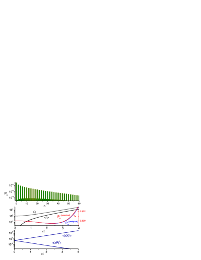
Figure 1: Exact numerical results in the resonant regime and the analytical results for $P_{e}$. The photon number distribution $P_{n}\equiv|\langle n|\psi\rangle|^{2}$ is evaluated for $\varepsilon t=3.9$.

In Fig. 2 we show analogous results for the initial state (5) with $\alpha^{2}=1/2$ in the dispersive regime with parameters $x=0$, $g=5\cdot 10^{-3}$, $\Delta=12g$, and $\varepsilon=3\delta$, comparing numerical and analytical values for the photon number distribution. Again, the coincidence is very good, since the differences are seen only for very low probabilities, less than $10^{-4}$. For other quantities, analytical results are indistinguishable from numerical ones in all plots.

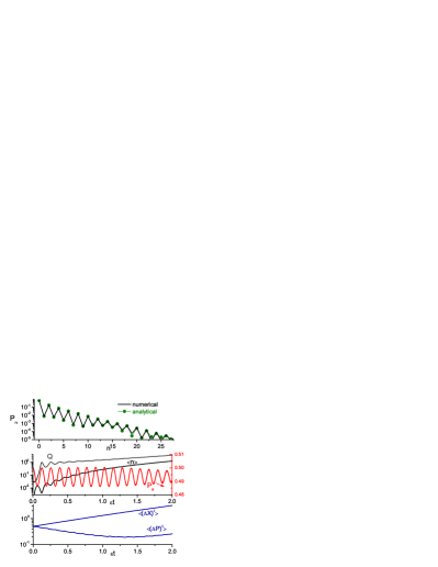
Figure 2: Exact numerical results in the dispersive regime. $P_{n}$ is evaluated for $\varepsilon t=2$, both analytically and numerically.

In conclusion, we obtained closed analytical expressions for the atom-field dynamics generated by the dynamical Casimir effect in the resonant and dispersive regimes, for arbitrary pure atomic initial state. Our results are exact to second order in the small parameters $\zeta=g/\Delta$ and $\xi=2g/\varepsilon$, being in good agreement with numerical data, so they can be used to quantify the influence of the atom on the DCE for different modulation frequencies and atom-cavity detunings. An interesting unsolved problem is to extend the time interval of validity of results from the scales of the order of $\varepsilon^{-1}$ or $g^{-1}$ up to the scales of the order of $\varepsilon^{-2}$ or $g^{-2}$ (in the absence of field-atom coupling some results were obtained in Sriv06 ; Mend11 ).

References

• (1) G. T. Moore, J. Math. Phys. 11, 2679 (1970).
• (2) S. A. Fulling and P. C. W. Davies, Proc. Roy. Soc. London A 348, 393 (1976).
• (3) V. V. Dodonov, Phys. Scr. 82, 038105 (2010).
• (4) D. A. R. Dalvit, P. A. Maia Neto, and F. D. Mazzitelli, in Casimir Physics (Lecture Notes in Physics 834), edited by D. Dalvit, P. Milonni, D. Roberts, and F. da Rosa (Springer, Berlin, 2011), p. 419.
• (5) P. D. Nation, J. R. Johansson, M. P. Blencowe, and F. Nori, Rev. Mod. Phys. (to appear), e-print arXiv: 1103.0835.
• (6) C. M. Wilson, G. Johansson, A. Pourkabirian, M. Simoen, J. R. Johansson, T. Duty, F. Nori, and P. Delsing, Nature 479, 376 (2011).
• (7) G. Barton and C. Eberlein, Ann. Phys. (NY) 227, 222 (1993); P. A. Maia Neto and L. A. S. Machado, Phys. Rev. A 54, 3420 (1996).
• (8) V. V. Dodonov and A. B. Klimov, Phys. Lett. A 167, 309 (1992).
• (9) C. K. Law, Phys. Rev. A 49, 433 (1994).
• (10) V. V. Dodonov and A. B. Klimov, Phys. Rev. A 53, 2664 (1996); G. Plunien, R. Schützhold, and G. Soff, Phys. Rev. Lett. 84, 1882 (2000); M. Crocce, D. A. R. Dalvit, and F. D. Mazzitelli, Phys. Rev. A 64, 013808 (2001).
• (11) C. Braggio, G. Bressi, G. Carugno, C. Del Noce, G. Galeazzi, A. Lombardi, A. Palmieri, G. Ruoso, and D. Zanello, Europhys. Lett. 70, 754 (2005).
• (12) W.-J. Kim, J. H. Brownell, and R. Onofrio, Phys. Rev. Lett. 96, 200402 (2006).
• (13) G. Giunchi, A. Figini Albisetti, C. Braggio, G. Carugno, G. Messineo, G. Ruoso, G. Galeazzi, and F. Della Valle, IEEE Trans. Appl. Supercond. 21, 745 (2011).
• (14) F. X. Dezael and A. Lambrecht, EPL 89, 14001 (2010); D. Faccio and I. Carusotto, EPL 96, 24006 (2011).
• (15) V. V. Dodonov, Phys. Lett. A 207, 126 (1995).
• (16) A. M. Fedotov, N. B. Narozhny, and Y. E. Lozovik, Phys. Lett. A 274, 213 (2000).
• (17) T. Kawakubo and K. Yamamoto, Phys. Rev. A 83, 013819 (2011).
• (18) A. Blais, R.-S. Huang, A. Wallraff, S. M. Girvin, and R. J. Schoelkopf, Phys. Rev. A 69, 062320 (2004); M. Wallquist, K. Hammerer, P. Rabl, M. Lukin, and P. Zoller, Phys. Scr. T137, 014001 (2009); S. M. Girvin, M. H. Devoret, and R. J. Schoelkopf, Phys. Scr. T137, 014012 (2009); A. V. Dodonov, J. Phys.: Conf. Ser. 161, 012029 (2009).
• (19) V.I. Man’ko, J. Sov. Laser Res. 12, 383 (1991); K. Takashima, N. Hatakenaka, S. Kurihara, and A. Zeilinger, J. Phys. A 41, 164036 (2008); A. V. Dodonov, L. C. Céleri, F. Pascoal, M. D. Lukin, and S. F. Yelin, e-print arXiv:0806.4035.
• (20) A. V. Dodonov, R. Lo Nardo, R. Migliore, A. Messina, and V. V. Dodonov, J. Phys. B 44, 225502 (2011).
• (21) A. V. Dodonov and V. V. Dodonov, Phys. Lett. A 375, 4261 (2011).
• (22) E. T. Jaynes and F. W. Cummings, Proc. IEEE 51, 89 (1963); H. Paul, Ann. Phys. (Leipzig) 11, 411 (1963).
• (23) S. De Liberato, D. Gerace, I. Carusotto, and C. Ciuti, Phys. Rev. A 80, 053810 (2009).
• (24) R. R. Puri, Mathematical Methods of Quantum Optics (Springer, Berlin, 2001).
• (25) Y. N. Srivastava, A. Widom, S. Sivasubramanian, and M. Pradeep Ganesh, Phys. Rev. A 74, 032101 (2006).
• (26) J. T. Mendonça, G. Brodin, and M. Marklund, Phys. Lett. A 375, 2665 (2011).