Ejections of magnetic structures above a spherical wedge driven by a convective dynamo with differential rotation

Abstract

We combine a convectively driven dynamo in a spherical shell with a nearly isothermal density-stratified cooling layer that mimics some aspects of a stellar corona to study the emergence and ejections of magnetic field structures. This approach is an extension of earlier models, where forced turbulence simulations were employed to generate magnetic fields. A spherical wedge is used which consists of a convection zone and an extended coronal region to $\approx 1.5$ times the radius of the sphere. The wedge contains a quarter of the azimuthal extent of the sphere and $150\hbox{${}^{\circ}$}$ in latitude. The magnetic field is self-consistently generated by the turbulent motions due to convection beneath the surface. Magnetic fields are found to emerge at the surface and are ejected to the coronal part of the domain. These ejections occur at irregular intervals and are weaker than in earlier work. We tentatively associate these events with coronal mass ejections on the Sun, even though our model of the solar atmosphere is rather simplistic.

1 Introduction

Recent observations of the Solar Dynamics Observatory (SDO: Pesnell, Thompson, and Chamberlin, 2012) have provided us with a record of impressive solar eruptions. These eruptions are mostly associated with coronal mass ejections (CMEs). These are events through which the Sun sheds hot plasma and magnetic fields from the corona into the interplanetary space. The energy causing such huge eruptions is stored in the magnetic field and can be released via reconnection of field lines (Sturrock, 1980; Antiochos, De Vore, and Klimchuk, 1999). Some of the CMEs are directed towards the Earth, hitting its magnetosphere and causing phenomena like aurorae. Furthermore, encounters with CMEs can cause sudden outages of GPS signals due to ionospheric scintillation. The resulting radiation dose from such events poses risks to astronauts. This is now also of concern to airlines, because the radiation load during polar flights can reach annual limits, especially for pregnant women. This leads to great interest of scientists in many fields of physics. However, there is an additional motivation which comes along with space weather effects. The solar dynamo, which is broadly believed to be responsible for the generation of the solar magnetic field, needs to be sustained by shedding magnetic helicity from the Sun’s interior (Blackman and Brandenburg, 2003). Mean-field and direct numerical simulations have shown that the magnetic field generation is catastrophically quenched at high magnetic Reynolds numbers in closed systems (Vainshtein and Cattaneo, 1992) that do not allow magnetic helicity fluxes out of the domain (Blackman and Field, 2000a, b; Brandenburg and Sandin, 2004), or between different parts of it (Brandenburg, Candelaresi, and Chatterjee, 2009; Mitra et al., 2010; Hubbard and Brandenburg, 2010). The magnetic Reynolds number, which quantifies the relative importance of advective to diffusive terms in the induction equation, is known to be very large in the Sun, therefore implying the possibility of catastrophic quenching in models of the solar dynamo, unless efficient magnetic helicity fluxes occur, for example through CMEs (Blackman and Brandenburg, 2003). Indeed, CMEs are well known to be closely associated with magnetic helicity (Low, 2001). In particular observations (Plunkett et al., 2000; Régnier, Amari, and Kersalé, 2002) and a recent study by Thompson, Kliem, and Török (2011), where the observations are compared with numerical models, suggest that CMEs have a twisted magnetic structure, implying that CMEs transport helicity outwards.

There has been significant progress in the study of CMEs in recent years. In addition to improved observations from spacecrafts, e.g. SDO or the Solar TErestical RElation Observatory (STEREO: Kaiser et al., 2008)), there have also been major advances in the field of numerical modeling of CME events (Russev et al., 2003; Archontis et al., 2009). However, the formation and the origin of eruptive events like CMEs is not yet completely understood. Simulating CMEs and their formation is challenging. Leaving the difficulties of modeling the interplanetary space aside, a CME, after being ejected into the chromosphere or the lower corona, travels over an extended radial distance to the upper corona. In this environment, density and temperature vary by several orders of magnitude, which is not easy to handle in numerical models. Additionally, the origin of the CMEs is assumed to relate to the magnetic fields and the velocity pattern at the surface. However, the surface magnetic and velocity fields are rooted in the solar convection zone, where convective motions, in interplay with differential rotation, generate the magnetic field and the velocity patterns that are observed at the surface. The majority of researchers modeling CMEs do not include the convection zone in their setup, and thereby neglect the effect of the magnetic and velocity fields being rooted to this layer. Often the initial conditions for the magnetic and velocity fields are prescribed or taken from 2D observations; see for example Antiochos, De Vore, and Klimchuk (1999) and Amari et al. (1999) as well as Török and Kliem (2003).

Another approach is to study the emergence of flux ropes from the lower convection zone into the corona. In the presence of strong shear, convection simulations have been showing the formation of flux tubes (, 2011; Nelson et al., 2011), but such structures are similar to vortex tubes whose diameter is known to relate with the visco-resistive scale (Brandenburg, Procaccia, and Segel, 1995). In other approaches flux ropes are inserted in a self-consistent model, but their origin is left unexplained. In several recent papers (Martí­nez-Sykora, Hansteen, and Carlsson, 2008; Jouve and Brun, 2009; Fang et al., 2010), the focus lies on the emergence of magnetic flux and the resulting features in the solar atmosphere. However, eruptive events have not been investigated with this setup. In earlier work (Warnecke and Brandenburg, 2010, hereafter WB) a different approach was developed. The solar convection zone was combined with a simple model of the solar corona. The magnetic field, which was here generated by dynamo action beneath the solar surface, emerged through the surface and was ejected out of the domain. The focus was on the connection of the dynamo-generated field and eruptive events like CMEs through the dynamo-generated twist. WB used a simplified coronal model and drove the dynamo with forced turbulence. These simplifications allowed them to study the emergence and a new mechanism to drive ejections in great detail. In subsequent work (Warnecke, Brandenburg, and Mitra, 2011, hereafter WBM), the setup of WB was improved by using a spherical coordinate system and helical forcing with opposite signs in each hemisphere to mimic the effects of rotation on inhomogeneous turbulence. In addition, WBM included the stratification resulting from radial gravity for an isothermal fluid. To improve this model, we now employ convection to generate the velocity field. In a related approach, Pinto and Brun (2011) considered convective overshoot into the chromosphere and the excitation of gravity waves therein, but dynamo-generated twist seemed to be unimportant in their work. The turbulent motions driving the generation of magnetic field are now self-consistently generated by convective cells operating beneath the surface. The setup of the convection zone follows ideas of Käpylä, Korpi, and Brandenburg (2008), Käpylä et al. (2010, 2011) and Käpylä, Mantere, and Brandenburg (2011, 2012). There are other approaches simulating convection in hot massive stars, which have thin subsurface convection zones (Cantiello et al., 2011). But we now use an extended cooling layer to describe some properties of a solar corona. The results of this work complement those of earlier work and can be compared with observations. The model of the solar atmosphere is still a very simplified one, but can be regarded as a preliminary step, which will provide a reference point for improved work in that direction.

2 The model

model As in WB and WBM, a two-layer model is used, which represents the convection zone and an extended corona-like layer in one and the same model. Our convection zone is similar to those of Käpylä et al. (2010, 2011). The domain is a segment of the Sun and is described in spherical polar coordinates $(r,\theta,\phi)$. We model the convection zone starting at radius $r=0.7\,R$ and the solar corona until $r=R_{c}$, where $R_{c}=1.5\,R$ in the present models, where $R$ corresponds to the solar radius. In the latitudinal direction, our domain extends in colatitude from $\theta=15^{\circ}$ to $165^{\circ}$ and in the azimuthal direction from $\phi=0^{\circ}$ to $90^{\circ}$. We solve the following equations of compressible magnetohydrodynamics:

$${\partial\mbox{\boldmath$A$}{}\over\partial t} = \mbox{\boldmath$U$}{}\times\mbox{\boldmath$B$}{}+\eta\mbox{\boldmath$\nabla$}{}^{2}\mbox{\boldmath$A$}{},$$ (1)

$${{\rm D}{}\ln\rho\over{\rm D}{}t} = -\mbox{\boldmath$\nabla$}{}\cdot\mbox{\boldmath$U$}{},$$ (2)

$${{\rm D}{}\mbox{\boldmath$U$}{}\over{\rm D}{}t} = \mbox{\boldmath$g$}{}-2\mbox{\boldmath$\Omega$}{}_{0}\times\mbox{\boldmath$U$}{}+{1\over\rho}\left(\mbox{\boldmath$J$}{}\times\mbox{\boldmath$B$}{}-\mbox{\boldmath$\nabla$}{}p+\mbox{\boldmath$\nabla$}{}\cdot 2\nu\rho\mbox{\boldmath${\sf S}$}{}\right)-\mbox{\boldmath$D$}{}(r,\theta,t),$$ (3)

$$T{{\rm D}{}s\over{\rm D}{}t} = {1\over\rho}\mbox{\boldmath$\nabla$}{}\cdot K\mbox{\boldmath$\nabla$}{}T+2\nu\mbox{\boldmath${\sf S}$}{}^{2}+{\mu_{0}\eta\over\rho}\mbox{\boldmath$J$}{}^{2}-\Gamma_{\rm cool},$$ (4)

where the magnetic field is given by $\mbox{\boldmath$B$}{}=\mbox{\boldmath$\nabla$}{}\times\mbox{\boldmath$A$}{}$ and thus obeys $\mbox{\boldmath$\nabla$}{}\cdot\mbox{\boldmath$B$}{}=0$ at all times, $\mu_{0}$ is the vacuum permeability, $\eta$ and $\nu$ are the magnetic diffusivity and kinematic viscosity, respectively, ${\rm D}{}/{\rm D}{}t=\partial/\partial t+\mbox{\boldmath$U$}{}\cdot\mbox{\boldmath$\nabla$}{}$ is the advective time derivative, $\rho$ is the density, and $U$ is the velocity. The traceless rate-of-strain tensor is given by

$${\mathsf{S}}_{ij}={\textstyle{1\over 2}}(U_{i;j}+U_{j;i})-{\textstyle{1\over 3}}\delta_{ij}\mbox{\boldmath$\nabla$}{}\cdot\mbox{\boldmath$U$}{},$$ (5)

where semicolons denote covariant differentiation; see Mitra et al. (2009) for details. $\mbox{\boldmath$\Omega$}{}_{0}=\Omega_{0}(\cos\theta,-\sin\theta,0)$ is the rotation vector, $p$ is the pressure, $K$ is the radiative heat conductivity, and $\mbox{\boldmath$D$}{}(r,\theta,t)$ describes damping in the coronal region; see Section damp for details. The gravitational acceleration is given by

$$\mbox{\boldmath$g$}{}=-GM\mbox{\boldmath$r$}{}/r^{3},$$ (6)

where $G$ is Newton’s gravitational constant, and $M$ is the mass of the star. The fluid obeys the ideal gas law, $p=(\gamma-1)\rho e$, where $\gamma=c_{p}/c_{v}=5/3$ is the ratio of specific heats at constant pressure and constant volume, respectively, and $e=c_{v}T$ is the internal energy density, which defines the temperature $T$. The cooling term $\Gamma_{\rm cool}$ will be explained in Equation (cool) below in more detail.

2.1 Initial setup and boundary conditions

For the thermal stratification in the convection zone, we consider a simple analytical setup instead of profiles from solar structure models as in, e.g., Brun et al. (2004). The hydrodynamic temperature gradient is given by

$${\partial T\over\partial r}={-|\mbox{\boldmath$g$}{}|\over c_{v}(\gamma-1)(m+1)},\ilabel{gradt}$$ (7)

where $m=m(r)$ is the radially varying polytropic index, for which we assume a stepwise constant profile. We also use Equation (gradt) as the lower boundary condition for the temperature. This gives the logarithmic temperature gradient $\nabla$ (familiar to those working in stellar physics, but not to be confused with the operator $\nabla$) as

$$\nabla={\partial\ln T\over\partial\ln p}={1\over m+1}.$$ (8)

The stratification is convectively unstable if $\nabla-\nabla_{\rm ad}>0$, where $\nabla_{\rm ad}=1-1/\gamma$ is the adiabatic temperature gradient, corresponding to $m<1.5$ for unstable stratification. We choose $m=1$ in the convectively unstable layer beneath the surface, $r<R$. The region above $r=R$ is stably stratified and isothermal due to a cooling term $\Gamma_{\rm cool}$ with respect to a constant reference temperature in the entropy equation. The density stratification is obtained by requiring the hydrostatic equilibrium condition to be satisfied.

Figure 1.: Initial stratification of temperature (dashed line), density (solid), pressure (dot-dashed) and the Brunt–Väisälä frequency $N^{2}=-(|\mbox{\boldmath$g$}{}|/H_{p})(\nabla-\nabla_{\rm ad})$ (dash-triple-dotted) for Run A5. The subscripts $b$ refers to the values at $r=0.7\,R$. The dotted horizontal (vertical) line denotes the value of zero ($r=R$). strat

The thermal conductivity follows from the constancy of the radial luminosity profile $L(r)=L_{0}={\rm const}{}$ throughout the domain and is given by

$$K={L_{0}\over 4\pi r^{2}\partial T/\partial r}.$$ (9)

To speed up the thermal relaxation processes, we apply shallower profiles, corresponding to $\rho\propto T^{1.4}$, for the thermal variables within the convectively unstable layer. The value $m=1$ is just used in the convection zone to determine the thermal conductivity. In Figure strat we show the initial non-convecting stratification. The radial temperature gradient at the bottom of the domain is set to a constant value, which leads to a constant heat flux into the domain. In the coronal part the gradient goes smoothly to $0$ by using the $r$ dependent cooling function $\Gamma_{\rm cool}$, which is included in the entropy evolution (entro). The cooling term is given by

$$\Gamma_{\rm cool}=\Gamma_{0}f(r)\left({c_{\rm s}^{2}-c^{2}_{s0}\over c^{2}_{s0}}\right),\ilabel{cool}$$ (10)

where $f(r)$ is a profile function equal to unity in $r>R$ and smoothly connecting to zero in $r\leq R$, and $\Gamma_{0}$ is a cooling luminosity chosen so that the sound speed in the coronal part relaxes towards $c^{2}_{\rm s0}\equiv c_{\rm s}^{2}(r=R_{c})$. Whether the stratification is convectively stable or not depends on the Brunt–Väisälä frequency $N$, defined through

$$N^{2}=|\mbox{\boldmath$g$}{}|\left({1\over\gamma}{\partial\ln p\over\partial r}-{\partial\ln\rho\over\partial r}\right)=-{|\mbox{\boldmath$g$}{}|\over H_{p}}\left(\nabla-\nabla_{\rm ad}\right),$$ (11)

where $H_{p}=-\partial r/\partial\ln p$ is the pressure scale height. If $N^{2}$ is negative, the stratification is unstable.

We initialize the magnetic field as a weak, random, Gaussian-distributed seed field in the whole domain. In the coronal part the magnetic field diffuses after a short time. We do not use a background coronal field, so the field is self-consistently generated by the dynamo in the convective layer. We apply periodic boundary conditions in the azimuthal direction over a $90^{\circ}$ fraction of the full circumference. For the velocity we take stress-free boundary conditions on all other boundaries. As in WBM, the stress-free boundary conditions prevent mass flux, so no stellar wind is possible. Because no mass can escape, material will eventually fall back from the boundary. Thermodynamic variables have zero gradients at the latitudinal boundaries. We employ perfect conductor boundaries for the magnetic field at the latitudinal and at the lower radial boundaries, and radial field conditions at the outer radial boundary. The latter is motivated by the fact that in the Sun, the solar wind pushes the magnetic field to open field lines and at a radius of $r=2.0\ldots 2.5$ solar radii. the field lines are mostly radial (Levine, Schulz, and Frazier, 1982; , 1982). This choice has been substantiated by subsequent work of Wang and Sheeley (1992) as well as Schrijver and De Rosa (2003). While this choice might still be too restrictive for coronal holes and coronal streamers, and given also that our radial extent in most of the simulations is smaller than $r=2R$, we nevertheless choose the vertical field boundary condition because it satisfies our primary objective of letting magnetic helicity leave the domain, which is believed to be crucial for the dynamo to operate at large values of $\mbox{\rm Re}_{M}$ (Blackman and Field, 2000a, b; Brandenburg and Sandin, 2004). However, we must be aware of the fact that with this choice our description of the field in the exterior layer is not a realistic one.

To describe the corona as an isothermal extended cooling layer is a serious simplification, in that the temperature inside the coronal layer is not higher than in the convection zone as in a real stellar corona, but it stays fixed at the surface value; see Figure strat. Besides the fact that a simple cooling layer is easy to handle numerically, we emphasize the importance of facilitating comparison with previous models of WBM. It can also be seen as a step towards studying effects that are not solely due to a low plasma $\beta$ corona, for which the magnetic pressure, i.e. the magnetic field, is strong compared with the gas pressure ($\beta=2\mu_{0}p/\mbox{\boldmath$B$}{}^{2}$). Indeed, given that our initial field is weak, the plasma $\beta$ is necessarily large in the outer parts. We note that it is not even clear whether a hot corona promotes or hinders coronal ejections. To understand the formation and evolution of magnetic ejections, studies that isolate these effects, such as the present one, may be important.

We use the Pencil Code with sixth-order centered finite differences in space and a third-order accurate Runge–Kutta scheme in time; see Mitra et al. (2009) for the extension of the Pencil Code to spherical coordinates. We use a grid size of $128\times 128\times 64$ mesh points (Runs A5 and Ar1), and $256\times 256\times 128$ (Run A5a).

2.2 Velocity damping in the corona

damp

Whether the solar corona rotates like a solid body or differentially coupled with the photosphere is unclear. In recent work by Wöhl et al. (2010), where SOHO-EIT data of the bright points in the solar corona were used to estimate the rotation speeds, it was found that the corona rotates similarly as the small magnetic features in the photosphere. Similar results have been obtained by Badalyan (2010), where the coronal rotation has been measured by analyzing the green Fe^XIV 530.3 nm line. This author finds also a variation pattern with the activity cycle. However, the observations of the “boot” coronal hole by SKYLAB suggested rigid rotation (Timothy et al., 1975). Recent work on coronal holes by Lionello et al. (2005) claims that the rigid rotation is only an apparent one. The magnetic field is sheared by the differential rotation, but the boundary of the hole remains relatively unchanged, due to reconnection. Owing to the low plasma $\beta$ in the solar corona, the fluid motions are dominated by the magnetic fields whose footpoints are anchored in the photosphere or even further down. So the magnetic field might then be rigid enough to prevent differential rotation of the solar corona. However, the observed bright points and other features in the corona are strongly correlated with the magnetic field so they can give a misleading picture about the global rotation of the corona.

In our simulations, the Coriolis force is included in the momentum equation as a consequence of the rotation. In the solar corona the density is more than 14 orders of magnitude smaller than in the lower convection zone. Because of the weak density stratification in our simulation, the Coriolis force in our coronal part is too strong and can cause possible artifacts such as the magnetorotational instability. To avoid this—at least for runs with rapid rotation—we apply a damping function $\mbox{\boldmath$D$}{}(r,\theta)$ in the momentum equation, which is given by

$$\mbox{\boldmath$D$}{}(r,\theta,t)={1\over\tau_{\rm D}}\Theta(r-R)\,\overline{\mbox{\boldmath$U$}{}}(r,\theta,t),$$ (12)

where

$$\Theta(r-R)={\textstyle{1\over 2}}\left[1+\tanh{\left({r-R\over w}\right)}\right],$$ (13)

with $\tau_{\rm D}$ being the damping time and $w$ the width of the transition layer from convection zone to the coronal part. Here and elsewhere, the overbar denotes averaging over $\phi$, defined as $\overline{F}(r,\theta,t)$=$\int{F(r,\theta,\phi,t)\;{\rm d}{}\phi/2\pi}$. Occasionally we also use time averages denoted by $\langle.\rangle_{t}$.

2.3 Units, nondimensional quantities, and parameters

nond

Dimensionless quantities are obtained by setting

$$R=GM=\rho_{\rm b}=c_{p}=\mu_{0}=1,$$ (14)

where $\rho_{\rm b}$ is the density at $r=0.7\,R$. Below, we will describe the properties of the runs by the following dimensionless parameters: fluid Reynolds number $\mbox{\rm Re}=u_{\rm rms}/\nu k_{\rm f}$, magnetic Reynolds number $\mbox{\rm Re}_{M}=u_{\rm rms}/\eta k_{\rm f}$, where $k_{\rm f}=2\pi/0.3R$ is an estimate for the typical wavenumber of the energy-carrying eddies and $u_{\rm rms}=\sqrt{3/2\langle U_{r}^{2}+U_{\theta}^{2}\rangle}$ is the volume-averaged rms velocity in the convection zone ($r\leq R$). In our definition of $u_{\rm rms}$ we omit the contribution from the $\phi$-component of the velocity, because it is dominated by contributions from the large-scale differential rotation that develops when rotation is included and would give an atypical estimate of the convective turnover time. To compensate for this, and to have an estimate of $u_{\rm rms}$ comparable with earlier work, we apply the 3/2 correction factor. We also define the magnetic Prandtl number $\mbox{\rm Pr}_{M}=\nu/\eta=\mbox{\rm Re}_{M}/\mbox{\rm Re}$ and the Coriolis number $\mbox{\rm Co}=2\Omega_{0}/u_{\rm rms}k_{\rm f}$. Time is expressed in units of $\tau=\left(u_{\rm rms}k_{\rm f}\right)^{-1}$, which is the eddy turnover time in the convection zone. We measure the magnetic field strength as the rms value averaged over the convection zone $B_{\rm rms}$, where we often normalize this value with the equipartition value of the magnetic field defined by $B_{\rm eq}^{2}=\mu_{0}\langle\overline{\rho}u_{\rm rms}^{2})\rangle_{r\leq R}$. The relative kinetic helicity is $h_{\rm rel}(r,t)=\overline{\mbox{\boldmath$\omega$}{}\cdot\mbox{\boldmath$u$}{}}/\omega_{\rm rms}u_{\rm rms}$, where $\mbox{\boldmath$\omega$}{}=\mbox{\boldmath$\nabla$}{}\times\mbox{\boldmath$u$}{}$ is the vorticity and $\omega_{\rm rms}$ is its rms value inside the convection zone.

3 Results

results

Table 1.: Summary of the runs. Re is the fluid Reynolds number, $u_{\rm rms}=\sqrt{3/2(U_{r}^{2}+U_{\theta}^{2})}$ is the volume-averaged rms velocity in the convection zone normalized by $\sqrt{GM/R}$, $\mbox{\rm Pr}_{M}$ is the magnetic Prandtl number, Co is the Coriolis number, and $h_{\rm rel}$ is the maximum value of the relative kinetic helicity using azimuthal averages as defined in Section nond. $\rho_{\rm b}\over\rho_{\rm s}$ and $\rho_{\rm b}\over\rho_{\rm t}$ give the density ratios of the bottom of the convection zone to those at the surface and the top of the domain, respectively. In the right-most column we note if damping for velocity in the coronal part is used (Y) or not (N); see Section damp. summary

Run	Resolution	$\displaystyle{u_{\rm rms}\over\sqrt{GM/R}}$	Re	$\mbox{\rm Pr}_{M}$	$\displaystyle{B_{\rm rms}^{2}\over B_{\rm eq}^{2}}$	$\displaystyle{\rho_{\rm b}\over\rho_{\rm s}}$	$\displaystyle{\rho_{\rm b}\over\rho_{\rm t}}$	Co	$h_{\rm rel}$	$D$
A5	$128^{2}\times 64$	0.0072	3.3	10	0.1–0.4	3.6	39	7	0.5	N
A5a	$256^{2}\times 128$	0.0105	100	1	0.2	3.6	39	4.5	0.3	N
Ar1	$128^{2}\times 64$	0.0040	38	1	1.5–5.5	3.6	39	50	0.3	Y

3.1 Hydrodynamic phase of the simulations

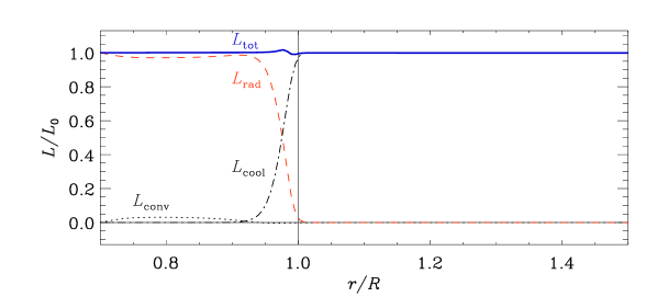
Figure 2.: Flux balance from Run A5. The different contributions to the total luminosity (solid blue line) are due to radiative diffusion (dashed red line), resolved convection (dotted black line) and cooling (dash-triple-dotted black line). The black thin line denotes the zero level and the surface ($r=R$), respectively. pflux

After around 100 turnover times, convection has reached saturation and we find convection cells as typical patterns in the radial velocity just below the surface. In our model, the dominant energy transport mechanisms are radiative and convective fluxes in the bulk of the convection zone and an (optically thin) cooling flux in the outer (coronal) parts. The radiative and convective fluxes are defined as:

$$F_{\rm rad}=-K{\partial\overline{T}\over\partial r},\quad F_{\rm conv}=c_{P}\overline{\rho}\overline{u_{r}^{\prime}T^{\prime}},$$ (15)

where the averages are taken over $\theta$ and $\phi$ and the prime indicates fluctuations about the respective mean quantity. In our present setup, however, the convective flux reaches barely about 5% in the convection zone; see Figure pflux where we plot the relevant contributions to the luminosity for Run A5. Above the surface the cooling takes over to maintain an approximately isothermal atmosphere. The total flux is constant, except for small departures near the surface. The kinetic energy and viscous fluxes are negligible in the present runs.

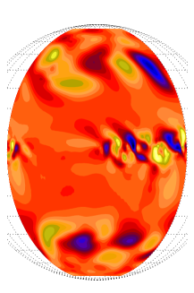
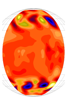
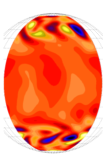
Figure 3.: Radial velocity ($U_{r}$) above the surface for $r=1.15$, 1.25, $1.35\,R$ from left to right, for Run A5. Dark blue shades represent negative and light yellow positive values. urad2

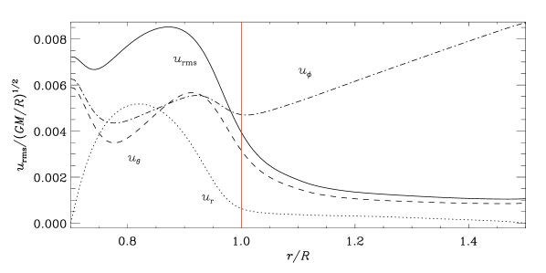
Figure 4.: Root-mean-square values of $U_{r}$ (dotted), $U_{\theta}$ (dashed), and $U_{\phi}$ (dash-dotted) as a function of radius for Run A5. The solid line shows the radial profile of our nominal rms velocity, $u_{\rm rms}=\sqrt{3/2(U_{r}^{2}+U_{\theta}^{2})}$. The (red) vertical line indicated the surface at ($r=R$). The values are normalized by $\sqrt{GM/R}$. urms

To determine the degree of overshooting and penetration into the stably stratified layers above the convection zone, we show in Figure urad2 the radial velocity above the surface at $r=1.15$, $1.25$, and $1.35\,R$ for Run A5. At low latitudes, there is very little radial penetration (velocity features are only seen until $r=1.15\,R$), while at higher latitudes the radial velocity pattern is transmitted all the way to $1.35\,R$. This is not surprising in view of the Taylor–Proudman theorem, which states that for rapid rotation (large values of Co) the local angular velocity of the gas is constant along cylindrical surfaces.

Next, we plot in Figure urms the rms values of all three velocity components for Run A5. The amplitude of the radial velocity component falls off the fastest. The latitudinal component also falls off with radius, but remains about three times larger than the radial component. The longitudinal component, on the other hand, increases with radius in a way that is compatible with rigid rotation with an angular velocity that is somewhat larger than the rotation rate of the frame of reference.

The size of the convection cells depends strongly on the strength of rotation and the degree of density stratification; see also Käpylä, Mantere, and Brandenburg (2011). We plot the radial velocity $U_{r}$ at $r=0.89\,R$ for Runs A5, A5a, and Ar1 in Figure urad. The Run A5 has a low fluid Reynolds number and therefore the convection cells are large; see Table summary. The flow pattern shows clear ‘banana cells’ as in previous work with comparable Coriolis parameter, cf. Käpylä et al. (2011). A higher fluid Reynolds number and higher resolution, as in Run A5a, allow the velocity field to form more complex structures. However, the banana cells are still visible. If one now looks at a simulation with more rapid rotation (Run Ar1, plotted in the right-most panel of Figure urad) with a Coriolis number of $\mbox{\rm Co}=50$, the number of banana cells increases and they are more clearly visible than in Run A5a. Note also that the radial velocity is now significantly reduced at high latitudes inside the inner tangent cylinder.

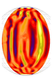
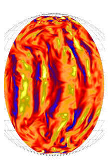
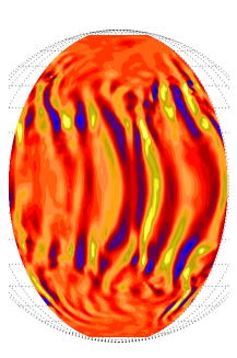
Figure 5.: Radial velocity ($U_{r}$) beneath the surface ($r=0.89\,R$) for Runs A5, A5a, and Ar1 from left to right. Dark blue shades represent negative and light yellow positive values. urad

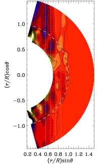
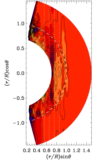
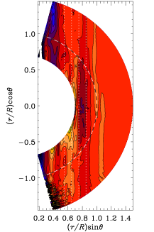
Figure 6.: Differential rotation profiles $\overline{\Omega}(r,\theta)=\overline{U}_{\phi}/(r\sin{\theta})+\Omega_{0}$ for Runs A5, A5a, and Ar1 from left to right. Dark blue shades represent low and light yellow high values, overplotted by the isocontours with solid black lines. The dotted white lines parallel to the rotation axis are given for orientation and the dashed line indicates the surface ($r=R$). difrot

In the Sun, differential rotation is an important element to produce the magnetic field structures observed at large scales, exhibiting a cyclic behavior over time, as manifested by the sunspot cycle. To illustrate the differential rotation profiles generated in the simulations, we plot the azimuthally averaged angular velocity, $\overline{\Omega}(r,\theta)=\overline{U}_{\phi}/(r\sin{\theta})+\Omega_{0}$, for Runs A5, A5a, and Ar1 in the saturated state of the simulation; see Figure difrot. In the plot, we show isocontours of angular velocity with solid black lines. In the convection zone the contours of local angular velocity tend to be cylindrical, which is likely a consequence of the absence of a strong latitudinal modulations of specific entropy (Brandenburg, Moss, and Tuominen, 1992; Kitchatinov and Rüdiger, 1995; Miesch, Brun, and Toomre, 2006). The coronal part seems to rotate as a solid body outside the outer tangent cylinder (i.e., for $r\sin\theta>R$), while inside it some differential rotation occurs also in the coronal part. In the convection zone between the inner and outer tangent cylinders, the angular velocity is enhanced relative to that inside the inner tangent cylinder (see the first and second panels of Figure difrot), while in the case of extremely rapid rotation this may actually be reversed.

In the three runs shown in Figure difrot the stratification in the whole domain is just ${\rho_{\rm b}/\rho_{\rm t}}=40$, which is rather small compared to the stratification of the Sun (${\rho_{\rm b}/\rho_{\rm t}}\sim 10^{14}$). It seems, therefore, that the Coriolis force is acting much more strongly in the coronal part of our simulation than in reality. In the Sun the Lorentz force plays a more important role in the corona than in our model. In the convection zone, we find quenching of convection due to rapid rotation. In Run A5, where $\mbox{\rm Co}=7$, the lines of constant rotation rate are more radial than vertical and show super-rotation, i.e., the equator rotates faster than the poles. As expected, this tends to coincide with locations where the Reynolds stress in the radial direction is negative (see, e.g., Rüdiger, 1980). However, the convection cells are rather big and have a strong local influence on $U_{\phi}$ and could in principle lead to subrotation; see the corresponding discussion in Dobler, Stix, and Brandenburg (2006). Note that the rms velocity in Run A5 is two times smaller than in Run A5a, which has higher resolution and higher fluid and magnetic Reynolds numbers ($\mbox{\rm Re}=\mbox{\rm Re}_{M}=100$). Due to this, we find clear super-rotation, even though the Coriolis number is slightly lower ($\mbox{\rm Co}=4.5$) than what is realized in Run A5. In the third case, Run Ar1, where the rotation is extremely rapid ($\mbox{\rm Co}=50$), we also find super-rotation, where the lines of constant rotation rate are almost all vertical. In comparable work (Käpylä et al., 2011; Käpylä, Mantere, and Brandenburg, 2011), super-rotation has been found, when the Coriolis number was larger than 4. This is similar to our results including a coronal part. In addition, there is a minimum of the rotation rate at mid-latitudes and a polar vortex at high latitudes. Rotation profiles, which show a comparable behavior, have been found by several groups (Miesch et al., 2000; Elliot, Miesch, and Toomre, 2000; Käpylä et al., 2011; Käpylä, Mantere, and Brandenburg, 2011). The region with the higher rotation rate near the equator is limited to the upper convection zone and can even penetrate into the coronal part. In Run Ar1 the velocity damping described in Section damp is used. By comparing the right-most panel of Figure difrot, with damping, to the left-most panels, without it, we conclude that the damping does not make much of a difference to the coronal velocity structures.

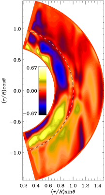
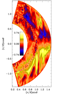
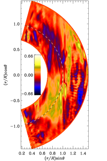
Figure 7.: Relative helicity $h_{\rm rel}(r,t)=\overline{\mbox{\boldmath$\omega$}{}\cdot\mbox{\boldmath$u$}{}}/\omega_{\rm rms}u_{\rm rms}$ plotted for Runs A5, A5a, and Ar1 from left to right. Dark blue shades represent negative and light yellow positive values. The dashed line indicates the surface ($r=R$). relhel

Simulations with randomly forced turbulence (WB,WBM) have shown that the relative kinetic helicity $h_{\rm rel}$ has a strong influence both on the generation of large-scale magnetic fields and the ejection events. In WB and WBM, values of $h_{\rm rel}$ of order unity were achieved by using a forcing function with purely helical plane waves. In the convection runs presented here, however, values of large relative helicity, $h_{\rm rel}=0.5$, are obtained (for Run A5), at least at certain radii. In Figure relhel, we present contour plots of azimuthally averaged relative helicity in the meridional plane for Runs A5, A5a, and Ar1. All three show the typical sign rule of kinetic helicity under the influence of rotation, i.e. the northern hemisphere has predominantly a negative sign and the southern a positive one. Close to the bottom of the convection zone, the sign changes, which has earlier been reported by several authors both in Cartesian (e.g. Brandenburg et al., 1990; Ossendrijver, Stix, and Brandenburg, 2001) and spherical geometries (e.g. Miesch et al., 2000; Käpylä et al., 2010). Only in Run Ar1 with rapid rotation, the behavior is not that clear. The relative helicity is no longer confined to the convection zone, but significant values occur also in the coronal region. The sign rule still holds within the convection zone, while a more complicated sign behavior is visible in the coronal part. The maximal values of the azimuthally averaged helicity are around $h_{\rm rel}=0.3$, occurring close to the surface. In Run A5a, the maximum value is slightly higher and is located in the middle of the convection zone, although relatively high values are present in the coronal part as well. It is not yet completely clear how high values of relative kinetic helicity can be achieved; strong rotation tends to suppress it, whereas strong stratification increases it. Its exact role in generating coronal ejections is yet unclear.

3.2 Convective dynamo

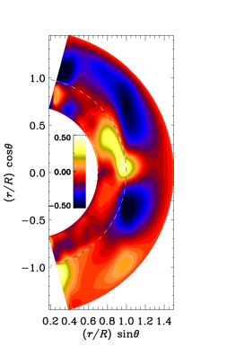
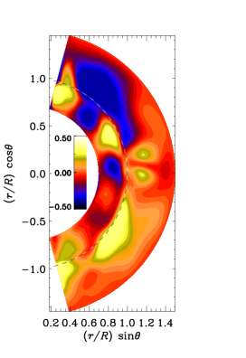
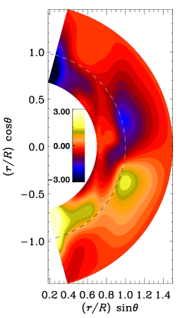
Figure 8.: Time-averaged $\overline{B}_{\phi}$ for Run A5, Ar5a, and Ar1 from left to right. Dark blue shades represent negative and light yellow positive values. The magnetic field is normalized by the equipartition value. The dashed line indicates the surface ($r=R$). bphi

The convective motions generate a large-scale magnetic field due to dynamo action. The magnetic field grows first exponentially and begins then to affect the velocity field. The effects of this backreaction can be subtle in that we found a 6% enhancement of the rms velocity after saturation. The growth of the magnetic field saturates after around 200 to 1000 turnover times, depending on the Coriolis and Reynolds numbers. In the runs in Table summary, we obtain different dynamo solutions for the saturated field.

In Figure bphi we show the time-averaged azimuthal magnetic field $\overline{B}_{\phi}$ for Run A5, A5a, and Ar1. Note that the $\phi$ component of the magnetic field is also strong in the coronal part and roughly antisymmetric about the equator. Furthermore we find an oscillation of the volume-averaged rms magnetic field in the convection zone; see the left-hand panel of Figure bu for Run A5. The growth tends to be steeper than the decline, the period being around $t/\tau=220$. The field reaches a maximum of 60% of the equipartition field strength, $B_{\rm eq}$, which is comparable to the values obtained in the forced turbulence counterparts both in Cartesian and spherical coordinates (WB,WBM). Comparing this with the change of the kinetic energy, plotted as fluctuations of the rms velocity squared, we find an anti-correlation with respect to the magnetic field oscillation. The magnetic field is high (low), when the velocity is low (high). In the work by Brun, Browning, and Toomre (2005), the authors interpret this behavior as the interplay of the magnetic backreaction and the dynamo effect of the differential rotation. Due to the Lorentz force a higher magnetic field strength leads to quenching of the differential rotation. An increased magnetic field quenches the Reynolds stress and thus lowers the differential rotation, which limits the magnetic field. A weak magnetic field leads to stronger differential rotation. Similar behavior has been observed also in previous forcing simulations (WBM). This behavior is not seen as clearly in the large-scale magnetic field which shows variations in strength, but not in sign. As shown in Figure but1 for Run A5, the $\overline{B}_{\phi}$ and $\overline{B}_{r}$ have local maxima in time and in latitude, but the overall structure is nearly constant in time. Even though the large-scale field structure is stationary, the small-scale structures show an equatorward migration near the equator. The reason for this is unclear, but meridional circulation does not seem to play a role here.

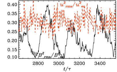
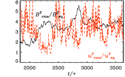
Figure 9.: Phase relation of the magnetic field ($B_{\rm rms}^{2}/B_{\rm eq}^{2}$, solid black lines) and the velocity field ($u_{\rm rms}(t)^{2}/\langle u_{\rm rms}^{2}\rangle_{t}$, dashed red lines) in the convection zone for Runs A5 (left panel) and Ar1 (right). The velocity has been multiplied by a factor of 0.3 (left panel) and 3 (right), respectively, and smoothed over five neighboring data points. bu

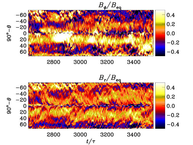
Figure 10.: Variation of $\overline{B}_{\phi}$ and $\overline{B}_{r}$ in the convection zone at $r=0.9R$ for Run A5. Dark blue shades represent negative and light yellow positive values. The dashed horizontal lines show the location of the equator at $\theta=\pi/2$. The magnetic field is normalized by the equipartition value. but1

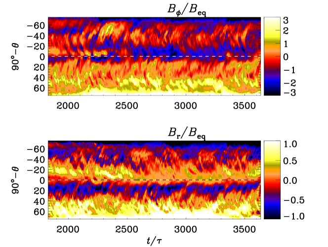
Figure 11.: Variation of $\overline{B}_{\phi}$ and $\overline{B}_{r}$ in the convection zone at $r=0.9R$ for Run Ar1. Dark blue shades represent negative and light yellow positive values. The dashed horizontal lines show the location of the equator at $\theta=\pi/2$. The magnetic field is normalized by the equipartition value. but2

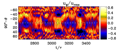
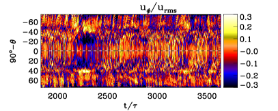
Figure 12.: Variation of $\overline{U}_{\phi}$ in the convection zone at $r=0.9R$ for Run A5 (left panel) and Run Ar1 (right panel). Dark blue shades represent negative and light yellow positive values. The dashed horizontal lines show the location of the equator at $\theta=\pi/2$. The velocity is normalized by the mean rms velocity in the convection zone. uphi

In Run Ar1, the magnetic field reaches up to 5.5 times the equipartition value, but does not show a periodic oscillation; see the right hand panel of Figure bu. In comparable work (Käpylä et al., 2010), similar values for the field strength were found. However, the rms velocity is also quenched, when the magnetic field is high. Looking at $\overline{B}_{\phi}$ and $\overline{B}_{r}$, plotted over time and latitude in Figure but2, the large-scale magnetic field is similar to Run A5, which is constant in time without any oscillation. In the recent work by Käpylä, Mantere, and Brandenburg (2012), the authors found an oscillatory behavior of $\overline{B}_{\phi}$ and $\overline{B}_{r}$ including equatorward migration for latitudes below $60^{\circ}$, which is the first time that such a result is obtained from direct numerical convection simulation of rotating convection.

The azimuthal velocity $\overline{U}_{\phi}$ versus time and latitude (Figure uphi) shows minima at the same times as the maxima of the magnetic field occur. In Run A5a, the occurrence of strong magnetic fields suppresses the differential rotation. The pattern of the azimuthal velocity is symmetric about the equator and shows an oscillatory behavior, which is not that clear in the large-scale magnetic field. In the $\overline{U}_{\phi}$ plot in Figure uphi of Run Ar1, we find just one localized minimum, which coincides with the low values of $u_{\rm rms}(t)^{2}/\langle u_{\rm rms}^{2}\rangle_{t}$ between $t/\tau=2100$ and $2400$.

3.3 Coronal ejections

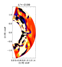
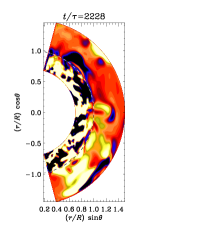
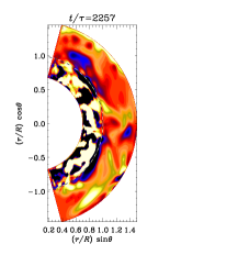
Figure 13.: Time series of a coronal ejection near the equator ($\theta=\pi/2$), taken from Run A5. The normalized current helicity, $\mu_{0}R\,\overline{\mbox{\boldmath$J$}{}\cdot\mbox{\boldmath$B$}{}}/\langle\overline{\mbox{\boldmath$B$}{}^{2}}\rangle_{t}$, is shown in a color-scale representation from different times; dark blue represents negative and light yellow positive values. The dashed horizontal lines show the location of the surface at $r=R$. jb

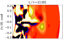
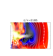
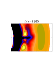
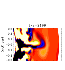
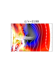
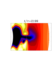
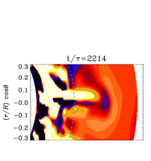
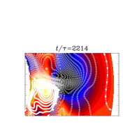
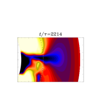
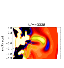
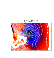
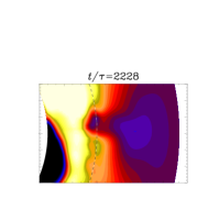
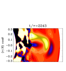
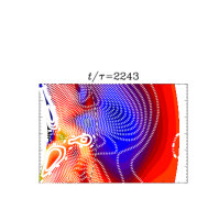
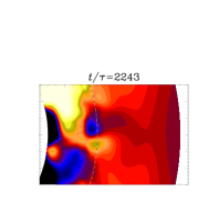
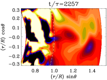
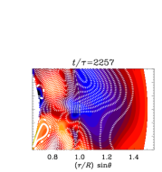
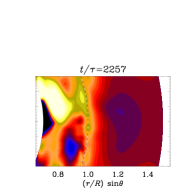
Figure 14.: Time series of a coronal ejection zoomed into the region of the ejection near the equator ($\theta=\pi/2$), taken from Run A5. The dashed horizontal lines show the location of the surface at $r=R$. Left column: normalized current helicity, $\mu_{0}R\,\overline{\mbox{\boldmath$J$}{}\cdot\mbox{\boldmath$B$}{}}/\langle\overline{\mbox{\boldmath$B$}{}^{2}}\rangle_{t}$. Middle column: magnetic field, contours of $r\sin{\theta}\overline{A}_{\phi}$ are shown together with a color-scale representation of $\overline{B}_{\phi}$. The contours of $r\sin{\theta}\overline{A}_{\phi}$ correspond to field lines of $\overline{\mbox{\boldmath$B$}{}}$ in the $r$,$\theta$ plane, where solid lines represent clockwise magnetic field lines and the dashed ones counter-clockwise. Right column: density fluctuations $\Delta\overline{\rho(t)}=\overline{\rho(t)}-\langle\overline{\rho}\rangle_{t}$. For all plots, the color-scale represents negative as dark blue and positive as light yellow. eje

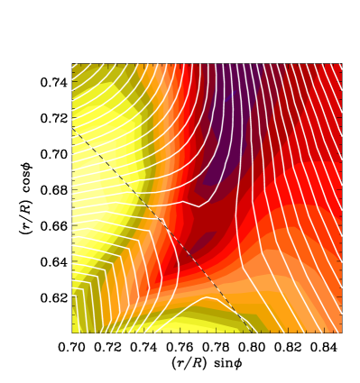
Figure 15.: X-point-like structure in the $r$,$\phi$ plane at the equator ($\theta=\pi/2$) at $t/\tau$=2204 zoomed into the ejection region, taken from Run A5. Contours of $rA_{\theta}$ are shown together with a color-scale representation of $B_{\theta}$; dark blue stands for negative and light yellow for positive values. The contours of $rA_{\theta}$ correspond to field lines of $B$ in the $r$,$\phi$ plane. The dashed horizontal lines show the location of the surface at $r=R$. eje˙phi

In the runs that we have been performed so far, and of which only three have been discussed in this paper, only a small fraction of events can be identified with actual coronal ejections similar to the ones seen in WB and WBM. Especially the Runs A5 and Ar1 show some clear ejection events. There the magnetic field emerges out of the convection zone and is ejected as an isolated structure. In Figure jb we have plotted the normalized current helicity, $\mu_{0}R\,\overline{\mbox{\boldmath$J$}{}\cdot\mbox{\boldmath$B$}{}}/\langle\overline{\mbox{\boldmath$B$}{}^{2}}\rangle_{t}$, as a time series for Run A5. At small scales, the current helicity density, $\mbox{\boldmath$J$}{}\cdot\mbox{\boldmath$B$}{}$, is a good proxy for magnetic helicity density, $\mbox{\boldmath$A$}{}\cdot\mbox{\boldmath$B$}{}$, and is, as opposed to the latter, gauge invariant. In addition, the current helicity can be an indicator of helical magnetic structures, which are believed to be present in coronal mass ejections (Low, 1994, 2001; Plunkett et al., 2000; Régnier, Amari, and Kersalé, 2002; Thompson, Kliem, and Török, 2011). Close to the equator a bipolar structure emerges through the surface. The inner bulk has a positive current helicity, in Figure jb represented by a yellow color, and it pushes an arc with negative current helicity ahead of it; see Figure eje. Such bipolar ejections have been identified in earlier work (WBM) and compared with the ‘three-part structure’ of coronal mass ejection, which is described in Low (1996). The three parts consist of a prominence, which is similar to the bulk seen in our simulations, a front with an arc shaped structure corresponding to our arc, and a cavity between these two features. A bipolarity of twisted magnetic field has also been seen in observed magnetic clouds by Li et al. (1982). Even though the domain of the simulation is larger in the $\theta$ direction than in WBM, the ejections are much smaller, which is actually closer to the CMEs observed on the Sun. In the work of WBM the ejections have a size that corresponds to about 500 Mm, whereas in this work they seems to have a size corresponding to around 100 Mm if scaled to the solar radius. The ejections seem to expand slightly, but no significant expansion rate can be measured using this resolution. Comparing with the forced turbulence runs, the difference in size is mostly due to the more complex and fluctuating magnetic field in convection runs. In the sequence of images of Figure eje, an ejection near the equator reaches the outer boundary and leaves the domain. To investigate the mechanism driving the ejection, we look at the dynamics of the magnetic field in Figure eje, where field lines of the azimuthally averaged mean field are shown as contours of $r\sin{\theta}\overline{A}_{\phi}$, and colors represent $\overline{B}_{\phi}$ together with the density fluctuations and current helicity. During the ejection, one may notice a strong concentration of magnetic field lines that are directed radially outwards. This concentration appears first beneath the surface and then emerges below the current helicity structure and follows it up into the coronal part. Investigating the direction of field lines of the mean field in the time series in Figure eje, an X-point can be found. In the first panel, at $r=1.07\,R$ and $\theta=\pi/2+0.1$, the magnetic field lines form a junction-like shape. The dotted line represents a counter-clockwise oriented field loop, so at the two corners of the junction there are field lines with opposite signs. After around 14 turnover times this “junction” has reconnected at the same position as where the ejection is detected. It appears that these two events are related to each other. Looking at the magnetic field line in the $r$,$\phi$ plane, which here is not averaged over the perpendicular direction (Figure eje_phi), we identify a structure which has a shape similar to an X-point.

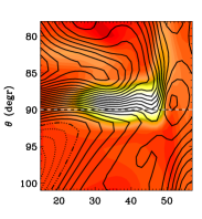
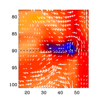
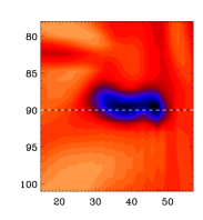
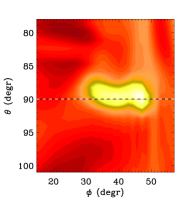
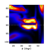
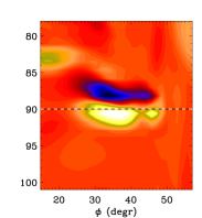
Figure 16.: Different properties of the ejection in the $\theta$,$\phi$ plane at the surface ($r=R$) at $t/\tau=2204$, taken from Run A5. Upper row, left panel: Contours of $A_{r}$ are shown together with a color-scale representation of $B_{r}$; dark blue stands for negative and light yellow for positive values. The contours of $A_{r}$ correspond to field lines of that part of $B$ that is solenoidal in the $\theta$,$\phi$ plane. Solid lines represent clockwise oriented magnetic field lines and dotted lines counter-clockwise ones. Middle panel: The arrows show $(U_{\theta},U_{\phi})$ and colors show $U_{r}$ (blue corresponds to downflows). Right panel: Color-scale representation of the density $\rho$; dark blue stands for low and light yellow for high values. Lower row, left panel: Color-scale representation of specific entropy $s$; dark blue stands for low and light yellow for high values. Middle panel: Color-scale representation of the current density squared $\mbox{\boldmath$J$}{}^{2}$; dark blue stands for low and light yellow for high values. Right panel: current helicity $\mbox{\boldmath$J$}{}\cdot\mbox{\boldmath$B$}{}$, color-scale as in Figure jb. The dashed line indicates the equator at $\theta=\pi/2=90^{\circ}$. eje˙pt

The ejection causes also a strong variation in the density. If the time-averaged density profile is subtracted from instantaneous ones, the density fluctuations are obtained. After removing the density stratification one obtains $\Delta\overline{\rho(t)}=\overline{\rho(t)}-\langle\overline{\rho}\rangle_{t}$. We plot these density fluctuations, $\Delta\overline{\rho(t)}$, in the right column of Figure eje to visualize the effect of the ejection on the density. The density in the ejection is much lower than in the rest of the coronal part. However, the density variations are also associated with fluctuations in the specific entropy ($\Delta s/c_{\rm p}\approx 0.01$), which suggests that thermal buoyancy also plays a role. One interpretation could be that the strong magnetic field reduces the density to achieve total pressure equilibrium and the ejection rises partly because of magnetic buoyancy. Such an effect is also seen by inspecting other ejections.

To characterize the emergence we plot different properties of the ejection in the $\theta$,$\phi$ plane; see Figure eje_pt. The magnetic field shows a strong concentration in its radial and azimuthal components. The concentration is associated with a downflow in spite of it being a low-density region. It is interesting to note that in this case the gas velocity does not reflect the actual pattern speed. From the time evolution of the low-density region shown in Fig. eje, we know that this region is moving radially upwards in a way that is consistent with a motion expected from buoyancy forces. In particular, the specific entropy has a high value in this region. In visualizations of the current density, we see the formation of two current sheets. This leads to two current helicity regions of opposite sign.

When discussing coronal ejections, one is usually interested in the plasma $\beta$ parameter to characterize the corona. In our simplified coronal part, the plasma $\beta$ does not decrease with radius, but it stays rather high, which is due to the low magnetic field strength, especially in the coronal part, even though $B_{\rm rms}^{2}/B_{\rm eq}^{2}=$0.1–0.4 in the convection zone. The time-averaged value is always above $5\times 10^{4}$, and is therefore not comparable with the values in the solar corona, where the plasma $\beta$ is very low because of the low density. There the magnetic field can drag dense plasma from the lower corona to its upper part. In our simulations the density stratification of the convection zone is much lower than in the Sun. Therefore, the density in the corona in our model is much higher and is closer to the density of the photosphere or the chromosphere. A rising magnetic flux tube has formed a low-density region in its interior due to a higher magnetic pressure. As the tube rises further into the coronal part, the density inside the tube is still lower than that outside because the coronal density is rather high in our model.

The simplification of a high plasma $\beta$ corona might not be suitable to describe properly the mass flux of the plasma dragged by the magnetic field of the CME in the corona. However, the early work of Mikić, Barnes, and Schnack (1988), (1993), and Wiegelmann (2008) has shown that an isothermal force-free approach (not to be confused with force-free magnetic equilibria) can describe the coronal magnetic field and even plasmoid ejections rather well. Note that in those papers the pressure gradient term was omitted, just like in the coronal part of WB. How important this really is remains unclear, because the pressure gradient term was not omitted in the work of WBM, which still showed ejections similar to those of WB. It would therefore be useful to compare our present model with one where the pressure gradient term is ignored in the coronal part, just like in WB.

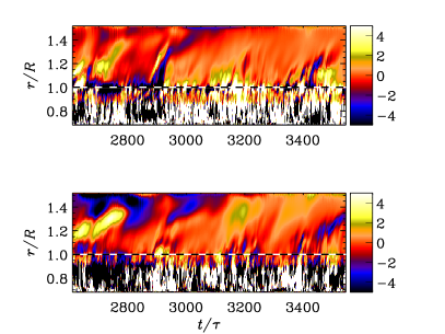
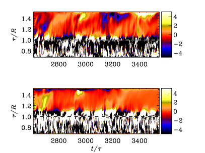
Figure 17.: Recurrence of ejections shown by plotting the dependence of the dimensionless ratio $\mu_{0}R\,\overline{\mbox{\boldmath$J$}{}\cdot\mbox{\boldmath$B$}{}}/\langle\overline{\mbox{\boldmath$B$}{}^{2}}\rangle_{t}$ on time $t/\tau$ and radius $r$ in terms of the solar radius, taken from Run A5. The top panels show a narrow band in $\theta$ in the northern hemisphere and the bottom ones in the southern hemisphere. We have also averaged in latitude from $4.1^{\circ}$ to $19.5^{\circ}$ (left panel) and $32.5^{\circ}$ to $45.5^{\circ}$ (right). Dark blue shades represent negative and light yellow positive values. The dashed horizontal lines show the location of the surface at $r=R$. Recurrence of ejections shown by plotting the dependence pjb

The ejection seen in Figures jb–eje_pt is not a single event—others follow in a recurrent fashion. However, the periodicity is not as clear as in previous work (WB,WBM). For Run A5, for example, we observe around five ejections during a time interval of about $1000$ turnover times. A clearer indication for the recurrence of the ejections can be seen in Figure pjb, where the normalized current density is averaged over two narrow latitude bands in each hemisphere. The slope of structures in the outer parts in these $rt$ diagrams gives an indication about the ejection speed $V_{\rm ej}$ which turns out to be around one solar radius in 200–250 turnover times. This translates to $V_{\rm ej}/u_{\rm rms}\approx 0.1$, which is somewhat less than the values 0.2–0.5 found for the simulations of WBM. However, the mechanism which sets the time scale of ejections is at present still unclear.

Given that gravity decreases with radius, there is in principle the possibility of a radial wind with a critical point at $r_{*}=GM/2c_{\rm s}^{2}$ (Choudhuri, 1998), which would be at $r_{*}=9.3\,R$, i.e. well outside our coronal part. Because of this and the fact that we use closed boundary conditions with no mass flux out of the domain, no such wind can occur in our simulations. Using a boundary condition that would allow a mass flux in the radial direction could change the speed and the ejection properties significantly. Including a solar-like wind in a model can have two major effects, which require a much higher amount of computational resources. The radial variation of gravity applied in these simulations implies the presence of a critical point rather close to the surface of the convection zone. Therefore, if a wind were to develop, the resulting velocity in the convection zone would be too high for a dynamo to develop; the magnetic field would be blown out too quickly. Using instead a more realistic profile for the solar wind with a position of the critical point around $r_{*}=10R$, the corresponding density stratification would be too strong to be stably resolved.

4 Conclusions

concl

In the present paper we have presented an extension of the two-layer approach of WB and WBM by including a self-consistent rotating convection zone into the model. We find a large-scale magnetic field generated by the convective turbulent motion in the convection zone. At moderate rotation rates, for a Coriolis number larger than 3, we obtain a differential rotation pattern showing super-rotation, i.e., an equator rotating faster than the poles. The dynamo solutions we find are different and some of them have a periodic oscillatory behavior, where the large-scale magnetic field does not change sign; only the strength is varying. At the maxima, the velocity is suppressed due to the backreaction via the Lorentz force. Small-scale magnetic structures seem to show an equatorward migration near the equator and a poleward one near the poles.

Using a convectively driven dynamo complicates the generation of ejections into a coronal part due to lower relative kinetic helicity. However, it was possible to produce ejections in two of the runs. The shape and the bipolar helicity structure are comparable with those of WBM. Due to the relatively high plasma $\beta$ in the outer parts of our model (compared with the solar corona), the ejections produce local minima of density which are carried along and ejected out to the top of the domain. The ejections occur recurrently, but not clearly periodically, which is similar to the Sun.

Note that our results have to be interpreted cautiously, given the use of a simplistic solar atmosphere. We neglect the effects of high temperature and low plasma $\beta$. However, we feel that the mechanism of emergence of magnetic structures driven by dynamo action from self-consistent convection may not strongly depend on these two conditions. This suggestion has to be proven in more detail in forthcoming work.

An extension of the present work would require a detailed parameter study of cause and properties of the ejections. This also includes an advanced model for the solar corona with a lower plasma $\beta$ and more efficient convection, which has a stronger stratification and is cooled by radiation. Another important aspect would be the generation of a self-consistent solar wind which supports and interacts with the ejections.

Acknowledgements

The authors thank Hardi Peter for discussion of the dynamics and rotation behavior of the solar corona. We also thank the anonymous referee for many useful suggestions. We acknowledge the allocation of computing resources provided by the Swedish National Allocations Committee at the Center for Parallel Computers at the Royal Institute of Technology in Stockholm, the National Supercomputer Centers in Linköping and the High Performance Computing Center North in Umeå. Part of the computations have been carried out in the facilities hosted by the CSC – IT Center for Science in Espoo, Finland, which are financed by the Finnish ministry of education. This work was supported in part by the European Research Council under the AstroDyn Research Project No. 227952, the Swedish Research Council Grant No. 621-2007-4064, and the Academy of Finland grants 136189, 140970 (PJK) and 218159, 141017 (MJM) as well as the HPC-Europa2 project, funded by the European Commission - DG Research in the Seventh Framework Programme under grant agreement No. 228398.

References

- Amari et al. (1999) Amari, T., Luciani, J. F., Mikic, Z., Linker, J., J. A.: 1999, Astrophys. J. 529, L49.
- Antiochos, De Vore, and Klimchuk (1999) Antiochos, S. K., De Vore, C. R., Klimchuk, J. A.: 1999, Astrophys. J. 510, 485.
- Archontis et al. (2009) Archontis, V., Hood, A. W., Savcheva, A., Golub, L., DeLuca, E.: 2009, Astrophys. J. 691, 1276.
- Badalyan (2010) Badalyan, O. G.: 2010, New Astron. 135, 143.
- Blackman and Brandenburg (2003) Blackman, E. G., Brandenburg, A.: 2003, Astrophys. J. 584, L99.
- Blackman and Field (2000a) Blackman, E. G., G. B.: 2000a, Astrophys. J. 534, 984.
- Blackman and Field (2000b) Blackman, E. G., & Field, G. B.: 2000b. Mon. Not. Roy. Astron. Soc. 318, 724.
- Brandenburg, Candelaresi, and Chatterjee (2009) Brandenburg, A., Candelaresi, S., Chatterjee, P.: 2009 Mon. Not. Roy. Astron. Soc. 398, 1414.
- Brandenburg, Moss, and Tuominen (1992) Brandenburg, A., Moss, D., Tuominen, I.: 1992, Astron. Astrophys. 265, 328.
- Brandenburg et al. (1990) Brandenburg, A., Nordlund, Å., Pulkkinen, P., Stein, R.F., Tuominen, I.: 1990, Astron. Astrophys. 232, 277.
- Brandenburg, Procaccia, and Segel (1995) Brandenburg, A., Procaccia, I., Segel, D.: 1995, Phys. Plasma 2, 1148.
- Brandenburg and Sandin (2004) Brandenburg, A., Sandin, C.: 2004, Astron. Astrophys. 427, 13.
- Brun, Browning, and Toomre (2005) Brun, A. S., Browning, M. K., Toomre, J.: 2005, Astrophys. J. 629, 461.
- Brun et al. (2004) Brun, A. S., Miesch, M. S., Toomre, J.: 2004, Astrophys. J. 614, 1073.
- Cantiello et al. (2011) Cantiello, M., Braithwaite, J., Brandenburg, A, Del Sordo, F., Käpylä, P. J., Langer, N.: 2011, IAU Symposium 272, 32.
- Choudhuri (1998) Choudhuri, A. R.: 1998, The Physics of Fluids and Plasmas, Cambridge University Press.
- Dobler, Stix, and Brandenburg (2006) Dobler, M., Stix, M., Brandenburg, A.: 2001, Astrophys. J. 638, 336.
- Elliot, Miesch, and Toomre (2000) Elliot, J. R., Miesch, M. S., Toomre, J.: 2000, Astrophys. J. 533, 546.
- Fang et al. (2010) Fang, F., Manchester, W., Abbett, W. P., van der Holst, B.: 2010, Astrophys. J. 714, 1649.
- (20) Guerrero, G., Käpylä, P. J.: 2011, Astron. Astrophys. 533, A40.
- (21) Hoeksema, J. T., Wilcox, J. M., Scherrer, P.H.: 1982, J. Geophys. Res. 87, A12.
- Hubbard and Brandenburg (2010) Hubbard, A., Brandenburg, A.: 2010, Geophys. Astrophys. Fluid Dyn. 104, 577.
- Jouve and Brun (2009) Jouve, L., Brun, A. S.: 2009, Astrophys. J. 701, 1300.
- Kaiser et al. (2008) Kaiser, M.L., Kucera, T.A., Davila, J.M., St. Cyr, O.C., Guhathakurta, M., Christian, E.: 2008, Space Sci. Rev. 136, 5.
- Käpylä, Korpi, and Brandenburg (2008) Käpylä, P. J., Korpi, M. J., Brandenburg, A.: 2008, Astron. Astrophys. 491, 353.
- Käpylä et al. (2010) Käpylä, P. J., Korpi, M. J., Brandenburg, A., Mitra, D., Tavakol, R.: 2010, Astron. Nachr. 331, 73.
- Käpylä et al. (2011) Käpylä P. J., Korpi, M. J., Guerrero, G., Brandenburg, A., Chatterjee, P.: 2011, Astron. Astrophys. 531, A162.
- Käpylä, Mantere, and Brandenburg (2011) Käpylä, P. J., Mantere, M. J., Brandenburg, A.: 2011, Astron. Nachr. 332, 883.
- Käpylä, Mantere, and Brandenburg (2012) Käpylä, P. J., Mantere, M. J., Brandenburg, A.: 2012, Astrophys. J. Lett. 755, L22.
- Kitchatinov and Rüdiger (1995) Kitchatinov, L. L., Rüdiger, G.: 1995, Astron. Astrophys. 299, 446.
- Levine, Schulz, and Frazier (1982) Levine, R. H., Schulz, M., Frazier, E. N.: 1982, Solar Phys. 77, 363.
- Li et al. (1982) Li, Y., Luhmann, J. G., Lynch, B. J., Kilpua, E. K. J.: 2011, Solar Phys. 270, 331.
- Lionello et al. (2005) Lionello, R., Riley, P., Linker, J. A., Mikić, Z.: 2005, Astrophys. J. 625, 463.
- Low (1994) Low, B. C.: 1994, Phys. Plasmas 1, 1684.
- Low (2001) Low, B. C.: 2001, J. Geophys. Res. 106, 25141.
- Low (1996) Low, B. C.: 1996, Solar Phys. 167, 217.
- Martínez-Sykora, Hansteen, and Carlsson (2008) Martínez-Sykora, J., Hansteen, V., Carlsson, M.: 2008, Astrophys. J. 679, 871.
- Miesch et al. (2000) Miesch, M. S., Elliot, J. R., Toomre, J. Clune, T. L., Glatzmaier, G. A. Gilman P. A.: 2000, Astrophys. J. 532, 59.
- Miesch, Brun, and Toomre (2006) Miesch, M. S., Brun, A. S., Toomre: 2006, Astrophys. J. 641, 618.
- Mikić, Barnes, and Schnack (1988) Mikić, Z., Barnes, D. C., & Schnack, D. D.: 1988, Astrophys. J. 328, 830.
- Mitra et al. (2009) Mitra, D., Tavakol, R., Brandenburg, A., Moss, D.: 2009, Astrophys. J. 697, 923.
- Mitra et al. (2010) Mitra, D., Candelaresi, S., Chatterjee, P., Tavakol, R., Brandenburg, A.: 2010, Astron. Nachr. 331, 130.
- Nelson et al. (2011) Nelson, N. J., Brown, B. P., Brun, A. S., Miesch, M. S., Toomre, J.: 2011, Astrophys. J. Lett. 739, L38.
- (44) Ortolani, S., Schnack, D. D.: 1993, Magnetohydrodynamics of plasma relaxation, World Scientific, Singapore.
- Ossendrijver, Stix, and Brandenburg (2001) Ossendrijver, M., Stix, M., Brandenburg, A.: 2001, Astron. Astrophys. 376, 713.
- Pesnell, Thompson, and Chamberlin (2012) Pesnell, W.D., Thompson, B.J., Chamberlin, P.C.: 2012, The Solar Dynamics Observatory (SDO).Solar Phys. 275, 3
- Pinto and Brun (2011) Pinto, R., Brun, S.: 2011, IAU Symposium 271, 393.
- Plunkett et al. (2000) Plunkett, S. P., Vourlidas, A., Šimberová, S., Karlický, M., Kotrč, P., Heinzel, P., Kupryakov, Y. A., Guo, W. P., Wu, S. T.: 2000, Solar Phys. 194, 371.
- Régnier, Amari, and Kersalé (2002) Régnier, S., Amari, T., Kersalé, E.: 2002, Astron. Astrophys. 392, 1119.
- Russev et al. (2003) Roussev, I. I., Forbes, T. G., Gombosi, T. I., Sokolov, I. V., DeZeeuw, D. L., Birn, J.: 2002, Astrophys. J. 588, L45.
- Rüdiger (1980) Rüdiger, G.: 1980, Geophys. Astrophys. Fluid Dyn. 16, 239.
- Schrijver and De Rosa (2003) Schrijver, C. J., De Rosa, M. L.: 2003, Sol. Phys. 212, 165.
- Sturrock (1980) Sturrock, P. A.: 1980, Solar Flares Colorado Associated University Press, Boulder.
- Thompson, Kliem, and Török (2011) Thompson, W. T., Kliem, B., Török, T.: 2011, Solar Phys. 276 241.
- Timothy et al. (1975) Timothy, A. F., Krieger, A. S., Vaiana, G. S.: 1975, Solar Phys. 42, 135.
- Török and Kliem (2003) Török, T., Kliem, B.: 2003, Astron. Astrophys. 406, 1043.
- Vainshtein and Cattaneo (1992) Vainshtein, S. I., Cattaneo, F.: 1992, Astrophys. J. 393, 165.
- Wang and Sheeley (1992) Wang, Y.-M., Sheeley, N. R., Jr.: 1992, Astrophys. J. 392, 310.
- Warnecke and Brandenburg (2010) Warnecke, J., Brandenburg, A.: 2010, Astron. Astrophys. 523, A19 (WB).
- Warnecke, Brandenburg, and Mitra (2011) Warnecke, J., Brandenburg, A., Mitra, D.: 2011, Astron. Astrophys. 534, A11 (WBM).
- Wiegelmann (2008) Wiegelmann, T.: 2008, J. Geophys. Res. 113, A3.
- Wöhl et al. (2010) Wöhl, H., Brajša, R., Hanslmeier, A., Gissot, S. F.: 2010, Astron. Astrophys. 520, A29.