Giant planet formation: episodic impacts vs. gradual core growth

Abstract

Context. We describe the growth of gas giant planets in the core accretion scenario.

Aims. The core growth is not modeled as a gradual accretion of planetesimals but as episodic impacts of large mass ratios, i.e. we study impacts of 0.02 - 1 $M_{\mathrm{\hbox{$\oplus$}}}$ onto cores of 1-15 $M_{\mathrm{\hbox{$\oplus$}}}$. Such impacts could deliver the majority of solid matter in the giant impact regime. We focus on the thermal response of the envelope to the energy delivery. Previous studies have shown that sudden shut off of core accretion can dramatically speed up gas accretion. We therefore expect that giant impacts followed by periods of very low core accretion will result in a net increase in gas accretion rate. This study aims at modelling such a sequence of events and to understand the reaction of the envelope to giant impacts in more detail.

Methods. To model this scenario, we spread the impact energy deposition over a time that is long compared to the sound crossing time, but very short compared to the Kelvin-Helmholtz time. The simulations are done in spherical symmetry and assume quasi-hydrostatic equilibrium.

Results. Results confirm what could be inferred from previous studies: gas can be accreted faster onto the core for the same net core growth speed while at the same time rapid gas accretion can occur for smaller cores – significantly smaller than the usual critical core mass. Furthermore our simulations show, that significant mass fractions of the envelope can be ejected by such an impact.

Conclusions. Large impacts are an efficient process to remove the accretion energy by envelope ejection. In the time between impacts, very fast gas accretion can take place. This process could significantly shorten the formation time of gas giant planets. As an important side-effect, the episodic ejection of the envelope will reset the envelope composition to nebula conditions.

1 Introduction

We study the formation of gas giant planets in the core accretion scenario (Mizuno, 1980; Pollack et al., 1996; Bodenheimer & Pollack, 1986). In this scenario, a planetary embryo grows by accreting from a swarm of planetesimals. At some point the embryo becomes massive enough to gravitationally attract a gaseous envelope. The growth process, both in terms of solid and gas accretion, is controlled by the planetesimal accretion, which is typically modeled as a gradual accretion of small planetesimals. However, in the giant collision phase under certain conditions, the accretion process could be dominated by relatively large impacts (Safronov & Zvjagina, 1969). This is confirmed by Monte-Carlo planet formation models (T. Schröter et al., in preparation) and recent results from N-body simulations (Raymond, 2005; Nimmo & Agnor, 2006). In such cases, while the collisions are less frequent, each one increases the mass of the protoplanet by a significant amount (typically of order 10%). This possibility led us to investigate the importance of the nature of the solid accretion process in the overall growth of giant planets. In particular, we want to investigate if episodic but large impacts result in changes in the mass and structure of the envelope when compared to gradual core growth?

A body of work investigates the importance of impacts and/or core luminosity on the evolution of the envelope of giant planets. One such study concerned itself with the possibility of stripping the envelope of Uranus by an impact induced shockwave (Korycansky et al., 1990). However, the authors did not follow the long-term evolution of the post impact planet and did not consider the possibility of subsequent re-accretion of gas. Ikoma et al. (2006) study the collision of two giant planets to explain the low envelope mass of HD 149026b. Another study (Anic et al., 2007) tried to assess the effect of a large impact on the long-term luminosity evolution of a giant planet with an eye on its potential detection. Other studies investigated the influence of the thermal energy content of the solid core as well as the energy provided by its contraction on the overall evolution of the luminosity (Baraffe et al., 2008). Further studies (Pečnik & Wuchterl, 2007) concern the dynamic response of proto-planetary envelopes to a perturbation within an ideal gas approach. Recently, Li et al. (2010) have studied the merger of planetary embryos focussing on the re-distribution of heavy elements following the merger.

Most closely related to the problem at hand is the sudden core luminosity shut-off scenario: the evolution of the planet when the core luminosity is suddenly shut off. This has been studied in detail by Ikoma et al. (2000) and Hubickyj et al. (2005). It is thus expected, that the periods of low core accretion in-between impacts will lead to massive gas accretion.

The effect of sporadic, relatively massive impacts during the growth phase of the core on the gas accretion has, however, not been studied in detail. Here we attempt to determine the thermal response of a gaseous envelope upon a sudden energy input delivered by a large impact to the core, and how such episodic events could modify the build-up of the envelope when compared to the nominal case of gradual accretion.

2 Material and Methods

2.1 Structure equations

In the core accretion scenario in which we place our studies, a growing giant planet is composed of a solid core surrounded by a gaseous atmosphere. To model such a structure, we solve the standard so-called equations of stellar structure. Please refer to table 6 for the explanation of all symbols. The equations are the same as in Broeg (2009), except for the envelope which is considered to be in quasi-hydrostatic equilibrium and the fact that we take into account its contraction:

$$\nabla\cdot F = \rho(\epsilon_{ac}-\dot{q}),\quad\text{or}$$

$$\frac{\partial l}{\partial r} = 4\pi r^{2}\rho(\epsilon_{ac}-\dot{q}),\quad\text{where}$$ (1)

$$\dot{q} = T\dot{s}=c_{p}\dot{T}-\frac{\delta}{\rho}\dot{P},\qquad l=4\pi r^{2}F.$$

We assume the envelope to be of solar composition and use the equation of state from Saumon et al. (1995). Following the recommended procedure for this equation of state, the effects of high-Z elements are accounted for by a somewhat enhanced He-mass fraction ($Y=0.3$).

For the opacity we use tabulated values: Pollack et al. (1985) (for $\lg T<2.3$) combined with molecular opacities from Alexander & Ferguson (1994) and high temperature opacities from Weiss et al. (1990).

2.2 Impact treatment

An impact takes place on a timescale very short compared to the evolutionary timescale of the core and envelope; compared to this timescale it is essentially instantaneous. In addition, it is not spherically symmetric – a three-dimensional analysis would be required to accurately model it and the investigation of various impact parameters would be required. Such studies, including following the evolution of the post-impact planet over several Kelvin-Helmholtz time scales are currently computationally prohibitive. We therefore opted for the study of a reduced and simplified problem: The thermal response of a spherically symmetric envelope in quasi-static equilibrium to an energy deposition onto the core corresponding to the energy delivered by the impact.

Of course, this implicitly assumes that the impactor reaches the core which is actually a good assumption for large impactors (see Li et al., 2010). The quasi-hydrostatic assumption, on the other hand, is not correct if the impact is truly instantaneous. However, provided that the envelope is not ejected by the shockwave itself, the thermal energy release of the impact energy by the core will not be instantaneous. As shown by Korycansky et al. (1990), in many cases the shockwave does not unbind a significant fraction of the atmosphere. For these situations, the major part of the impact energy is deposited directly into the core. We can very crudely estimate how fast this energy can be released by the core as follows. Assuming the projectile is spread entirely over the core, it will form a hot layer of constant thickness. For a 10 $M_{\mathrm{\hbox{$\oplus$}}}$ core and a 0.02 $M_{\mathrm{\hbox{$\oplus$}}}$ impactor and assuming a density of $5500\,\mathrm{kg/m^{3}}$ this layer will have a thickness of 10 km. A layer of depth $D$ cools over a timescale given by $\tau_{cool}=D^{2}/a$ where $a=\lambda/c_{p}\rho$ and $\lambda$ is the thermal conductivity of the material. Using typical values for the Earth mantle: $\lambda=50\,\mathrm{Wm^{-1}K^{-1}}$ (Tang & Dong, 2010), $\rho=5500\,\mathrm{kg/m^{3}}$, $c_{p}=625\,\mathrm{Jkg^{-1}K^{-1}}$ leads to a diffusion constant of $a\approx 1.5\cdot 10^{-5}\,\mathrm{m^{2}/s}$ and a corresponding cooling time of the order of $\tau_{cool}=2\cdot 10^{5}$ years.

To derive this crude estimate, we have assumed that energy was only transported by conduction and we used values for the Earth mantle. This is certainly a lower limit for the energy transport in the aftermath of the impact since other forms of energy transport are possible, especially when the core becomes partially molten and convection becomes important.

In summary we conclude that in order to simulate ’impacts’ the impact timescale must be no larger than this upper limit for the cooling time. To be on the safe side, we chose a ten times smaller value and set the impact timescale to $\tau_{imp}=10^{4}$ years.

Based on the considerations above, we simulate the energy deposition due to the impact of a large planetesimal impact by a core accretion rate $dM_{z}/dt$ modeled as a Gauss curve. We use the equivalent width $\tau_{EW}$ of the Gauss curve as the timescale of the impact. After the impact, the accretion rate is set to a low background value of $\rm 10^{-10}\,M_{\mathrm{\hbox{$\oplus$}}}/yr$. As a typical timescale we choose $10^{4}$ years. This is significantly shorter than the Kelvin-Helmholtz time scale for contraction but much larger than a dynamical timescale. Sound travel time is of the order of one year for extended protoplanets. In this way, we expect mach numbers below $1/1000$ so that a quasi-hydrostatic treatment is justified. At the same time, the impact timescale is much shorter than the Kelvin-Helmholtz time scale and the planetary envelope has to adjust its structure to the energy input much faster than it can radiate the energy away. Therefore the exact duration of the impact does not strongly affect the results. These assumptions are confirmed by the actual computations.

With the scheme described above, we can compute the thermal response of the envelope to the energy deposited into the core. Again, we do not consider the effect of the initial shock wave generate by the impact. The validity of this assumption will be further discussed in section 4.1.

2.3 Implementation

To model this scenario, we have developed a new numerical code that solves the standard equations of stellar structure (Kippenhahn & Weigert, 1990) on a self-adaptive 1-dimensional grid (Dorfi & Drury, 1987) using an implicit BDF for the time evolution. To simplify modeling mass accretion, we chose the radius $r$ as independent variable rather than mass. To handle the advection terms we use monotonized slopes after Leer (1977). The equations are discretized using a finite-volume method on a staggered mesh and the resulting non-linear equation system is solved iteratively (Henyey et al., 1964).

In the following we present the discretized equations that we use. For brevity, we omit time-centering and the advection procedure. On the staggered mesh, scalar quantities ($P,T,\rho,\Delta V$) are cell centered, and vector like quantities ($r,V,M,u,l$) grid centered. This implies different delta operators for vector and scalar quantities, see Fig. 1 for the grid layout. Averaged quantities are indicated using intermediate indices: $P_{j\pm 1/2}=\frac{1}{2}(P_{j}+P_{j\pm 1})$.

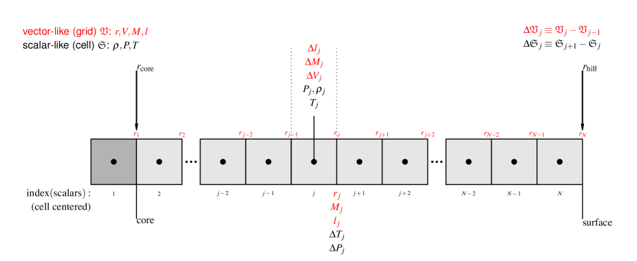
Figure 1: Layout of staggered mesh

The discretized equations are:

2.3.1 conservation of mass

$$\Delta M_{j}=\rho_{j}\Delta V_{j}$$

2.3.2 temperature gradient

$$\Delta\ln T_{j}=\nabla_{j+1/2}\Delta\ln P_{j}$$ (2)

with $\nabla$ calculated as:

$$\nabla\equiv\frac{d\ln T}{d\ln P}={\rm min}(\nabla_{\mathrm{rad}},\nabla_{\mathrm{s}}),$$ (3)

i.e. the adiabatic temperature gradient $\nabla_{\mathrm{s}}$ or the temperature gradient as caused by radiative energy transport in the diffusion approximation, $\nabla_{\mathrm{rad}}$ – whichever is smaller. This corresponds to the use of zero entropy gradient convection and the application of the Schwarzschild-criterion. $\nabla_{\mathrm{s}}$ is directly given by the equation of state, $\nabla_{\mathrm{rad}}$ is calculated as:

$$\nabla_{\mathrm{rad}}=\frac{3}{64\pi\sigma G}\,\frac{\kappa lP}{T^{4}M}$$ (4)

(see Mihalas & Weibel-Mihalas, 1999).

In detail, $\nabla_{j+1/2}$ is calculated as:

$$\nabla_{j+1/2}=\nabla(P_{j+1/2},T_{j+1/2},M_{j},l_{j})$$

$$\nabla(P,T,M,l)=\nabla\left[\nabla_{\mathrm{s}}(P,T,M,l),\nabla_{\mathrm{rad}}(P,T,M,l)\right]$$

$$\nabla(\nabla_{\mathrm{s}},\nabla_{\mathrm{rad}})=\nabla_{\mathrm{rad}}(1-\theta)+\nabla_{\mathrm{s}}\theta$$

$$\theta\equiv\frac{1}{2}\left[\tanh\left(\frac{\nabla_{\mathrm{rad}}-\nabla_{\mathrm{s}}}{\epsilon}\right)+1\right];\qquad\epsilon=10^{-4}$$

And eq (2) is discretized as:

$$[\log T_{j+1}-\log T_{j}]$$

$$- \nabla(P_{j+1/2},T_{j+1/2},M_{j},l_{j})\,[\log P_{j+1}-\log P_{j}]=0$$

2.3.3 hydrostatic equilibrium

$$4\pi r_{j}^{2}\Delta(P_{j}+P^{rad}_{j})=-G(m_{j}+M_{c})\rho_{j+1/2}\Delta V_{j+1/2}/r_{j}^{2}$$ (5)

where

$$\Delta V_{j+1/2}=\frac{4\pi}{3}(r^{3}_{j+1/2}-r^{3}_{j-1/2}),\quad\text{and}\quad P^{rad}=\frac{a}{3}T^{4}.$$

2.3.4 energy equation

In our advection scheme we make use of the connection between mass flow and relative velocity: $\widetilde{\rho}u^{rel}4\pi r^{2}=-\frac{\delta m}{\delta t}.$ The resulting equation reads:

$$\Delta\widehat{l_{j}}=-\widehat{c_{p,j}}\left\{\delta(\rho T\Delta V)_{j}/\delta t-\Delta_{j}(\widetilde{T}\frac{\delta m}{\delta t})\right\}$$

$$+\frac{\widehat{\delta_{j}}}{\widehat{\rho_{j}}}\left\{\delta(\rho P\Delta V)_{j}/\delta t-\Delta_{j}(\widetilde{P}\frac{\delta m}{\delta t})\right\}$$ (6)

where the tilde indicates quantities that are advected via van Leer monotonized slopes and the hat indicates time-centered quantities. For the results presented in this article we set the time-centering parameter $\theta=1$ (fully implicit).

2.3.5 Grid equation

The use of the radius as independent variable facilitates calculation of mass flow through the outer boundary and allows the calculation of ”detached” planets, cases for which the mass as variable becomes singular. However, within this formalism the existence of strong pressure gradients and gradients in the opacity require a self-adaptive grid which adapts to the evolving structure of the planet. We use a modified version of Dorfi & Drury (1987). The adaptive grid is defined by specifying the point concentration $n$, defined as:

$$n_{j}=\frac{\chi_{j}}{\Delta r_{j}}\quad\text{where}\quad\chi_{j}:\text{ typical scale.}$$ (7)

Setting $n_{j}$ constant implies an equidistant grid. Using a fixed scale implies an equidistant grid in linear space, using a local scale implies log-equidistant spacing. One typically takes the local average radius: $\chi_{j}=r_{j}+r_{j-1}$. The factor 0.5 is dropped because it makes no difference for the relative spacing.

More general, we want to set the local point concentration proportional to some requested resolution $\mathcal{R}$:

$$n\propto\mathcal{R}$$ (8)

One way to prescribe this proportionality in a discretized way is to set:

$$\frac{n_{j}}{\mathcal{R}_{j}}=\frac{n_{j+1}}{\mathcal{R}_{j+1}}$$ (9)

How to prescribe the resolution is a free choice. At the moment we use the length of the path in multidimensional space. Appropriate weights $g_{j}$ must be used because the different physical quantities have different physical units and can differ quite dramatically in dynamical range. We use the following required resolution:

$$\mathcal{R}_{j}^{2}=1+n_{j}^{2}\sum_{l=1}^{M}\left[g\left(\frac{\Delta f_{j}}{\overline{f_{j}}}\right)\right]_{l}$$ (10)

where the index $l$ runs over the physical quantities that should be well-resolved in path-length (i.e. mass, temperature), $(f_{j})_{l}$ represents each quantity at position $j$ on the grid, and $\bar{f}_{j}$ is the corresponding local scale (using a local average for $\overline{f_{j}}$ gives log-equidistant spacing along the path). The $g_{l}$ are the relative weights of the different physical quantities.

For the calculations presented here, we use $m,P,T$ to specify the required resolution with the weights 1.0, 0.1, and 1.0, respectively. The mean values are calculated using the harmonic mean.

While the last two equations are, in principle, sufficient to define the grid, dramatic change in resolution can occur from one grid point to the next. Since numerically this leads to significant errors, we limit limit the maximum change in spacing from one point to its direct neighbors. This is called spacial smoothing. To achieve this, we follow Dorfi and apply a diffusive process on the point density: we replace $n_{j}$ by $\hat{n}_{j}$:

$$\hat{n}_{j}=n_{j}-\alpha_{g}(\alpha_{g}+1)(n_{j-1}-2n_{j}+n_{j+1})$$ (11)

and require:

$$\frac{\hat{n}_{j}}{\mathcal{R}_{j}}=\frac{\hat{n}_{j+1}}{\mathcal{R}_{j+1}}$$ (12)

$\alpha_{g}$ gives the strength of the smoothing. To allow a maximal change of 30% from one cell to the next we set $\alpha_{g}=2$.

In addition to limiting sharp spatial change in resolution, sudden changes of the grid during time evolution need also to be avoided. For this, we use a similar procedure called temporal smoothing.

This is obtained by replacing the point density by the temporally smoothed quantity $\widetilde{n}_{j}$:

$$\widetilde{n}_{j}=\hat{n}_{j}+\frac{\tau_{grid}}{\delta t}(\hat{n}_{j}-\hat{n}_{j}^{old})$$ (13)

where $\tau_{grid}$ is the grid adaption time-scale and require instead:

$$\frac{\widetilde{n}_{j}}{\mathcal{R}_{j}}=\frac{\widetilde{n}_{j+1}}{\mathcal{R}_{j+1}}.$$ (14)

For the computations we set $\tau_{grid}=100$ years.

2.4 Boundary conditions

To specify the inner boundary condition for the core luminosity, we also integrate the gravitational potential. The equation reads:

$$r^{2}_{j+1/2}\Delta\Phi_{j}=G(m_{j+1/2}+M_{c})\Delta r_{j}.$$ (15)

In total, we have 6 non-linear equations for the unknown quantities $r,P,T,\Phi,m,l$. Due to the van Leer advection scheme, we end up with a stencil of $-3..2$, i.e. the Jacobi Matrix has a banded structure with 17 upper and 23 lower non-zero diagonals. Near the boundaries, we use donor cell advection with a stencil of $-1..1$.

For the 5 discretized differential equations we have to specify the initial values and one boundary condition per equation. For the grid equation we must specify both boundaries. In total, we need to specify 7 boundary conditions. They are:

$$r_{1} = r_{core}$$

$$m_{1} = 0$$

$$l_{1} = -\dot{M}_{z}\Phi_{1}$$

$$r_{N} = r_{hill}$$

$$P_{N} = P_{neb}$$

$$T_{N} = T_{neb}$$

$$\Phi_{N} = 0$$

where the index 1 stands for the inner boundary and $N$ for the outer. The outer radius is given by the hill radius $r_{hill}=a\sqrt[3]{{M}/({3M_{\ast}})}$; $\dot{M}_{z}$ is the accretion rate of solids. For the initial values we start with a static model at a tiny core size.

2.5 Code Verification

To verify the code we have compared the results extensively. For static models ($l=const$) we have compared to our previous, well tested, shooting method code (Broeg, 2009). The results were identical well below percent level. To test the luminosity equation, we have compared to evolutionary tracks of HD209458b of Tristan Guillot (priv. comm.) and found good agreement to 10 Gyrs. We also compared with CoRoT9b evolutionary tracks and we get a best fit for 10 Earth masses of solids in the core, again in good agreement with established calculations (Deeg et al., 2010). As a final test we have repeated the calculations of Ikoma et al. (2000) where the core accretion is stopped for a 5 $M_{\oplus}$ core, see Fig. 2.

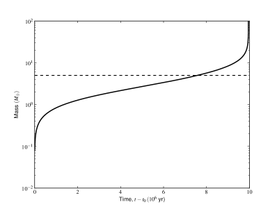
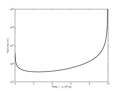
Figure 2: Time evolution of the envelope after core accretion is halted in the case of $M_{core}=5M_{\oplus}$. (a) shows the envelope mass $M_{env}$ (solid line) and the core mass $M_{core}$ (dashed line) and (b) presents the luminosity $L$. This is in good agreement with Ikoma et al. (2000), Fig. 2, even though the used opacities from Ferguson et al. (2005) (g98.7.02.tron) are not exactly equivalent.

2.6 Procedure

To study the effect of episodic impacts, we have chosen the following procedure. A planetary embryo is placed into a static minimum mass solar nebula (Hayashi, 1981) with a semi major axis of 3 AU in orbit around a sun-like star. The core grows gradually with an accretion rate of $10^{-6}\,M_{\mathrm{\hbox{$\oplus$}}}/yr$ until the impact takes place. After the impact, a period of low accretion (background rate) is assumed until a reference core undergoing gradual accretion reaches the same mass. Fig. 3 shows an example of such a time sequence.

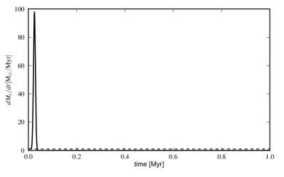
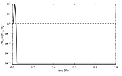
Figure 3: Simulation of one impact (here: 1 $M_{\mathrm{\hbox{$\oplus$}}}$ in $10^{4}$ yr): the core accretion rate is described by a Gaussian curve. The dashed curve shows the nominal case of constant accretion. For clarity both logarithmic and linear scale are shown.

Important parameters are the target mass, and the mass deposited by the impact. To investigate the various outcomes following changes in these parameters, we carried out a number of calculations for which we list the characteristics in Table 1. In all cases, we assumed $10^{4}$ years for the characteristic impact energy deposition timescale

Table 1: List of simulations performed with their corresponding parameters.

parameter	value
target mass	1, 2, 3, .. 15 $M_{\mathrm{\hbox{$\oplus$}}}$
impact mass	0.02, 0.1, 0.5, 1 $M_{\mathrm{\hbox{$\oplus$}}}$

except for the smallest impacts (0.01 $M_{\mathrm{\hbox{$\oplus$}}}$) for which we have used $10^{3}$ years.

We end the computations when the reference core which accretes at the nominal rate of $10^{-6}\,M_{\mathrm{\hbox{$\oplus$}}}/yr$ has reached the same mass. At this time, defined as the comparison time $t_{\mathrm{comp}}$, we compare the episodic case (EC) with the nominal case (NC). Key quantities of interest we use in this comparison are the envelope mass and the envelope accretion rate $dM_{env}/dt$.

3 Results

In this section, we present the results from our series of computations. We begin with the presentation of the data and defer the discussion to section 4. For each of the four impactor masses, we summarize the result in a table (Tables 2–5). In each table, there is one row for each target mass listing the following quantities: the NC envelope mass at $t_{\mathrm{comp}}$ ($M_{\rm env}^{0}$), the EC envelope mass compared to the NC ($M_{\rm env}/M_{\rm env}^{0}$), the NC gas accretion rate at $t_{\mathrm{comp}}$ ($dM_{\rm env}^{0}/dt$), the EC gas accretion rate ($\dot{M}_{\rm env}/\dot{M}_{\rm env}^{0}$) , the EC total luminosity compared to the NC ($L/L^{0}$), the envelope mass fraction lost ($-\Delta M_{\rm env}[\%]$), and the ratio of the impact energy to the total binding energy of the envelope ($-E_{\rm imp}/E_{b}$). The ejected envelope fraction is calculated by comparing the envelope before the impact with the smallest occurring envelope mass after the impact.

The impact energy $E_{\rm imp}$ is the gravitational energy liberated by moving the impactor from the hill sphere to the core of the target:

$$E_{\mathrm{imp}}=-\Phi(r_{c})M_{\mathrm{imp}}.$$ (16)

The total binding energy of the envelope is defined as the sum of gravitational and internal energy of the envelope:

$$E_{b}=E_{\mathrm{grav}}+E_{\mathrm{int}}\\$$ (17)

which are calculated as:

$$E_{\mathrm{grav}} = -\sum_{j=2}^{N}G\frac{M_{c}+M_{j}}{r_{j}}\rho_{j}dV_{j}$$ (18)

$$E_{\mathrm{int}} = \sum_{j=2}^{N}e(T_{j},P_{j})\,\rho_{j}dV_{j},$$ (19)

where $e$ is the internal energy as given by the equation of state. Both impact energy and binding energy are determined at the time of the impact for the yet unperturbed envelope.

Fig. 4 shows an example of the evolution of the envelope mass and gas accretion rate as a function of time for a 5 $M_{\mathrm{\hbox{$\oplus$}}}$ core having suffered an impact with a 0.1 $M_{\mathrm{\hbox{$\oplus$}}}$ impactor (solid line) and for the same core undergoing regular accretion (dashed line). At first, the impact leads to a loss of envelope mass. However, after a relatively short period in time, the accretion of gas resumes at a rate much higher than in the nominal case. By the time the nominal core reaches the same mass, the gas envelope accreted by the EC is about three times more massive. In this case the shut-off case (dotted line) accretes more gas because it reacts immediately to the shut-off of core luminosity while the gas ejection takes a certain amount of time. Afterwards, however the gas accretion rate in the EC is higher because of the slightly larger core mass.

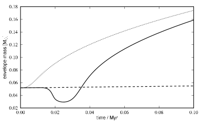
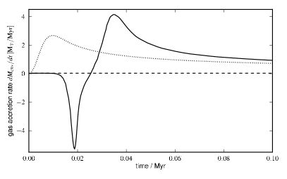
Figure 4: Accretion of 1/10 $M_{\mathrm{\hbox{$\oplus$}}}$ by a core of 5 $M_{\mathrm{\hbox{$\oplus$}}}$: envelope mass (top) and envelope accretion rate (bottom). Nominal case (constant $\dot{M}_{z}$, dashed line) vs. sudden accretion of 1/10 $M_{\mathrm{\hbox{$\oplus$}}}$ (solid line) vs. shut-off of core luminosity (dotted line). The timescale for impact and shut-off is 0.01 Myr. The offset of impact to shut-off comes from the fact that the core luminosity first rises and then decreases causing a delay. Also the mathematical prescription for core-luminosity differs slightly for shut-off and impact. In this case the shut-off case is more massive at the end. This is not so for larger impacts because the larger core mass post impact leads to larger accretion rates and eventually larger envelope mass. Note that the peak accretion rate is larger after the impact than after the shut-off.

Table 2: End-of-calculation data for impacts of 0.02 $M_{\mathrm{\hbox{$\oplus$}}}$ for different core sizes compared to nominal case (NC). The NC accretes planetesimals at a constant rate of $10^{-6}\,M_{\mathrm{\hbox{$\oplus$}}}/\rm{yr}$. Values are given at the end of computation when the core masses of nominal and science case are equal. All values are given with respect to the NC. NC values of envelope mass and envelope accretion rate are given in units of $M_{\mathrm{\hbox{$\oplus$}}}$ and $M_{\mathrm{\hbox{$\oplus$}}}/\rm{yr}$, respectively. Target mass in $M_{\mathrm{\hbox{$\oplus$}}}$. The last two columns give the ejected envelope fraction and the ratio of the impact energy to the binding energy of the envelope.

$M_{c}^{\rm target}$	$M_{\rm env}^{0}$	$M_{\rm env}/M_{\rm env}^{0}$	$dM_{\rm env}^{0}/dt$	$\dot{M}_{\rm env}/\dot{M}_{\rm env}^{0}$	$L/L^{0}$	$-\Delta M_{\rm env}[\%]$	$-E_{\rm imp}/E_{b}$
1	0.00	1.22	4.49e-09	5.7	0.0112	1.3	-272.1
2	0.01	1.58	5.73e-09	28.3	0.072	7.7	840
3	0.02	1.91	9.26e-09	52	0.182	18.9	31.3
4	0.03	1.97	1.69e-08	61.4	0.343	34.8	7.96
5	0.05	1.80	3.00e-08	63.2	0.553	50.0	2.99
6	0.09	1.54	5.05e-08	61.2	0.813	59.2	1.39
7	0.16	1.30	7.97e-08	55.6	1.11	45.2	0.74
8	0.26	1.12	1.24e-07	48.4	1.4	26.5	0.433
9	0.41	1.01	1.81e-07	39	1.58	15.6	0.272
10	0.63	0.97	2.64e-07	23.7	1.55	9.1	0.179
11	0.96	0.96	3.76e-07	12.5	1.4	5.3	0.122
12	1.43	0.97	5.60e-07	5.79	1.24	2.9	0.0853
13	2.16	0.98	8.92e-07	2.41	1.13	1.3	0.0602
14	3.39	0.98	1.65e-06	1	1.06	0.3	0.0421
15	6.49	0.97	5.96e-06	0.866	0.999	0.0	0.0266

Table 3: End-of-calculation data for impacts of 0.1 $M_{\mathrm{\hbox{$\oplus$}}}$. Same conventions as Table 2.

$M_{c}^{\rm target}$	$M_{\rm env}^{0}$	$M_{\rm env}/M_{\rm env}^{0}$	$dM_{\rm env}^{0}/dt$	$\dot{M}_{\rm env}/\dot{M}_{\rm env}^{0}$	$L/L^{0}$	$-\Delta M_{\rm env}[\%]$	$-E_{\rm imp}/E_{b}$
1	0.00	1.42	4.54e-09	3.25	0.00674	0.0	-1.36e+03
2	0.01	2.16	5.92e-09	14.8	0.0378	4.9	4.2e+03
3	0.02	2.83	9.62e-09	26	0.0918	15.3	157
4	0.03	3.07	1.75e-08	30.1	0.169	29.6	39.8
5	0.05	2.90	3.17e-08	29.4	0.271	43.3	15
6	0.10	2.55	5.29e-08	28.6	0.398	53.7	6.95
7	0.17	2.19	8.45e-08	26.2	0.549	60.8	3.7
8	0.27	1.86	1.28e-07	24.8	0.727	64.6	2.17
9	0.43	1.59	1.89e-07	23.2	0.929	61.8	1.36
10	0.66	1.37	2.68e-07	21.8	1.15	50.6	0.893
11	0.99	1.20	3.88e-07	19.2	1.36	36.1	0.61
12	1.48	1.08	5.77e-07	16.2	1.55	24.1	0.426
13	2.23	0.99	9.23e-07	11.7	1.66	15.1	0.301
14	3.53	0.94	1.75e-06	5.79	1.55	8.1	0.21
15	7.06	0.91	7.39e-06	1.23	1.13	0.0	0.133

Table 4: End-of-calculation data for impacts of 0.5 $M_{\mathrm{\hbox{$\oplus$}}}$. Same conventions as Table 2. An asterisk indicates premature end of calculation due to rapid gas accretion.

$M_{c}^{\rm target}$	$M_{\rm env}^{0}$	$M_{\rm env}/M_{\rm env}^{0}$	$dM_{\rm env}^{0}/dt$	$\dot{M}_{\rm env}/\dot{M}_{\rm env}^{0}$	$L/L^{0}$	$-\Delta M_{\rm env}[\%]$	$-E_{\rm imp}/E_{b}$
1	0.01	2.73	4.91e-09	2.33	0.00537	0.1	-6.79e+03
2	0.01	4.71	7.02e-09	6.7	0.0186	6.0	2.1e+04
3	0.02	6.16	1.23e-08	9.38	0.0404	17.6	783
4	0.04	6.56	2.24e-08	10.4	0.072	34.0	199
5	0.07	6.20	3.93e-08	10.7	0.115	50.2	74.8
6	0.12	5.57	6.33e-08	10.8	0.172	62.8	34.8
7	0.20	4.93	9.99e-08	10.8	0.247	71.5	18.5
8	0.33	4.37	1.48e-07	11.4	0.346	77.4	10.8
9	0.51	3.92	2.20e-07	11.7	0.479	81.4	6.79
10	0.77	3.55	3.13e-07	12.7	0.664	84.4	4.46
11	1.16	3.27	4.54e-07	14	0.948	86.7	3.05
12	1.74	3.07	6.94e-07	16.5	1.46	88.5	2.13
13	2.65	3.01	1.16e-06	21.3	2.87	89.0	1.51
14	4.40	5.03	2.56e-06	152	32.8	80.8	1.05
15	*12.28	*11.79	*4.64e-05	*3.41e+06	* 104	* 52.6	* 0.7

Table 5: End-of-calculation data for impacts of 1 $M_{\mathrm{\hbox{$\oplus$}}}$. Same conventions as Table 2. An asterisk indicates premature end of calculation due to rapid gas accretion.

$M_{c}^{\rm target}$	$M_{\rm env}^{0}$	$M_{\rm env}/M_{\rm env}^{0}$	$dM_{\rm env}^{0}/dt$	$\dot{M}_{\rm env}/\dot{M}_{\rm env}^{0}$	$L/L^{0}$	$-\Delta M_{\rm env}[\%]$	$-E_{\rm imp}/E_{b}$
1	*0.01	*4.84	*5.71e-09	*2.97	*0.00729	* 0.0	* -13602.5
2	0.02	7.41	9.11e-09	5.57	0.0188	6.1	4.2e+04
3	0.03	8.82	1.68e-08	6.81	0.0371	17.8	1.57e+03
4	0.05	8.92	2.99e-08	7.4	0.0638	34.3	398
5	0.09	8.34	5.03e-08	7.92	0.102	50.8	150
6	0.16	7.62	7.95e-08	8.57	0.156	63.6	69.5
7	0.26	6.99	1.22e-07	9.37	0.236	72.6	37
8	0.41	6.56	1.79e-07	11.1	0.365	78.6	21.7
9	0.63	6.46	2.62e-07	14.8	0.601	82.9	13.6
10	0.95	6.81	3.74e-07	25.1	1.33	85.9	8.93
11	1.42	11.06	5.57e-07	153	10.5	88.3	6.1
12	*1.95	*76.20	*7.90e-07	*2.01e+08	* 790	* 90.2	* 4.3
13	*2.77	*53.12	*1.22e-06	*1.3e+08	* 617	* 91.9	* 3.0
14	*4.30	*33.88	*2.44e-06	*6.49e+07	* 482	* 93.4	* 2.1
15	*11.21	*12.84	*3.27e-05	*4.52e+06	*2.48e+03	* 93.1	* 1.3

For the most energetic impacts, Fig. 5 shows the envelope mass and its accretion rate using different colors for all different targets. For comparison, the NC is displayed as a dashed line. The envelope mass as a function of core mass is represented in the upper panel. We note that in all cases, the final envelope mass is significantly larger than in the NC. The lower panels show the gas accretion rate. Obviously, this assumed nominal rate has no relation with physical reality, it only serves the purpose to compare cores after they have accreted the same amount of mass. In this figure one can see that, after an initial phase of mass loss, the gas accretion rates stay always larger than the NC values in all cases. For core masses between 12 to 15 $M_{\mathrm{\hbox{$\oplus$}}}$, the impacts can even trigger rapid gas accretion while the corresponding NC core has not yet reached its critical mass.

In the introduction we have said that rapid gas accretion after the impact can be expected by analogy of the well studied shut-off scenario. Our calculations confirm this. The clearly new and unexpeced result of this study is the almost complete ejection of envelope and the very fast reaccretion thereof after the impact. This has strong implications for the composition of the envelope.

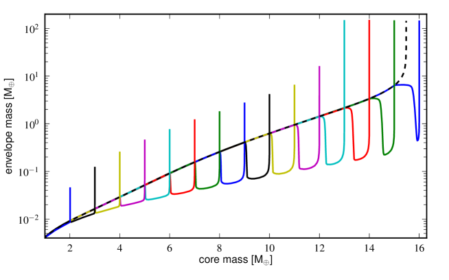
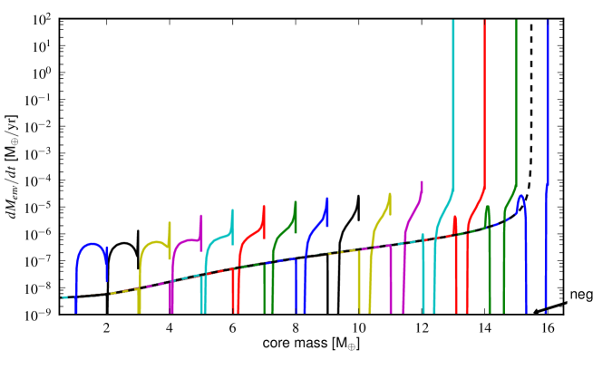
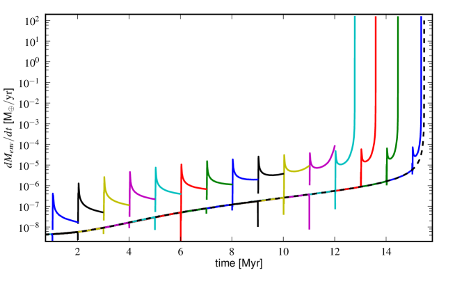
Figure 5: Envelope mass and gas accretion rate following impacts of 1 $M_{\mathrm{\hbox{$\oplus$}}}$. The calculations with core masses 12-15 end prematurely because gas accretion becomes supersonic. The dashed line represents the NC in all panels. The lower panels show the gas accretion rate in log-scale. Note that all values below $10^{-9}$ actually become negative. The lowest panel shows the envelope accretion rate as a function of time – the constant core accretion rate was used to convert the core mass to a proxy time. Each color represents a different planet having an impact that has evolved to this point by constant core growth.The very high accretion rate directly after the impact is similar to the shut-off case. In case of shut-off the accretion rate rises immediately but in the impact case, the impact and ejection causes a delay (not visible on this scale). Afterwards the evolution is practically identical. For large impacts, the henceforth larger core mass leads to a significantly higher accretion rate when compared to the shut-off case.

4 Discussion

We present a series of computations that aim at exploring the case in which episodic large bodies rather than a steady state of small ones provide the bulk of the core mass accretion. The resulting envelope structure, in particular the mass of the envelope, is compared between the two cases at a time when both cores have acrreted the same mass. We find that the large impacts or sudden energy input, while briefly reducing the envelope mass, allow for a larger gas accretion rate leading for all sizable impactors to a significantly more massive envelope. The resulting mass of the envelope normalized by the one obtained in the NC is listed in column 3 of Tables 2-5. Furthermore, the envelope is not only more massive but the gas accretion rate is also larger (column 5 of the tables) indicating that the difference will keep growing. The exceptions are very small impacts on relatively large cores (0.1 $M_{\mathrm{\hbox{$\oplus$}}}$ on 13-15 $M_{\mathrm{\hbox{$\oplus$}}}$ cores and 0.02 $M_{\mathrm{\hbox{$\oplus$}}}$ onto 10-15 $M_{\mathrm{\hbox{$\oplus$}}}$ cores). In these cases, the impacts have little to no effect.

To understand the reason for this, we focus on the most dramatic 1 $M_{\mathrm{\hbox{$\oplus$}}}$ impact case. Figure 6 shows the envelope mass for all different targets over 6 impact timescales. But now, time is plotted on the abscissa and we restrict the plot to 6 times the impact timescale. Each solid line stands for one target, the lines are labelled with the core masses. The dashed line shows the core luminosity in arbitrary units, to show the duration of the impact effects.

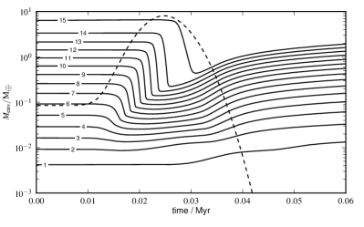
Figure 6: Envelope mass around the time of the impact for a 1 $M_{\mathrm{\hbox{$\oplus$}}}$ impact. The numbers give the target core mass in $M_{\mathrm{\hbox{$\oplus$}}}$ and the dashed line shows the core luminosity in arbitray units ($10^{21}$ W) to show when the ”impact” takes place.

For small envelopes very little happens. Only after the impact, when the core luminosity becomes tiny, does the envelope mass increase slightly. In this case the envelope is so thin that the energy deposited can be transported very efficiently, therefore having no effect on the structure. As the envelope becomes more massive, the energy input starts to eject part of the envelope – a significant fraction for envelopes larger than $3\cdot 10^{-3}\,$$M_{\mathrm{\hbox{$\oplus$}}}$ or cores larger than 3-4 $M_{\mathrm{\hbox{$\oplus$}}}$. This effect becomes stronger as the envelope considered is more massive. One can also see, that a more massive envelope is ejected later in time. The reason for this is that it takes more time to inject enough energy to remove the envelope. In this case, the impact energy is always larger than the binding energy of the envelope. Therefore we eject a larger envelope fraction for larger envelopes because the energy transport becomes less efficient – the energy is trapped in the envelope and can be used to remove it.

This is not always the case for smaller impacts, however. Consider the 0.1 $M_{\mathrm{\hbox{$\oplus$}}}$ impact case, Fig. 7.

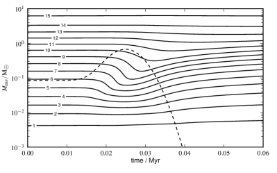
Figure 7: Same as Fig. 6 but for ten times smaller impacts (0.1 $M_{\mathrm{\hbox{$\oplus$}}}$)

Starting with small envelopes, the behavior is similar. Only when the envelope reaches a certain size, the envelope is partially ejected. More so for more massive envelopes. Nevertheless, the behaviour changes for very massive envelopes: less envelope is ejected and eventually the impact has little effect. The reason is simple: starting at cores of 10 $M_{\mathrm{\hbox{$\oplus$}}}$ and larger, the impact energy is smaller than the total binding energy of the envelope (see Table 3). Therefore, while the process is efficient in terms of using the available energy, there is not enough energy available and only a fraction of the envelope can be removed from the gravitational potential of the core and envelope. The amount of available energy for all calculations is shown in Fig. 8.

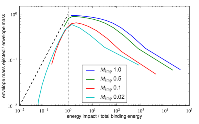
Figure 8: Fraction of envelope mass ejeced by the impact as a function of available energy. The abscissa shows the ratio of impact energy to total binding energy of the envelope. Left of the vertical dashed line the impact energy is insufficient to remove the entire envelope. The other dashed line shows the ejected mass ratio for 100% efficient processes. Note that large target cores are to the left, small targets to the right.

The largest impactor provides enough energy for all target configurations, whereas the smaller impactors have insufficient energy to eject the most massive envelopes completely. The dashed line shows the enjected mass ratio for 100% efficient processes. If the energy of the impact is orders of magnitude larger than the binding energy, this implies small targets with tiny envelopes. The impact energy can be transported effecively and the envelope ejection becomes small. That is why the curves go down again. In this regime the impact shockwave might be efficient in removing the entire envelope and a hydrodynamic treatment might be necessary (see section 4.1). For giant planet formation, this is not a very interesting regime, however.

We have already said that the final envelope mass at $t_{\mathrm{comp}}$ is larger in the EC. To study this in more detail, we consider Fig. 9. It shows the ratio of the envelope mass in the EC to the NC (ratio $M_{env}$). The comparison time is chosen so that EC and NC have equal core mass.

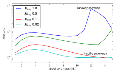
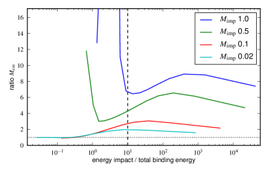
Figure 9: Ratio of post-impact envelope mass to the NC envelope mass after the impact at $t_{\mathrm{comp}}$ (same core mass). All computed impactors and target sizes are shown. top: abscissa shows the target core mass. Both large impactors provide sufficient energy to overcome the envelope binding energy for all targets. For the larger cores, runaway gas accretion is triggered. The smaller impacts do not have enough energy to significantly affect the large targets. bottom: abscissa shows impact energy as fraction of the total binding energy. Left of the vertical dashed line, the impact shockwave is not capable of ejecting the envelope directly (assuming that 10% of the impact energy directly heats the envelope).

The top panel shows the envelope ratio vs. target core mass. For small cores, this ratio rises with increasing core mass. For large cores, runaway gas accretion can be triggerd if enough energy is available to remove a large envelope fraction. If the energy is insufficient, the envelope ratio decreases again. But only in the case of the smallest impactor does it go below 1.

After discussing the energetics of the envelope removal, we consider the acceleration of gas accretion. Only if the time for re-accretion of the ejected gas is small compared to the periods in-between impacts (the shut-off-like phase) we have a resulting net speed-up. Why is the ejected gas replaced so fast? It turns out that the initial envelope loss is a key factor. The gas accretion is governed by the rate by which the energy can be radiated away. For sub-critical cores, the luminosity or planetesimal accretion rate sets the internal structure of the envelope and in the static limit directly the total envelope mass. When an impact occurs, the energy is used to eject a large fraction of the envelope and the remaining energy is radiated away very fast due to the high luminosity. The high luminosity is possible because of the tiny envelope. Afterwards, the core luminosity is low and gas accretion can be very fast. All the accretion energy that is evenly spread out in the NC has been radiated away or used to eject the envelope. Figure 10 shows the time evolution of the

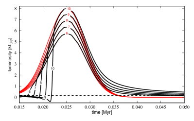
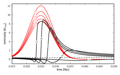
Figure 10: Luminosity during impacts of 1 $M_{\mathrm{\hbox{$\oplus$}}}$ for target core sizes from 6-10 $M_{\mathrm{\hbox{$\oplus$}}}$ (top) and 11-15 $M_{\mathrm{\hbox{$\oplus$}}}$ (bottom). The thick black line shows the total luminosity and the thin red lines show the core luminosities. Small labels indicate the target core mass in $M_{\mathrm{\hbox{$\oplus$}}}$. For reference, the dashed line shows the nominal case of gradual core growth for the most massive target.

luminosity for 0.5 $M_{\mathrm{\hbox{$\oplus$}}}$ impacts onto intermediate cores. It shows both the initial decrease in total luminosity $L$, and the very large value of $L$ shortly afterwards. After the envelope has expanded, and after the impact energy has been transported to the surface, the luminosity is mainly produced by contraction of the envelope. Therefore the luminosity quickly shrinks to and below the nominal value representing constant core accretion. This is not visible in Fig. 10 because the figure only shows the first 0.1 Ma after the impact to resolve the luminosity curve. Afterwards, there is still a long time (in this case 0.5 Myr) to accrete envelope gas with a very small core luminosity.

For more extended envelopes, another effect comes into play: the binding energy of the envelope. When the mass of the envelope becomes important, injecting energy at the center of the planet will not lead to an increase of temperature. On the contrary, it will actually reduce the temperature after a very brief temperature increase. This is caused by the negative gravothermal specific heat which is well-known for stars where is is responsible for stable hydrogen burning. When nuclear energy production suddenly increases, the temperature will decrease and reduce the nuclear energy production. Following Kippenhahn & Weigert (1990) (section 25.3.4) we define the gravothermal specific heat as:

$$c^{*}=c_{P}\left(1-\nabla_{s}\frac{4\delta}{4\alpha-3}\right)$$

where $c_{P}$ is the specific heat at constant pressure and $\alpha$ and $\delta$ are the generally used logarithmic derivatives in the equation of state of density vs. pressure or temperature, respectively. If $c^{*}$ is negative, adding energy $dq$ to the gas will reduce its temperature: more energy is needed for the expansion of the envelope than what is originally the cause for the expansion. Applying this definition to our envelope structures prior to impact shows that $c^{*}$ is indeed negative for the central part of the envelopes. The effect is even stronger for gas giant planets than for stars (of comparable size), because the gravitational field of the core enhances the effect that is only caused by the self-gravity of the gas for stars. In our calculations, this effect can be seen by the decrease in luminosity in the initial impact phases. For massive envelopes, this effect is so strong that a temperature inversion happens in the outer envelope and the total luminosity becomes negative for a short time. During this phase, the planet cannot radiate its internal energy away. But this phase lasts only a very short time (e.g., 1200 yr in the $M_{c}=8$ $M_{\mathrm{\hbox{$\oplus$}}}$, 1 $M_{\mathrm{\hbox{$\oplus$}}}$ impact case). After this phase, the planet is relatively cold and can accrete gas faster than before the impact.

This is the reason why the lost envelope mass can be replaced with new gas so fast that the envelope ejection has no important consequences for the evolution of the planet, see section 4.2.

4.1 Consequences of the impact shock

A realistic impact for relatively small envelopes that we are considering can be divided in the following stages: 1) the impactor traverses the envelope and deposits some energy directly in all layers. 2) The impactor hits the core and deposits a fraction of its energy directly in the lower layers of the envelope. This causes a blast wave to travel through the envelope. 3) The energy deposited in or around the core is transported to the envelope and the envelope reacts to this. 4) After the impact energy has been processed, the envelope reacts to the decreased energy flux and typically contracts.

In our computation, we neglect stage 1. Stages 2 and 3 are modelled together in a simplified fashion by assuming that the energy is released on a certain timescale. Test calculations show that the the reaction of the envelope does not depend strongly on the exact value of this timescale as long as two things are true: it is much longer than a dynamic timescale so that the envelope has enough time to stay in hydrostatic equilibrium. Secondly, the timescale must be much shorter than the cooling timescale. This means that there is no time for the envelope to radiate the energy during the ”impact”. Stage 4, the gas accretion after the ”impact” is modelled consistently.

This treatment neglects the fact that, for large impacts, stage 2 can dynamically strip the envelope. This has been shown by Korycansky et al. (1990, h.f. KOR90). We have also begun to simulate this impact with 3-dimensional SPH simulations using dunite for the core and ideal gas for the envelope. We were using a SPH formulation suitable for handling high density contrasts. Our calculations show a gradual change from no ejection to full ejection of envelope and a strong dependence on impact paramenter: Large impact angles are more likely and tend to eject less envelope. We will study this in detail in a forthcoming article (A. Reufer et al., in prep.). Nevertheless, it appears clear that for giant impacts significant fractions of the envelope can be ejected, especially on smaller targets. However, in such a case, impact energies are large and subsequently stage 3 will continue to eject the (remaining) envelope and prevent envelope accretion due to huge luminosity until stage 3 has ended and core luminosity drops back to ’normal’ levels. Afterwards the behaviour will be similar independent of the amount of gas ejected already during stage 2. Therefore we argue that the mid- and long-term outcome will be independent of the exact nature of envelope ejection. Note that during stage 3, near the peak core luminosity, the envelope is again in a static state with $l=const$ throughout the envelope in most cases (see Fig. 10). This means that it has ’forgotten’ its history and previous envelope ejection – by blast wave or otherwise – is irrelevant.

4.2 Comparison with a stop of core accretion

Ikoma et al. (2000) and Hubickyj et al. (2005) have already studied the effect of shutting off core accretion on the gas accretion rate. Here we compare the impact to core luminosity shut-off. Figure 11

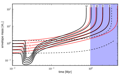
Figure 11: Gas accretion compared to shutdown scenario. Black lines show the envelope mass after 1 $M_{\mathrm{\hbox{$\oplus$}}}$ impacts on cores of 8 - 12 $M_{\mathrm{\hbox{$\oplus$}}}$. Red lines show the evolution when the core accretion rate is simply shut off with the same timescale and to the same background rate instead of impacting 1 $M_{\mathrm{\hbox{$\oplus$}}}$. Dashed lines show the envelope mass of the NC for the largest and smallest target. At 1 Myr the NC and the impact case have the same core size. Cases 8-11 have been extended beyond the 1 Myr $t_{\mathrm{comp}}$ that was usually adopted to compare to the NC.

shows core masses in the range from 8 to 12 $M_{\mathrm{\hbox{$\oplus$}}}$ and the evolution of the envelope mass in 1) the impact case and 2) when turning off core accretion. We use the same timescale of $10^{4}$ years to reduce the core accretion rate to the background level. To allow a direct comparison, we have extended the old calculations to later times to see when the planets start rapid gas accretion. The solid lines show the impact scenario, while the red lines represent shutdown of core accretion.

It is evident, that the shutdown leads to a quicker envelope build-up initially. The impact cases first expand and loose a significant mass fraction. After the envelope loss, however, the impact cases quickly gain envelope mass, much faster than the shutdown case. At all times after the initial ejection, the envelope accretion rate stays larger for the impact case. For the comparison it is important to note that the impact case has a heavier core by 1 $M_{\mathrm{\hbox{$\oplus$}}}$ compared to the shutdown case. When comparing with shutdown cases 1 Myr later (having the same core size), the envelope accretion rates become similar only after the planet has ”forgotten” the impact. This occurs after a few Kelvin-Helmholtz timescales. In the end the planets reach an envelope mass of the same size as the respective larger core in the shutdown case.

In other words, the impact scenario allows gas accretion at a slightly enhanced rate compared to the shutdown case while concurrently growing the core. When comparing cores of equal size, the impact case is almost as fast as the shutdown case. Only for very large cores, when the time-to-runaway in the shutdown case is of the order of 1 Myr or less (i.e. the time it takes to gradually increase the core by the size of the impactor is longer than the time to reach rapid gas accretion), is the impact case slower than the shutdown case. For long stretches between impacts, the absence of core accretion is the important effect but the reconfiguration of the envelope during the impact plays an important role shortly after the impact. Hence, when the times between impacts are relatively short, the impact case is still faster than the shutdown case (for equal initial core mass). This is only changed when the time between impacts becomes so short, that the initial mass loss cannot be compensated anymore.

5 Conclusion

We have analyzed the effect of relatively massive impacts onto the cores of giant planets in the growth phase. Previous studies (Ikoma et al., 2000; Hubickyj et al., 2005) have shown how the envelope reacts to a shut-off of core luminosity with rapid envelope accretion. Therefore, intermittent giant impacts with long periods of very low core accretion in-between are expected speed up gas accretion. The aim of this study was to study the reaction of the envelope to the giant impact and the subsequent period of low core luminosity in detail. Wether or not a net acceleration of gas accretion takes place and how strong this effect is, depends on the timescale of the reaction to the impact in relation to the time in-between impacts.

There are two major effects: 1) Due to a very large core luminosity after the impact, a large fraction of the envelope is ejected. The remaining tiny envelope allows a very fast energy transport and in consequence the huge impact energy is used up or radiated away very fast. The huge luminosity in combination with a small envelope leads to a small Kelvin-Helmholtz time. Therefore the envelope ’forgets’ that the impact has taken place in very short time. Afterwards, very little solid accretion is necessary for a given net core growth speed and the subsequent evolution up to the next impact can be understood by the well-studied sudden shut-off of core luminosity. However, due to the episodic impacts, further core growth is still possible. 2) This effect is enhanced by a second: The very large luminosity during the impact reconfigures the envelope structure so that it is in hydrostatic equilibrium for very high energy fluxes. Shutting off core accretion after this reconfiguration triggers higher gas accretion rates than the shut-off without prior impact. This can also be understood in terms of the negative gravothermal specific heat of self-gravitating non-degenerate gases. In this state the impacts actually lower the central temperature which explains why subsequent gas accretion can be faster after the impact. This second effect helps reduce the time it takes to accrete once more the envelope gas that has been ejected by the impact. Once the planet has again the same envelope mass as before the impact but a much lower core luminosity, the evolution follows the shutdown scenario.

Together, the alternation between very high and low energy input allows more gas to be accreted even though the impact initially ejects some (or all) of the envelope gas. The subsequent high gas accretion rate quickly reforms the original envelope and continues to accrete faster than the gradually growing case. In this way, even a rapid succession of impacts can lead to a faster envelope growth.

A further interesting consequence of the envelope loss caused by the impact relates to the dust opacity: every time the envelope is ejected, new fresh gas is accreted from the nebula, therefore resetting any former modifications to the opacity caused by e.g. dust growth and settling.

In summary, we find that episodic large impacts significantly speed up gas accretion as was expected from shut-off calculations. The new result of this study is the fact that 1) almost the entire envelope of the planet is ejected as a consequence of the impact energy and 2) it takes only a very short time to accrete the lost gas after the ejection. In fact, this is so fast that the ejection has practically no effect on the long-term evolution - envelope masses are equivalent with the shutdown-case using the increased post-impact core mass.

We can therefore conclude the following for the formation of giant planets: If planetesimals are accreted in a regime where mass ratios are large, i.e. most mass is delivered by massive impacts, this will accelerate envelope build-up. Furthermore, the ratio of envelope to core mass will be significantly enhanced and smaller cores can begin rapid gas accretion while the core is growing by large impacts. The speedup with consecutive impacts, can be understood in principle from these calculations. We will study a full evolution calculation based on episodic core growth in a future publication.

Appendix A List of symbols

Table 6: List of symbols

name	unit	description
$\lx@intercol a\hfil$	m	semi major axis
$\lx@intercol a\hfil$	$\rm J\,m^{-3}\,K^{-4}$	radiation constant
$\lx@intercol c_{P}\hfil$	$\rm J\,kg^{-1}\,K^{-1}$	specific heat at constant pressure
$\lx@intercol\epsilon_{ac}\hfil$	$\rm J\,kg^{-1}\,s^{-1}$	energy in-flux from planetesimal accretion per unit mass
$\lx@intercol F\hfil$	$\rm W\,m^{-2}$	energy flux
$\lx@intercol\Phi\hfil$	$\rm J\,kg^{-1}$	gravitational potential
$\lx@intercol\delta\hfil$	1	equation of state: $\delta\equiv-\partial\ln\rho/\partial\ln T|_{P}$
$\lx@intercol G\hfil$	$\rm N\,m^{2}\,kg^{-2}$	gravitational constant
$\lx@intercol\kappa\hfil$	$\rm m\,kg^{-1}$	Rosseland-mean opacity
$\lx@intercol l\hfil$	$\rm W\,m^{-2}$	luminosity
$\lx@intercol m\hfil$	kg	envelope mass
$\lx@intercol M_{c}\hfil$	kg	core mass
$\lx@intercol M_{\ast}\hfil$	kg	host star mass
$\lx@intercol n\hfil$	1	point concentration
$\lx@intercol\nabla\hfil$	1	log. temperature gradient $d\ln T/d\ln P$
$\lx@intercol\nabla_{s}\hfil$	1	isentropic temperature gradient $d\ln T/d\ln P|_{s}$
$\lx@intercol P\hfil$	Pa	pressure
$\lx@intercol q\hfil$	$\rm J\,kg^{-1}$	heat per unit mass
$\lx@intercol T\hfil$	K	temperature
$\lx@intercol r\hfil$	m	radius
$\lx@intercol\rho\hfil$	$\rm kg\,m^{-3}$	density
$\lx@intercol\sigma\hfil$	$\rm W\,m^{2}\,K^{-4}$	Stefan-Boltzmann constant
$\lx@intercol t\hfil$	s	time
$\lx@intercol\tau_{EW}\hfil$	s	impact timescale (equivalent width of Gaussian)
$\lx@intercol\theta\hfil$	1	time centering parameter 0..1
$\lx@intercol u_{rel}\hfil$	$\rm m/s$	relative velocity of matter with respect to grid: $u_{rel}+u_{grid}=u$
$\lx@intercol V\hfil$	$\rm m^{3}$	volume
$\lx@intercol e\hfil$	$\rm J\,kg^{-1}$	specific internal energy per unit mass

Table 7: Operators

operator	description	definition
$\delta$	temporal delta	$\delta x=x^{new}-x^{old}$
$\Delta$	spacial delta on scalar	$\Delta S_{j}=S_{j+1}-S_{j}$
	spacial delta on vector	$\Delta v_{j}=v_{j}-v_{j-1}$
$\widehat{\hskip 4.30554pt}$	time-centering	$\widehat{x}=\theta x^{new}+(1-\theta)x^{old}$
$\widetilde{\hskip 4.30554pt}$	advection	donor cell: take upstream value

Table 8: List of non SI units with adopted values

unit	description	value
$M_{\mathrm{\hbox{$\oplus$}}}$	mass of Earth	5.9742e24 kg
$L_{\mathrm{jup}}$	Jupiter internal luminosity	3.35e17 W
yr	julian year	31557600 s

References

- Alexander & Ferguson (1994) Alexander, D. R. & Ferguson, J. W. 1994, ApJ, 437, 879
- Anic et al. (2007) Anic, A., Alibert, Y., & Benz, W. 2007, A&A, 466, 717
- Baraffe et al. (2008) Baraffe, I., Chabrier, G., & Barman, T. 2008, A&A, 482, 315
- Bodenheimer & Pollack (1986) Bodenheimer, P. & Pollack, J. B. 1986, Icarus, 67, 391
- Broeg (2009) Broeg, C. H. 2009, Icarus, 204, 15
- Deeg et al. (2010) Deeg, H. J., Moutou, C., Erikson, A., et al. 2010, Nature, 464, 384
- Dorfi & Drury (1987) Dorfi, E. A. & Drury, L. O. 1987, J. Comput. Phys., 69, 175
- Ferguson et al. (2005) Ferguson, J. W., Alexander, D. R., Allard, F., et al. 2005, ApJ, 623, 585
- Hayashi (1981) Hayashi, C. 1981, Progress of Theoretical Physics Supplement, 70, 35
- Henyey et al. (1964) Henyey, L. G., Forbes, J. E., & Gould, N. L. 1964, ApJ, 139, 306
- Hubickyj et al. (2005) Hubickyj, O., Bodenheimer, P., & Lissauer, J. J. 2005, Icarus, 179, 415
- Ikoma et al. (2006) Ikoma, M., Guillot, T., Genda, H., Tanigawa, T., & Ida, S. 2006, ApJ, 650, 1150
- Ikoma et al. (2000) Ikoma, M., Nakazawa, K., & Emori, H. 2000, ApJ, 537, 1013
- Kippenhahn & Weigert (1990) Kippenhahn, R. & Weigert, A. 1990, Stellar Structure and Evolution, ed. M. Harwit, R. Kippenhahn, V. Trimble, & J.-P. Zahn, Astronomy and Astrophysics Library (Berlin, Heidelberg: Springer-Verlag)
- Korycansky et al. (1990) Korycansky, D. G., Bodenheimer, P., Cassen, P., & Pollack, J. B. 1990, Icarus, 84, 528
- Leer (1977) Leer, B. V. 1977, Journal of Computational Physics, 23, 276
- Li et al. (2010) Li, S. L., Agnor, C. B., & Lin, D. N. C. 2010, ApJ, 720, 1161
- Mihalas & Weibel-Mihalas (1999) Mihalas, D. & Weibel-Mihalas, B. 1999, Foundation of Radiation Hydrodynamics (Dover Books)
- Mizuno (1980) Mizuno, H. 1980, Progress of Theoretical Physics, 64, 544
- Nimmo & Agnor (2006) Nimmo, F. & Agnor, C. B. 2006, EPSL, 243, 26
- Pečnik & Wuchterl (2007) Pečnik, B. & Wuchterl, G. 2007, MNRAS, 381, 640
- Pollack et al. (1996) Pollack, J. B., Hubickyj, O., Bodenheimer, P., et al. 1996, Icarus, 124, 62
- Pollack et al. (1985) Pollack, J. B., McKay, C. P., & Christofferson, B. M. 1985, Icarus, 64, 471
- Raymond (2005) Raymond, S. N. 2005, PhD thesis, University of Washington
- Safronov & Zvjagina (1969) Safronov, V. S. & Zvjagina, E. V. 1969, Icarus, 10, 109
- Saumon et al. (1995) Saumon, D., Chabrier, G., & van Horn, H. M. 1995, ApJS, 99, 713
- Tang & Dong (2010) Tang, X. & Dong, J. 2010, Proceedings of the National Academy of Sciences, 107, 4539
- Weiss et al. (1990) Weiss, A., Keady, J. J., & Magee, N. H. 1990, Atomic Data and Nuclear Data Tables, 45, 209