Effects of mutual excitations in the fusion of carbon isotopes

Abstract

Fusion data for ¹³C+¹³C, ¹²C+¹³C and ¹²C+¹²C are analyzed by coupled-channels calculations that are based on the M3Y+repulsion, double-folding potential. The fusion is determined by ingoing-wave-boundary conditions (IWBC) that are imposed at the minimum of the pocket in the entrance channel potential. Quadrupole and octupole transitions to low-lying states in projectile and target are included in the calculations, as well as mutual excitations of these states. The effect of one-neutron transfer is also considered but the effect is small in the measured energy regime. It is shown that mutual excitations to high-lying states play a very important role in developing a comprehensive and consistent description of the measurements. Thus the shapes of the calculated cross sections for ¹²C+¹³C and ¹³C+¹³C are in good agreement with the data. The fusion cross sections for ¹²C+¹²C determined by the IWBC are generally larger than the measured cross sections but they are consistent with the maxima of some of the observed peak cross sections. They are therefore expected to provide an upper limit for the extrapolation into the low-energy regime of interest to astrophysics.

I Introduction

The fusion of carbon nuclei is an important reaction in the description of type Ia supernovae and other astronomical events in the cosmos like the superburst of an accreting neutron star. There is, unfortunately, a very large uncertainty in the predicted fusion cross sections for ¹²C+¹²C that are needed in a stellar environment gasq , partly because the cross sections are difficult to measure down to the low energies that are of interest, and partly because the data contain strong resonance structures that make it difficult to extrapolate the measured cross sections to low energy. In order to get some constraints on the extrapolation it is instructive to analyze the existing fusion data for ¹³C+¹³C by Trentalange et al. trent and Charvet et al. char , and also of the ¹²C+¹³C data by Dayras et al. dayras and Notani et al. tang1 , because these data do not exhibit strong resonance features.

The ¹³C+¹³C fusion data trent are analyzed by coupled-channels calculations that include couplings to the one-phonon quadrupole and octupole excitations in projectile and target, as well as mutual excitations of these states. The effect of one-neutron transfer, which can proceed to the ¹²C+¹⁴C mass partition with positive $Q$ value is also studied, and so is the effect of the neutron exchange with zero Q value in ¹²C+¹³C reactions.

The fusion cross sections are determined by ingoing-wave-boundary conditions (IWBC) that are imposed at the minimum of the pocket in the entrance channel potential. The calculated cross sections defined this way are fairly smooth as functions of the center-of-mass energy and they are well suited to analyze the fusion data for ¹³C+¹³C trent ; char and ¹²C+¹³C dayras ; tang1 . The ¹²C+¹²C fusion data, on the other hand, contain a lot of structures or resonances, and it is beyond the scope of this investigation to try to reproduce these data in detail. It is, however, of great interest to see how the calculated cross sections, obtained from the IWBC, compare to the data and how they possibly can be used to put constraints on the extrapolation to very low energies.

The coupled equations are solved using either a standard Woods-Saxon BW or the M3Y+repulsion, double-folding potentials misi . The coupled-channels effects on the calculated fusion cross sections are relatively modest compared to the large enhancement of several orders of magnitude that are commonly seen in calculations of heavy-ion fusion reactions. For the carbon systems, the enhancement of fusion compared to the no-coupling limit is typically a factor of 2 at energies far below the Coulomb barrier. However, it is a challenge to explain the data in detail because the coupled-channels calculations are sensitive to channels that have rather high excitation energies. One problem is that these channels are closed at low beam energies but that problem can be solved by imposing the correct, decaying state boundary conditions at large distances between the reacting nuclei o16 . Another problem is that the nuclear structure of high-lying states is sometimes very uncertain.

The M3Y+repulsion potential was introduced in Ref. misi to explain the hindrance that has been observed in the fusion of many heavy-ion systems at very low energies sys . The hindrance phenomenon was first observed as a suppression at very low energies of ⁶⁰Ni+⁸⁹Y fusion data compared to calculations that were based on a standard Woods-Saxon potential niy . A simple explanation of the phenomenon is the existence of a shallow pocket in the entrance channel potential which forces the fusion cross section to vanish as the center-of-mass energy approaches the minimum energy of the pocket misi . Important issues have been whether the fusion hindrance also occurs in light-ion systems, and how it will affect the extrapolation of measured cross section to the low energies that are of interest to astrophysics cljastro . The evidence for quasi-molecular resonances, observed in the elastic scattering bromleyel and fusion reactions bromleyr ; michaud of ¹²C+¹²C are usually explained as resonances in a shallow two-body potential between the reacting nuclei. We will show that the analysis of the ¹³C+¹³C and ¹²C+¹³C fusion data supports the idea of a fusion hindrance and the existence of a shallow pocket in the entrance channel potential.

The fusion cross sections reported in Refs. trent ; char ; dayras are based on measurements of the characteristic $\gamma$-rays emitted from some of the evaporation residues that are produced, mostly those associated with the proton, neutron, and $\alpha$ decay. The total fusion cross sections were obtained with the aid of statistical model calculations which is a major source of the systematic uncertainty. The systematic error is difficult to estimate but it can be quite large. For example, the systematic error of the absolute cross sections quoted in Ref. trent is $\pm$15%. Since some of the systematic error concerns the overall normalization of the measured cross sections, and not so much the shape (i. e., the energy dependence of the cross section), it is of interest to adopt an adjustable overall normalization when analysing the data.

The ingredients of the coupled-channels calculations are presented in the next section. The analysis of the ¹³C+¹³C fusion data is discussed in section III, where the optimum parameters of the M3Y+repulsion potential, such as the radius parameter of ¹³C and the diffuseness associated with the repulsive term, are determined. These parameters are used together with a parameterization of the experimental density of ¹²C as input to the coupled-channels calculations of the fusion cross sections for ¹²C+¹³C and ¹²C+¹²C which are presented in sections IV and V, respectively. The systematics of the low-energy fusion cross sections for the 3 systems of carbon isotopes is discussed in section VI. Finally, the conclusions of this work are presented in section VII.

II Details of the calculations

The ingredients in the coupled-channels calculations include the ion-ion potential, the nuclear structure input, the strength and Q-value of the transfer reactions, and the definition of the fusion cross section. The coupled-channels technique that is used has been applied previously and is described, for example, in Refs. alge ; misi ; opb ; o16 . All of the details will therefore not be repeated here. It is emphasized that the calculations are performed in the rotating frame approximation alge which makes it feasible to include the most important reaction channels in the calculations. In this approximation, the magnetic quantum number $M$ of the entrance channel is conserved. In reactions between nuclei with $0^{+}$ ground states, this implies that the $M$ quantum number remains zero. In reactions with odd nuclei one would have to repeat the calculations for each initial value of $M$ and the average fusion cross section should be compared to the measurements. In the fusion of ¹²C+¹³C, for example, the ground state of ¹²C is a $0^{+}$ state and ¹³C has a $1/2^{-}$ ground state. However, the cross sections for $M$ = -1/2 and +1/2 are identical so it is sufficient to calculate the cross section once.

II.1 Densities and ion-ion potentials

Besides the commonly used Woods-Saxon potential, the ion-ion potential that will be used in this paper is the so-called M3Y+repulsion potential misi . It consists of the conventional M3Y potential and a repulsive term which is discussed below. The M3Y double-folding potential is defined as

$$U_{n}({\bf r})=\int d{\bf r}_{1}\ d{\bf r}_{2}\ \rho_{1}({\bf r}_{1})\ \rho_{2}({\bf r}_{2})v_{M3Y}({\bf r+r_{2}-r_{1}}),$$ (1)

where $v_{M3Y}(r)$ is the M3Y effective nucleon-nucleon interaction derived from the Reid potential m3y . The densities $\rho_{i}({\bf r})$ of the ¹²C and ¹³C carbon isotopes are parametrized in terms of the symmetrized fermi functions defined in the appendix of Ref. opb . One advantage of this parametrization is that the mean square radius is given by the simple expression,

$$\langle r^{2}\rangle=\frac{3}{5}\bigl{(}R^{2}+\frac{7}{3}\ (\pi a)^{2}\bigr{)},$$ (2)

in terms of the radius $R$ and the diffuseness $a$.

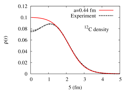
Figure 1: (Color online) Experimental point-proton density of ¹²C vries is compared to the symmetrized fermi function distribution with diffuseness $a$ = 0.44 fm and radius $R$ = 2.155 fm.

The diffuseness of the densities for both nuclei is set equal to 0.44 fm so the only parameters that need to be specified are the matter radii of the reacting nuclei. This choice of the diffuseness is in good agreement with the tail of the measured point-proton density of ¹²C vries which is illustrated in Fig. 1. The calculated point-proton distribution has the radius $R$ = 2.155 fm consistent with the measured rms charge radius. The radii that reproduce the point-proton (pp) rms radii of ¹²C and ¹³C, extracted from the measured root-mean-square (rms) charge radii angeli , are shown in the last few lines of Table I. The quoted radius for ¹²C is expected to be a realistic estimate of the matter radius of ¹²C and it will therefore be used in calculations of the M3Y double-folding potentials.

The matter radius of ¹³C is possibly larger than the radius of ¹²C because of the valence neutron. That is what one would expect by adding a neutron to an inert ¹²C core nucleus. A simple estimate based on a single-particle, Woods-Saxon potential gives a mean square radius of $\langle r^{2}_{n}\rangle$ = 8.655 fm² for the $p_{1/2}$ valence neutron. Combined with the point-proton rms radius of ¹²C, $\langle r^{2}\rangle_{12}$ = 5.462(9) fm², one can now estimate the mean square matter radius $\langle r^{2}\rangle_{13}$ of ¹³C by

$$13\langle r^{2}\rangle_{13}=12\Bigl{(}\langle r^{2}\rangle_{12}+\frac{\langle r^{2}_{n}\rangle}{13}\Bigr{)}.$$ (3)

The result is a rms matter radius of 2.378 fm. The associated radius of a fermi-function distribution with diffuseness $a$ = 0.44 fm is 2.228 fm according to the last line of Table I. This is a useful reference value for the discussion below.

A critical part of the M3Y+repulsion, double-folding potential is the repulsive part misi , which is generated by a contact interaction, $v_{r}\delta({\bf r})$. The densities that are used in calculating the repulsive, double-folding potential have the same radius as those that are used in the calculation of the M3Y double-folding potential but the diffuseness $a_{r}$ is chosen differently (usually smaller.) The strength $v_{r}$ of the repulsion, on the other hand, is adjusted for a given value of $a_{r}$ so that the nuclear incompressibility $K$ = 234 MeV is produced (see Ref. misi for details.) With this constraint there are three parameters that must be specified before the M3Y+repulsion potential can be calculated, namely, the matter radii of the two reacting nuclei, and the diffuseness parameter $a_{r}$ associated with the repulsion.

The parameters that give the best fit to Trentalange’s ¹³C+¹³C fusion data are the ¹³C radius $R$ = 2.28 fm and the diffuseness $a_{r}$ = 0.31 fm. How these parameters were determined is described in detail in section III.B. The radius $R$ = 2.28 fm is slightly larger than the 2.228 fm that was estimated from Eq. (3). That may not be unreasonable as discussed in Ref. 4848 because using a larger radius in a coupled-channels calculation is a way to compensate for the dynamic polarization of states that are not included explicitly in the calculation. The discrepancy between the estimated rms radius, Eq. (3), and the value extracted from the fit to the fusion data is only 1.2 %.

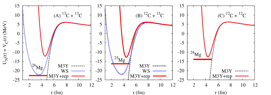
Figure 2: (Color online) The M3Y+repulsion double-folding potentials for different combinations of carbon isotopes. They are based on the parameter $a_{r}$ = 0.31 fm and the radius $R$ = 2.28 fm for ¹³C, and $R$=2.155 fm for ¹²C. The black dashed cures are the pure M3Y potentials. Also shown are the WS potentials discussed in the text and the ground state energies of the compound nuclei.

The entrance channel potential determined by the best fit parameters is shown by the solid curve in Fig. 2A. Also shown in Fig. 2 are the potentials that will be applied in calculating the fusion of ¹²C+¹³C and ¹²C+¹²C. They were obtained by setting the radius of ¹²C equal to the radius $R$ = 2.155 fm of the point-proton distribution of ¹²C (see Table I), and the diffuseness associated with the repulsion was set to $a_{r}$ = 0.31 fm.

The pure M3Y double-folding potentials shown in Fig. 2 are unphysical because they are much deeper for overlapping nuclei than the ground state energy of the compound nucleus. The (blue) dashed curve in Fig. 2A is the entrance channel potential for a standard Woods-Saxon (WS) potential with the depth $V_{0}$ = -39.31 MeV, radius $R_{ws}$ = 5.268 fm, and diffuseness $a$ = 0.63 fm. Here the radius was adjusted to optimize the fit to Trentalange’s fusion data as discussed in section III.A. This potential is deeper than the M3Y+repulsion potential and has a minimum that is close to the energy of the compound nucleus ²⁶Mg.

The three entrance channel potentials shown in Fig. 2A, which are based on the M3Y, the M3Y+repulsion and the Woods-Saxon potential, produce essentially the same Coulomb barrier height. $V_{CB}\approx$ 6 MeV. The most important features of the M3Y+repulsion potential are that it produces a shallow pocket and a relatively thick barrier. These features were utilized in Ref. misi to explain the hindrance of fusion that has been observed in the fusion of many medium mass systems at extreme subbarrier energies. The analysis of the ¹³C+¹³C fusion data discussed in the next section confirms that a shallow pocket in the entrance channel is a general feature that helps explain the energy dependence of fusion data.

II.2 Nuclear couplings

The nuclear couplings that excite the low-lying states of projectile and target are derived from the macroscopic description of surface excitations BW . In this description, the surface of nucleus $i$ is parametrized as

$$R_{i}({\hat{r}})=R_{i}^{(0)}\Bigl{(}1+\sum\alpha_{\lambda\mu}^{(i)}Y_{\lambda\mu}^{*}({\hat{r}})\Bigr{)},$$ (4)

where $\alpha_{\lambda\mu}^{(i)}$ are the (static or dynamic) deformation amplitudes of the nucleus, and ${\hat{r}}$ specifies a spatial direction. The distortion of the nuclear surface,

$$\delta R_{i}=R_{i}^{(0)}\sum\alpha_{\lambda\mu}^{(i)}Y_{\lambda\mu}^{*}({\hat{r}}),$$ (5)

is an operator that can excite and de-excite the nucleus (see chapter II.4 of Ref. BW .) The excitation can be vibrational, in which case the intrinsic hamiltonian is a harmonic oscillator, or it can be rotational, in which case $\alpha_{\lambda\mu}$ = $\beta_{\lambda}$ $D^{\lambda}_{\mu 0}({\hat{e}})$, where $\beta_{\lambda}$ is the static deformation parameter and ${\hat{e}}$ is the direction of the symmetry axis of the deformed nucleus.

In the macroscopic description of heavy-ion reactions BW , the nuclear potential between two colliding nuclei is parametrized in terms of the surface distortions $\delta R_{i}$ as follows

$$V_{N}(r-R_{1}^{(0)}-R_{2}^{(0)}-\delta R_{1}({\hat{r}})-\delta R_{2}(-{\hat{r}})),$$ (6)

where ${\hat{r}}$ is the direction of the center of mass distance between projectile and target. In the rotating frame approximation, which is a simplifications that is commonly used and which will be used in coupled-channels calculations, the direction of ${\hat{r}}$ defines the z-axis, so that

$$\delta R_{1}({\hat{r}})=R_{1}^{(0)}\sum_{\lambda}\alpha_{\lambda 0}^{(1)}\ \sqrt{\frac{2\lambda+1}{4\pi}}.$$ (7)

In the model of heavy-ion fusion reactions described in Ref. alge , the nuclear potential is expanded up to second order in the surface distortions,

$$U_{N}(r,\delta R_{1},\delta R_{2})=V_{N}-\frac{dV_{N}}{dr}(\delta R_{1}+\delta R_{2})$$

$$+\frac{1}{2}\ \frac{d^{2}V_{N}}{dr^{2}}\ \Bigl{[}(\delta R_{1}+\delta R_{2})^{2}-\langle 0|(\delta R_{1}+\delta R_{2})^{2}|0\rangle\Bigr{]},$$ (8)

where the argument of $V_{N}$ and its derivatives is $r-R_{1}^{(0)}-R_{2}^{(0)}$. The second-order term in this expression has been renormalized so that the ground state expectation value of that term is zero. The ground state expectation value of the first-order term (proportional to $\delta R_{1}$+$\delta R_{2}$) will also vanish if the ground states of the two reacting nuclei are $0^{+}$ states. The ground state expectation of the entire expression, Eq. (8), is therefore identical to the ‘bare’ interaction, i. e.,

$$\langle 0|U_{N}(r,\delta R_{1},\delta R_{2})|0\rangle=V_{N}(r-R_{1}^{(0)}-R_{2}^{(0)}).$$ (9)

This implies that the M3Y+repulsion potential which is calculated using the ground state densities of the reacting nuclei can be used as the bare interaction, $V_{N}$.

The diagonal matrix element of the first-order term in Eq. (8) can be non-zero, for example, in the $2^{+}$ state of a deformed nucleus. The calculation of diagonal and off-diagonal matrix elements is outlined in the appendix. Details of how to calculate the matrix elements of the second-order couplings in Eq. (8), both for vibrational and rotational excitations, are given in Ref. alge .

II.3 Nuclear structure input

The nuclear structure input to the coupled-channels calculations is listed in Table II. The nuclei ¹²C and ¹³C are both considered deformed with oblate quadrupole shapes. The connection between the deformation parameter $\beta_{\lambda}$ and the measured $B(E2)$ values is summarized in the appendix. For ¹²C one can extract the quadrupole deformation parameter $\beta_{2}$ = 0.57(2) from the measured strength of the $0_{1}^{+}\rightarrow 2^{+}$ transition. The value of this deformation parameter produces an intrinsic quadrupole moment of $Q_{0}$ = -19.5 fm² (assuming an oblate shape). The quadrupole moment of the $2^{+}$ state is therefore $Q_{2}$ = -2/7$Q_{0}$ = 5.57 fm², which is consistent with the measured value of $6\pm 3$ fm² vermeer . Also shown in the Table is the structure information about the $2^{+}\rightarrow 0_{2}^{+}$ transition which is included in the calculations as part of the two-phonon quadrupole excitation of ¹²C.

Values of quadrupole deformation parameter $\beta_{2}$ of ¹³C, extracted from Eq. (21) of the appendix and the known strengths of the quadrupole transition from the 1/2^- ground to the 3/2^- and the 5/2^- excited states, are shown in the last column of Table II. They are seen to be almost identical, which indicates that ¹³C is a fairly good rotor. Assuming the deformation parameter $\beta_{2}$ = 0.495 and an oblate shape, one obtains the intrinsic quadrupole moment $Q_{0}$ = -17.9 fm².

The strength of the octupole transition in ¹³C quoted in Table II appears to be very large and almost as large as the octupole strength in ¹²C. This is misleading because what matters is the off-diagonal matrix element of the octupole amplitude, which is given by Eq. (19) of the appendix. In ¹²C the matrix element is

$$\langle 300|\alpha_{30}|000\rangle=\frac{\beta_{3}}{\sqrt{7}},$$ (10)

whereas in ¹³C it is (with $M$ = $K$= 1/2)

$$\langle{\frac{5}{2}\ \frac{1}{2}\ \frac{1}{2}}|\alpha_{30}|\frac{1}{2}\ \frac{1}{2}\ \frac{1}{2}\rangle=\beta_{3}\sqrt{\frac{2}{6}}\ \langle\frac{1}{2}\frac{1}{2}\ 30|\frac{5}{2}\frac{1}{2}\rangle^{2}=\sqrt{\frac{3}{7}}\ \frac{\beta_{3}}{\sqrt{7}}.$$ (11)

The matrix element of the octupole amplitude is therefore reduced in ¹³C by the factor $\sqrt{3/7}\approx$ 0.655 relative to the expression Eq. (10) for ¹²C.

The coupled-channels calculations that are performed are similar to those presented in Ref. alge for the fusion of ²⁷Al with different germanium isotopes. In addition to the nuclear couplings derived from the nuclear interaction, Eq. (8), the Coulomb interaction (Eq. (2) of Ref. alge ) is included in the calculations to first order in the deformation amplitudes.

II.4 Transfer reactions

The one-neutron transfer reactions that will be considered all involve the $p_{1/2}$ orbit, both in the initial and final states. One example is the ground state to ground state transfer reaction, ¹²C(¹³C,¹²C)¹³C, which has zero Q value. The spectroscopic factors for the initial and final state $1/2^{-}$ state in ¹³C were set equal to 0.75(10), which is the value recommended in Table III of Ref. jenny .

The other example is the one-neutron transfer from ¹³C+¹³C to the ground states of ¹²C+¹⁴C which has a Q-value of +3.2 MeV. The spectroscopic factor for the initial state is the same as above. It is set equal to 2*0.75 in the calculations because the transfer can take place from either of the two ¹³C nuclei in the entrance channel. The spectroscopic factor for the $p_{1/2}$ orbit in the $0^{+}$ ground state of ¹⁴C is 1.63(33) according to table III of Ref. jenny .

The transfer form factors that are used are the so-called Quesada single-particle form factors quesada which in the past turned out to be fairly realistic opb ; NPA492 . They have here been calibrated against calculations performed with the computer code Ptolemy ptol of the one-neutron transfer cross in ¹²C+¹³C collisions at a 5.2 MeV center-of-mass energy.

II.5 Calculation of fusion cross sections

The fusion cross section is calculated from the ingoing flux which is determined by the ingoing-wave-boundary conditions (IWBC) that are imposed at the minimum of the pocket in the entrance channel potential. This approximation ignores the internal structure of the combined di-nuclear or compound system and the calculated cross sections are usually fairly smooth functions of energies, at least at energies near and below the Coulomb barrier.

At energies far above the Coulomb barrier, there are sometimes numerical problems in the coupled-channels calculations which can cause an erratic behavior of the calculated cross section as a function of energy. One can overcome these problems by applying a weak imaginary potential misi

$$W(r)=\frac{W_{0}}{1+\exp((r-R_{\rm w})/a_{\rm w})},$$ (12)

which acts near the position $R_{\rm w}$ of the pocket in the entrance channel potential. The fusion cross section is then defined as the sum of the absorption cross section and the cross section for the ingoing flux. A weak imaginary potential will be applied in the following when the calculated fusion cross section is shown in a linear plot at energies far above the Coulomb barrier. The parameters that are used are $W_{0}$ = -5 MeV and $a_{\rm w}$ = 0.5 fm. No imaginary potential will be used in the calculations at energies below the Coulomb barrier.

The 1/2^- ground state spin of ¹³C causes some concern when calculating the scattering and fusion of ¹³C+¹³C. The fermionic nature of ¹³C requires that the total wave function for ¹³C+¹³C be anti-symmetric. By coupling the intrinsic $1/2^{-}$ ground state spins of the reacting nuclei one obtains a total spin of $S$=0 (anti-symmetric) and $S$=1 (symmetric). The wave function for the relative motion of the two nuclei must therefore be symmetric for $S$=0, i. e., it consists of even partial waves, and it must be antisymmetric for $S$=1, consisting of odd partial waves. The fusion cross section is therefore calculated as the weighted sum

$$\sigma_{f}=\frac{1}{2}\ \sigma({\rm even}\ L)+\frac{3}{2}\ \sigma({\rm odd}\ L).$$ (13)

It turns out that the contributions to the fusion cross section from odd and even $L$-values are almost identical. The biased weighting of the two contributions in Eq. (13) does therefore not have much effect. In calculations of the fusion and elastic scattering of two identical spin zero ¹²C nuclei, one should only consider the contribution from even partial waves which is doubled because of the symmetry of two identical particles. In reactions of ¹²C+¹³C, on the other hand, the contribution from even and odd partial waves have the same weight.

III Analysis of the ¹³C+¹³C fusion data

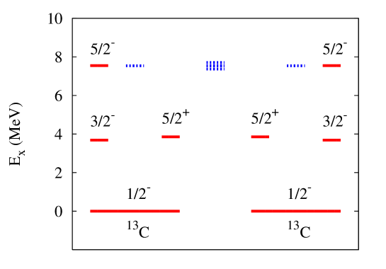
Figure 3: (Color online) Excitation energies of the channels considered in the calculations of the fusion of ¹³C+¹³C. The (red) solid lines are the excitations in projectile and target of the ¹³C states shown in Table I. The (blue) dashed lines are the 6 mutual excitations that involve the 3/2^- and 5/2⁺ states in projectile and target.

In this section the ¹³C+¹³C fusion data by Trentalange et al. trent and Charvet et al. char are analyzed in terms of coupled-channels calculations. The channels that are included are enumerated in Fig. 3. The (red) solid lines represent the elastic channel and the channels associated with the excitation of the states shown in Table II, in both projectile or target. The calculation based on these channels is referred to as the one-phonon (ph1) calculation and has a total of 7 channels.

The (blue) dashed lines in Fig. 3 are the 6 mutual excitations of the lowest quadrupole and octupole excitations in projectile and target. These include the four mutual states $(I_{1},I_{2})$, where $I_{i}$ = $3/2^{-}$ or $5/2^{+}$, $i$=1,2, and $I_{1}$ and $I_{2}$ belong to different nuclei, and the two $(3/2^{-},5/2^{+})$ mutual excitations that belong to the same nucleus. Together with the seven channels of the one-phonon calculation that gives a total of 13 channels. This calculation is referred to as the mutual excitation calculation or Ch13.

The calculation Ch13 will be compared to the one-phonon calculation (ph1) described above and the no-coupling limit which has only one channel. There are other excitations, for example, the two-phonon excitations which are poorly known and mutual excitations that involve the $5/2^{-}$ state but they are all ignored in the following.

It can be very difficult to see small discrepancies between measured and calculated cross sections, in particular, when they are plotted on a conventional logarithmic scale. It is therefore useful to use other representations that amplify certain features of the comparison, such as the $S$ factor for fusion, which emphasizes the behavior at low energies. Another representation, which is very useful when coupled-channels effects are modest, is the so-called enhancement factor, which was used in the early days when the enhancement of subbarrier fusion was first discovered. It is defined as the ratio of a cross section relative to the cross section calculated in the no-coupling limit, and it will be used both for measurements as well as coupled-channels calculations, as long as it is indicated which no-coupling limit is used as a reference. Finally, the comparison of data and coupled-channels calculations will also be made in terms of the ratio of the measured and calculated cross sections. If the measured and calculated cross sections agree, the ratio should be close to one.

The one-neutron transfer discussed earlier is included as an independent degree of freedom. That implies that the transfer can take place from any excited state and it is calculated with the same form factor which describes the ground state to ground state transition. The full calculation (with 13 excitation channels mentioned above and the one-neutron transfer) will therefore contain 26 channels and is referred to as the Ch26 calculation.

The analysis of the data is performed in terms of the $\chi^{2}$ per data point, $\chi^{2}/N$, which is minimized by adjusting certain parameters of the ion-ion potential. The overall normalization of the calculated cross sections is also adjusted by a multiplicative factor $S_{c}$, in order to improve the fit to the data. The motivation for this adjustment is the large uncertainty in the absolute normalization of the measured cross sections that was mentioned in the introduction. The shape (i.e., the energy-dependence) of the measured cross section is assumed to be more accurately determined. The uncertainty in the data analysis will therefore include the statistical uncertainty and an adopted systematic error of only 3%, which is much smaller than the 15% experimental error trent .

III.1 Application of Woods-Saxon potential

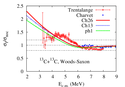
Figure 4: (Color online) Enhancement of the fusion of ¹³C+¹³C relative to the cross section of the no-coupling calculation. Shown are the enhancement of the one-phonon calculation (ph1), the mutual excitation (Ch13) calculation, and the full calculation (Ch26) which also includes one-neutron transfer. The calculations are based on a standard Woods-Saxon potential with radius $R_{ws}$ = 5.268 fm. Also shown are the ratios of the measured cross sections trent ; char relative to the no-coupling limit.

The first set of calculations are based on a standard Woods-Saxon potential with typical parameters from Ref. BW . The diffuseness of the potential is set to $a$ = 0.63 fm and the depth is -39.31 MeV. The radius of the potential, $R_{ws}$ = 5.268 fm, was adjusted to optimize the fit to the data of Ref. trent . A comparison to the data is made in Fig. 4 in terms of the enhancement of the cross sections with respect to the no-coupling limit. The enhancement of the measured cross sections is seen to deviate from the enhancement of the coupled-channels calculation (Ch26) by up to 20%. Moreover, the effects of mutual excitations and one-neutron transfer are seen to be modest by comparing to the no-transfer calculations (Ch13) and the one-phonon calculations (ph1). It is very unlikely that the agreement with the data can be improved much by adjusting the strengths of the couplings to the excitation or transfer channels. It is shown in the next subsection that a much better agreement with the data is achieved by applying the M3Y+repulsion instead of the Woods-Saxon potential.

The agreement with the data in Fig. 4 cannot be improved much by scaling the calculated cross sections with an adjustable scaling factor $S_{c}$ in the data analysis. The best fit for $S_{c}$ = 1 has a $\chi^{2}/N$ = 8.7. It can be reduced to $\chi^{2}/N$ = 6.8 by adjusting both the scaling factor $S_{c}$ and the radius $R_{ws}$ of the Woods-Saxon well. The values that give the best fit are $S_{c}$ = 0.885 and $R_{ws}$ = 5.345 fm.

Another observation in Fig. 4 is that the data sets of Trentalange et al. trent and Charvet et al. char differ by up to 10% in the overlapping energy regime. However, this is not a serious problem because the systematic error of both experiments is about 15%.

III.2 Application of the M3Y+repulsion potential

One advantage of the M3Y+repulsion potential is that it has an additional adjustable parameter besides the radius $R$ of the density, namely, the diffuseness parameter $a_{r}$ of the density that is used in calculating the repulsive part of the potential. This parameter controls the depth of the pocket and the thickness of the barrier in the entrance channel potential.

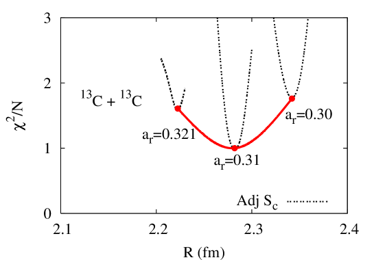
Figure 5: (Color online) Results of the $\chi^{2}$ analysis of the ¹³C+¹³C fusion data trent as function of the radius of ¹³C. The dashed curves show the $\chi^{2}/N$ for the indicated fixed values of $a_{r}$ and minimized with respect to the scaling factor $S_{c}$. The parameters of the best solution for $a_{r}$ = 0.31 fm are shown in Table 1.

The determination of the best fit parameters is illustrated in Fig. 5. For a fixed value of $a_{r}$, the fusion cross sections were calculated for different values of the radius $R$ of ¹³C. In each case the scaling factor $S_{c}$ was adjusted to give the best $\chi^{2}/N$. The results are shown by the dashed curves. The minimum $\chi^{2}/N$ for each dashed curve defines the solid curve, and the minimum of this curve defines the absolute best fit (ABF) to the data. The parameters of the minimum are $a_{r}$ = 0.31 fm, the matter radius $R$ = 2.28 fm, and the scaling factor $S_{c}$ = 0.843. They are compared in Table 1 to other parameters that were obtained for fixed choices of the radius of ¹³C.

The $\chi^{2}/N$ of the best fit to Trentalange’s data is small according to Table 1, $\chi^{2}/N$ =1.0, although the adopted systematic error of the analysis was set to only 3%. The scaling factor of the best fit, $S_{c}$ = 0.843, is not unreasonable but it is slightly extreme because the systematic uncertainty in the absolute cross section of the measurement was estimated to be 15% trent . It is therefore of interest to discuss whether the other parameters of the best fit are realistic. The diffuseness $a_{r}$ associated with the repulsion, $a_{r}$ = 0.31 fm, falls below the range of values $a_{r}$ = 0.4 – 0.43 fm that have been obtained in the analysis of fusion data for other symmetric heavy-ion systems 4848 .

The ¹³C radius of the best fit, $R$ = 2.28 fm, produces an rms matter radius of 2.407 fm according to Table 1 which is slightly larger than the rms matter radius of 2.378 fm that was estimated in Eq. (3). This result is not unreasonable as discussed in connection with an analysis of the fusion data for ⁴⁸Ca+⁴⁸Ca 4848 . There it was pointed out that a larger radius may simulate the effect of the dynamic polarization of excited states which are not included explicitly in the coupled-channels calculations.

If the scaling parameter $S_{c}$ is kept fixed at $S_{c}$=1 in the data analysis, the best fit is achieved with a smaller ¹³C radius, namely, $R$ = 2.17 fm. This value is almost as small as the radius for the point-proton density distribution of ¹³C. The fit is poor, with a $\chi^{2}/N$ = 2.75 as shown in the first line of Table I. The value of the diffuseness parameter $a_{r}$ which produces the best fit in this case is $a_{r}$ = 0.33.

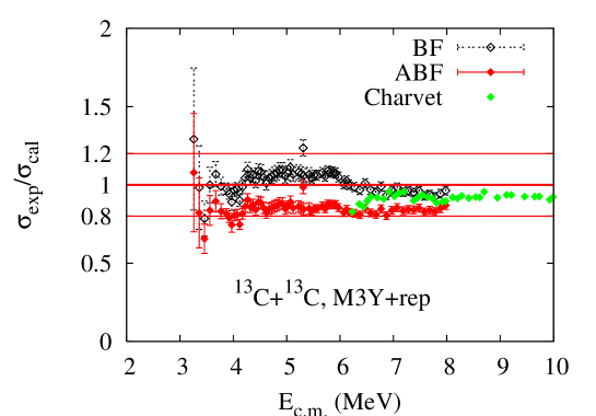
Figure 6: (Color online) Ratios of the measured trent and calculated fusion cross sections for ¹³C+¹³C. The coupled-channels calculations include 26 channels and are based on the M3Y+repulsion potential using the ¹³C radius $R$ = 2.17 fm (BF, $S_{c}$=1) and $R$=2.28 fm (ABF, $S_{c}$=0.843), respectively. Also shown is the ratio of Charvet’s data char and the calculation that uses the radius $R$ = 2.28 fm.

The ratios of the measured and calculated cross sections discussed above are illustrated in Fig. 6. The ratio of Trentalange’s data trent to the best fit (BF) solution with radius $R$ = 2.17 and $S_{c}$ = 1 is shown by the open symbols. The ratio of the same data set to the absolute best solution (ABF) with radius $R$ = 2.28 fm is shown by the solid (red) points. Also shown at higher energies is the ratio of Charvet’s data char to the same solution (with radius $R$ = 2.28 fm.) It is seen that the ratios for the absolute best solution are essentially constants ($\approx$ 0.84 for Trentalange’s data, and $\approx$ 0.92 for Chatvet’s data up to 10 MeV). The two data sets differ by up to 10% in the overlapping energy regime. However, this is not a serious problem as mentioned earlier because the systematic error of both experiments is about 15%.

The ratio for best fit (BF) solution for $S_{c}$=1 exhibits some energy dependence in Fig. 6. It is of course possible that the data do contain some structures (similar to those observed in the ¹²C+¹²C fusion data) that should not be accounted for by the type of coupled-channels calculations performed here. The absolute best fit (ABF) solution, obtained with the ¹³C radius $R$ = 2.28 fm and $S_{c}$ = 0.843, could therefore be misguided or misleading. On the other hand, the absolute best fit does have some attractive features as argued above: the quality of the fit is excellent, and the extracted rms matter radius is only 1.2% larger than expected. The absolute best fit requires a scaling of the calculation, $S_{c}$ = 0.843, which is not unreasonable considering the large 15% systematic error of the experiment. The parameters of the ABF are therefore adopted in the following.

III.3 Results of the analysis

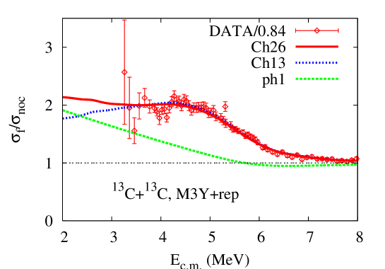
Figure 7: (Color online) Enhancement of the fusion of ¹³C+¹³C trent relative to the cross sections obtained in the no-coupling limit. The curves show the enhancement of calculations that include one-phonon (ph1) and mutual excitations (Ch13), and the full calculation (Ch26) which also includes one-neutron transfer. The enhancement factors for Trentalange’s data trent have been divided by the optimum scaling factor, $S_{c}$ = 0.843.

In order to illustrate what makes it possible to reproduce the energy dependence of Trentalange’s data so well when using the M3Y+repulsion potential, we show in Fig. 7 the enhancement of the calculations and the data relative to the no-coupling calculation. In contrast to the results for the Woods-Saxon potential shown in Fig. 4, there is now a strong sensitivity to mutual excitations. This is caused by a larger second derivative of the ion-ion potential (stemming from the onset of the strong repulsion), and consequently, a stronger quadratic coupling of the entrance channel to mutual excitations.

An interesting observation in Fig. 7 is that the neutron transfer does not have much influence on the calculated cross section in the energy regime of the experiment. This is seen by comparing the calculations labeled Ch13 and Ch26. The influence shows up at energies below 3 MeV, so it will have an impact on the extrapolation of the cross sections to lower energies. Another interesting feature in Fig. 7 is the structure of the data at low energies. The small peaks at 3.6 and 4.2 MeV, for example, could be remnants of similar structures observed in the fusion data for ¹²C+¹²C.

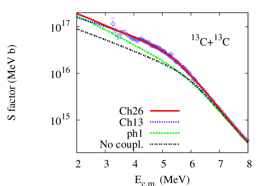
Figure 8: (Color online) $S$ factors for the fusion of ¹³C+¹³C calculated using the M3Y+repulsion potential. They are compared to the data of Ref. trent , which have been divided by the scaling factor $S_{c}$ = 0.843.

The calculated $S$ factors for the fusion of ¹³C+¹³C are compared in Fig. 8 to the data of Ref. trent . The data have here been divided by the scaling factor $S_{c}$ = 0.843 which optimizes the agreement with the full calculation labeled Ch26. The calculation that is based on one-phonon excitations only (ph1) does no reproduce the energy dependence of the data between 3 and 6 MeV. The calculation that includes mutual excitations but no transfer (the Ch13 calculation) is seen to reproduce the corrected data very well. Finally, the additional coupling to the one-neutron transfer produces some enhancement in the full Ch26 calculation but that occurs at energies below the range of the experiment.

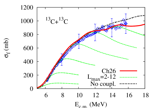
Figure 9: (Color online) Measured fusion cross sections for ¹³C+¹³C char are compared to the full coupled-channels calculation (Ch26, the solid curve). The thin (green) dashed curves are the calculated cross sections for a maximum angular momentum of $L_{max}$ = 2, 4, 6, 8, 10 and 12. The (black) dashed curve shows the no-coupling limit.

The calculated cross sections obtained with all 26 coupled channels and the parameters determined in the previous subsection are compared in Fig. 9 to the data of Ref. char . The calculation exceeds the data on average by only 4%, which is small compared to the 15% systematic error of the experiment. The coupled-channels effects are fairly modest at high energies; this can be seen by comparing to the no-coupling calculation which is shown by the thick dashed curve. The results of a maximum angular momentum cutoff in the coupled-channels calculations are shown for $L_{max}$ = 2 - 12.

IV Predictions of the fusion of ¹²C+¹³C

Having determined the radius of ¹³C and the diffuseness $a_{r}$ associated with the repulsive part of the double-folding potential in the previous section, one can now predict the ion-ion potential for ¹²C+¹³C, provided the density of ¹²C is known. Here the parameters of the point-proton density of ¹²C given in Table 1 are adopted. The predicted M3Y+repulsion potential is shown in Fig. 2B. It is similar to ¹³C+¹³C potential shown in Fig. 2A. The main difference between the two figures is that the ground state of the compound nucleus ²⁵Mg is located at a higher energy than ²⁶Mg because of the unpaired neutron in ²⁵Mg.

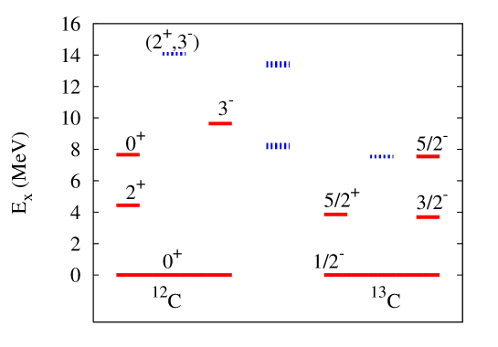
Figure 10: (Color online) Excitation energies of the channels considered in the calculations of the ¹²C+¹³C fusion cross section. The (red) solid lines are the states given in Table I. The blue lines are mutual excitations considered in the calculations.

The excitation energies that are considered in the calculations of the fusion cross sections for ¹²C+¹³C are shown in Fig. 10. The solid (red) lines represent the excitations shown in Table I which together with the elastic channel give a total of 7 channels. One of these states is the $0_{2}^{+}$ Hoyle state of ¹²C which is included because its coupling to the $2^{+}$ is known.

The (blue) dashed lines in Fig. 10 are the 6 mutual excitations that are considered. They include the $(2^{+},3^{-})$ mutual excitation in ¹²C, the $(3/2^{-},5/2^{+})$ mutual excitation in ¹³C, and the four $(I_{1},I_{2})$ mutual excitations in projectile and target with $I_{1}$ = $2^{+}$ or $3^{-}$ and $I_{2}$ = $3/2^{-}$ or $5/2^{+}$. Two-phonon excitations (except the $0_{2}^{+}$ Hoyle state which has already been mentioned) and mutual excitations that involve the $5/2^{-}$ state in ¹³C are ignored. The total number of excitation channels is therefore 7+6 = 13. When the one-neutron transfer with zero Q value is included in the calculations as described in Sect. II.D, the number of channels is doubled. The full calculation, which includes the one-neutron transfer and all of the 13 excitation channels shown in Fig. 10 will therefore have 26 channels and it is referred to as Ch26.

A major problem, which causes some uncertainty in the predictions made by the coupled-channels calculations, is the high excitation energy and the large strength of the octupole transition in ¹²C (see Table 1.) A large excitation energy implies decaying boundary conditions at large separations of projectile and target instead of the scattering boundary conditions, and this can cause numerical problems. A large octupole strength implies a strong sensitivity to mutual excitations that involve the $3^{-}$ state and some of these excitations are poorly known as explained below. The octupole excitation of ¹³C, on the other hand, is not a problem because the excitation energy of the $5/2^{+}$ state is much lower than in ¹²C, and the effective octupole strength is reduced as shown in Eq. (11).

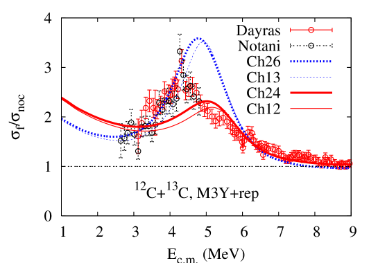
Figure 11: (Color online) Enhancement factors of the measured ¹²C+¹³C fusion cross sections dayras ; tang1 relative to the cross sections obtained in the no-coupling limit. The curves show the enhancement of calculations that include the 24 (Ch24) and 26 (Ch26) channels described in the text. The associated calculations without transfer, Ch12 and Ch13, are shown by the thin curves.

The enhancement of the ¹²C+¹³C fusion relative to the no-coupling limit is shown in Fig. 11 for different coupled-channels calculations. The full calculation Ch26 has a very strong peak near 4.7 MeV. The calculation Ch24, which excludes the mutual $(2^{+},3^{-})$ excitation in ¹²C, has a much weaker peak. There are two reasons why the mutual $(2^{+},3^{-})$ excitation in ¹²C has such a large influence on subbarrier fusion. One reason is the large octupole strength of ¹²C. The other reason is that the direct coupling of the ground state to mutual excitations is governed by the second derivative of the ion-ion potential, according to Eq. (8), and this quantity is particularly large for the M3Y+repulsion potential as pointed out in section III.C.

It is very interesting that the enhancement of the data dayras ; tang1 with respect to the no-coupling limit also exhibits a peak structure in Fig. 11. The peak is located near 4.3 MeV, somewhat below the positions of the two calculated peaks. The influence of transfer can be seen by comparing the thin curves C12 and Ch13, which do not include the influence of transfer, to the corresponding thick curves Ch24 and Ch26, which include the effect. The influence is relatively modest but it does shift the calculated peaks towards the peak position of the data.

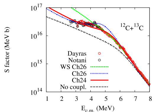
Figure 12: (Color online) $S$ factors for the fusion of ¹²C+¹³C dayras ; tang1 are compared to calculations that are based on a Woods-Saxon potential and 26 channels (WS Ch26), and on the M3Y+repulsion potential with 24 and 26 channels, respectively. The no-coupling limit is also shown.

The $S$ factor for the fusion of ¹²C+¹³C is illustrated in Fig. 12. The calculation ‘WS Ch26’ is based on the standard Woods-Saxon potential with radius $R_{ws}$ = 5.352 fm, depth $V_{0}$ = -38.6 MeV, and diffuseness $a$ = 0.63 fm, which was illustrated in Fig. 2B. It includes all 26 channels considered in this sections and makes a very good fit to the data above 4 MeV. However, a strong hindrance of the data sets in at energies below 4 MeV. The comparison shows that the fusion of ¹²C+¹³C is an example on the fusion hindrance phenomenon which has been observed in many medium heavy systems niy ; sys .

The two calculations Ch24 and Ch26 that are based on the M3Y+repulsion potential reproduce the data in Fig. 12 at the lowest and also at high energies. The calculation Ch26 exceeds the data between 4.5 and 5.5 MeV by up to 50%. The calculation Ch24 is in better agreement with the data but there are still some deviations. The measured $S$ factor is rather flat between 3 and 4 MeV and has a modest peak near 4.3 MeV. The calculated $S$ factors do not exhibit any sharp peak structures but rise slowly with decreasing energy.

The two calculations Ch24 and Ch26 represent extreme views of the influence of the mutual excitation of the $2^{+}$ and $3^{-}$ states in ¹²C, i. e., of a quadrupole excitation built on the $3^{-}$ state or an octupole excitation built on the $2^{+}$ state. The calculation Ch24 completely ignores it, whereas the calculation Ch26 exaggerates it by assuming that the $2^{+}$ and $3^{-}$ excitations are independent modes of excitation. In a realistic, microscopic description, the mutual excitation of the $2^{+}$ and $3^{-}$ states will not be one discrete excitation but will be fragmented and spread out over a range of excitation energies. This is indeed the result of shell model calculations that are discussed in section VI.

V Predictions of the fusion of ¹²C+¹²C

Similar predictions are made for the fusion of ¹²C+¹²C. The entrance channel potential that is used is shown in Fig. 2C. It was obtained with the parameters of the point-proton density of ¹²C shown in Table I, and the diffuseness associated with the repulsive part of the M3Y+repulsion interaction was again set equal to the value $a_{r}$ = 0.31 fm which was determined in the analysis of the ¹³C+¹³C fusion data.

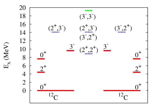
Figure 13: (Color online) Excitation energies of the channels considered in the calculations of the ¹²C+¹²C fusion cross section. The (red) solid lines are the states given in Table I. The (blue) dashed lines are the mutual excitations considered in the calculations. The $(3^{-},3^{-})$ mutual excitation of projectile and target is indicated but it is ignored in the calculations.

The excitation energies that are considered in the coupled-channels calculations are shown in Fig. 13. The solid (red) lines represent the excitations shown in Table I which together with the elastic channel give a total of 7 channels. The second $0^{+}$ state is Hoyle state. The (blue) dashed lines in Fig. 13 are the mutual excitations that are considered in the calculations. They include the three mutual excitations: $(2^{+},2^{+})$, $(2^{+},3^{-})$ and $(3^{-},2^{+})$, with a one-phonon excitation in each ¹²C nucleus, and the two mutual excitations: $(2^{+},3^{-})$, with both one-phonon excitations belonging to the same nucleus. There is also a $(3^{-},3^{-})$ mutual excitation indicated in the figure (with one octupole excitation in each nucleus) but it is ignored because the excitation energy is very high. The total number of channels consisting of the 7 channels mentioned above (represented by the solid (red) lines in Fig. 13) and the 5 mutual excitation channels (the (blue) dashed lines in Fig. 13) is therefore 12. The associated coupled-channels calculation is referred to as Ch12.

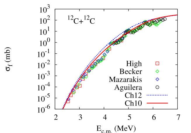
Figure 14: (Color online) Measured fusion cross sections for ¹²C+¹²C aguilera ; becker ; high ; maza are compared to the Ch10 and Ch12 coupled-channels calculations discussed in the text. The data of Refs. maza ; high have been shifted in energy ($\Delta E$ = +100 keV maza and $\Delta E$ = +75 keV high , respectively) following the suggestions of Ref. aguilera .

The calculation Ch12 includes the mutual excitation of the $2^{+}$ and $3^{-}$ states, not only when the two states belong to different nuclei but also when they belong to the same nucleus. Since the description of the $(2^{+},3^{-})$ mutual excitation in terms of two independent modes of excitation is questionable when the two excitations belong to the same nucleus, it is of interest to perform a calculation that does not include that kind of mutual excitation. Such a calculation contains 10 channels and is referred to as Ch10. The Ch10 calculation does contain mutual excitations of the $2^{+}$ and $3^{-}$ states but only when the two one-phonon excitations belong to different nuclei. The two calculations are compared in Fig. 14 to the measured cross sections of Ref. maza ; high ; aguilera ; becker . The Ch12 calculation exceeds the data substantially between 3 and 5.5 MeV, whereas the Ch10 calculation is lower and intersects with some of the measured peak cross sections.

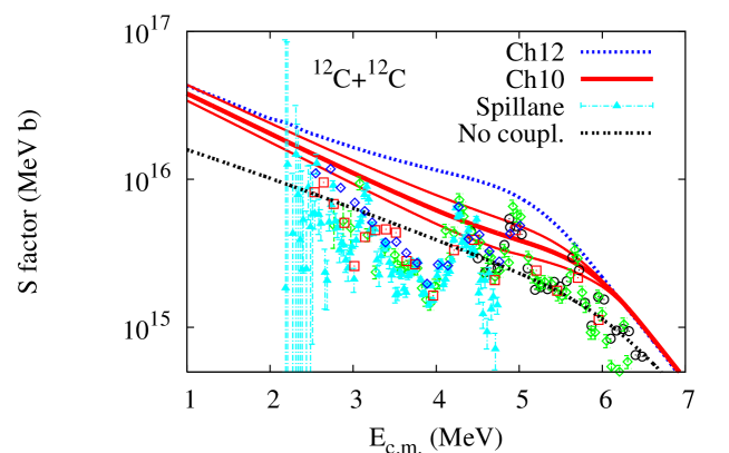
Figure 15: (Color online) Measured $S$ factors for the fusion of ¹²C+¹²C aguilera ; high ; maza ; becker ; spillane are compared to the coupled-channels calculations Ch10 and Ch12, and to the no-coupling limit. The thin solid curves show the error band in Ch10 calculations due to the uncertainty in the octupole strength, $\beta_{3}$ = 0.90 $\pm$ 0.07.

The $S$ factors for the fusion of ¹²C+¹²C predicted by the Ch10 and Ch12 calculations are compared in Fig. 15 to the data of five experiments maza ; high ; aguilera ; becker ; spillane . The symbols for the four measurements maza ; high ; aguilera ; becker are the same as in Fig. 14, whereas the symbol for Spillane’s measurements spillane is indicated in the figure. The calculation Ch12 exceeds all of the data points shown in this figure. It is considered an extreme upper limit because it exaggerates, as discussed above and in the previous section, the influence of the mutual $(2^{+},3^{-})$ excitation within the same nucleus. The calculation Ch10, which is much lower, is considered a lower limit of the prediction.

The large difference between the Ch10 and Ch12 calculations shown in Fig. 15 is very unfortunate. It illustrates the difficulty and uncertainty in predicting the fusion cross section due to the poor empirical knowledge of excitations that are built on the $2^{+}$ and $3^{-}$ states. We shall eliminate that problem in the next section by applying the results of shell model calculations. Another uncertainty, which is similar in magnitude, is due to the empirical value $\beta_{3}$ = 0.90(7) ENDSF . This is illustrated in the figure by the thin lines and represents an error band of up to $\pm$25%.

The $S$ factor one obtains in the no-coupling limit is shown by the lowest dashed curve in Fig. 15. It is a factor of 2 to 3 below the measured peak cross sections and a factor of 2 to 5 above the minima of the measured cross sections. In other words, it does not provide a background nor does it provide an upper limit of the measured cross sections. It is closer to the smooth experimental cross section constructed by Yakovlev et al. yakovlev .

VI Systematics of the fusion of carbon isotopes

The discussion in the previous sections shows that it is possible to develop a fairly comprehensive description of the fusion data for the three carbon systems within the coupled-channels approach. A disturbing trend in the analysis of the ¹³C+¹³C fusion data trent is the need for dividing the data by the factor $S_{c}$ = 0.843, i. e., for increasing the measured cross sections by 19%. However, that is not a very serious problem because the systematic error of the experiment trent is 15%.

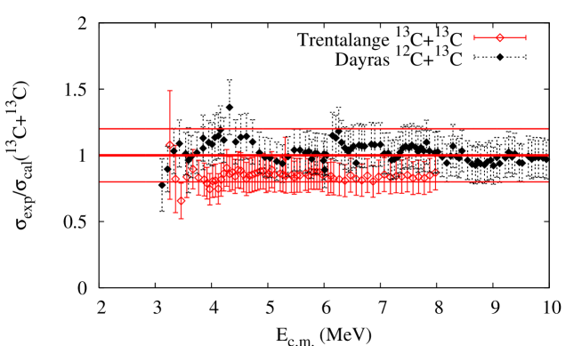
Figure 16: (Color online) Ratios of measured fusion cross sections relative to the calculation Ch26 of the fusion of ¹³C+¹³C. The error bars include a 15% systematic error. The average ratio for the ¹²C+¹³C data dayras is 1.02, whereas the average ratio for the ¹³C+¹³C data trent is 0.843.

The need for a renormalization of the ¹³C+¹³C data is possibly an experimental problem because it is difficult to explain why the measured fusion cross sections for ¹²C+¹³C dayras are larger than the measured cross sections for ¹³C+¹³C trent . Naively, one would expect the cross sections for the smaller system to be smaller. This is indeed the ordering that is observed in the fusion of carbon isotopes with a thorium target alcorta . Of course, the problem could be in the absolute normalization of ¹²C+¹³C data dayras . Whatever the explanation is, the basic problem is illustrated in Fig. 16, where the measured cross sections for the two systems have both been normalized to the Ch26 calculation for the ¹³C+¹³C system discussed in sections III.B. It is seen that the normalized cross sections are fairly constant but the cross sections for the smaller ¹²C+¹³C system are larger, on average by the factor 1.02/0.84 = 1.21 (c. f. the caption to Fig. 16). The 21% deviation between the two measurements is within the large uncertainties of the two experiments, each being of the order of 15 to 30% but it does show an unexpected trend. Clearly, it is desirable to have the experimental uncertainties reduced in future measurements.

Another disturbing feature discussed in the previous section is the large uncertainty in the cross section predicted for the fusion of ¹²C+¹²C. Half of the uncertainty concerns the influence of the $(2^{+},3^{-})$ mutual excitation which is poorly known experimentally ENDSF . One way to overcome this problem is to rely on shell model calculations brown which predict that E2 excitations built on the $3^{-}$ state and E3 excitations built on the $2^{+}$ state primarily populate a $4^{-}$ state which is about 4 MeV above the $3^{-}$ state. That is similar to the model we have used for the mutual $(2^{+},3^{-})$ excitation. However, the B-values of these transitions are only about half of the B-values obtained for the corresponding E2 and E3 transitions from the ground state to the first $2^{+}$ and $3^{-}$ states in ¹²C.

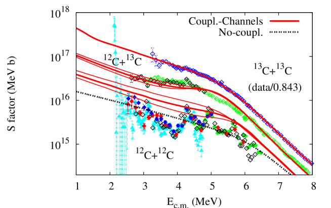
Figure 17: (Color online) $S$ factors for the fusion of ¹³C+¹³C trent , ¹²C+¹³C dayras ; tang1 and ¹²C+¹²C aguilera ; high ; maza ; becker ; spillane are compared to the coupled-channels calculations described in the text. The ¹³C+¹³C data have been divided by $S_{c}$ = 0.843 which optimizes the fit to the data. The thin solid curves show the error band due to the uncertainty in the octupole strength in ¹²C, $\beta_{3}$ = 0.90 $\pm$ 0.07. The black dashed curve is the no-coupling limit for ¹²C+¹²C.

The cross sections one obtains for the three fusion reactions discussed in this work, using the best fit parameters determined in the previous sections, and the shell model results described above, are compared to the data in Fig. 17 in terms of the $S$ factor. The data for ¹³C+¹³C have been divided by the scaling factor $S_{C}$ = 0.843 which results in an excellent agreement with the data. The calculations of the fusion of ¹²C+¹²C and ¹²C+¹³C are Ch12 and Ch26 calculations, respectively, which are similar to those discussed in section IV and V. The only difference is that the parameters for the mutual $(2^{+},3^{-})$ excitation in ¹²C have been replaced by shell model predictions brown .

The calculated $S$ factors for the fusion of ¹²C+¹²C and ¹²C+¹³C are essentially predictions because the parameters of ion-ion potential and the density of ¹³C were determined in the analysis of the ¹³C+¹³C fusion data, whereas the density of ¹²C was determined by a fit to the experimental point-proton distribution. The ¹²C+¹³C data dayras ; tang1 shown in Fig. 17 form a plateau between 2.5 and 4 MeV and has a peak near 4.3 MeV. These features are not quite reproduced by the calculation but the fit to the data is not poor; the fit to the data of Ref. dayras is stable with respect to the scaling factor $S_{c}$ and to an overall energy shift $\Delta E$ in the center of mass energy, i. e., the $\chi^{2}$ per data point has a minimum for $S_{c}$ = 1 and $\Delta E$ = 0.

Although there is still some uncertainty in the predicted $S$ factor for the fusion of ¹²C+¹²C, it appears that the calculation shown in Fig. 17 is consistent with the maxima of the measured peak cross sections. The peak at 4.924 MeV is within the error band of the calculation. The 3 low-energy (triangular shaped) data points are from Ref. spillane . They exceed the calculation tremendously but that is not a problem either because those 3 data points are questionable as discussed in Ref. sisyfus ; tang2 . The calculation (with its error band) is therefore expected to provide a useful guidance and an upper limit for the extrapolation to the low energies that are of interest to astrophysics.

VII Conclusions

We have explored the fusion of different combinations of carbon isotopes within the coupled-channels approach. The fusion cross section is determined by ingoing-wave-boundary conditions that are imposed at the minimum of the pocket in the entrance channel potential. It turned out that the measured cross sections for the fusion of ¹³C+¹³C cannot be explained accurately at low energies when a standard Woods-Saxon potential is applied in the calculations. However, the data can be explained fairly well by applying the shallow potential that is produced by the M3Y+repulsion potential. This is a characteristic feature of the fusion hindrance phenomenon which has been observed in many medium-heavy systems. One reason the shallow potential makes it possible to explain the carbon data by coupled-channels calculations is that the high-lying excitations become closed channels at low center-of-mass energies, not only with respect to reactions but also to fusion.

The coupled-channels calculations are surprisingly sensitive to mutual excitations and this seems to be justified by the comparison to the data. Thus the calculations that include one-phonon excitations alone cannot explain the data so well, neither when the standard Woods-Saxon nor the M3Y+repulsion potential is applied. The data are reproduced much better when mutual excitations are included and the shallow M3Y+repulsion potential is applied. The reason is that the direct coupling to these high-lying states is proportional to the second derivative of the ion-ion potential and this quantity is much larger for the M3Y+repulsion than for the standard Woods-Saxon potential because of the strong repulsion.

The large sensitivity to the excitation of high-lying states is particularly critical when the mutual excitations involve the strong octupole excitation of ¹²C. The uncertainty in the strength of the octupole excitation, and also in the strength of transitions to high-lying states that are built on the $2^{+}$ and $3^{-}$ states, makes it difficult to predict the fusion cross sections very accurately when ¹²C is involved. However, by adopting the nuclear structure properties of the high-lying states predicted by the shell model, one obtains a fairly good description of the ¹²C+¹³C fusion data.

The prediction of the cross section for the fusion of ¹²C+¹²C, based on the ingoing-wave-boundary conditions and the shell model prediction of the coupling to high-lying states, exceeds most of the measured cross sections and is consistent with the maxima of the observed peak cross sections. Thus it appears that the calculation provides an upper limit of the measured cross sections. The calculation is therefore expected to provide an upper limit for the extrapolation of cross sections into the unexplored territory of very low energies.

On the experimental side it is very important to get a better absolute normalization of the measured fusion cross sections. The current systematic errors are fairly large. This was exploited in the analysis of the ¹³C+¹³C fusion data by focusing on the shape of the measured cross section, whereas the absolute normalization was treated as an adjustable parameter. In this way it was possible to calibrate the M3Y+repulsion potential and achieve an excellent fit to the data. It is of great interest to know whether the renormalization that was applied to the data can be justified by more accurate measurements.

Acknowledgments. The authors are grateful to B. A. Brown for providing the shell model calculations. This work was supported by the U.S. Department of Energy, Office of Nuclear Physics, contract no. DE-AC02-06CH11357. One of us (X.T.) is supported by the NSF under Grant No. PHY-0758100 and PHY-0822648, and the National Natural Science Foundation of China under Grant No. 11021504, and the University of Notre Dame.

VIII Appendix: Couplings

The matrix elements of the couplings between two heavy ions are generated by matrix elements of the static or dynamic deformation amplitudes $\alpha_{\lambda\mu}$ (see for example Ref. alge ). The matrix elements are expressed in terms of the reduced matrix elements $\langle||\alpha_{\lambda}||\rangle$,

$$\langle I_{2}M_{2}|\alpha_{\lambda\mu}|I_{1}M_{1}\rangle=\langle I_{1}M_{1}\lambda\mu|I_{2}M_{2}\rangle\ \frac{\langle I_{2}||\alpha_{\lambda}||I_{1}\rangle}{\sqrt{2I_{2}+1}}.$$ (14)

The off-diagonal reduced matrix elements can be extracted from the measured $B(E\lambda)$ values according to the formula

$$B(E\lambda,I_{2}\rightarrow I_{1})=\bigl{(}\frac{3Ze^{2}R_{C}^{\lambda}}{4\pi}\bigr{)}^{2}\ \frac{|\langle I_{2}||\alpha_{\lambda}||I_{1}\rangle|^{2}}{2I_{2}+1}.$$ (15)

If the $B$-value is expressed in Weisskopf units the relation is

$$B(E\lambda)_{W.u.}=\frac{[Z(\lambda+3)]^{2}}{4\pi}\frac{|\langle I_{2}||\alpha_{\lambda}||I_{1}\rangle|^{2}}{2I_{2}+1}.$$ (16)

The diagonal matrix elements, on the other hand, can be obtained from the measured quadrupole moments,

$$Q_{II}=\sqrt{\frac{16\pi}{5}}\ \frac{3ZeR_{C}^{2}}{4\pi}\ \langle II|\alpha_{20}|II\rangle.$$ (17)

They are related to the intrinsic quadrupole moments $Q_{0}$ and the $K$ quantum number by

$$Q_{II}=\langle IK20|IK\rangle\ \langle II20|II\rangle\ Q_{0}.$$ (18)

For a deformed nucleus with a static deformation $\beta_{\lambda}$ the deformation amplitude is $\alpha_{\lambda\mu}$ = $\beta_{\lambda}D^{\lambda}_{\mu 0}({\hat{e}})$, where ${\hat{e}}$ is the orientation of the symmetry axis. In this case the expressions for the matrix elements between states $|IKM\rangle$ are

$$\langle I_{2}KM|\alpha_{\lambda 0}|I_{1}KM\rangle=\beta_{\lambda}\sqrt{\frac{2I_{1}+1}{2I_{2}+1}}\ \langle I_{1}M\ \lambda 0|I_{2}M\rangle\ \langle I_{1}K\ \lambda 0|I_{2}K\rangle.$$ (19)

This implies (by comparing to Eq. (14) that the reduced matrix elements are

$$\langle I_{2}||\alpha_{\lambda}||I_{1}\rangle=\beta_{2}\sqrt{2I_{1}+1}\ \langle I_{1}K\ \lambda 0|I_{2}K\rangle.$$ (20)

$$B(E\lambda)_{W.u.}=\frac{[Z(\lambda+3)]^{2}}{4\pi}\ \beta_{\lambda}^{2}\ \frac{2I_{1}+1}{2I_{2}+1}\ \langle I_{1}K\ \lambda 0|I_{2}K\rangle^{2}.$$ (21)

Table 1: Parameters of the densities that are used in calculating the M3Y+repulsion potential. The second column shows the radius $R$; the diffuseness was kept fixed at $a$ = 0.44 fm and the third column is the calculated rms radius. Also shown is the diffuseness $a_{r}$ that is used in calculating the repulsive part of the potential, the value of scaling factor $S_{c}$ that optimizes the fit to the ¹³C+¹³C fusion data trent , and the $\chi^{2}/N$. The last 3 lines show the radii that are consistent with the rms radii of the point-proton (pp) and matter distributions of ¹²C and ¹³C.

Nucleus	R (fm)	rms (fm)	$a_{r}$ (fm)	$S_{c}$	$\chi^{2}/N$
13C	2.17	2.345	0.33	1	2.75
13C	2.28	2.407	0.31	0.843	1.00
12C (pp)	2.155	2.337(2)
13C (pp)	2.146	2.332(3)
13C, Eq. (3)	2.228	2.378

Table 2: Properties of E2 and E3 transitions in ¹²C and ¹³C ENDSF . The intrinsic quadrupole moments have been extracted from the lowest quadrupole transitions.

Nucleus	State	Ex (MeV)	Transition	B(E$\lambda$) (W.u.)	$\beta_{\lambda}^{C}$
12C	$0^{+}_{1}$	0		$Q_{0}$ =-19.5 fm2	0.570
	$2^{+}$	4.439	E2: $0_{1}^{+}\rightarrow 2^{+}$	4.65(26)	0.570
	$0_{2}^{+}$	7.654	E2: $2^{+}\rightarrow 0_{2}^{+}$	8.0(11)	0.236
	$3^{-}$	9.641	E3: $0_{1}^{+}\rightarrow 3^{-}$	12(2) ENDSF	0.90(7)
13C	$1/2^{-}$	0		$Q_{0}$ = -17.9 fm2	0.495
	$3/2^{-}$	3.6845	E2: $1/2^{-}\rightarrow 3/2^{-}$	3.5(8)	0.495
	$5/2^{-}$	7.547	E2: $1/2^{-}\rightarrow 5/2^{-}$	3.1(2)	0.465
	$5/2^{+}$	3.8538	E3: $1/2^{-}\rightarrow 5/2^{+}$	10(4)	0.82

References

- (1) L. R. Gasques et al., Phys. Rev. C 72, 025806 (2005).
- (2) S. Trentalange, S. C. Wu, J. L. Osborne, and C. A. Barnes, Nucl. Phys. A483, 406 (1988).
- (3) J. L. Charvet, R. Dayras, J. M. Fieni, S. Joly, and J. L. Uzureau, Nucl. Phys. A376, 292 (1982).
- (4) R. A. Dayras, R. G. Stokstad, Z. E. Switkowski, and R. M. Wieland, Nucl. Phys. A265, 153 (1976).
- (5) M. Notani et al., Nucl. Phys. A824, 192c (2010).
- (6) R. A. Broglia and A. Winther, Frontiers in Physics Lecture Notes Series: Heavy-ion Reactions, Vol 84. (Addison-Wesley, Redwood City, CA, 1991).
- (7) S. Misicu and H. Esbensen. Phys. Rev. C 75, 034606 (2007).
- (8) H. Esbensen, Phys. Rev. C 77, 054608 (2008).
- (9) C. L. Jiang, B. B. Back, H. Esbensen, R. V. F. Janssens, and K.E. Rehm, Phys. Rev. C 73, 014613 (2006).
- (10) C. L. Jiang et al., Phys. Rev. Lett. 89, 052701 (2002).
- (11) C. L. Jiang, K. E. Rehm, B. B. Back, and R. V. F. Janssens, Phys. Rev. C 75, 015803 (2007); Phys. Rev. C 79, 044601 (2009).
- (12) D. A. Bromley, J. A. Kuehner, and E. Almquist, Phys. Rev. Lett. 4, 365 (1960).
- (13) E. Almquist, D. A. Bromley, and J. A. Kuehner, Phys. Rev. Lett. 4, 515 (1960).
- (14) G. Michaud, Phys. Rev. C 8, 525 (1973).
- (15) B. Dasmahapatra, B. Cujec, and F. Lahlou Nucl. Phys. A384, 257 (1982).
- (16) H. Esbensen, Phys. Rev. C 68, 034604 (2003).
- (17) H. Esbensen and S. Misicu, Phys. Rev. C 76, 054609 (2007).
- (18) G. Bertsch, J. Borosowicz, H. McManus, and W. G. Love, Nucl. Phys. A284, 399 (1977).
- (19) H. De Vries, C.W. De Jager and C. De Vries, Atomic Data Nuclear Data Tables, 36, 495-536 (1987).
- (20) I. Angeli, Atomic Data and Nuclear Data Tables, 87, 185-206 (2004).
- (21) H. Esbensen, C. L. Jiang, and A. M. Stefanini, Phys. Rev. C 82. 054621 (2010).
- (22) Evaluated Nuclear Data Structure Files, Nuclear Data Center, Brookhaven Nat. Lab. [http://www.ndc.bnl.gov].
- (23) W. J. Vermeer, M. T. Esat, J. A. Kuehner, R. H. Spear, A. M. Baxter, and S. Hinds, Phys. Lett. 122B, 23 (1983).
- (24) J. Lee, M. B. Tsang and W. G. Lynch, Phys. Rev. C 75, 064320 (2007).
- (25) J. M. Quesada, G. Pollarolo, R. A. Broglia, and A. Winther, Nucl. Phys. A442, 381 (1985).
- (26) H. Esbensen and S. Landowne, Nucl. Phys. A492, 473 (1989).
- (27) M. H. MacFarlane and S. C. Pieper, Code Ptolemy: Argonne Laboratory Report No. ANL-76-11 (1978).
- (28) M. G. Mazarakis and W. E. Stephens, Phys. Rev. C 7,1280 (1973).
- (29) M. D. High and B. Cujec, Nucl. Phys. 282, 181 (1977).
- (30) E. F. Aguilera et al., Phys. Rev. C 73, 064601 (2006).
- (31) H. W. Becker, K. U. Kettner, C. Rolfs, H. P. Trautvetter, Z. Phys. 303, 305 (1981).
- (32) T. Spillane et al., Phys. Rev. Lett. 98, 122501 (2007).
- (33) D. G. Yakovlev, M. Beard, L. R. Gasques, and M. Wiescher, Phys. Rev. C 82, 044609 (2010).
- (34) M. Alcorta et al., Phys. Rev. Lett. 106, 172701 (2011).
- (35) B. A. Brown (private communications.)
- (36) J. Zickefoose, U. Conn. thesis (2010).
- (37) M. Notani, X. Tang et al., University of Notre Dame (unpublished information, 2011).