ENERGY-MOMENTUM TENSORS WITH WORLDLINE NUMERICS

Abstract

We apply the worldline formalism and its numerical Monte-Carlo approach to computations of fluctuation induced energy-momentum tensors. For the case of a fluctuating Dirichlet scalar, we derive explicit worldline expressions for the components of the canonical energy-momentum tensor that are straightforwardly accessible to partly analytical and generally numerical evaluation. We present several simple proof-of-principle examples, demonstrating that efficient numerical evaluation is possible at low cost. Our methods can be applied to an investigation of positive-energy conditions.

1 Introduction

It has been over five decades since Casimir predicted a negative interaction energy density and a corresponding attractive force[1] between two perfectly conducting plates in a vacuum which impose boundary conditions on the quantized electromagnetic field. Although the theory of the Casimir effect has become a well developed field in recent years[2], it still serves as a paradigmatic test case for exploring the diversity of phenomena within quantum field theories. In the first place, interaction energies, pressures and forces caused by boundary conditions (BCs) imposed on a quantum field are of particular relevance, as they constitute phenomenological observables of the Casimir effect and can be directly related to experiment. From a more theoretical perspective, this information is more generally encoded in the expectation value of the energy-momentum tensor (EMT) of the fluctuating field.

Beyond the direct phenomenological application, the energy-momentum tensor is also at the center of interest since it serves as a source term for the gravitational field if the quantum field is coupled to gravity. For instance, the energy-momentum tensor is needed in order to study how the Casimir energy falls in a gravitational field[3]. For usual Casimir force calculations, the fact that Casimir energies can generically be negative is not a problem at all, as it is similar to negative binding energies in bound state systems. However, in connection with general relativity, negative energy densities can be puzzling. Such energy densities may be in conflict with restrictions imposed on the energy-momentum tensor in order to avoid exotic phenomena such as superluminal travel, wormholes or time machines. Indeed, the Casimir effect violates particular restrictions such as the weak energy condition (WEC), $\langle\hat{T}_{\mu\nu}V^{\mu}V^{\nu}\rangle\geq 0$ with $V^{\mu}$ being a timelike vector, or the null energy condition (NEC), $\langle\hat{T}_{\mu\nu}V^{\mu}V^{\nu}\rangle\geq 0$ with $V^{\mu}$ being a null vector[4, 5]. By contrast, both conditions are obeyed by classical physics.

A somewhat weaker condition that is still sufficient to rule out exotic phenomena is the averaged null energy condition (ANEC) which requires that the null energy condition has to hold only when integrated along a complete geodesic. The ANEC has been found to be satisfied in all Casimir examples studied so far on flat Minkowski space (even though it can be violated on compact flat or curved spaces[6]). An investigation of the ANEC in specific Casimir configurations is typically involved, as certain components of the energy-momentum tensor need to be known along a complete geodesic. However, the physically interesting geodesics which appear to collect negative energy densities along the geodesic are typically directed towards a surface and thus hit the surface at some point. In such a case, the average acquires a generically large positive contribution from the surface itself which – though nonuniversal – is likely to exceed the negative Casimir contributions by far. Relevant configurations that avoid the discussion of large nonuniversal contributions therefore need to have holes through which a geodesic can pass. In fact, the case of a single plate with a hole has been found to obey the ANEC[7].

As is obvious from these considerations, a general study of energy conditions in Casimir configurations requires a theoretical framework that is capable of dealing with the energy-momentum tensor in arbitrary geometries. Standard computations of Casimir energy momentum tensors[8, 9, 10, 11, 12] are usually based on mode summation/expansion, image charge methods or similar techniques which are suited for specific simple geometries. In the present work, we report on progress using the worldline approach[13] to the Casimir effect for the case of a Dirichlet scalar field[14, 15] which has meanwhile been used to study a variety of nontrivial Casimir configurations[16, 17, 18, 19]. We show that the worldline approach can straightforwardly be generalized to study Casimir energy-momentum tensors. We discuss the similarities and differences with conventional interaction energy computations and verify the resulting algorithm with the help of known simple examples.

2 Worldline Formalism for composite operators

We investigate the energy-momentum tensor of a minimally coupled quantum scalar field $\hat{\Phi}$ with zero mass which shall be defined on a $d+1$-dimensional domain $\mathcal{D}$. On the boundary $\partial\mathcal{D}$ that we consider as static we impose Dirichlet boundary conditions. The canonical energy-momentum tensor operator of $\hat{\Phi}$ reads

$$\hat{T}_{\mu\nu}(x,t):=\lim_{{x}\to{x}^{\prime}}\left[\partial_{\mu}\hat{\Phi}\partial^{\prime}_{\nu}\hat{\Phi}^{\prime}-\frac{1}{2}g_{\mu\nu}\left(\partial_{\alpha}\hat{\Phi}\partial^{\prime\alpha}\hat{\Phi}^{\prime}-\sigma(x)\hat{\Phi}\hat{\Phi}^{\prime}\right)\right],$$ (1)

where we have employed a point-splitting procedure in the spatial coordinates for regularization. The background potential $\sigma(x)$ can in principle be arbitrary but will later specifically be used to impose Dirichlet BCs. For our study of the energy conditions, we need to compute the vacuum expectation value $\left\langle\hat{T}_{\mu\nu}\right\rangle$ of the EMT. For instance, for the null energy condition, we have to evaluate the combination

$$\left\langle\hat{T}_{\mu\nu}V^{\mu}V^{\nu}\right\rangle=\left\langle\hat{T}_{00}+\hat{T}_{zz}\right\rangle=T_{00}+T_{zz},$$ (2)

where we have choosen the null vector $V^{\mu}$ in $z$ direction: $V^{\mu}=(1,0,\ldots,0,1)$. In a next step we expand the scalar field $\hat{\Phi}$ in terms of momentum modes $\psi_{n}$. These momentum modes are defined as eigenmodes of the Laplacian in the presence of $\sigma(x)$,

$$\left(-{\nabla}^{2}+\sigma(x)\right)\psi_{n}(x)=k_{n}^{2}\psi_{n}(x),$$ (3)

with $k_{n}^{2}$ denoting the eigenvalue. We now introduce the propagator $G({x},{x}^{\prime},k)$ of the corresponding Helmholtz equation

$${\left(-{\nabla}^{2}+\sigma(x)-k^{2}\right)G({x},{x}^{\prime},k)=\delta({x}-{x}^{\prime})}$$ (4)

which has the spectral representation

$$G({x},{x}^{\prime},k)=\sum_{n}\frac{\psi_{n}(x)\psi_{n}^{*}(x^{\prime})}{k_{n}^{2}-k^{2}-i\varepsilon}.$$ (5)

The components of the energy-momentum tensor in Eq. (2) can now be expressed solely in terms of $G({x},{x}^{\prime},k)$. As we are interested in the effect of the background potential $\sigma(x)$ in comparison to the vacuum case $\sigma=0$, we normalize the EMT with respect to the trivial vacuum by subtracting the free Green’s function $G_{0}({x},{x}^{\prime},k)$ obtained from Eq. (4) for $\sigma=0$. This corresponds to removing the $\sigma$-independent divergence,

$$\langle\hat{T}_{00}({x},t)\rangle={} \lim_{{x}\to{x}^{\prime}}\int_{0}^{\infty}\frac{\mathrm{d}k}{\pi}\left(k^{2}+\frac{1}{2}{\nabla}\cdot\left({\nabla}+{\nabla}^{\prime}\right)\right)\operatorname{Im}\left[(G-G_{0})({x},{x}^{\prime},k)\right],$$ (6)

$$\langle\hat{T}_{zz}({x},t)\rangle={} \lim_{{x}\to{x}^{\prime}}\int_{0}^{\infty}\frac{\mathrm{d}k}{\pi}\left(\partial_{z}\partial_{z^{\prime}}-\frac{1}{2}{\nabla}\cdot\left({\nabla}+{\nabla}^{\prime}\right)\right)\operatorname{Im}\left[(G-G_{0})({x},{x}^{\prime},k)\right].$$ (7)

The whole formalism works, of course, for any field configuration $\sigma(x)$. In the following, we focus on $\sigma$ backgrounds that induce Dirichlet BCs on $\partial\mathcal{D}$. For this, we schematically use

$$\sigma(x)=\lambda\,\delta\left({x-x_{\partial\mathcal{D}}}\right),\quad{x_{\partial\mathcal{D}}\in\partial\mathcal{D},}$$ (8)

and take the Dirichlet limit $\lambda\to\infty$ [20]. The EMT in Eq. (6) and (7) is then finite on $\mathcal{D}$ where the potential $\sigma$ vanishes. There remain, however, divergences on the boundary $\partial\mathcal{D}$ due to the Dirichlet limit. These can be interpreted as the infinite amount of energy needed to constrain a scalar quantum field on all momentum scales to satisfy the Dirichlet constraint on the boundary[20].

Interpreting the eigenvalue problem (3) as a ficticious quantum mechanical Schrödinger problem with Hamiltonian $H=-\nabla^{2}+\sigma(x)$, the Green’s function corresponds to a quantum mechanical propagator Fourier transformed to energy space, which can be written as a Feynman path integral in position space. The vacuum-subtracted path integral representation of the propagator then results in

$$(G-G_{0})({x},{x}^{\prime},k)={} i\int\limits_{0}^{\infty}\mathrm{d}s\,e^{isk^{2}}\int\limits_{x^{\prime}{=x(0)}}^{x{=x(T)}}\mathcal{D}{x}(\tau)e^{i\int\limits_{0}^{s}\mathrm{d}\tau\frac{\dot{{x}}^{2}}{4}}\left(e^{-i\int\limits_{0}^{s}\mathrm{d}\tau\,\sigma({x})}-1\right)$$

$$={} \int\limits_{0}^{\infty}\mathrm{d}T\,e^{-Tk_{E}^{2}}\int\limits_{x^{\prime}}^{x}\mathcal{D}{x}(\tau)e^{-\int\limits_{0}^{T}\mathrm{d}\tau\frac{\dot{{x}}^{2}}{4}}\left(e^{-\int\limits_{0}^{T}\mathrm{d}\tau\,\sigma({x})}-1\right),$$ (9)

where $s$ is a ficticious quantum mechanical time, so-called propertime. We have formally made Wick rotations both in the $s$ and $k$ planes so that $s=-iT$ and $k_{E}=ik$ to cast the expression above in Euclidean form.

In contrast to previous calculations of effective interaction energies for the Casimir effect and similar setups which required path integrals only over closed loops, here we need to compute path integrals of open worldlines from ${x}^{\prime}$ to ${x}$. This can conveniently be done with the $d$ loop algorithm[21]. The path integral is normalized here implicitly such that the free path integral yields the standard free propagator,

$$\int\limits_{x^{\prime}}^{x}\mathcal{D}x(\tau)e^{-\int\limits_{0}^{T}\mathrm{d}\tau\frac{\dot{x}^{2}}{4}}=\frac{e^{-\frac{({x}-{x}^{\prime})^{2}}{4T}}}{\left(4\pi T\right)^{\frac{d}{2}}}.$$ (10)

This normalization is made explicit by the following shorthand notation

$$\frac{e^{-\frac{({x}-{x}^{\prime})^{2}}{4T}}}{\left(4\pi T\right)^{\frac{d}{2}}}\left\langle\mathcal{O}\right\rangle_{xx^{\prime}}:=\int\limits_{x^{\prime}}^{x}\mathcal{D}x(\tau)e^{-\int\limits_{0}^{T}\mathrm{d}\tau\frac{\dot{x}^{2}}{4}}\mathcal{O}.$$ (11)

Then Eq. (2) can be written as

$$(G-G_{0})({x},{x}^{\prime},k=-ik_{E})={} \int\limits_{0}^{\infty}\mathrm{d}T\,e^{-Tk_{E}^{2}}\frac{e^{-\frac{({x}-{x}^{\prime})^{2}}{4T}}}{\left(4\pi T\right)^{\frac{d}{2}}}\left\langle e^{-\int\limits_{0}^{T}\mathrm{d}\tau\,\sigma(x)}-1\right\rangle_{{xx^{\prime}}}.$$ (12)

In the Dirichlet limit the last term can be simplified

$$\left\langle e^{-\int\limits_{0}^{T}\mathrm{d}\tau\,\sigma(x)}-1\right\rangle_{{xx^{\prime}}}\!\!\!\!\!=\left\{\begin{array}[]{cl}-1&\mbox{if $x(\tau)$ intersects a boundary}\\ 0&\mbox{{otherwise}}\end{array}\right\}=-\left\langle\Theta\left(T-T_{\text{min}}\right)\right\rangle_{{xx^{\prime}}}$$ (13)

which means that only loops $x(\tau)$ that violate the boundary conditions lead to deviations from the trivial vacuum and thus contribute to the path integral. The quantity $T_{\text{min}}$ denotes the minimum propertime needed for a given worldline to propagate from $x^{\prime}$ to $x$ and simultaneously intersect a boundary in between. If $T$ is too small the particle has to propagate on a straight line from $x^{\prime}$ to $x$. If $T$ is sufficiently long the diffusive Brownian motion process behind the path integral creates random detours that can eventually intersect the boundaries. We may choose our integration contour in the $k_{E}$ plane in such a manner that the imaginary part of the integral is already taken into account by carrying out the $k_{E}$ integrations in (6) and (7) along the real axis, indeed this is the effect of the Wick rotation. These considerations lead us to a compact representation of the EMT components required, e.g., for the null energy condition:

$$\langle\hat{T}_{00}({x},t)\rangle(I)={} \frac{1}{(4\pi)^{\frac{d+1}{2}}}\int\limits_{0}^{\infty}\frac{\mathrm{d}T}{2T^{\frac{d+3}{2}}}e^{-\frac{({x}-{x}^{\prime})^{2}}{4T}}\left\langle\Theta\left(T-T_{\text{min}}\right)\right\rangle_{{xx^{\prime}}},$$ (14)

$$\langle\hat{T}_{zz}({x},t)\rangle(I)={} -\frac{1}{(4\pi)^{\frac{d+1}{2}}}\partial_{z}\partial_{z^{\prime}}\int\limits_{0}^{\infty}\frac{\mathrm{d}T}{T^{\frac{d+1}{2}}}e^{-\frac{({x}-{x}^{\prime})^{2}}{4T}}\left\langle\Theta\left(T-T_{\text{min}}\right)\right\rangle_{{xx^{\prime}}},$$ (15)

$$\langle\hat{T}_{00}({x},t)\rangle(II)={} -\frac{1}{(4\pi)^{\frac{d+1}{2}}}{\nabla}\cdot\left({\nabla}+{\nabla}^{\prime}\right)\int\limits_{0}^{\infty}\frac{\mathrm{d}T}{2T^{\frac{d+1}{2}}}e^{-\frac{({x}-{x}^{\prime})^{2}}{4T}}\left\langle\Theta\left(T-T_{\text{min}}\right)\right\rangle_{{xx^{\prime}}}$$

$$={} -\langle\hat{T}_{zz}({x},t)\rangle(II),$$ (16)

where the limit ${x}\to{x}^{\prime}$ is implicitly understood from now on. From the last identity, it is, for instance, obvious that the NEC only involves $\left\langle\hat{T}_{\mu\nu}V^{\mu}V^{\nu}\right\rangle=T_{00}(I)+T_{zz}(I)$. We emphasize that the angle brackets are used in two different contexts: on the l.h.s. $\left\langle\dots\right\rangle$ denotes the vacuum expectation of a composite quantum operator, whereas on the r.h.s. $\left\langle\dots\right\rangle_{{xx^{\prime}}}$ denotes the expectation value of the path integral, that is the average over an ensemble of open worldlines.

3 Energy momentum tensor for a single plate

With these general considerations, we can now compute the EMT components in the case where the boundary is one single plate at $z=0$ with the $z$ axis being its normal.

3.1 Analytical calculation for the single plate

Analytical results for the single plate are easily obtained through explicit calculation of the Green’s function using the method of images. After regularization one finds

$$(G-G_{0})({x},{x}^{\prime};k)=-\varphi({\xi},{x}^{\prime})$$ (17)

in which $\varphi({\xi},{x}^{\prime})$ denotes the field at ${x}^{\prime}:=({x}^{\prime}_{\parallel},z^{\prime})$ produced by a point source sitting at ${\xi}:=({x}_{\parallel},-z)$. Also ${x}:=({x}_{\parallel},z)$, with $z$ and $z^{\prime}$ being the distances from the plate. The explicit forms of the field $\varphi$ in two and three dimensions are given by $\varphi_{d=2}=\frac{1}{2\pi}K_{0}(-ik|{x}-{x}^{\prime}|)$ and $\varphi_{d=3}=\frac{e^{ik|{x}-{x}^{\prime}|}}{4\pi|{x}-{x}^{\prime}|}$, respectively. Using them it is straightforward to show that

$$\left\langle\hat{T}_{00}\right\rangle_{\mathrm{d=2}}\mathrm{(I)}\ =\quad\!\frac{1}{32\pi}\frac{1}{z^{3}}, \left\langle\hat{T}_{00}\right\rangle_{\mathrm{d=3}}\mathrm{(I)}\ =\quad\!\frac{1}{32\pi^{2}}\frac{1}{z^{4}},$$ (18)

$$\left\langle\hat{T}_{00}\right\rangle_{\mathrm{d=2}}\mathrm{(II)} =-\frac{1}{16\pi}\frac{1}{z^{3}}, \left\langle\hat{T}_{00}\right\rangle_{\mathrm{d=3}}\mathrm{(II)} =-\frac{3}{32\pi^{2}}\frac{1}{z^{4}},$$ (19)

$$\left\langle\hat{T}_{zz}\right\rangle_{\mathrm{d=2}}\mathrm{(I)}\ =-\frac{1}{16\pi}\frac{1}{z^{3}}, \left\langle\hat{T}_{zz}\right\rangle_{\mathrm{d=3}}\mathrm{(I)}\ =-\frac{3}{32\pi^{2}}\frac{1}{z^{4}}.$$ (20)

3.2 Worldline calculation for the single plate

For the computation of the expectation value in Eq. (14) and (16), we need to evaluate the worldline $\Theta$ function, i.e., we need to find the condition under which a loop in our ensemble intersects the plate (see Fig. 1 for a sketch).

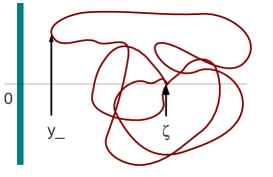
Figure 1: Sketch of the single plate setup.

After rescaling the loops for numerical convenience[14]

$$x(Tt)\to\sqrt{T}y(t),\,\,t\in[0,1]\quad\Rightarrow\quad\int_{x^{\prime}}^{x}\mathcal{D}x(\tau)e^{-\int\limits_{0}^{T}\mathrm{d}\tau\frac{\dot{x}^{2}}{4}}\to\int_{x^{\prime}/\sqrt{T}}^{x/\sqrt{T}}\mathcal{D}y(t)e^{-\int\limits_{0}^{1}\mathrm{d}t\frac{\dot{y}^{2}}{4}},$$ (21)

we find in the limit $x^{\prime}\to x$, that is, $z^{\prime}\to z$, the intersection condition

$$\sqrt{T}y_{-}+z\leq 0\ \Longrightarrow\ \Theta\left(T-T_{\text{min}}\right)=\Theta\left(T-\frac{z^{2}}{y_{-}^{2}}\right),$$ (22)

where $z$ denotes the distance from the plate and $y_{-}$ denotes the point of a loop that is closest to the plate, see Fig. 1. The quantity $y_{-}$ is the only information we need about each loop. Since the worldline distributions factorize with respect to their position space components, we only need 1-dimensional loops. In $d=2$ the $T_{00}$ component of the EMT then reads

$$\left\langle\hat{T}_{00}\right\rangle=\left\langle\hat{T}_{00}\right\rangle(\text{I})+\left\langle\hat{T}_{00}\right\rangle(\text{II})={} \frac{1}{(4\pi)^{\frac{3}{2}}}\frac{1}{z^{3}}\left(\frac{\langle\left|y_{-}\right|^{3}\rangle}{3}-\langle\left|y_{-}\right|\rangle\right)$$ (23)

$$={} \frac{1}{(4\pi)^{\frac{3}{2}}}\frac{1}{z^{3}}\left(\frac{\sqrt{\pi}}{4}-\frac{\sqrt{\pi}}{2}\right)$$ (24)

with the corresponding analytical values in the second line. In Table 3.2 we compare our analytical and numerical results for two different ensembles with $N$ loops per ensemble and $ppl$ points per loop.

Worldline results for the single plate in $d=2$. $ppl$, $N$ $\langle\left|y_{-}\right|\rangle$ $\frac{\sqrt{\pi}}{2}$ $\langle\left|y_{-}\right|^{3}\rangle$ $\frac{3\sqrt{\pi}}{4}$ $2^{14},\,10^{4}$ $0.8789\pm 0.0046$ 0.8862 $1.3018\pm 0.0210$ 1.3293 $2^{18},\,5\cdot 10^{5}$ $0.8841\pm 0.0007$ 0.8862 $1.3236\pm 0.0029$ 1.3293

The error corresponds to the statistical uncertainty only and it decreases like $1/\sqrt{N}$ as expected. The systematic error that is not displayed explicitly is governed by the discretization of the loops (i.e. by $ppl$). A larger number of points per loop improves our results. As is known from previous calculations of the Casimir energy using worldline numerics the numerical values approach the analytical values from below, that is the discretized loops are smaller than the continuous ones.

The same analysis can be done for three spatial dimensions where we find

$$\left\langle\hat{T}_{00}\right\rangle={} \frac{1}{(4\pi)^{2}}\frac{1}{z^{4}}\left(\frac{\langle\left|y_{-}\right|^{4}\rangle}{4}-\frac{3\langle\left|y_{-}\right|^{2}\rangle}{2}\right)$$ (25)

$$={} \frac{1}{(4\pi)^{2}}\frac{1}{z^{4}}\left(\frac{1}{2}-\frac{3}{2}\right).$$ (26)

The structure of the result is, of course, identical but the exponents of our loop variable and coefficients have changed. In Table 3.2 we show our worldline results. Just as in the two-dimensional case we again see the decrease of errors with increasing number of loops and $ppl$. In both cases, these results confirm the violation of the weak energy condition by the single-plate configuration in agreement with Ref. gr-qc/0205134.

Worldline results for the single plate in $d=3$. $ppl$, $N$ $\langle\left|y_{-}\right|^{2}\rangle$ $1$ $\langle\left|y_{-}\right|^{4}\rangle$ $2$ $2^{14},\,10^{4}$ $0.9841\pm 0.0100$ $1.0000$ $1.9610\pm 0.0488$ $2.0000$ $2^{18},\,5\cdot 10^{5}$ $0.9964\pm 0.0014$ $1.0000$ $1.9901\pm 0.0063$ $2.0000$

As a further check of our algorithm we compute the null energy condition along the $z$ axis

$$\left\langle\hat{T}_{00}+\hat{T}_{zz}\right\rangle={} \frac{1}{(4\pi)^{\frac{d+1}{2}}}\frac{1}{z^{d+1}}\left(\frac{\langle\left|y_{-}\right|^{d+1}\rangle}{d+1}-\frac{d}{2}\langle\left|y_{-}\right|^{d-1}\rangle\right)$$ (27)

which is also violated[4]. Comparing with the analytical results again shows that our algorithm reproduces the expected values within the numerical precision set by the parameters of our loop ensemble, viz. the number of points per loop $ppl$ and the number of loops $N$.

4 Energy density for two parallel plates

Let us now turn to the classic Casimir configuration of two infinite parallel plates separated by a distance $a$ imposing Dirichlet BCs on the fluctuating scalar field. However, because our energy-momentum tensor is finite everywhere except for $\partial\mathcal{D}$ we are not only able to compute energy conditions or EMT components but actually also parts of components. In the following, we focus on $T_{00}(I)$, cf. Eq. (14).

4.1 Analytical calculation for parallel plates

As before $T_{00}(I)$ may be calculated by means of the traditional Green’s function approach and the method of images which gives

$$(G-G_{0})({x},{x}^{\prime};k)=\sum_{q\in\mathbb{Z}/\{0\}}\varphi({x}_{q},{x}^{\prime})-\sum_{q\in\mathbb{Z}}\varphi({\xi}_{q},{x}^{\prime}).$$ (28)

Here the vectors ${x}_{q}:=({x}_{\parallel},z+2qa),~{}{\xi}_{q}:=({x}_{\parallel},-z+(2q+1)a)$ were introduced. This time, $z$ measures the distance from the plates in a coordinate system centered in the middle of the plates. Introducing the dimensionless coordinate $\zeta=z/a$ and inserting the expressions for $\varphi$ given above Eq. (18) yields for the region between the plates where $|\zeta|\leq 1/2$

$$\left\langle\hat{T}_{00}\right\rangle_{\mathrm{d=2}}\mathrm{(I)}={} -\frac{1}{32\pi}\frac{1}{a^{3}}\left(2\zeta_{R}\left(3\right)-\zeta_{H}\left(3,\frac{1}{2}+\zeta\right)-\zeta_{H}\left(3,\frac{1}{2}-\zeta\right)\right),$$

$$\left\langle\hat{T}_{00}\right\rangle_{\mathrm{d=3}}\mathrm{(I)}={} -\frac{1}{32\pi^{2}}\frac{1}{a^{4}}\left(2\zeta_{R}\left(4\right)-\zeta_{H}\left(4,\frac{1}{2}+\zeta\right)-\zeta_{H}\left(4,\frac{1}{2}-\zeta\right)\right),$$ (29)

with $\zeta_{R,H}$ denoting the Riemann and Hurwitz zeta functions, respectively.

4.2 Worldline calculation for parallel plates

The numerical worldline computation of

$$\left\langle\hat{T}_{00}\right\rangle\mathrm{(I)}={} \frac{1}{(4\pi)^{\frac{d+1}{2}}}\int\limits_{0}^{\infty}\frac{\mathrm{d}T}{2T^{\frac{d+3}{2}}}\left\langle\Theta\left(T-T_{\text{min}}\right)\right\rangle$$ (30)

for the Casimir plates is similar to the single-plate case. However, as there are now two plates we need two intersection conditions as well. Accordingly we must compute two points of each loop, viz. the points $y_{\pm}$ which are closest to the plates, see Fig. 2.

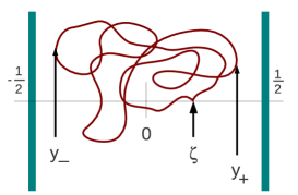
Figure 2: Sketch of Casimir’s parallel-plates configuration in units of $a=1$.

The corresponding value of $T_{\text{min}}$ is then easily found to be

$$\sqrt{T}y_{\pm}+{a}\left(\zeta\mp\frac{1}{2}\right)\leq 0\ \Longrightarrow\ \Theta\left(T-T_{\text{min}}\right)=\Theta\left(T-{a^{2}}\min\left[\left(\frac{\zeta\pm\frac{1}{2}}{y_{\mp}}\right)^{2}\right]\right).$$ (31)

The analytical findings of Eq. (29) compare favorably with the numerical data displayed in Fig. 3.

Figure 3: EMT component $T_{00}(I)$ in between two Casimir plates at a distance $a$ in two and three spatial dimensions, $\zeta=z/a$. The analytical result Eq. (29) (solid lines) is very well approximated by the numerical data.

4.3 Conclusion

We have studied Casimir energy-momentum tensors induced by a fluctuating minimally coupled scalar field obeying Dirichlet boundary conditions. We have demonstrated that this general problem can be formulated with the aid of the worldline approach to the Casimir effect. Contrary to simple interaction energy computations, the worldline approach for such composite operators now has to deal with open worldlines arising from the point-splitting procedure. As a proof of principle, we have been able to show that the numerical worldline approach to composite operators is able to reproduce analytically known results for the single- and parallel-plate cases at low cost and high efficiency. In particular, the single-plate case already shows violations of the weak as well as the null energy condition. Of course, the main goal of this project is to study more general classes of Casimir configurations which particularly allow for non-trivial tests of the averaged null energy condition. Work in this direction is in progress.

Acknowledgments: We have benefited from activities within the ESF Research Network CASIMIR. This work has been supported by the DFG under grant Gi328/5-1 (H.G.), Gi328/3-2 (I.H. and H.G.), GRK 1523 (M.S.) and partly by Conacyt (I.H.).

References

- [1] H.B.G. Casimir, Kon. Ned. Akad. Wetensch. Proc. 51, 793 (1948).
- [2] M. Bordag, U. Mohideen and V. M. Mostepanenko, Phys. Rept. 353, 1 (2001); K. A. Milton, “The Casimir effect: Physical manifestations of zero-point energy,” River Edge, USA: World Scientific (2001); J. Phys. Conf. Ser. 161, 012001 (2009) [arXiv:0809.2564 [hep-th]]; S. Y. Buhmann and D. G. Welsch, Prog. Quant. Electron. 31, 51 (2007) [arXiv:quant-ph/0608118]; T. Emig and R. L. Jaffe, J. Phys. AA 41, 164001 (2008) [arXiv:0710.5104 [quant-ph]]. M. Bordag, G. L. Klimchitskaya, U. Mohideen and V. M. Mostepanenko, Int. Ser. Monogr. Phys. 145, 1 (2009).
- [3] S. A. Fulling, K. A. Milton, P. Parashar, A. Romeo, K. V. Shajesh and J. Wagner, Phys. Rev. D 76, 025004 (2007) [hep-th/0702091 [HEP-TH]]; K. A. Milton, P. Parashar, K. V. Shajesh and J. Wagner, J. Phys. AA 40, 10935 (2007) [arXiv:0705.2611 [hep-th]]; K. V. Shajesh, K. A. Milton, P. Parashar and J. A. Wagner, J. Phys. AA 41, 164058 (2008) [arXiv:0711.1206 [hep-th]].
- [4] K. D. Olum and N. Graham, Phys. Lett. B 554, 175 (2003) [gr-qc/0205134]; N. Graham and K. D. Olum, Phys. Rev. D 67, 085014 (2003) [Erratum-ibid. D 69, 109901 (2004)] [hep-th/0211244].
- [5] D. Schwartz-Perlov and K. D. Olum, Phys. Rev. D 68 (2003) 065016 [Erratum-ibid. D 72 (2005) 069901] [hep-th/0307067].
- [6] M. Visser, Phys. Rev. D 54, 5116 (1996) [gr-qc/9604008].
- [7] N. Graham and K. D. Olum, Phys. Rev. D 72, 025013 (2005) [hep-th/0506136].
- [8] L. S. Brown and G. J. Maclay, Phys. Rev. 184, 1272 (1969).
- [9] K. A. Milton, Phys. Rev. D 68 (2003) 065020 [hep-th/0210081].
- [10] A. Scardicchio and R. L. Jaffe, Nucl. Phys. B 743, 249 (2006) [quant-ph/0507042].
- [11] K. Tywoniuk and F. Ravndal, quant-ph/0408163.
- [12] I. Brevik, S. A. Ellingsen and K. A. Milton, Int. J. Mod. Phys. A 25, 2270 (2010) [arXiv:0911.2688 [hep-th]].
- [13] C. Schubert, Phys. Rept. 355, 73 (2001) [arXiv:hep-th/0101036].
- [14] H. Gies, K. Langfeld and L. Moyaerts, JHEP 0306, 018 (2003); arXiv:hep-th/0311168.
- [15] H. Gies and K. Klingmuller, Phys. Rev. D 74 (2006) 045002 [quant-ph/0605141].
- [16] H. Gies and K. Klingmuller, Phys. Rev. Lett. 97, 220405 (2006) [arXiv:quant-ph/0606235].
- [17] A. Weber and H. Gies, Phys. Rev. D 80, 065033 (2009) [arXiv:0906.2313 [hep-th]].
- [18] M. Schaden, Phys. Rev. Lett. 102, 060402 (2009).
- [19] K. Aehlig, H. Dietert, T. Fischbacher and J. Gerhard, arXiv:1110.5936 [hep-th].
- [20] N. Graham, R. L. Jaffe, V. Khemani, M. Quandt, O. Schroeder and H. Weigel, Nucl. Phys. B 677 (2004) 379 [hep-th/0309130]; N. Graham, R. L. Jaffe, V. Khemani, M. Quandt, M. Scandurra and H. Weigel, Phys. Lett. B 572 (2003) 196.
- [21] H. Gies, J. Sanchez-Guillen and R. A. Vazquez, JHEP 0508, 067 (2005) [arXiv:hep-th/0505275].