Simple and Effective Dynamic Provisioning for Power-Proportional Data Centers
Abstract
Energy consumption represents a significant cost in data center operation. A large fraction of the energy, however, is used to power idle servers when the workload is low. Dynamic provisioning techniques aim at saving this portion of the energy, by turning off unnecessary servers. In this paper, we explore how much performance gain can knowing future workload information brings to dynamic provisioning. In particular, we study the dynamic provisioning problem under the cost model that a running server consumes a fixed amount energy per unit time, and develop online solutions with and without future workload information available. We first reveal an elegant structure of the off-line dynamic provisioning problem, which allows us to characterize and achieve the optimal solution in a “divide-and-conquer” manner. We then exploit this insight to design three online algorithms with competitive ratios , and , respectively, where is the fraction of a critical window in which future workload information is available. A fundamental observation is that future workload information beyond the critical window will not improve dynamic provisioning performance. Our algorithms are decentralized and are simple to implement. We demonstrate their effectiveness in simulations using real-world traces. We also compare their performance with state-of-the-art solutions.
I Introduction
As Internet services, such as search and social networking, become more widespread in recent years, the energy consumption of data centers has been skyrocketing. In 2005, data centers worldwide consumed an estimated 152 billion kilowatt-hours (kWh) of energy, roughly 1% of the world total energy consumption [1]. Power consumption at such level was enough to power half of Italy [2]. Energy cost is approaching overall hardware cost in data centers [3], and is growing 12% annually [4].
Recent works have explored electricity price fluctuation in time and geographically load balancing across data centers to cut short the electricity bill; see e.g., [5, 6, 7, 8] and the references therein. Meanwhile, it is nevertheless critical to minimize the actual energy footprint in individual data centers.
Energy consumption in a data center is a product of the PUE111Power usage effectiveness (PUE) is defined as the ratio between the amount of power entering a data center and the power used to run its computer infrastructure. The closer to one PUE is, the better energy utilization is. and the energy consumed by the servers. There have been substantial efforts in improving PUE, e.g., by optimizing cooling [9, 10] and power management [11]. We focus on reducing the energy consumed by the servers in this paper.
Real-world statistics reveals three observations that suggest ample saving is possible in server energy consumption [12, 13, 14, 15, 16, 17]. First, workload in a data center often fluctuates significantly on the timescale of hours or days, expressing a large “peak-to-mean” ratio. Second, data centers today often provision for far more than the observed peak to accommodate both the predictable workload and the unpredictable flash crowds222In May 2011, Amazon’s data center is down for hours due to a surge downloads of Lady Gaga’s song “Born This Way”.. Such static over-provisioning results in low average utilization for most servers in data centers. Third, a low-utilized or idle server consumes more than 60% of its peak power. These observations imply that a large portion of the energy consumed by servers goes into powering nearly-idle servers, and it can be best saved by turning off servers during the off-peak periods.
One promising technique exploiting the above insights is dynamic provisioning, which turns on a minimum number of servers to meet the current demand and dispatches the load among the running servers to meet Service Level Agreements (SLA), making the data center “power-proportional”.
There have been a significant amount of efforts in developing such technique, initiated by the pioneering works [12][13] a decade ago. Among them, one line of works [18, 15, 14] exam the practical feasibility and advantage of dynamic provisioning using real-world traces, suggesting substantial gain is indeed possible in practice. Another line of works [12, 19, 20, 14] focus on developing algorithms by utilizing various tools from queuing theory, control theory, and machine learning, providing algorithmic insights in synthesizing effective solutions. These existing works provide a number of schemes that deliver favorable performance justified by theoretic analysis and/or practical evaluations. See [21] for a recent survey.
The effectiveness of these exciting schemes, however, usually rely on being able to predict future workload to certain extent, e.g., using model fitting to forecast future workload from historical data [14]. This naturally leads to the following questions:
-
•
Can we design online solutions that require zero future workload information, yet still achieve close-to-optimal performance?
-
•
Can we characterize the benefit of knowing future workload in dynamic provisioning?
Answers to these questions provide fundamental understanding on how much performance gain one can have by exploiting future workload information in dynamic provisioning.
Recently, Lin et al. [20] propose an algorithm that requires almost-zero future workload information333The LCP algorithm proposed in [20] only relies on an estimate of the job arrival rate of the upcoming slot. and achieves a competitive ratio of 3, i.e., the energy consumption is at most 3 times the minimum (computed with perfect future knowledge). In simulations, they further show the algorithm can exploit available future workload information to improve the performance. These results are very encouraging, indicating that a complete answer to the questions is possible.
In this paper, we further explore answers to the questions, and make the following contributions:
-
•
We consider a scenario where a running server consumes a fixed amount energy per unit time. We reveal that the dynamic provisioning problem has an elegant structure that allows us to solve it in a “divide-and-conquer” manner. This insight leads to a full characterization of the optimal solution, achieved by using a centralized procedure.
-
•
We show that, interestingly, the optimal solution can also be attained by the data center adopting a simple last-empty-server-first job-dispatching strategy444Readers might notice that this job-dispatching strategy shares some similarity with the most-recently-busy strategy used in the DELAYEDOFF algorithm [22]. Actually there are subtle yet important difference, which will be discussed in details in Section IV-D. and each server independently solving a classic ski-rental problem. We build upon this architectural insight to design three decentralized online algorithms, all have improved competitive ratios than state-of-the-art solutions. One is a deterministic algorithm with competitive ratio , where is the fraction of a critical window in which future workload information is available. The other two are randomized algorithms with competitive ratios and , respectively. We prove that and are the best competitive ratios for deterministic and randomized online algorithms under our last-empty-server-first job-dispatching strategy.
-
•
Our results lead to a fundamental observation: under the cost model that a running server consumes a fixed amount energy per unit time, future workload information beyond the critical window will not improve the dynamic provisioning performance. The size of the critical window is determined by the wear-and-tear cost and the unit-time energy cost of running one server.
-
•
Our algorithms are simple and easy to implement. We demonstrate the effectiveness of our algorithms in simulations using real-world traces. We also compare their performance with state-of-the-art solutions.
The rest of the paper is organized as follows. We formulate the problem in Section II. Section III reveals the important structure of the formulated problem, characterizes the optimal solution, and designs a simple decentralized offline algorithm achieving the optimal. In Section IV, we propose the online algorithms and provide performance guarantees. Section V presents the numerical experiments and Section VI concludes the paper.
II Problem Formulation
II-A Settings and Models
We consider a data center consisting of a set of homogeneous servers. Without loss of generality, we assume each server has a unit service capacity555In practice, server’s service capacity can be determined from the knee of its throughput and response-time curve [15]., i.e., it can only serve one unit workload per unit time. Each server consumes energy per unit time if it is on and zero otherwise. We define and as the cost of turning a server on and off, respectively. Such wear-and-tear cost, including the amortized service interruption and hard-disk failure cost[19], is comparable to the energy cost of running a server for several hours [20].
The results we develop in this paper apply to both of the following two types of workload666There are also other types of workload, such as the bin-packing model considered in [15]. Extending the results in this paper to those workload models is of great interest and left for future work.:
-
•
“mice” type of workload, such as “request-response” web serving. Each job of this type has a small transaction size and short duration. A number of existing works [12, 13, 20, 23] model such workload by a discrete-time fluid model. In the model, time is chopped into equal-length slots. Jobs arriving in one slot get served in the same slot. Workload can be split among running servers at arbitrary granularity like fluid.
-
•
“elephant” type of workload, such as virtual machine hosting in cloud computing. Each job of this type has a large transaction size, and can last for a long time. We model such workload by a continuous-time brick model. In this model, time is continuous, and we assume one server can only serve one job777Other than the obvious reason that the service capacity can only fit one job, there could also be SLA in cloud computing that requires the job does not share the physical server with other jobs due to security concerns.. Jobs arrive and depart at arbitrary time, and no two job arrival/departure events happen simultaneously.
For the discrete-time fluid model, servers toggled at the discrete time epoch will not interrupt job execution and thus no job migration is incurred. This neat abstraction allows research to focus on server on-off scheduling to minimize the cost. For the continuous-time brick model, when a server is turned off, the long-lasting job running on it needs to be migrated to another server. In general, such non-trivial migration cost needs to be taken into account when toggling servers.
In the following, we present our results based on the continuous-time brick model. We add discussions to show the algorithms and results are also applicable to the discrete-time fluid model.
Let and be the number of “on” servers (serving or idle) and jobs at time in the data center, respectively. To keep the problem interesting, we assume that is not always zero. Under our workload model, at most increases or decreases by one at any time .
To focus on the cost within , we set and . Note such boundary conditions include the one considered in the literature, e.g., [20], as a special case, where .
Let and denote the total wear-and-tear cost incurred by turning on and off servers in , respectively:
| (1) |
and
| (2) |
II-B Problem Formulation
We formulate the problem of minimizing server operation cost in a data center in as follows:
| min | (3) | ||||
| (5) | |||||
| var | (6) |
where denotes the set of non-negative integers.
The objective is to minimize the sum of server energy consumption and the wear-and-tear cost. Constraints in (5) say the service capacity must satisfy the demand. Constraints in (5) are the boundary conditions.
Remarks: (i) The problem SCP does not consider the possible migration cost associated with the continuous-time discrete-load model. Fortunately, our results later show that we can schedule servers according to the optimal solution, and at the same time dispatch jobs to servers in a way that aligns with their on-off schedules, thus incurring no migration cost. Hence, the minimum server operation cost remains unaltered even we consider migration cost in the problem SCP (which can be rather complicated to model). (ii) The formulation remains the same with discrete-time fluid workload model where there is no job migration cost to consider. (iii) The problem SCP is similar to a common one considered in the literature, e.g., in [20], with a specific cost function. The difference is that we allow more flexible boundary conditions and on/off wear-and-tear cost modeling, and are more precise in the decision variables being integers instead of real numbers.(iv) In the problem setting, we assume that the power consumption of a server is constant Actually, the results of this paper also apply to the following unit time power consumption model: the power consumption of busy server is and the unit time power consumption for a idle server is . This is because the total power consumption under this model is . Since is constant for given , to minimize the total power consumption is to minimize above SCP problem.
There are infinite number of integer variables , , in the problem SCP, which make it challenging to solve. Moreover, in practice the data center has to solve the problem without knowing the workload , ahead of time.
Next, we first focus on designing off-line solution, including (i) a job-dispatching algorithm and (ii) a server on-off scheduling algorithm, to solve the problem SCP optimally. We then extend the solution to its on-line versions and analyze their performance guarantees with or without (partial) future workload information.
III Optimal Solution and Offline Algorithm
We study the off-line version of the server cost minimization problem SCP, where the workload in is given.
We first identify an elegant structure of its optimal solution, which allows us to solve the problem in a “divide-and-conquer” manner. That is, to solve the problem SCP in , it suffices to split it into smaller problems over certain critical segments and solve them independently. We then derive a simple and decentralized algorithm, upon which we build our online algorithms.
III-A Critical Times and Critical Segments
Given in , we identify a set of critical times
and construct the critical segments as follows.
Critical Segment Construction Procedure:
First, traversing , we identify all the jobs arrival/departure epochs in . The first critical time is . can be a job-arrival epoch or job-departure epoch, or no job departs/arrive the system at . If no job departs or arrives at , is considered as a job-arrival epoch. Next we find inductively, given that is known.
-
•
If is a job-arrival epoch, e.g., the first critical time, then is the first job-departure epoch after . One example is the epoch in Fig. 1.
- •
Upon reaching time epoch , we find all, say , critical times.
We define the critical segments as the period between two consecutive
critical times, i.e., , .
The critical segments have interesting properties. For example, they are disjoint except at the boundary points, and they together fully cover the time interval . Moreover, we observe that workload expresses interesting properties in these critical segments.

Proposition 1.
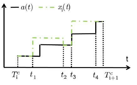
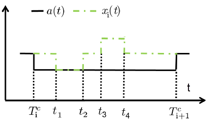
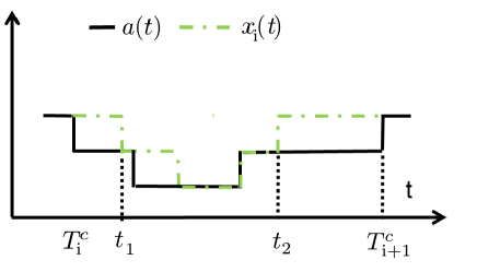
The workload in any critical segment must be one of the following four types:
-
•
Type-I: workload is non-decreasing in .
-
•
Type-II: workload is step-decreasing in . That is, and .
-
•
Type-III: workload is of “U-shape” in . That is, and .
-
•
Type-IV: workload is of “canyon-shape” in . That is, , and not always identical, .
Proof:
Refer to Appendix -A. ∎
Examples of these four types of are shown in Fig. 1.
III-B Structure of Optimal Solution
Let , , be an optimal solution to the problem SCP, and the corresponding minimum server operation cost be . We have the following observation.
Lemma 2.
must meet at every critical time, i.e., , .
Proof:
Refer to Appendix -B. ∎
Lemma 2 not only presents a necessary condition for a solution to be optimal, but also suggests a “divide-and-conquer” way to solve the problem SCP optimally.
Consider the following sub-problem of minimizing server operation cost in a critical segment , :
| min | (7) | ||||
| (9) | |||||
| var | (10) |
Let its optimal value be , . We have the following observation.
Lemma 3.
is a lower bound of the optimal server operation cost of the problem SCP, i.e.,
| (11) |
Proof:
Refer to Appendix -C. ∎
Remark: Over arbitrarily chopped segments, sum of their minimum server operation costs may not be bounds for . However, as we will see later, computed based on critical segments, Eqn. (11) establishes a lower bound of and is achievable, thanks to the structure of outlined in Lemma 2.
Suggested by Lemma 3, it suffices to solve
individual sub-problems for all critical segments in , and
combine the corresponding solutions to form an optimal solution to
the overall problem SCP (note the optimal solutions of sub-problems
connect seamlessly). The special structures of in individual
critical segment, summarized in Proposition 1,
are the key to tackle each sub-problem.
Optimal Solution Construction Procedure:
We visit all the critical segments in sequentially, and construct an , . For a critical segment , , we check the in it:
-
1.
the is of Type-I or Type-II: we simply set , for all .
-
2.
the is of Type-III:
-
•
if , then we set ;
-
•
otherwise, we set , , and .
-
•
-
3.
the is of Type-IV:
-
•
if , then we set ;
-
•
Otherwise, we construct as follows. In Type-IV critical segment, each job-departure epoch in has a corresponding job-arrival epoch in such that and . Finding the first job-departure epoch after in who has a corresponding job-arrival epoch such that . Then finding the first job-departure epoch after who has a corresponding job-arrival epoch such that . Go on this way until we reach . Upon reaching time epoch , we find all, say , such job-departure and arrival epoch pairs ,…. If , which means there does not exist such job-departure and arrival epoch pair, we set , otherwise, we set and for .
-
•
The following theorem shows that the lower bound of in (11) is achieved by using the above procedure.
Theorem 4.
The Optimal Solution Construction Procedure terminates in finite time, and the resulting , , is an optimal solution to the problem SCP.
Proof:
Refer to Appendix -D. ∎
The proof utilizes proof-by-contradiction and counting arguments.
III-C Intuitions and Observations
Constructing optimal for critical segments with Type-I/II/III workload is rather straightforward. In the following, we go through the construction of for the critical segment with Type-IV workload shown in Fig. 2, to bring out the intuition. We define
| (12) |
as the critical interval over which the energy cost of maintaining an idle server matches the cost of turning it off at the beginning of the interval and turning it on at the end of the interval.

During the critical segment with Type-IV workload shown in Fig. 2, the system starts and ends with 2 jobs and 2 running servers. Let the servers with their jobs leaving at time and be S1 and S2, respectively.
At time , a job leaves. The procedure compares and . If , then it sets and keeps all two servers running for all ; otherwise, it further applies the Critical Segment Construction Procedure and decomposes the critical segment into three small ones , , and , as shown in Fig. 2. The first small critical segment has a Type-II workload, thus the procedure sets for . The second small segment has a Type-III workload; thus for all , the procedure maintains if and sets otherwise. The last small segment has a Type-I workload, thus the procedure set for and .
These actions reveal two important observations, upon which we build a decentralized off-line algorithm to solve the problem SCP optimally.
-
•
Newly arrived jobs should be assigned to servers in the reverse order of their last-empty-epochs.
In the example, when a new job arrives at time , the procedure implicitly assigns it to server S2 instead of S1. As a result, S1 and S2 have empty periods of and , respectively. This may sound counter-intuitive as compared to an alternative “fair” strategy that assigns the job to the early-emptied server S1, which gives S1 and S2 empty periods of and , respectively. Different job-dispatching gives different empty-period distribution. It turns out a more skew empty-period distribution leads to more energy saving.
The intuition is that job-dispatching should try to make every server empty as long as possible so that the on-off option, if explored, can save abundant energy.
-
•
Upon being assigned an empty period, a server only needs to independently make locally energy-optimal decision.
It is straightforward to verify that in the example, upon a job leaving server S1 at time , the procedure implicitly assigns an empty-period of to S1, and turns S1 off if and keeps it running at idle state otherwise. Similarly, upon a job leaving S2 at time , S2 is turned off if and stays idle otherwise. Such comparisons and decisions can be done by individual servers themselves.
III-D Offline Algorithm Achieving the Optimal Solution
The Optimal Solution Construction Procedure determines how many running servers to maintain at time , i.e., , to achieve the optimal server operation cost . However, as discussed in Section II-A, under the continuous-time brick model, scheduling servers on/off according to might incur non-trivial job migration cost.
Exploiting the two observations made in the case-study at the end
of last subsection, we design a simple and decentralized off-line
algorithm that gives an optimal and incurs no job
migration cost.
Decentralized Off-line Algorithm A0:
By a central job-dispatching entity: it implements a last-empty-server-first strategy. In particular, it maintains a stack (i.e., a Last-In/First-Out queue) storing the IDs for all idle or off servers. Before time , the stack contains IDs for all the servers that are not serving.
-
•
Upon a job arrival: the entity pops a server ID from the top of the stack, and assigns the job to the corresponding server (if the server is off, the entity turns it on).
-
•
Upon a job departure: a server just turns idle, the entity pushes the server ID into the stack.
By each server:
-
•
Upon receiving a job: the server starts serving the job immediately.
-
•
Upon a job leaving this server and it becomes empty: let the current time be . The server searches for the earliest time so that . If no such exists, then the server turns itself off. Otherwise, it stays idle.
We remark that in the algorithm, we use the same server to serve a job during its entire sojourn time. Thus there is no job migration cost. The following theorem justifies the optimality of the off-line algorithm.
Theorem 5.
The proposed off-line algorithm A0 achieves the optimal server operation cost of the problem SCP.
Proof:
Refer to Appendix -E. ∎
There are two important observations. First, the job-dispatching strategy only depends on the past job arrivals and departures. Consequently, the strategy assigns a job to the same server no matter it knows future job arrival/departure or not; it also acts independently to servers’ off-or-idle decisions. Second, each individual server is actually solving a classic ski-rental problem [24] – whether to “rent”, i.e., keep idle, or to “buy”, i.e., turn off now and on later, but with their “days-of-skiing” (corresponding to servers’ empty periods) jointly determined by the job-dispatching strategy.
Next, we exploit these two observations to extend the off-line algorithm A0 to its online versions with performance guarantee.
IV Online Dynamic Provisioning with or without Future Workload Information
Inspired by our off-line algorithm, we construct online algorithms by combining (i) the same last-empty-server-first job-dispatching strategy as the one in algorithm A0, and (ii) an off-or-idle decision module running on each server to solve an online ski-rental problem.
As discussed at the end of last section, the last-empty-server-first job-dispatching strategy utilizes only past job arrival/departure information. Consequently, as compared to the offline case, in the online case it assigns the same set of jobs to the same server at the same sequence of epochs. The following lemma rigorously confirms this observation.
Lemma 6.
For the same , under the last-empty-server-first job-dispatching strategy, each server will get the same job at the same time and the job will leave the server at the same time for both off-line and online situations.
Proof:
Refer to Appendix -F. ∎
As a result, in the online case, each server still faces the same set of off-or-idle problems as compared to the off-line case. This is the key to derive the competitive ratios of our to-be-presented online algorithms.
Each server, not knowing the empty periods ahead of time, however, needs to decide whether to stay idle or be off (and if so when) in an online fashion. One natural approach is to adopt classic algorithms for the online ski-rental problem.
IV-A Dynamic Provisioning without Future Workload Information
For the online ski-rental problem, the break-even algorithm in [24] and the randomized algorithm in [25] have competitive ratios and , respectively. The ratios have been proved to be optimal for deterministic and randomized algorithms, respectively. Directly adopting these algorithms in the off-or-idle decision module leads to two online solutions for the problem SCP with competitive ratios and . These ratios improve the best known ratio achieved by the algorithm in [20].
The resulting solutions are decentralized and easy to implement: a central entity runs the last-empty-server-first job-dispatching strategy, and each server independently runs an online ski-rental algorithms. For example, if the break-even algorithm is used, a server that just becomes empty at time will stay idle for amount of time. If it receives no job during this period, it turns itself off. Otherwise, it starts to serve the job immediately. As a special case covered by Theorem 7, it turns out this directly gives a -competitive dynamic provisioning solution.
IV-B Dynamic Provisioning with Future Workload Information
Classic online problem studies usually assume zero future information. However, in our data center dynamic provisioning problem, one key observation many existing solutions exploited is that the workload expressed highly regular patterns. Thus the workload information in a near prediction window may be accurately estimated by machine learning or model fitting based on historical data [14, 26]. Can we exploit such future knowledge, if available, in designing online algorithms? If so, how much gain can we get?
Let’s elaborate through an example to explain why and how much future knowledge can help. Suppose at any time , the workload information in a prediction window is available, where is a constant. Consider a server running the break-even algorithm just becomes empty at time , and its empty period happens to be just a bit longer than .
Following the standard break-even algorithm, the server waits for amount of time before turning itself off. According to the setting, it receives a job right after epoch, and it has to power up to serve the job. This incurs a total cost of as compared to the optimal one , which is achieved by the server staying idle all the way.
An alternative strategy that costs less is as follows. The server stays idle for amount of time, and peeks into the prediction window . Due to the last-empty-server-first job-dispatching strategy, the server can easy tell that it will receive a job if any in the window exceeds , and no job otherwise. According to the setting, the server sees itself receiving no job during and it turns itself off at time . Later it turns itself on to serve the job right after . Under this strategy, the overall cost is and is better than that of the break-even algorithm.
This simple example shows it is possible to modify classic online algorithms to exploit future workload information to obtain better performance. To this end, we propose new future-aware online ski-rental algorithms and build new online solutions.
We model the availability of future workload information as follows. For any , the workload for in the window is known, where is a constant and represents the size of the window.
We present both the modified break-even algorithm and the resulting decentralized and deterministic online solution as follow. The modified future-aware break-even algorithm is very simple and is summarized as the part in the server’s actions upon job departure.
Future-Aware Online Algorithm A1:
By a central job-dispatching entity: it implements the last-empty-server-first job-dispatching strategy, i.e., the one described in the off-line algorithm.
By each server:
-
•
Upon receiving a job: the server starts serving the job immediately.
-
•
Upon a job leaving this server and it becomes empty: the server waits for amount of time,
-
–
if it receives a job during the period, it starts serving the job immediately;
-
–
otherwise, it looks into the prediction window of size . It turns itself off, if it will receive no job during the window. Otherwise, it stays idle.
-
–
In fact, as shown in Theorem 7 later in this section, the algorithm A1 has the best possible competitive ratio for any deterministic algorithms under the last-empty-server-first job-dispatching strategy. Thus, unless we change the job-dispatching strategy, no deterministic algorithms can achieve better competitive ratio than the algorithm A1.
Similarly, we present both the modified randomized algorithms for solving online ski-rental problem and the resulting decentralized and randomized online solutions as follow. The modified future-aware randomized algorithms are also summarized as the part in the server’s actions upon job departure. The first randomized algorithm A2 is a direct extension of the one in [25] to make it future-aware. The algorithm A3 is new and it has the best possible competitive ratio for any randmonized algorithms under the last-empty-server-first job-dispatching strategy.
Future-Aware Online Algorithm A2:
By a central job-dispatching entity: it implements the last-empty-server-first job-dispatching strategy, i.e., the one described in the off-line algorithm.
By each server:
-
•
Upon receiving a job: the server starts serving the job immediately.
-
•
Upon a job leaving this server and it turns empty: the server waits for amount of time, where is generated according to the following probability density function
-
–
if it receives a job during the period, it starts serving the job immediately;
-
–
otherwise, it looks into the prediction window of size . It turns itself off, if it will receive no job during the window. Otherwise, it stays idle.
-
–
Future-Aware Online Algorithm A3:
By a central job-dispatching entity: it implements the last-empty-server-first job-dispatching strategy, i.e., the one described in the off-line algorithm.
By each server:
-
•
Upon receiving a job: the server starts serving the job immediately.
-
•
Upon a job leaving this server and it turns empty: the server waits for amount of time, where is generated according to the following probability distribution
-
–
if it receives a job during the period, it starts serving the job immediately;
-
–
otherwise, it looks into the prediction window of size . It turns itself off, if it will receive no job during the window. Otherwise, it stays idle.
-
–
The three future-aware online algorithms inherit the nice properties of the proposed off-line algorithm in the previous section. The same server is used to serve a job during its entire sojourn time. Thus there is no job migration cost. The algorithms are decentralized, making them easy to implement and scale.
Observing no such future-aware online algorithms available in the literature, we analyze their competitive ratios and present the results as follows.
Theorem 7.
The deterministic online algorithm A1 has a competitive ratio of . The randomized online algorithm A2 achieves a competitive ratio of . The randomized online algorithm A3 achieves a competitive ratio of . The competitive ratios of the algorithms A1 and are A3 the best possible for deterministic and randomized algorithms, respectively, under the last-empty-server-first job-dispatching strategy.
Proof:
Refer to Appendix -F. ∎
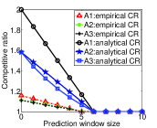
Remarks: (i) When , all three algorithms achieve the optimal server operation cost. This matches the intuition that servers only need to look amount of time ahead to make optimal off-or-idle decision upon job departures. This immediately gives a fundamental insight that future workload information beyond the critical interval (corresponding to ) will not improve dynamic provisioning performance. (ii) The competitive ratios presented in the above theorem is for the worst case. We have carried out simulations using real-world traces and found the empirical ratios are much better, as shown in Fig. 3. (iii) To achieve better competitive ratios, the theorem says that it is necessary to change the job-dispatching strategy, since otherwise no deterministic or randomized algorithms do better than the algorithms A1 and A3. (iv) Our analysis assumes the workload information in the prediction window is accurate. We evaluate the two online algorithms in simulations using real-world traces with prediction errors, and observe they are fairly robust to the errors. More details are provided in Section V.
IV-C Adapting the Algorithms to Work with Discrete-Time Fluid Workload Model
Adapting our off-line and online algorithms to work with the discrete-time fluid workload model involves two simple modifications. Recall in the discrete-time fluid model, time is chopped into equal-length slots. Jobs arriving in one slot get served in the same slot. Workload can be split among running servers at arbitrary granularity like fluid.
For the job-dispatching entity in all the algorithms, at the end of each slot when all servers are considered to be empty, it pushes all the server IDs back into the stack (order doesn’t matter). Then at the beginning of each slot, it pops just-enough server IDs from the stack in a Last-In/First-Out manner to satisfy the current workload. In this way, the job-dispatching entity essentially packs the workload to as few servers as possible, following the last-empty-server-first strategy.
For individual servers, they start to serve upon receiving jobs, and start to solve the off-line or online ski-rental problems upon all its jobs leaving and it becomes empty.
It is not difficult to verify the modified algorithms still retain their corresponding performance guarantees. Actually, we have following corollary.
Corollary 8.
The modified deterministic and randomized online algorithms for discrete-time fluid workload have competitive ratios of , , and , respectively.
Proof:
Refer to Appendix -G. ∎
IV-D Comparison with the DELAYEDOFF Algorithm
It is somewhat surprising to find out our algorithms share similar ingredients as the DELAYEDOFF algorithm in [22], since these are two independent efforts setting off to optimize different objective functions (total energy consumption in our study v.s. Energy-Response time Product (ERP) in [22]).
The DELAYEDOFF algorithm contains two modules. The first one is a job-dispatching module that assigns a newly arrived job to the most-recently-busy idle server (i.e., the idle server who was most recently busy); servers in off-state are not included. The second one is a delay-off module running on each server that keeps the server idle for some pre-determined amount of time, defined as , before turning it off. If the server gets a job to service in this period, its idle time is reset to . The authors of [22] show that for any , if the job arrival process is Poisson, the DELAYEDOFF algorithm minimizes the average ERP of a data center as the load (i.e., the ratio between the arrival rate and the average sojourn time) approaches infinity.
Interestingly, if there are idle servers in system, DELAYEDOFF and the algorithm A1 will choose the same server to serve the new job because the most-recently-busy server is indeed the last-empty server in this case. If there are no idle servers, the algorithm A1 will still choose the last-empty server but DELAYEDOFF will randomly select an off server to server the job. With this observation, the DELAYEDOFF algorithm, under the setting , can be viewed as a variant of a special case of the algorithm A1 with zero future workload information available (i.e., ). It would be interesting to see whether the analytical insights used in analyzing the DELAYEDOFF algorithm can be used to understand the performance of the algorithm A1 when the job arrival process is Poisson.
Despite the similarity between the algorithm A1 and the DELAYEDOFF algorithm, it is not clear what is the competitive ratio of DELAYEDOFF. Unlink our last-empty-server-first job-dispatching strategy, the most-recently-busy idle server first strategy does not guarantee a server faces the same set of ski-rental problems in the online case as compared to the off-line case. Consequently, it is not clear how to relate the online cost of the DELAYEDOFF algorithm to the offline optimal cost.
The two job-dispatching strategies differ more when the server waiting time is random, e.g., in our algorithms A2 and A3, where a later-empty server may turn itself off before an early-empty server does; hence, the most-recently-busy (idle) server is usually not the last-empty server. We compare the performance of algorithms A1, A2, A3, and DELAYEDOFF in simulations in Section V.
V Experiments
We implement the proposed off-line and online algorithms and carry out simulations using real-world traces to evaluate their performance. Our purposes are threefold. First, to evaluate the performance of the algorithms using real-world traces. Second, to study the impacts of workload prediction error and workload characteristic on the algorithms’ performance. Third, to compare our algorithms to two recently proposed solutions LCP) in [20] and DELAYEDOFF in [22].
V-A Settings
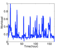
Workload trace: The real-world traces we use in experiments are a set of I/O traces taken from 6 RAID volumes at MSR Cambridge [27]. The traced period was one week between February 22 to 29, 2007. We estimate the average number of jobs over disjoint 10 minute intervals. The data trace has a peak-to-mean ratio (PMR) of 4.63. The jobs are “request-response” type and thus the workload is better described by a discrete-time fluid model, with the slot length being 10 minutes and the load in each slot being the average number of jobs.
As discussed in Section IV-C, the proposed off-line and online algorithms also work with the discrete-time fluid workload model after simple modification. In the experiments, we run the modified algorithms using the above real-world traces.
Cost benchmark: Current data centers usually do not use dynamic provisioning. The cost incurred by static provisioning is usually considered as benchmark to evaluate new algorithms [20, 15]. Static provisioning runs a constant number of servers to serve the workload. In order to satisfy the time-varying demand during a period, data centers usually overly provision and keep more running servers than what is needed to satisfy the peak load. In our experiment, we assume that the data center has the complete workload information ahead of time and provisions exactly to satisfy the peak load. Using such benchmark gives us a conservative estimate of the cost saving from our algorithms.
Sever operation cost: The server operation cost is determined by unit-time energy cost and on-off costs and . In the experiment, we assume that a server consumes one unit energy for per unit time, i.e., . We set , i.e., the cost of turning a server off and on once is equal to that of running it for six units of time [20]. Under this setting, the critical interval is units of time.
V-B Performance of the Proposed Online Algorithms
We have characterized in Theorem 7 the competitive ratios of our proposed online algorithms as the prediction window size, i.e., , increases. The resulting competitive ratios, i.e., , and , already appealing, are for the worst-case scenarios. In practice, the actual performance can be even better.
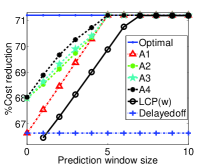
In our first experiment, we study the performance of our online algorithms using real-world traces. The results are shown in Fig. 4b. The cost reduction curves are obtained by comparing the power cost incurred by the off-line algorithm, the three online algorithms, the LCP algorithm [20] and the DELAYEDOFF algorithm [22] to the cost benchmark. The vertical axis indicates the cost reduction and the horizontal axis indicates the size of prediction window varying from 0 to 10 units of time.
As seen, for this set of workload, both our three online algorithms, LCP and DELAYEDOFF achieve substantial cost reduction as compared to the benchmark. In particular, the cost reductions of our three online algorithms are beyond even when no future workload information is available; while LCP has to have (or estimate) one unit time of future workload to execute, and thus it starts to perform when the prediction window size is one. The cost reductions of our three online algorithms grow linearly as the prediction window increases, and reaching optimal when the prediction window size reaches . These observations match what Theorem 7 predicts. Meanwhile, LCP has not yet reach the optimal performance when the prediction window size reaches the critical value . DELAYEDOFF has the same performance for all prediction window sizes since it does not exploit future workload information.
As seen in Fig. 4b, in the simulation, our three algorithms can achieve the optimal power consumption when the size of prediction window is , one unit smaller than the theoretically-computed one . At first glance, the results seem not aligned with what the analysis suggests. But a careful investigation reveals that there is no mis-alignment between analysis and simulation. Because jobs are assigned to servers at the beginning of each slots in discrete-time fluid model, knowing the workload from current time to the beginning of the 5th look-ahead future slot is equivalent to knowing the workload of a duration of 6 slots. Hence, the anaysis indeed suggests Algorithms A1-A3 can achieve optimal power consumption when the size of prediction window is , as observed in Fig. 4b.
V-C Impact of Prediction Error
Previous experiments show that both our algorithms and LCP have better performance if accurate future workload is available. However, there are always prediction errors in practice. Therefore, it is important to evaluate the performance of the algorithms in the present of prediction error.
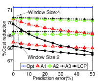
To achieve this goal, we evaluate our online algorithms with prediction window size of 2 and 4 units of time. Zero-mean Gaussian prediction error is added to each unit-time workload in the prediction window, with its standard deviation grows from to of the corresponding actual workload. In practice, prediction error tends to be small [28]; thus we are essentially stress-testing the algorithms.
We average 100 runs for each algorithm and show the results in Fig. 4c, where the vertical axis represents the cost reduction as compared to the benchmark.
On one hand, we observe all algorithms are fairly robust to prediction errors. On the other hand, all algorithms achieve better performance with prediction window size 4 than size 2. This indicates more future workload information, even inaccurate, is still useful in boosting the performance.
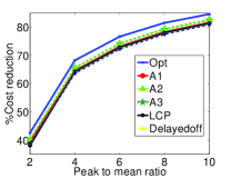
V-D Impact of Peak-to-Mean Ratio (PMR)
Intuitively, comparing to static provisioning, dynamic provisioning can save more power when the data center trace has large PMR. Our experiments confirm this intuition which is also observed in other works [20, 15]. Similar to [20], we generate the workload from the MSR traces by scaling as , and adjusting and to keep the mean constant. We run the off-line algorithm, the three online algorithms, LCP and DELAYEDOFF using workloads with different PMRs ranging from 2 to 10, with prediction window size of one unit time. The results are shown in Fig. 4d.
As seen, energy saving increases form about at PRM=2, which is common in large data centers, to large values for the higher PMRs that is common in small to medium sized data centers. Similar results are observed for different prediction window sizes.
VI Concluding Remarks
Dynamic provisioning is an effective technique in reducing server energy consumption in data centers, by turning off unnecessary servers to save energy. In this paper, we design online dynamic provisioning algorithms with zero or partial future workload information available.
We reveal an elegant “divide-and-conquer” structure of the off-line dynamic provisioning problem, under the cost model that a running server consumes a fixed amount energy per unit time. Exploiting such structure, we show its optimal solution can be achieved by the data center adopting a simple last-empty-server-first job-dispatching strategy and each server independently solving a classic ski-rental problem.
We build upon this architectural insight to design two new decentralized online algorithms. One is a deterministic algorithm with competitive ratio , where is the fraction of a critical window in which future workload information is available. The size of the critical window is determined by the wear-and-tear cost and the unit-time energy cost of running a single server. The other two are randomized algorithms with competitive ratios and , respectively. and are the best competitive ratios for deterministic and randomized online algorithms under our last-empty-server-first job-dispatching strategy. Our results also lead to a fundamental observation that under the cost model that a running server consumes a fixed amount energy per unit time, future workload information beyond the critical window will not improve the dynamic provisioning performance.
Our algorithms are simple and easy to implement. Simulations using real-world traces show that our algorithms can achieve close-to-optimal energy-saving performance, and are robust to future-workload prediction errors.
Our results, together with the -competitive algorithm recently proposed by Lin et al. [20], suggest that it is possible to reduce server energy consumption significantly with zero or only partial future workload information.
An interesting and important future direction is to explore what is the best possible competitive ratio any algorithms can achieve with zero or partial future workload information. Insights along this line provides useful understanding on the benefit of knowing future workload in dynamic provisioning.
Acknowledgements
We thank Minghong Lin and Lachlan Andrew for sharing the code of their LCP algorithm, and Eno Thereska for sharing the MSR Cambridge data center traces.
-A Proof of Proposition 1
Proof:
The proof that critical segment must belong to one of the four types described in proposition 1 is based on two cases.
Case 1: is job-arrival epoch.
In this case, according to our Critical Segment Construction Procedure, is the first departure epoch after . Then workload in is non-decreasing, which means is Type-I critical segment.
Case 2: is job-departure epoch.
In this case, we have two sub-cases. First, if we can find the first arrival epoch after so that , according to Critical Segment Construction Procedure, we let . If , is Type-III critical segment. Otherwise, is Type-IV critical segment, , and not always identical, . Second, if no such exists, then we let to be the next job departure epoch, then is Type-II critical segment. in this segment is step-decreasing, which means and .
The above two cases cover all the possible situations of critical segment . And we proved that must belong to one of the four types for both cases. Hence, we proved proposition 1. ∎
-B Proof of Lemma 2
Proof:
Because at we have , which means meets at the first critical time. We will use induction to prove Lemma 2 is true for all the rest critical times. As a matter of fact, given , we claim that . We divide the situation in two cases and in each case we will prove by adopting proof-by-contradiction.
Case 1: When is Type-I, Type-III or Type-IV critical segment, which means we must have .
If , then we can find a time such that and . Define as follows: and . It is clear that satisfy the constraints of (3). Moreover, will cause more power consumption than because will consume more power to run extra servers during and both have the same power consumption for the rest of time. It is a contradiction that is an optimal solution of (3). Therefore, .
Case 2: When is Type-II critical segment, which means we must have .
If , because , then we can find a time such that and . Define as follows: and . It is clear that satisfy the constraint of (3) due to property • ‣ 1 of Type-II critical segments. Moreover, will cost more power consumption than because will consume more power to run extra servers during and both have the same power consumption for the rest of time. It is a contradiction that is an optimal solution of (3). Therefore, .
Above two cases cover all the possibility of critical segment and we proved that in both two cases. Therefore, we proved Lemma 2.∎
-C Proof of Lemma 3
-D Proof of Theorem 4
Before proving theorem 4 , we first prove following Lemma.
Define as the following optimization problem. satisfy , and . are constants which are greater than or equal to .
| min | (13) | ||||
| (15) | |||||
| var | (16) |
Lemma 9.
The necessary condition for to achieve optimal power consumption of is that .
Proof:
Let be any optimal solution to above optimization problem and does not satisfy . In order to prove the necessary condition, we divide into four cases.
.
In this case, let , then will consume at least more power to run extra servers than during . On the other hand, causes at most more wear-and-tear cost than . Because , actually cost more power than , which is a contradiction with that is an optimal solution.
such that .
In this case, let and . then it is clear that consume more power than , which is a contradiction with that is an optimal solution.
such that
In this case, let and . then it is clear that consume more power than , which is a contradiction with that is an optimal solution.
dose not satisfy above three cases.
If does not satisfy case , then there must exist time and in such that and . Let and . satisfies all the constraints of (13). It is also easy to verify that consume more power than , which is a contradiction with that is an optimal solution.
The above four cases cover all possible situation of . Therefore, we proved that the necessary condition for to be an optimal solution to (13) is that . ∎
Now we are going to prove theorem 4.
Proof:
Let denote the number of running server constructed by Optimal Solution Construction Procedure in critical segment . We will prove that is an optimal solution of (7). The proof is based on the type of critical segment .
For critical segments of Type-I and Type-II, we claim that can achieve . Let be any solution to (7) and is not always equal to during . Because is either non-decreasing or step-decreasing in Type-I and Type-II critical segments, we can find periods in such that , and . One example of such period is in Fig. 5. It is clear that cost more power than in each such period and both have the same power consumption in the rest of time during . Therefore, is an optimal solution to (7) and can achieve optimal power consumption .
It is clear that for Type-III segment according to our Optimal Solution Construction Procedure. We divide the proof of theorem 4 for Type-III critical segment in two cases.
Case 1: .
In this case, we claim that can achieve . In fact, let be any solution to (7) and is not always equal to during . We will prove that does not cost more power consumption than in .
Since is not always equal to during , we can find period such that , and . One example of such period is in Fig. 6.
We will compare the power consumed by and in based on two situations. If , then consumes more power to run extra servers than in each period . If , on one hand, costs at most more power to run one extra server than in . On the other hand, has to consume more power to turn on/off a server one time in . Since , we have . This means does not cost more power than in . Therefore, in both situations does not cost more power than in period . If there exist other periods like ,(One example is in Fig. 6) we can prove that does not cost more power than in these periods in the same way as we did for . On the other hand, and have the same power consumption in the rest of time in . It follows that does not cost more power than in , which means is an optimal solution to (7).
Case 2: .
In this case, we claim that can achieve . Because we can turn off the new idle server at and turn on the server at . In this way, we can save power consumption which is greater then the on-off cost . Thus, can achieve .
For Type-IV segment, we divide the situation in two cases in the same way as we did for Type-III segment.
Case 1: .
In this case, we claim that can achieve . The proof is similar to the proof for Type-III critical segment under the same situation . Let be any solution to (7) and is not always equal to during . We will prove that does not cost more power than in . Because is not always equal to during , we can find period such that , and . One example of such period is in Fig. 7.
First, we will compare the power consumed by and in based on two situations. If , then consumes more power to run extra servers than in period . If , which means a certain number of servers has been turned off during for certain amount of time. Denote as the total number of servers have been turned off during . On one hand, cost at most power to run extra servers in . On the other hand, has to consume power to turn on/off servers times in . Since , we have . This means does not cost more power than in . Therefore, in both situation does not cost more power than in each period . Moreover, and have the same power consumption in the rest of time in . It follows that does not cost more power than in , which means is an optimal solution to (7).
We consider Type-I, Type-II, Type-III and Type-IV segment with to be the four basic critical segments, based on which we discuss the case of Type-IV segment with .
Case 2: .
Each job-departure epoch in has a corresponding job-arrival epoch in such that and . And we can find a set of job-departure and arrival epoch pairs ,… according to the procedure in Optimal Solution Construction Procedure for Type-IV critical segment with .
In order to prove that Optimal Solution Construction Procedure constructs an optimal solution to (7) in with , we are going to prove that an optimal solution to (7) must meet at every job-departure and its corresponding job-arrival epoch if . Based on this fact, we can prove that Optimal Solution Construction Procedure constructs an optimal solution.
It is clear that if , then we must have . Otherwise, if for some , we must have because we have for job-departure and arrival epoch . On the other hand, we also must have because . This is a contradiction with previous conclusion . Hence, .
Now, we are going to prove that the necessary condition for to achieve optimal power consumption in is that must meet at every job-arrival and its corresponding job-arrival epoch if .
It is clear the necessary condition is satisfied when . On the other hand, for any job-arrival and departure epoch pair , we can always find another job-arrival and departure epoch pair covering , i.e., and . Moreover, we must also have . Because if , then we must have for some . This means for some , which is a contradiction with .
Since achieves the optimal power consumption in , then must be an optimal solution to with . It follows that must satisfy the necessary condition of problem stated in Lemma 9, hence, . Because , we must have and .
Note that according to the necessary condition, if , then must meet at every job-departure and its corresponding job-arrival epoch in .
We are ready to prove that Optimal Solution Construction Procedure constructs an optimal solution to (7) in with . We prove it based on two cases.
For all the job-arrival and departure epoch pairs , we have .
In this case, must meet at every job-departure epoch and job-arrival epoch in according to necessary condition we just proved. It is easy to verify that between two consecutive epoches (the two epoches can be one of following four cases: both are arrival epoches, both are departure epoch, the first one is arrival epoch and the other one is departure epoch, the first one is departure epoch and the other one is arrival epoch) is one of the following smaller basic critical segments: Type-I, Type-II, Type-III with . As we already proved that is an optimal solution in these smaller basic critical segments. Therefore, we must have , which is the same as the solution constructed by our Optimal Solution Construction Procedure. Hence, can achieve optimal power consumption in .
There exist job-arrival and departure epoch pairs such that .
In this case, must meet at all job-departure epoch and job-arrival epoch which are not in . We also can verify that in two consecutive epoches which are not in is one of the following smaller basic critical segments: Type-I, Type-II, Type-III and Type-IV with . Therefore, according to the optimal solution construction procedure of the four basic critical segments, we must have when is smaller basic critical segments of Type-III with and Type-IV with . And in the rest smaller basic segments, we must have . The whole is the same as the solution constructed by our Optimal Solution Construction Procedure. Hence, can achieve optimal power consumption in .
The above two cases cover all the possibility of . We proved that in each case the solution constructed by Optimal Solution Construction Procedure can achieve the optimal. It follows that the solution constructed by Optimal Solution Construction Procedure can achieve the optimal in with .
Because we only have finite job arrival/departure in and each basic critical segment or smaller basic critical segment contains at least one job arrival or departure epoch. Therefore, the number of basic critical segments or smaller basic critical segments is finite, which means our construction can terminate in finite time.
-E Proof of Theorem 5
Proof:
First, we want to prove that the number of running servers proposed by our off-line algorithm meets at every critical time . We have . Given , we want to show that .
if is an arrival epoch, then is Type-I segment and there is no job departure during this critical segment and no idle server at . Job-dispatching entity just pops server ID and turn on corresponding server to serve new job. Thus, we have .
if is a departure epoch, then is one of the rest three types critical segments and we must have or .
When , the system only has one idle server right after . The idle server should make decision to remain idle or turn off. According to the definition of , the idle server can not find arrival epoch after so that . Based on our off-line algorithm, the server will turn itself off. Therefore, we have .
When , then the critical segment is Type-III or Type-IV segment and . Because the number of arrival epoches is less than the number of departure epoches in , which means job-dispatching entity pushed more server IDs than popped in the period . Therefore, job-dispatching entity will not pop server IDs pushed before during , which means the number of running servers during is less than or equal to . Because we have and , we must have .
By induction, we proved that meets at all the critical times.
Next, we are going to prove that and the optimal solution constructed by Optimal Solution Construction Procedure are the same. We divide the situation into four cases.
Case 1: For Type-I segment .
Because there is no job departure during the non-decreasing critical segment and we have , which means there is on idle server at . According to our off-line algorithm, job-dispatching entity just pops server ID and turns on the corresponding server when new job arriving. Thus, we have .
Case 2: For Type-II segment .
According to proposition 1, for step-decreasing segment we have . After job departure at , the new idle corresponding server can not find time so that . Hence, based on our off-line algorithm, the server turns itself off and we have .
Case 3: For Type-III segment .
For Type-III segment, job-dispatching entity will push a server ID at and pop it at If , the corresponding server can not find time so that , our off-line algorithm will turn off the corresponding server and . If , the server will remain idle and . Hence, we have .
Case 4: For Type-IV segment .
In this case, if , at each departure epoch in , the corresponding new idle server can find time so that , where is the departure epoch. Therefore, all the servers remain idle according to our off-line algorithm and . If , at each departure epoch , our offline algorithm will turn off the new idle server if the corresponding departure epoch satisfying that because the idle server can not find time so that . If , the new idle server will remain idle. In this way, the number of running servers decided by our off-line algorithm is equal to .
-F Proof of Theorem 7
Lemma 6: For the same , under the last-empty-server-first job-dispatching strategy, each server will get the same job at the same time and the job will leave the server at the same time for both off-line and online situations.
Proof:
For both off-line and online situation, we have the same servers running at . The other servers are off and their IDs are stored in the stack in the same order at . Let denote the th epoch that a job departs or arrivals the system in . Assume the number of total arrival and departure epoches is . To prove Lemma 6, we first claim that same server IDs are stored in the stack in the same order for both off-line and online situation in each period . Moreover, both situations have the same servers running and each running server serve the same corresponding job in . We will prove the claim by induction.
First, we prove that the claim is true for . If is a job-arrival epoch, for both off-line situation and online situation, the job-dispatching entity will pop the same server ID to server the new job because both off-line and online situation have the same server IDs in stack and IDs are in the same order at . After popping the server ID at the top of the stack at , both off-line and online situation still have the same server IDs stored in the stack and IDs are in the same order. And both situations have the same servers running and each running server serve the same job. Because there is no job arrival or departure in , therefore, no server ID will be popped out of the stack or pushed in the stack during , which means both the two situations will remain having the same server IDs stored in the stack in the same order and having the same servers running. Moreover, each running server serve the same corresponding job during in both two situations.
If is a job-departure epoch, for both off-line situation and online situation, the job-dispatching entity will push the same server ID in the stack because both off-line and online situation have the same servers serving the same jobs at . After pushing the server ID in the stack at , both off-line and online situation still have the same server IDs stored in the stack and IDs are in the same order, Moreover, both situations have the same servers running and each running server serve the same job. Because there is no job arrival or departure in , both the two situations will remain having the same server IDs stored in the stack in the same order and having the same servers running and each running server serve the same job during . Therefore, the claim is true for no matter is a job-arrival or departure epoch.
Next, we will prove that same server IDs are stored in the stack in the same order for both off-line and online situation in period , Moreover, both off-line and online situation have the same serving running and each running server serve the same job in two situations in period , given that both the two situations have the same server IDs stored in the stack in the same order and both off-line and online situation have the same serving running and each running server serve the same job in two situations in . The proof is also based on two cases. If is a job-arrival epoch, for both off-line situation and online situation, the job-dispatching entity will pop the same server ID to server the new job because both off-line and online situation have the same server IDs in stack and IDs are in the same order in . After popping the server ID at the top of the stack at , both off-line and online situation still have the same server IDs stored in the stack and IDs are in the same order. They also have the same running servers and each server server the same job due to both the situation have the same servers running and each server serve the same job in . Because there is no job arrival or departure in , therefore, no server ID will be popped out of the stack or pushed in the stack during , which means both the two situations will remain having the same server IDs stored in the stack in the same order and having the same servers running and each running server serve the same job during .
If is a job-departure epoch, for both off-line situation and online situation, the job-dispatching entity will push the same server ID in the stack because both off-line and online situation have the same servers serving the same jobs in . After pushing the server ID in the stack at , both off-line and online situation still have the same server IDs stored in the stack and IDs are in the same order. Moreover, They also have the same running servers and each server server the same job due to both the situation have the same servers running and each server serve the same job in . Because there is no job arrival or departure in , both the two situations will remain having the same server IDs stored in the stack in the same order and having the same servers running and each running server serve the same job during . Therefore, the claim is true for no matter is a job-arrival or departure epoch.
Up to now, we proved that same server IDs are stored in the stack in the same order for both off-line and online situation in each period . Moreover, both situations have the same servers running and each running server serve the same job in . Due to this fact, we can prove Lemma 6. If a server get a job at a job-arrival epoch in online situation, then same server will get the same job at the job-arrival epoch in off-line situation because both the situation have same server IDs stored on the top of the stack. On the other hand, if a job leave a server in online situation, then the same job will leave the same server because both situation have the same running server to serve the same job.∎
Lemma 10.
The deterministic online ski-rental algorithm we applied in our online algorithm A1 has competitive ratio .
Proof:
As we already proved in Lemma 6, for both online and off-line cases, a server faces the same set of jobs. From now on, we focus on one server. Job-dispatching entity will assign job to the server form time to time and we assume that the server will serve total jobs in . Denote as the time in that the server gets its th job and define as the time that th job of the server leaves the system. Define . The server should decide to turn off itself of stay idle between and . In order to get competitive ratio of the deterministic online ski-rental algorithm we applied in A1, we want to compare the power consumption of the online ski-rental algorithm in with the power consumption of off-line ski-rental algorithm in . In fact, the power consumption of the online and off-line ski-rental algorithms depend on the length of the time between and . Denote as the length of busy period in and as the length of empty period in , then we have:
| (17) |
According to the online ski-rental algorithm in A1, we also have:
| (18) |
Hence, when , , when
In the above calculation, we used and we have for any . On the other hand, for any , we have . Therefore, the power consumption of the online ski-rental algorithm in is at most times the optimal, which means the competitive ratio of the deterministic online ski-rental algorithm applied in A1 is . ∎
Lemma 11.
The randomized online ski-rental algorithm we applied in our online algorithm A2 has competitive ratio .
Proof:
In the proof, we still focus on one server. we will use the same notations we used to prove Lemma 10. We want to compare the average power consumption of the randomized online ski-rental algorithm in with power consumption of off-line ski-rental algorithm in . we have:
| (19) |
And according to the randomized online ski-rental algorithm, when , we have
When , we have
When we have
We get the above expected power consumption for based on following reason: If the number generated by the server is less than , then the server will waits for amount of time, consuming power. And it looks into the prediction window of size and find it won’t receive any job during the window because . Therefore, it turns itself off and cost power . On the other hand, if , the server will not turn itself off and consume to stay idle. We can get the expected power consumption for and in the same way. Because
We can calculate and the ratio between and :
From above expression, we can conclude that for any . On the other hand, for any , we have . Therefore, the power consumption of the online ski-rental algorithm in is at most times the optimal, which means the competitive ratio of the randomized online ski-rental algorithm applied in A2 is . ∎
Lemma 12.
The randomized online ski-rental algorithm we applied in our online algorithm A3 has competitive ratio .
Proof:
Now we are ready to prove theorem 7.
Proof:
As we already proved in our off-line algorithm that the optimal power consumption of the data center can be achieved by each server run off-line ski-rental algorithm individually and independently. On the other hand, in Lemma 10, 11 and 12, we proved that the power consumption of deterministic and randomized online ski-rental algorithm we applied are at most , and times the power consumption of off-line ski-rental algorithm for one server. Therefore, the power consumption of our online algorithm A1, A2 and A3 are at most , and times the power consumption of off-line algorithm for data center, which means the competitive ratios of A1, A2 and A3 are , and respectively.
Next, we want to prove that A1 has the best competitive ratio for deterministic online algorithms under our job-dispatching strategy. In fact, assume that deterministic online algorithm peeks into the future window and then decide to turn off itself or stay idle after becoming empty at . When , if the server will receive its next job right after , then the online algorithm will turn off itself at , and consume power. On the other hand, the offline optimal is . The competitive ratio is at least .
When , if the server will receive its next job right after , then the online algorithm will turn off itself at , and consume power. On the other hand, the offline optimal is . The competitive ratio at least is .
Based on above two cases, we can see that only when , the deterministic algorithm has better competitive ratio . Therefore, the best deterministic online algorithm is A1, which has competitive ratio .
Finally, we want to prove that A3 has the best competitive ratio for randomized online algorithms under our job-dispatching strategy. In fact, assume that the server becomes empty at and it will receive its next job at . In order to find the best competitive ratio for randomized online algorithm, according to the proof of Lemma 11, it is sufficient to find the minimal ratio of the power consumed by randomized online algorithm to that of the offline optimal in . We first chop time period into small time slot. Then we let the length of slot goes to zero, we can get the best competitive ratio for continuous time randomized online algorithm.
Assume critical interval contains exact slots and there are slots in . Moreover, the future window has slots. (If , the online algorithm can achieve the offline optimal and the competitive ratio is 1.) Let denote the probability that the algorithm decides to turn off the server at slot . Define as the competitive ratio. Then we can solve following optimization problem to find the minimal competitive ratio.
| (20) | |||||
| (24) | |||||
| var | (25) |
We are going to prove that the optimal value of problem (20) is equal to the optimal value of following problem.
| min | (26) | ||||
| (30) | |||||
| var | (31) |
On the other hand, let be an optimal solution to achieve in (20). If , then and satisfy the constraints of (26), which means .
If there exists , such that . Then we can prove that and satisfy the constraints of (26). In fact, when , It is easy to verify that the coefficient of is equal to the coefficient of in each constraint of (20). Therefore, and satisfy the constraints of (26).
Since when in (20), then we have
| (32) |
It is easy to verify that the coefficient of is equal to or greater than the coefficient of . Therefore, when , and still satisfy the constraints of (26) due to (32).
Hence, in both cases, and satisfy the constraints of (26), we must have . Since we already proved that , we must have .
Next, we are going to prove that an optimal solution to (26) must satisfy that .
First, if , let be the minimal such that . Then it can be verified that the constraints of (26) must hold as strict inequality for .
On the other hand, the coefficient of must be less than that of in the constraints for . Therefore, we can decrease a little bit and increase a little bit such that all the constraints of (26) have slackness, which means we can find a smaller which satisfies all the constraints. This is a contradiction that is an optimal solution. Therefore, we must have .
Second, if there exists such that , then we can decrease a little bit and increase a little bit. Since the coefficient of must greater than or equal to that of in the constraints for . On the other hand, when , we want to compare the following constraints of and .
When , it is clear that the coefficient of is at most greater than the coefficient of . Therefore, when we decrease a little bit and increase a little bit, the left side of those constraints increase at most comparing to the case . However, the right side increase at least . Hence, after we decreasing a little bit and increasing a little bit, all the constraints of (26) have slackness, which means we can find a smaller . This is a contradiction that is an optimal solution. Therefore, . Up to now, we proved that an optimal solution to (26) must satisfy that .
Because (26) is a linear optimization problem and the optimal value is not negative infinity, an optimal solution must be a vertex of the polyhedron. Moreover, we have . Hence, the constraints can not be active. On the other hand, the dimension of variable vector is equal to the number of the left independent constraints in (26). Therefore, an optimal solution must be the vertex that makes all the constraints which are not active, which means all the inequalities must hold as equalities.
We can solve the linear equation system and get the minimal competitive ratio and probability distribution:
Let go to infinity and , we have
This means the minimal competitive ratio for continuous time randomized online algorithm is .
Therefore, we proved Theorem 7.∎
-G Proof of Corollary 8
Proof:
As we already showed before, under our last-empty-server-first job dispatching strategy, each server actually serve the same set of job both in online or offline situation. Moreover, the power consumption of data center is minimal if each server runs off-line ski-rental algorithm individually and independently in off-line situation. Therefore, if each server runs online ski-rental algorithm individually and independently in online situation, assume the competitive ratio of the online ski-rental algorithm is , then the total power consumption is at most the minimal power consumption times .
However, we must apply discrete time online ski-rental algorithm for discrete-time fluid workload model because we chopped time into equal-length slots. According to [29], the competitive ratio of discrete time online ski-rental algorithm is less than or equal to that of continuous time online ski-rental problem. Therefore, our modified deterministic and randomize online algorithms can retain competitive ratios , and , where is the ratio of the number of time slots in future window to the number of slots in critical interval .∎
References
- [1] J. G. Koomey, “Worldwide electricity used in data centers,” Environmental Research Letters, no. 3, 2008.
- [2] I. E. Agency, “World energy balances (2007 edition),” 2007.
- [3] L. Barroso, “The price of performance,” ACM Queue, vol. 3, no. 7, pp. 48–53, 2005.
- [4] U.S. Environmental Protection Agency, “Epa report on server and data center energy efficiency,” ENERGY STAR Program, 2007.
- [5] Z. Liu, M. Lin, A. Wierman, S. Low, and L. Andrew, “Greening geographical load balancing,” in Proc. ACM SIGMETRICS, 2011, pp. 233–244.
- [6] P. Wendell, J. Jiang, M. Freedman, and J. Rexford, “Donar: decentralized server selection for cloud services,” in Proc. ACM SIGCOMM, vol. 40, no. 4, 2010, pp. 231–242.
- [7] A. Qureshi, R. Weber, H. Balakrishnan, J. Guttag, and B. Maggs, “Cutting the electric bill for internet-scale systems,” in Proc. ACM SIGCOMM, 2009, pp. 123–134.
- [8] R. Urgaonkar, B. Urgaonkar, M. Neely, and A. Sivasubramaniam, “Optimal power cost management using stored energy in data centers,” in Proc. ACM SIGMETRICS, 2011, pp. 221–232.
- [9] N. Rasmussen, “Electrical efficiency modeling of data centers,” Technical Report White Paper, vol. 113.
- [10] R. Sharma, C. Bash, C. Patel, R. Friedrich, and J. Chase, “Balance of power: Dynamic thermal management for internet data centers,” IEEE Internet Computing, 2005.
- [11] R. Raghavendra, P. Ranganathan, V. Talwar, Z. Wang, and X. Zhu, “No power struggles: Coordinated multi-level power management for the data center,” in ACM SIGARCH Computer Architecture News, vol. 36, no. 1, 2008, pp. 48–59.
- [12] J. Chase, D. Anderson, P. Thakar, A. Vahdat, and R. Doyle, “Managing energy and server resources in hosting centers,” in Proc. ACM SOSP, 2001.
- [13] E. Pinheiro, R. Bianchini, E. Carrera, and T. Heath, “Load balancing and unbalancing for power and performance in cluster-based systems,” in Workshop on Compilers and Operating Systems for Low Power, 2001.
- [14] G. Chen, W. He, J. Liu, S. Nath, L. Rigas, L. Xiao, and F. Zhao, “Energy-aware server provisioning and load dispatching for connection-intensive internet services,” in Proc. USENIX NSDI, 2008.
- [15] A. Krioukov, P. Mohan, S. Alspaugh, L. Keys, D. Culler, and R. Katz, “Napsac: design and implementation of a power-proportional web cluster,” ACM SIGCOMM Computer Communication Review, vol. 41, no. 1, pp. 102–108, 2011.
- [16] X. Fan, W. Weber, and L. Barroso, “Power provisioning for a warehouse-sized computer,” in Proc. the 34th annual international symposium on Computer architecture, 2007.
- [17] L. Barroso and U. Holzle, “The case for energy-proportional computing,” IEEE Computer, vol. 40, no. 12, pp. 33–37, 2007.
- [18] D. Meisner, B. Gold, and T. Wenisch, “Powernap: eliminating server idle power,” ACM SIGPLAN Notices, 2009.
- [19] H. Qian and D. Medhi, “Server operational cost optimization for cloud computing service providers over a time horizon,” in Proceedings of the 11th USENIX conference on Hot topics in management of internet, cloud, and enterprise networks and services, 2011, pp. 4–4.
- [20] M. Lin, A. Wierman, L. Andrew, and E. Thereska, “Dynamic right-sizing for power-proportional data centers,” Proc. IEEE INFOCOM, Shanghai, China, pp. 10–15, 2011.
- [21] A. Beloglazov, R. Buyya, Y. C. Lee, and A. Zomaya, “A taxonomy and survey of energy-efficient data centers and cloud computing systems,” Univ. of Melbourne, Tech. Rep. CLOUDS-TR-2010-3, 2010.
- [22] A. Gandhi, V. Gupta, M. Harchol-Balter, and M. Kozuch, “Optimality analysis of energy-performance trade-off for server farm management,” Performance Evaluation, 2010.
- [23] R. Doyle, J. Chase, O. Asad, W. Jin, and A. Vahdat, “Model-based resource provisioning in a web service utility,” in Proceedings of the 4th conference on USENIX Symposium on Internet Technologies and Systems, 2003.
- [24] A. Karlin, M. Manasse, L. Rudolph, and D. Sleator, “Competitive snoopy caching,” Algorithmica, vol. 3, no. 1, pp. 79–119, 1988.
- [25] A. Karlin, M. Manasse, L. McGeoch, and S. Owicki, “Competitive randomized algorithms for nonuniform problems,” Algorithmica, vol. 11, no. 6, pp. 542–571, 1994.
- [26] P. Bodík, R. Griffith, C. Sutton, A. Fox, M. Jordan, and D. Patterson, “Statistical machine learning makes automatic control practical for internet datacenters,” in Proceedings of the 2009 conference on Hot topics in cloud computing.
- [27] D. Narayanan, A. Donnelly, and A. Rowstron, “Write off-loading: Practical power management for enterprise storage,” ACM Transactions on Storage (TOS), vol. 4, no. 3, p. 10, 2008.
- [28] D. Kusic, J. Kephart, J. Hanson, N. Kandasamy, and G. Jiang, “Power and performance management of virtualized computing environments via lookahead control,” Cluster Computing, vol. 12, no. 1, pp. 1–15, 2009.
- [29] C. Mathieu, “Online algorithms:ski rental.” [Online]. Available: http://www.cs.brown.edu/~claire/Talks/skirental.pdf