Reliable a-posteriori error estimators for $hp$-adaptive finite element approximations of eigenvalue/eigenvector problems

Abstract.

We present reliable a-posteriori error estimates for $hp$-adaptive finite element approximations of eigenvalue/eigenvector problems. Starting from our earlier work on $h$ adaptive finite element approximations we show a way to obtain reliable and efficient a-posteriori estimates in the $hp$-setting. At the core of our analysis is the reduction of the problem on the analysis of the associated boundary value problem. We start from the analysis of Wohlmuth and Melenk and combine this with our a-posteriori estimation framework to obtain eigenvalue/eigenvector approximation bounds.

1. Introduction

Accurate computation of eigenvalues and eigenvectors of differential operators defined in planar regions has attracted considerable attention recently. A central paper in this body of work is the 2005 contribution of Trefethen and Betcke [7] on computing eigenpairs for the Laplacian on a variety of planar domains, by the method of particular solutions. This approach produced highly accurate eigenvalues—correct to $13$ or $14$ digits in some cases—but the approach is limited in its application scope to differential operators whose highest order coefficients are constant and lower order coefficients are analytic, see the discussion from [9]. In particular this means that handling anisotropic diffusion operators is excluded. For further discussion of recent research in this area see [6, 5, 19].

This limitation excludes many interesting eigenvalue model problems for composite materials, such as those which are of interest for methods of nondestructive sensing (cf. [1, 2]). Our interest in problems of this sort is motivated by considerations of photonic crystals and related problems, cf. [3, 10]. Although such problems are not directly addressed in this work, we do consider examples which have jump discontinuities in the coefficients of the highest and lowest order derivatives and therefore capture some of the computational difficulties which arise in photonic crystal applications. In [11], we used an $hp$-adaptive discontinuous Galerkin method, with duality-based (goal-oriented) adaptive refinement, to efficiently produce eigenvalue approximations having at least $10$ correct digits for several model problems, including those with discontinuous coefficients.

Our experience thus far indicates that such $hp$-DG methods provide the most efficient means of computing eigenvalues in the discontinuous-coefficient case in terms of flops-per-correct-digit. However, the structure of DG-methods is such that only limited results are available on the accuracy of computed eigenvector approximations. This is, in part, due to the difficulty in choosing an appropriate norm for the analysis. The analytical framework that we have developed elsewhere for lower-order continuous elements ([12, 4]) uses native Hilbert space norms in an essential way, so standard DG norms appear very difficult to incorporate in this kind of analysis.

Because it is straight-forward to apply our framework in the analysis of approximations of eigenvectors of low regularity, $H^{1+\alpha}$ for some (small) $\alpha>0$, as well as invariant subspaces corresponding to degenerate eigenvalues (those having multiplicity greater than one), it seems useful to develop a continuous $hp$-adaptive scheme based on this approach. The aim is that a more robust theory might soon be complemented with computational efficiency which is competitive with its DG counterpart. The present work is a first significant step in that direction.

The rest of this paper is organized as follows. In Section 2 we introduce our model problem and basic notation related to its continuous and discrete versions, as well as some basic theory related to such eigenvalue problems. The notion of approximation defects and their relevance is discussed in Section 3, with results from [12, 4] extended for use in the present context. These extensions make possible the incorporation of results from [16, Section 3], which pertain to boundary value problem error estimation, to obtain efficient and reliable estimates of eigenvalue approximations, which is discussed in Section 4. Also in this section we present a $\sin\Theta$ type result for the accuracy of eigenvectors—to assess the accuracy of the angle operator we use the Hilbert-Schmidt norm. Section 5, which constitutes the bulk of the paper, is devoted to numerical experiments on a variety of different kinds of problems to assess the practical behavior of the proposed approach.

2. Model Problem and Discretization

Let $\Omega\subset\mathbb{R}^{2}$ be a bounded polygonal domain, possibly with re-entrant corners, and let $\partial\Omega_{D}\subset\partial\Omega$ have positive (1D) Lebesgue measure. We define the space ${\mathcal{H}}=\{v\in H^{1}(\Omega):\;v_{|_{\partial\Omega_{D}}}=0\}$, where these boundary values are understood in the sense of trace. We are interested in the eigenvalue problem:

(2.1) $$\mbox{Find }(\lambda,\psi)\in\mathbb{R}\times{\mathcal{H}}\mbox{ so that }B(\psi,v)=\lambda(\psi,v)\mbox{ and }\psi\neq 0\mbox{ for all }v\in{\mathcal{H}}~{}.$$

Here we have assumed

(2.2) $$B(w,v)=\int_{\Omega}A\nabla w\cdot\nabla v+cwv\,dx,$$

and

(2.3) $$(w,v)=\int_{\Omega}wv\,dx$$

is the standard $L^{2}$ inner-product. We will also assume that the diffusion matrix $A$ is piecewise constant and uniformly positive definite a.e., the scalar $c$ is also piecewise constant and non-negative. These assumptions are sufficient to guarantee that there are constants $\beta_{0},\beta_{1}>0$ such that $B(v,w)\leq\beta_{1}\|v\|_{1}\|w\|_{1}$ and $B[v]\doteq B(v,v)\geq\beta_{0}\|v\|_{1}^{2}$ for all $v,w\in{\mathcal{H}}$. In other words $B(\cdot,\cdot)$ is an inner product on ${\mathcal{H}}$, whose induced “energy”-norm $|\!|\!|\cdot|\!|\!|$ is equivalent to $\|\cdot\|_{1}$. The numbers $\beta_{0}$ and $\beta_{1}$ are referred to, respectively, as the coercivity and continuity constants for $B$.

Here and elsewhere, we use the following standard notation for norms and seminorms: for $k\in\mathbb{N}$ and $S\subset\Omega$ we denote the standard norms and semi-norms on the Hilbert spaces $H^{k}(S)$ by

(2.4) $$\|v\|_{k,S}^{2}=\sum_{|\alpha|\leq k}\|D^{\alpha}v\|^{2}_{S} |v|_{k,S}^{2}=\sum_{|\alpha|=k}\|D^{\alpha}v\|^{2}_{S}~{},$$

where $\|\cdot\|_{S}$ denotes the $L^{2}$ norm on $S$. Additionally, we define $|\!|\!|\cdot|\!|\!|_{S}$ by

(2.5) $$|\!|\!|v|\!|\!|_{S}^{2}=\int_{S}A\nabla v\cdot\nabla v+cv^{2}\,dx~{},$$

recognizing that this may be a semi-norm. When $S=\Omega$ we omit it from the subscript. Our assumptions on $A$ and $c$ guarantee that there are local constants $\beta_{0S},\gamma_{1S}>0$ such that $\beta_{0S}|v|_{1,s}^{2}\leq|\!|\!|v|\!|\!|_{S}^{2}\leq\beta_{1S}\|v\|_{1,s}^{2}$, and the seminorm in the lower bound can be replaced with the full norm (after modifying $\beta_{0S}$ if necessary) if $c(x)\geq c_{S}>0$ on $S$.

2.1. Notational conventions for eigenvalues and eigenvectors

The variational eigenvalue problem (2.1)–(2.3) is attained by the positive sequence of eigenvalues

(2.6) $$0<\lambda_{1}\leq\lambda_{2}\leq\cdots\leq\lambda_{q}\leq\cdots$$

and the sequence of eigenvectors $(\psi_{i})_{i\in\mathbb{N}}$ such that

(2.7) $$B(\psi_{i},v) =\lambda_{i}(\psi_{i},v),\qquad\forall v\in\mathcal{H},\qquad\text{and }(\psi_{i},\psi_{j})=\delta_{ij}~{}.$$

Here we have counted the eigenvalues according to their multiplicity and we will also use the notation $\psi_{i}\perp\psi_{j}$ when $(\psi_{i},\psi_{j})=0$ (when $i\neq j$). Furthermore, the sequence $(\lambda_{i})_{i\in\mathbb{N}}$ has no finite accumulation point; and due to the Peron-Frobenius theorem we know that, in the case in which $\Omega$ is a path-wise connected domain, the inequality $\lambda_{1}<\lambda_{2}$ holds and the eigenvector $\psi_{1}$ can be chosen so that $\psi_{1}$ is continuous and $\psi_{1}>0$ holds pointwise in $\Omega$. We will also use the notation

$$\operatorname{Spec}_{B}:=\{\lambda_{i}~{}:~{}i\in\mathbb{N}\}$$

to denote the spectrum of the variational eigenvalue problem (2.7) and we use

$$\mathfrak{M}(\lambda):=\text{span}\{\psi~{}:~{}\|\psi\|=1,\text{ and }\;B(\psi,\phi)=\lambda(\psi,\phi),\quad\forall\phi\in{\mathcal{H}}\}$$

to denote the spectral subspace associated to $\lambda\in\operatorname{Spec}_{B}$. For variational eigenvalue problems like (2.2) and (2.7) the subspaces $\mathfrak{M}(\lambda)$, $\lambda\in\operatorname{Spec}_{B}$ are finite dimensional. Furthermore, let $E_{\lambda}$ be the $L^{2}$ orthogonal projection onto $\mathfrak{M}(\lambda)$ then

$$\sum_{\lambda\in\operatorname{Spec}_{B}}E_{\lambda}=I$$

and the spaces $\mathfrak{M}(\lambda)=\operatorname{Ran}E_{\lambda}$ and $\mathfrak{M}(\mu)=\operatorname{Ran}E_{\mu}$ are mutually orthogonal for $\lambda,\mu\in\operatorname{Spec}_{B}$ and $\lambda\neq\mu$.

Finally, note that

$$B(\psi,\phi)=\sum_{\lambda\in\operatorname{Spec}(\mathsf{A})}\lambda(\psi,E_{\lambda}\phi),\qquad\psi,\phi\in\mathcal{H}$$

and so we obtain an alternative representation of the energy norm

(2.8) $$|\!|\!|\psi|\!|\!|^{2}=B(\psi,\psi)=\sum_{\lambda\in\operatorname{Spec}(\mathsf{A})}\lambda(\psi,E_{\lambda}\psi),\quad\psi\in{\mathcal{H}}.$$

2.2. Discrete eigenvalue/eigenvector approximations

We discretize (2.1) using $hp$-finite element spaces, which we now briefly describe. Let ${\mathcal{T}}={\mathcal{T}}_{h}$ be a triangulation of $\Omega$ with the piecewise-constant mesh function $h:{\mathcal{T}}_{h}\to(0,1)$, $h(K)=\text{diam}(K)$ for $K\in{\mathcal{T}}_{h}$. Throughout we implicitly assume that the mesh is aligned with all discontinuities of the data $A$ and $c$, as well as any locations where the (homogeneous) boundary conditions change between Dirichlet and Neumann. Given a piecewise-constant distribution of polynomial degrees, $p:{\mathcal{T}}_{h}\to\mathbb{N}$, we define the space

$$V=V_{h}^{p}=\{v\in{\mathcal{H}}\cap C(\overline{\Omega}):\;v\big{|}_{K}\in\mathbb{P}_{p(K)}\mbox{ for each }K\in{\mathcal{T}}_{h}\}~{},$$

where $\mathbb{P}_{j}$ is the collection of polynomials of total degree no greater than $j$ on a given set. Suppressing the mesh parameter $h$ for convenience, we also define the set of edges ${\mathcal{E}}$ in ${\mathcal{T}}$, and distinguish interior edges ${\mathcal{E}}_{I}$, and edges on the Neumann boundary ${\mathcal{E}}_{N}$ (if there are any). Additionally, we let ${\mathcal{T}}(e)$ denote the one or two triangles having $e\in{\mathcal{E}}$ as an edge, and we extend $p$ to ${\mathcal{E}}$ by $p(e)=\max_{K\in{\mathcal{T}}(e)}p(K)$. As is standard, we assume that the family of spaces satisfy the following regularity properties on ${\mathcal{T}}_{h}$ and $p$: There is a constant $\gamma>0$ for which

1. $\gamma^{-1}[h(K)]^{2}\leq\mbox{area}(K)$ for $K\in{\mathcal{T}}$,

2. $\gamma^{-1}(p(K)+1)\leq p(K^{\prime})+1\leq\gamma(p(K)+1)$ for adjacent $K,K^{\prime}\in{\mathcal{T}}$, $\overline{K}\cap\overline{K^{\prime}}\neq\emptyset$.

It is really just a matter of notational convenience that a single constant $\gamma$ is used for all of these upper and lower bounds. The shape regularity assumption (C1) implies that the diameters of adjacent elements are comparable.

In what follows we consider the discrete versions of (2.1):

(2.9) $$\mbox{Find }(\hat{\lambda},\hat{\psi})\in\mathbb{R}\times V\mbox{ such that }B(\hat{\psi},v)=\hat{\lambda}(\hat{\psi},v)\mbox{ for all }v\in V~{}.$$

We also assume, without further comment, that the solutions are ordered and indexed as in (2.6), with $(\hat{\psi}_{i},\hat{\psi}_{j})=\delta_{ij}$. We are interested in assessing approximation errors in collections of computed eigenvalues and associated invariant subspaces. Let $s_{m}=\{\mu_{k}\}_{k=1}^{m}\subset(a,b)$ be the set of all eigenvalues of $B$, counting multiplicities, in the interval $(a,b)$, and let $S_{m}=\mathrm{span}\{\phi_{k}\}_{k=1}^{m}$ be the associated invariant subspace, with $(\phi_{i},\phi_{j})=\delta_{ij}$. The discrete problem (2.9) is used to compute corresponding approximations $\hat{s}_{m}=\{\hat{\mu}_{k}\}_{k=1}^{m}$ and $\hat{S}_{m}=\mathrm{span}\{\hat{\phi}_{k}\}_{k=1}^{m}$, with $(\hat{\phi}_{i},\hat{\phi}_{j})=\delta_{ij}$.

Remark 2.1.

When $s_{m}$ consists of the smallest $m$ eigenvalues, we use the absolute labelling $s_{m}=\{\lambda_{k}\}_{k=1}^{m}$ and $S_{m}=\mathrm{span}\{\psi_{k}\}_{k=1}^{m}$ instead of the relative labelling involving $(\mu_{k},\phi_{k})$; and the analogous statement holds for the discrete approximations $\hat{s}_{m}$ and $\hat{S}_{m}$. This distinction is used in some of our results, such as Theorems 3.1 and 3.3.

3. Approximation Defects

3.1. Approximation defects

Let the finite element space $V\subset{\mathcal{H}}$ be given and let $\hat{s}_{m}$ and $\hat{S}_{m}$ be the approximations which are computed from $V$. We define the corresponding approximation defects as:

(3.1) $$\eta_{i}^{2}(\hat{S}_{m})=\max_{\begin{subarray}{c}\mathcal{S}\subset\hat{S}_{m}\\ \dim\mathcal{S}=m-i+1\end{subarray}}\min_{\begin{subarray}{c}f\in\mathcal{S}\\ f\neq 0\end{subarray}}\frac{|\!|\!|u(f)-\hat{u}(f)|\!|\!|^{2}}{|\!|\!|u(f)|\!|\!|^{2}}~{},$$

where $u(f)$ and $\hat{u}(f)$ satisfy the boundary value problems:

(3.2) $$B(u(f),v) =(f,v)\mbox{ for every }v\in{\mathcal{H}}$$

(3.3) $$B(\hat{u}(f),v) =(f,v)\mbox{ for every }v\in V~{}.$$

In Theorems 3.1 and 3.3 below, we state key theorems from [12, 4], which show that these approximation defects would yield ideal error estimates for eigenvalue and eigenvector computation if they could be computed. This motivates the use of a posteriori error estimation techniques for boundary value problems to efficiently and reliably estimate approximation defects. In [12, 4], we used hierarchical bases to estimate the approximation defects when $V$ was the space of continuous, piecewise affine functions. In Section 4 we show how to utilize the theory of residual based estimates for $hp$-finite elements from [16] in a similar fashion.

The following result concerns approximations $\hat{s}_{\textsc{m}}$ and $\hat{S}_{\textsc{m}}$ of the (complete) lower part of the spectrum. This is the reason why we have capitalized the dimension parameter $\textsc{m}\in\mathbb{N}$, which is associated to the cluster of lowermost eigenvalues. As opposed to a given cluster of eigenvalues contained in the interval $\big{(}a,b\big{)}$.

Theorem 3.1.

Assume that $\lambda_{\textsc{m}}<\lambda_{\textsc{m}+1}$, and let $\hat{S}_{\textsc{m}}$ be the span of first $\textsc{m}\in\mathbb{N}$ eigenvectors of (2.9). If $\hat{S}_{\textsc{m}}={\rm span}\{\hat{\psi}_{1},\cdots,\hat{\psi}_{\textsc{M}}\}$ is such that $\frac{\eta_{\textsc{m}}(\hat{S}_{\textsc{m}})}{1-\eta_{\textsc{m}}(\hat{S}_{\textsc{m}})}<\frac{\lambda_{\textsc{m}+1}-\hat{\lambda}_{\textsc{m}}}{\lambda_{\textsc{m}+1}+\hat{\lambda}_{\textsc{m}}}$ then

(3.4) $$\frac{\hat{\lambda}_{1}}{2\hat{\lambda}_{\textsc{m}}}\sum_{i=1}^{\textsc{m}}\eta_{i}^{2}(\hat{S}_{\textsc{m}})\leq\sum^{\textsc{m}}_{i=1}\!\frac{\hat{\lambda}_{i}-\lambda_{i}}{\hat{\lambda}_{i}}\leq C_{\textsc{M}}\sum_{i=1}^{\textsc{m}}\eta_{i}^{2}(\hat{S}_{\textsc{m}}).$$

The constant $C_{\text{M}}$ depends solely on the relative distance to the unwanted component of the spectrum (e.g. $\frac{\lambda_{\textsc{M}}-\lambda_{\textsc{M}+1}}{\lambda_{\textsc{M}}+\lambda_{\textsc{M}+1}}$).

The constant $C_{\textsc{M}}$ is given by an explicit formula which is a reasonable practical overestimate, see [12, 4] for details. A similar results holds for the eigenvectors. We point the interested reader to [12, Theorem 4.1 and equation (3.10)] and [4, Theorem 3.10].

Remark 3.2.

Although $\lambda_{1}<\lambda_{2}$ for the particular problems we consider numerically in the present work, much of the theory carries over to problems where $\Omega$ is not pathwise connected, or the boundary conditions are periodic (as examples). In these cases the Peron-Frobenius theorem does not apply, and it is quite possible that the smallest eigenvalue is degenerate. If this is the case, and $\lambda_{1}=\lambda_{\textsc{m}}$, then the constant ${\hat{\lambda}_{1}}/{2\hat{\lambda}_{\textsc{m}}}$ in (3.4) can be replaced by $1$.

An important feature of these ideal estimates is that they are asymptotically exact, both as eigenvector as well as as eigenvalue estimators, as the following theorem indicates in the case of a single degenerate eigenvalue and its corresponding invariant subspace.

Theorem 3.3.

Let $\lambda_{q}$ be a degenerate eigenvalue of multiplicty $m$, $\lambda_{q-1}<\lambda_{q}=\lambda_{q+m-1}<\lambda_{q+m}$. Let $\hat{S}_{m}=\hat{S}_{m}({\mathcal{T}})=\mathrm{span}(\hat{\phi}_{k})\subset V=V({\mathcal{T}})$ be the computed approximation of the invariant subspace corresponding to $\lambda_{q}$. Then, taking the pairing of eigenvectors $\phi_{i}$ and Ritz vectors $\hat{\phi}_{i}$ as in [12], we have

(3.5) $$\lim_{h\to 0}\frac{\sum_{i=1}^{m}\frac{|\hat{\mu}_{i}-\lambda_{q}|}{\hat{\mu}_{i}}}{\sum_{i=1}^{m}\eta_{i}^{2}(\hat{S}_{m})}=1\quad,\quad\lim_{h\to 0}\frac{\sum_{i=1}^{m}\frac{B[\hat{\phi}_{i}-\phi_{i}]}{B[\phi_{i}]}}{\sum_{i=1}^{m}\eta_{i}^{2}(\hat{S}_{m})}=1~{}.$$

3.2. A relationship with the residual estimates for a Ritz vector basis

This section addresses the issue of the computability of $\eta_{i}(\hat{S}_{m})$ by relating these quantities to the standard dual energy norm estimates of the residuals associated to the Ritz vector basis of $\hat{S}_{m}$.

In our notation the energy norm was denoted by $|\!|\!|\cdot|\!|\!|$ and we use $u(\cdot)$ and $\hat{u}(\cdot)$ to denote the solution operators from (3.2) and (3.3). We assume $\hat{\phi}_{1},\ldots,\hat{\phi}_{m}$ are the Ritz vectors from $\hat{S}_{m}$, then for $i,j=1,\ldots,m$, we define the matrices

(3.6) $$E_{ij} =B\big{(}u(\hat{\phi}_{i})-\hat{u}(\hat{\phi}_{i}),u(\hat{\phi}_{j})-\hat{u}(\hat{\phi}_{j})\big{)}$$

(3.7) $$G_{ij} =B\big{(}u(\hat{\phi}_{i}),u(\hat{\phi}_{j})\big{)}.$$

These matrices were introduced in [12] under the name of the error and the gradient matrix. It was shown in [12] that $\eta_{i}(\hat{S}_{m})=\lambda_{i}(E,G)$, where $\lambda_{1}(E,G)\leq\cdots\leq\lambda_{m}(E,G)$ are the eigenvalues of the generalized eigenproblem for the matrix pair $(E,G)$.

We further assume that $\hat{\phi}_{i}$, $i=1,\cdots,m$ are among the Ritz vectors from the finite element subspace $V$, $V\supset\hat{S}_{m}$ from (3.3). The identity (3.6) implies that $E$ is a Gram matrix for the set of vectors $u(\hat{\phi}_{i})-\hat{u}(\hat{\phi}_{i})$, $i=1,\ldots,m$. If we assume that $\hat{S}_{m}$ does not contain any eigenvectors, then we conclude that $E$ must be positive definite matrix. Furthermore, it always holds

$$\eta_{i}^{2}(\hat{S}_{m}) =\lambda_{i}(G^{-1/2}EG^{-1/2})$$

(3.8) $$E_{ii} =\mu_{i}^{-2}|\!|\!|u(\hat{\mu}_{i}\hat{\phi}_{i})-\hat{u}(\hat{\mu}_{i}\hat{\phi}_{i})|\!|\!|^{2},\quad i=1,\ldots,m$$

$$D_{\mu} \leq G\leq(1+\mathfrak{D}_{l})D_{\mu},$$

where $D_{\mu}=\mathrm{diag}(\hat{\mu}_{1}^{-1},\ldots,\hat{\mu}_{m}^{-1})$ and $\mathfrak{D}_{l}=\|D_{\mu}^{-1/2}(G-D_{\mu})D_{\mu}^{-1/2}\|$. Let us note that $\mathfrak{D}_{l}$ is the relative estimate, so it is expected that even for very crude finite element spaces $V$ we have $\mathfrak{D}_{l}<1$.

Now compute

$$\sum_{i=1}^{m}\lambda_{i}(D_{\mu}^{-1/2}ED_{\mu}^{-1/2})=\operatorname{tr}(D_{\mu}^{-1/2}ED_{\mu}^{-1/2})=\sum_{i=1}^{m}E_{ii}\hat{\mu}_{i},$$

and so conclude that

(3.9) $$\frac{1}{1+\mathfrak{D}_{l}}\sum_{i=1}^{m}E_{ii}\hat{\mu}_{i}\leq\sum_{i=1}^{m}\eta^{2}_{i}(\hat{S}_{m}) \leq\sum_{i=1}^{m}E_{ii}\hat{\mu}_{i}~{}.$$

We summarize this considerations — using the identity (3.8) — in the following lemma.

Lemma 3.4.

It holds that

(3.10) $$\frac{1}{1+\mathfrak{D}_{l}}\sum_{i=1}^{m}\hat{\mu}_{i}^{-1}|\!|\!|u(\hat{\mu}_{i}\hat{\phi}_{i})-\hat{u}(\hat{\mu}_{i}\hat{\phi}_{i})|\!|\!|^{2}\leq\sum_{i=1}^{m}\eta^{2}_{i}(\hat{S}_{m})\leq\sum_{i=1}^{m}\hat{\mu}_{i}^{-1}|\!|\!|u(\hat{\mu}_{i}\hat{\phi}_{i})-\hat{u}(\hat{\mu}_{i}\hat{\phi}_{i})|\!|\!|^{2}~{}.$$

4. $hp$-Error Estimation and Adaptivity in the Eigenvalue Context

Using Lemma 3.4, we have reduced the problem of estimating the approximation defects, and hence the error in our eigenvalue/eigenvector computations, to that of estimating error in associated boundary value problems. In particular, we must estimate $|\!|\!|u(\hat{\mu}_{i}\hat{\phi}_{i})-\hat{u}(\hat{\mu}_{i}\hat{\phi}_{i})|\!|\!|^{2}$ for each Ritz vector, where $\hat{S}_{m}=\mbox{span}\{\hat{\phi}_{1},\ldots,\hat{\phi}_{m}\}$ is our approximation of $S_{m}=\mbox{span}\{\phi_{1},\ldots,\phi_{m}\}$. We modify key results from [16], which were stated only for the Laplacian, to our context. The identity $\hat{u}(\hat{\mu}_{i}\hat{\phi}_{i})=\hat{\phi}_{i}$, makes our job easier. We define the element residuals $R_{i}$ for $K\in{\mathcal{T}}$, and the edge (jump) residuals $r_{i}$ for $e\in{\mathcal{E}}$, by

(4.1) $${R_{i}}{|_{K}} =\hat{\mu}_{i}\hat{\phi}_{i}-c\hat{\phi}_{i}+\nabla\cdot A\nabla\hat{\phi}_{i}~{},$$

(4.2) $${r_{i}}_{|_{e}} =\begin{cases}-(A\nabla\hat{\phi}_{i})_{|_{K}}\cdot{\mathbf{n}}_{K}-(A\nabla\hat{\phi}_{i})_{|_{K^{\prime}}}\cdot{\mathbf{n}}_{K^{\prime}}&,\,e\in{\mathcal{E}}_{I}\\ -(A\nabla\hat{\phi}_{i})_{|_{K}}\cdot{\mathbf{n}}_{K}&,\,e\in{\mathcal{E}}_{N}\end{cases}~{}.$$

For interior edges $e\in{\mathcal{E}}_{I}$, $K$ and $K^{\prime}$ are the two adjacent elements, having outward unit normals ${\mathbf{n}}_{K}$ and ${\mathbf{n}}_{K^{\prime}}$, respectively; and for Neumann boundary edges $e\in{\mathcal{E}}_{N}$ (if there are any), $K$ is the single adjacent element, having outward unit normal ${\mathbf{n}}_{K}$. We note that $R$ is a polynomial of degree no greater than $p(K)$ on $K$, and $r$ is a polynomial of degree no greater than $p(e)$ on $e$.

Our estimate of $\varepsilon_{i}^{2}=\sum_{K\in{\mathcal{T}}}\varepsilon_{i}^{2}(K)\approx|\!|\!|u(\hat{\mu}_{i}\hat{\phi}_{i})-\hat{u}(\hat{\mu}_{i}\hat{\phi}_{i})|\!|\!|^{2}$ is computed from local quantities,

(4.3) $$\varepsilon_{i}^{2}(K)=\left(\frac{h(K)}{p(K)}\right)^{2}\|R_{i}\|_{0,K}^{2}+\frac{1}{2}\sum_{e\in{\mathcal{E}}_{I}(K)}\frac{h(e)}{p(e)}\|r_{i}\|_{0,e}^{2}+\sum_{e\in{\mathcal{E}}_{N}(K)}\frac{h(e)}{p(e)}\|r_{i}\|_{0,e}^{2}~{},$$

where ${\mathcal{E}}_{I}(K)$ and ${\mathcal{E}}_{N}(K)$ denote the interior edges and Neumann boundary edges of $K$, respectively. An inspection the proof of [16, Lemma 3.1] (which was stated for the Laplacian) makes the following assertion clear.

Lemma 4.1.

There is a constant $C>0$ depending only on the $hp$-constant $\gamma$ and the coercivity constant $\beta_{0}$, such that $|\!|\!|u(\hat{\mu}_{i}\hat{\phi}_{i})-\hat{u}(\hat{\mu}_{i}\hat{\phi}_{i})|\!|\!|^{2}\leq C\varepsilon_{i}^{2}$.

A few remarks are in order concerning the lemma above and how it relates to [16, Lemma 3.1]. First, the bound in [16, Lemma 3.1] includes an additional term involving the difference between the righthand side (in our case $\phi_{i}$) and its projection on $K$ into a space of polynomials. This additional term only arises in their result because they have chosen to use the projection of the righthand side, instead of the righthand side itself, to define the element residual (here called $R_{i})$. They do this in order to employ certain polynomial inverse estimates, which hold in our case outright because our righthand sides are piecewise polynomial. Their result also involves a parameter $\alpha\in[0,1]$, which we have taken to be $0$. The result [16, Lemma 3.1] is based on Scott-Zhang type quasi-interpolation, which naturally gives rise to errors measured in $H^{1}$. Mimicking their arguments with our indicator, one would arrive at a result of the form

$$|\!|\!|u(\hat{\mu}_{i}\hat{\phi}_{i})-\hat{u}(\hat{\mu}_{i}\hat{\phi}_{i})|\!|\!|^{2}\leq\tilde{C}\varepsilon_{i}\|u(\hat{\mu}_{i}\hat{\phi}_{i})-\hat{u}(\hat{\mu}_{i}\hat{\phi}_{i})\|_{1}~{},$$

where $\tilde{C}$ depends only on $\gamma$. The constant in the coercivity bound $\beta_{0}\|v\|_{1}^{2}\leq|\!|\!|v|\!|\!|^{2}$ enters Lemma 4.1 at this final stage. Similarly, a careful reading of the proofs of [16, Lemma 3.4 and 3.5] show that their efficiency results are readily extended to elliptic operators of the type considered here.

Lemma 4.2.

For any $\epsilon>0$, there is a constant $c=c(\epsilon)>0$ depending only on the $hp$-constant $\gamma$ and the global continuity constant $\beta_{1}$, such that $\varepsilon_{i}^{2}(K)\leq cp_{K}^{2+2\epsilon}|\!|\!|u(\hat{\mu}_{i}\hat{\phi}_{i})-\hat{u}(\hat{\mu}_{i}\hat{\phi}_{i})|\!|\!|_{\omega_{K}}^{2}$.

Here, $\omega_{K}$ is the patch of elements which share an edge with $K$. The global continuity constant $\beta_{1}$ could be replaced in Lemma 4.2 by a local continuity constant $\beta_{1\omega_{K}}$ if desired.

Remark 4.3.

The $p$-dependence in local efficiency bound of Lemma 4.2 is unfortunately unavoidable in the proof, and would suggest decreased efficiency of the estimator as $p_{K}$ is increased if this estimate were sharp. Our numerical experiments do seem to indicate that efficiency does, in fact, decrease under $hp$-refinement, but that this decrease is modest in practical computations.

With these results we now state the main theorem.

Theorem 4.4.

Under the assumptions of Theorem 3.1, we have the following upper- and lower-bounds on eigenvalue error,

(4.4) $$C_{1}\sum_{i=1}^{\textsc{m}}\hat{\lambda}_{i}^{-1}\varepsilon_{i}^{2}\leq\sum^{\textsc{m}}_{i=1}\!\frac{\hat{\lambda}_{i}-\lambda_{i}}{\hat{\lambda}_{i}}\leq C_{2}\sum_{i=1}^{\textsc{m}}\hat{\lambda}_{i}^{-1}\varepsilon_{i}^{2}~{}.$$

The constant $C_{1}$ depends solely on the ratio $\hat{\lambda}_{1}/(2\hat{\lambda}_{2})$, the $hp$-regularity constant $\gamma$, the continuity constant $\beta_{1}$, and the maximal polynomial degree $\bar{p}=\max_{K\in{\mathcal{T}}}p(K)$. The constant $C_{2}$ depends solely on the relative distance to the unwanted component of the spectrum, the $hp$-regularity constant $\gamma$ and the coercivity constant $\beta_{0}$.

Proof.

These assertions follow directly from Theorem 3.1, Lemma 3.4, and Lemmas 4.1 and 4.2. Q.E.D.

Remark 4.5.

It is relative local indicators $\hat{\mu}_{i}^{-1}\varepsilon_{i}^{2}(K)$ which will be used to mark elements for refinement, as will be described in Section 5.

A similar result holds for the eigenvectors and eigenspaces. Let now

$$E(\lambda_{\textsc{m}})=\sum_{\lambda\leq\lambda_{\textsc{m}},\;\lambda\in\operatorname{Spec}_{B}}E_{\lambda}$$

be the orthogonal projection onto the eigenspace belonging to the first m eigenvalues of the form $B$ as given in Theorem 4.4. Let also $\|\cdot\|_{S_{2}}$ be the Hilbert-Schmidt norm on the ideal of all Hilbert-Schmidt operators, see [18]. We now have the eigenvector result.

Theorem 4.6.

Under the assumptions of Theorem 3.1, we have the following upper- and lower-bounds on eigenfunction error,

(4.5) $$\|\sin\Theta(E(\lambda_{\textsc{m}}),\hat{S}_{\textsc{m}})\|_{S_{2}}\leq C_{\textsc{m},{\mathcal{T}}}\sqrt{\sum_{i=1}^{\textsc{m}}\hat{\lambda}_{i}^{-1}\varepsilon_{i}^{2}}.$$

The constant $C_{\textsc{m},{\mathcal{T}}}$ depends solely on the relative distance to the unwanted component of the spectrum (e.g. $\frac{\lambda_{\textsc{M}}-\lambda_{\textsc{M}+1}}{\lambda_{\textsc{M}}+\lambda_{\textsc{M}+1}}$), the $hp$-regularity constant $\gamma$ and the continuity constant $\beta_{1}$.

5. Experiments

In the numerical experiments we illustrate the efficiency of the estimator (4.4) on several problems of the general form

(5.1) $${\mathcal{L}}\psi=\lambda\psi\mbox{ in }\Omega\quad,\quad\|\psi\|=1~{},$$

for a second-order, linear elliptic operator ${\mathcal{L}}$, where homogeneous Dirichlet or Neumann conditions are imposed on the boundary. Plots are given of the total relative error, its a posteriori estimate, and the associated effectivity quotient, shown, respectively, below:

$$\sum^{\textsc{m}}_{i=1}\!\frac{\hat{\lambda}_{i}-\lambda_{i}}{\hat{\lambda}_{i}}\quad,\quad\sum_{i=1}^{\textsc{m}}\hat{\lambda}_{i}^{-1}\varepsilon_{i}^{2}\quad,\quad\frac{\sum^{\textsc{m}}_{i=1}\!\frac{\hat{\lambda}_{i}-\lambda_{i}}{\hat{\lambda}_{i}}}{\sum_{i=1}^{\textsc{m}}\hat{\lambda}_{i}^{-1}\varepsilon_{i}^{2}}~{}.$$

These are plotted against the square-root of the size of the discrete problem $\mathrm{DOFs}=\text{dim}(V^{p}_{k})$. For most of our problems, the exact eigenvalues are unknown, so we take highly accurate computations on very large problems as “exact” for these comparisons.

Figure 1. Some of the domains used for the experiments.

In all simulations we used an $hp$-adaptive algorithm in order to get the best convergence possible. To drive the $hp$-adaptivity we use the element-wise contributions to the quantity $\sum_{i=1}^{\textsc{m}}\hat{\lambda}_{i}^{-1}\varepsilon_{i}^{2}$, to provide local error indicators. Then, we apply a simple fixed-fraction strategy to mark the elements to adapt. For each marked element, the choice of whether to locally refine it or vary its approximation order is made by estimating the local analyticity of the computed eigenfunctions in the interior of the element by computing the coefficients of the $L^{2}$-orthogonal polynomial expansion (cf. [8]).

5.1. Dirichlet Laplacian on the Unit Triangle

As a simple problem for which the eigenvalues and eigenfunctions are explicitly known (cf. [15]), we consider the problem where: ${\mathcal{L}}=-\Delta$, $\Omega$ is equilateral triangle of having unit edge-length, and $\psi=0$ on $\partial\Omega$. The eigenvalues can be indexed as

$$\lambda_{mn}=\frac{16\pi^{2}}{9}(m^{2}+mn+n^{2})~{},$$

and we refer interested readers to [15] for explicit descriptions of the eigenfunctions.

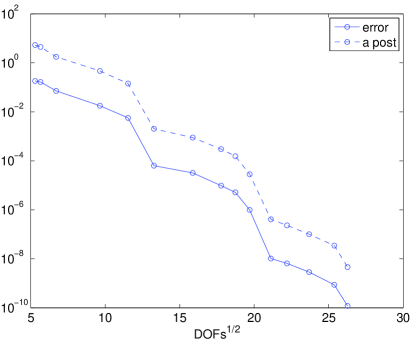
Figure 2. Errors and error estimates. Triangle problem.

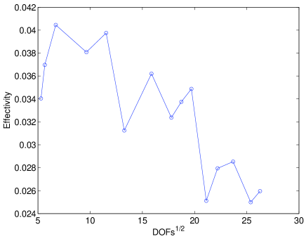
Figure 3. Effectivity index. Triangle problem.

In Figure 2 we plot the total relative error for the first four eigenvalues, together with the associated error estimate; and in Figure 3 we plot the effectivity quotient. It is clear that the convergence is exponential in this case, and that the effectivity undergoes a mild degradation as the problem size increases. This modest decrease in effectivity is in line with Remark 4.3, and it is also seen in our remaining experiments.

5.2. Dirichlet Laplacian on the Unit Triangle with on a Hole

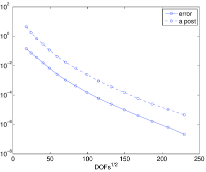
Figure 4. Errors and error estimates. Triangle with hole.

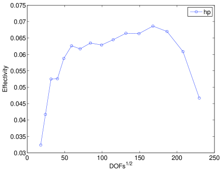
Figure 5. Effectivity index. Triangle with hole.

We now consider the problem where ${\mathcal{L}}=-\Delta$, $\Omega$ is the equilateral triangle having edge-length $2$ with an equilateral triangle having edge-length $1/2$ removed from its center (see Figure 1), and $\psi=0$ on $\partial\Omega$. For such a problem, it is expected that some of the eigenfunctions will have an $r^{3/5}$-type singularity at each of the three interior corners, where $r$ is the distance to the nearest corner. In this case, the exact eigenvalues are unknown, so we computed the following reference values of them on a very large problem: 40.4650426 for the first eigenvalue and 43.4868466 for the second and third, which form a double eigenvalue. These values are accurate at least up to 1e-6.

In Figure 4 we plot the relative error and error estimates together, for the first three eigenvalues, and in Figures 5 we plot the corresponding values of the effectivity quotient. We again see exponential convergence and a modest deterioration of effectivity.

5.3. Square Domain with Discontinuous Reaction Term

For this pair of problems we take $\Omega=(0,1)^{2}$, $\nabla\psi\cdot{\mathbf{n}}=0$ on $\partial\Omega$, and ${\mathcal{L}}\,\psi=-\Delta\psi+\kappa V_{MD}\cdot\psi$, where $V_{MD}$ is the characteristic function of the touching squares labelled ${\mathcal{M}}_{1}$ in Figure 6. We consider two values of the constant parameter, $\kappa=10,100$. It is straightforward to see that the corresponding bilinear form is an inner-product in this case (no zero eigenvalues), and that all eigenfunctions are at least in $H^{2}$.

Figure 6. A modification of the touching squares example of M. Dauge.

For $\kappa=10$, we have in Figure 7 the total relative error and error estimates for the first four eigenvalues; and the effectivity quotient is given in Figure 8. For these simulations we used the following reference values for the first four eigenvalues, which are 1e-8 accurate: 4.150242455, 10.706070962, 18.779725462, 25.150325247. The analogous plots for the first four eigenvalues in the case $\kappa=100$ are given in Figure 9 and Figure 10. For these simulations, we used the following reference values for the first four eigenvalues, which are 1e-8 accurate: 13.210576406, 13.990033964, 60.294151672, 64.840268299. In both cases we see apparent exponential convergence, and reasonable effectivity behavior. It seem clear from the error plots that for both values of $\kappa$ the convergence is exponential.

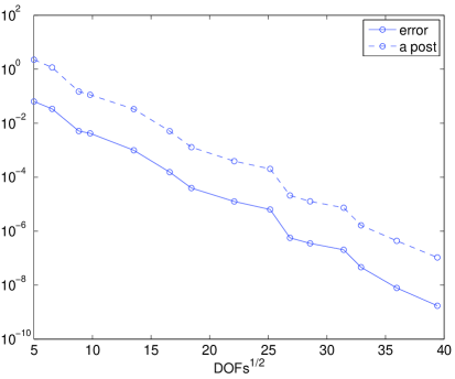
Figure 7. Errors and error estimates. Discontinuous reaction term, $\kappa=10$.

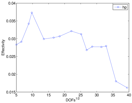
Figure 8. Effectivity index. Discontinuous reaction term, $\kappa=10$.

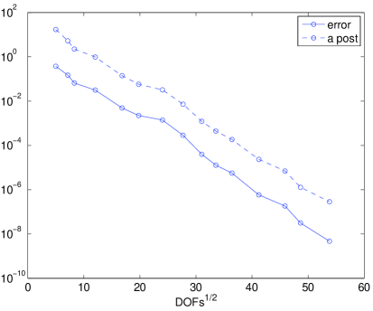
Figure 9. Errors and error estimates. Discontinuous reaction term, $\kappa=100$.

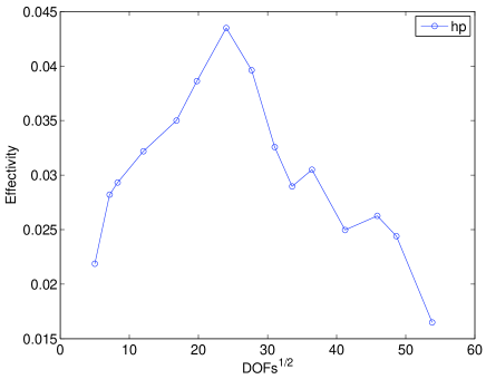
Figure 10. Effectivity index. Discontinuous reaction term, $\kappa=100$.

5.4. Square Domain with Discontinuous Diffusion Term

Using the domain $\Omega=(0,1)^{2}$, partitioned into regions ${\mathcal{M}}_{1}$ and ${\mathcal{M}}_{2}$ as in Figure 6, and homogeneous Dirichlet conditions $\psi=0$ on $\partial\Omega$, we consider the operator ${\mathcal{L}}=-\nabla\cdot(a\nabla)$, where $a=1$ in ${\mathcal{M}}_{2}$ and $a$ in ${\mathcal{M}}_{1}$ may vary. Such problems can have arbitrarily bad singularities at the cross-point of the domain depending on the relative sizes of $a$ in the two subdomains—see, for example, [13, 14] and [17, Example 5.3].

We have considered two values for $a$ in ${\mathcal{M}}_{1}$: 10 and 100. Since the exact eigenvalues are not available, we computed the following three reference values for the first three eigenvalues when $a=10$: 64.226529416, 75.028156269, 141.161506328; and the following three reference values for the first three eigenvalues when $a=100$: 77.800981966, 78.564198245, 193.916538067. All reference values are at least 1e-8 accurate. The relative error and effectivity plots for both cases are given in Figures 11-14, and again we see apparent exponential convergence.

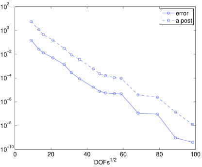
Figure 11. Errors and error estimates. Discontinuous diffusion term, $\kappa=10$.

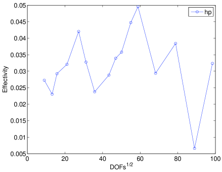
Figure 12. Effectivity index. Discontinuous diffusion term, $\kappa=10$.

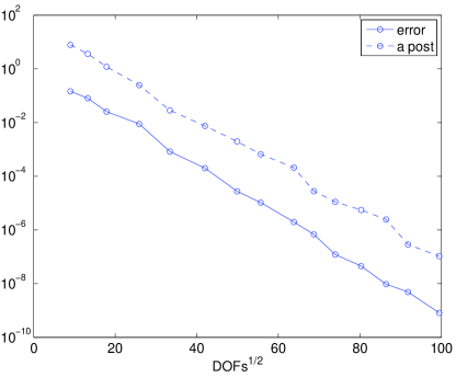
Figure 13. Errors and error estimates. Discontinuous diffusion term, $\kappa=100$.

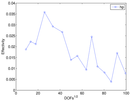
Figure 14. Effectivity index. Discontinuous diffusion term, $\kappa=100$.

5.5. Square Domain with a Slit

For this problem, ${\mathcal{L}}=-\Delta$ and $\Omega=(0,1)^{2}\setminus S$, where $S=\{(x,1/2):\,1/2<x<1\}$; this is pictured in Figure 1, with $S$ as the dashed segment. Homogeneous Neumann conditions are imposed on both “sides” of $S$ and homogeneous Dirichlet boundary conditions are imposed on the rest of the boundary of $\Omega$. For this example we used the following reference values for the first four eigenvalues with in brackets the corresponding accuracy: 20.739208802(8), 34.485320(5), 50.348022005(8), 67.581165196(8).

To give some indication of the nature of the eigenfunctions in the interior, we briefly consider a related problem where $\Omega$ is the unit disk with a slit along the positive $x$-axis, as pictured in Figure 1, with the same boundary conditions. In this case, the eigenvalues and eigenfunctions are known explicitly. For $k\geq 0$ and $m\geq 1$, let $z_{km}$ be the $m^{th}$ positive root of the first-kind Bessel function $J_{k/2}$. It is straightforward to verify that, up to renormalization of eigenfunctions, the eigenpairs can be indexed by

$$\lambda_{km}=z_{km}^{2}\quad,\quad\psi_{km}=J_{k/2}(z_{km}r)\sin(k\theta/2)\quad,\quad k,m\in\mathbb{N}~{}.$$

We see that $\psi_{km}\sim\sin(k\theta/2)\left(\frac{z_{km}r}{2}\right)^{1/2}$ as $r\to 0$, so singularities of types $r^{k/2}$ occur infinitely many times in the spectrum. The strongest of these singularities is of type $r^{1/2}$, and it occurs in the eigenfunction associated with the second eigenvalue, for example. The same asymptotic behavior of the eigenfunctions near the crack tip is expected for the square and circular domains, and in Figure 15 we show contour plots of the second eigenvalue in both cases. For the circular domain, the second eigenvalue and function can, in principle be obtained to arbitrary precision using a computer algebra system. Using Mathematica, we computed the second eigenvalue (the smallest positive root of $J_{1/2}$) to 20 digits, 9.869604401089358619, and generated the corresponding contour plot of the eigenfunction.

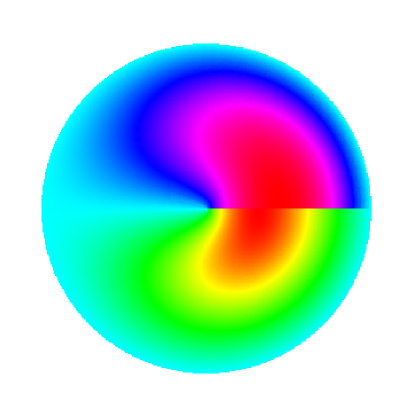
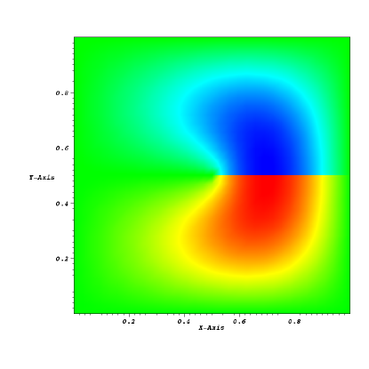
Figure 15. Second eigenfunction for the slit circle (top) and slit square.

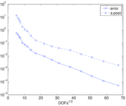
Figure 16. Errors and error estimates. Slit square. First four eigenvalues.

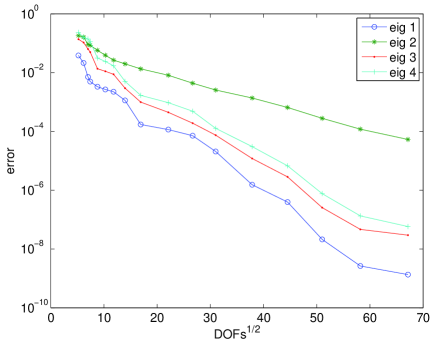
Figure 17. Errors from each eigenvlaue. Slit square.

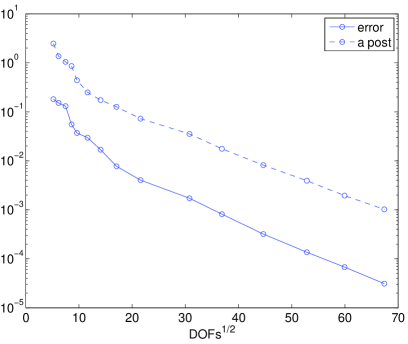
Figure 18. Errors and error estimates. Slit square. Second eigenvalue only.

In Figure 16 we plot the total relative errors and error estimates for the first four eigenvalues, and in Figure 17 the individual eigenvalue errors are shown. It is clear from the second of these figures that the second, which corresponds to the most singular eigenfunction, clearly has the worst convergence rate (as expected), and that this is what “spoils” the convergence of the cluster of the first four eigenvalues. This becomes even more apparent when Figure 18, which corresponds to the second eigenvalue alone, is compared with Figure 16—they are nearly identical.

References

- [1] H. Ammari, Y. Capdeboscq, H. Kang, and A. Kozhemyak. Mathematical models and reconstruction methods in magneto-acoustic imaging. European J. Appl. Math., 20(3):303–317, 2009.
- [2] H. Ammari, H. Kang, E. Kim, and H. Lee. Vibration testing for anomaly detection. Math. Methods Appl. Sci., 32(7):863–874, 2009.
- [3] H. Ammari, H. Kang, and H. Lee. Asymptotic analysis of high-contrast phononic crystals and a criterion for the band-gap opening. Arch. Ration. Mech. Anal., 193(3):679–714, 2009.
- [4] R. Bank, L. Grubišić, and J. S. Ovall. A framework for robust eigenvalue and eigenvector error estimation and ritz value convergence enhancement. submitted, MPI MSI Leipzig preprint 42/2010, 2010.
- [5] A. H. Barnett and T. Betcke. Stability and convergence of the method of fundamental solutions for Helmholtz problems on analytic domains. J. Comput. Phys., 227(14):7003–7026, 2008.
- [6] T. Betcke. A GSVD formulation of a domain decomposition method for planar eigenvalue problems. IMA J. Numer. Anal., 27(3):451–478, 2007.
- [7] T. Betcke and L. N. Trefethen. Reviving the method of particular solutions. SIAM Rev., 47(3):469–491 (electronic), 2005.
- [8] T. Eibner and J. Melenk. An adaptive strategy for hp-FEM based on testing for analyticity. Comp. Mech., 39:575–595, 2007.
- [9] S. C. Eisenstat. On the rate of convergence of the Bergman-Vekua method for the numerical solution of elliptic boundary value problems. SIAM J. Numer. Anal., 11:654–680, 1974.
- [10] S. Giani and I. G. Graham. Adaptive finite element methods for computing band gaps in photonic crystals. Numer. Math., (to appear), 2011.
- [11] S. Giani, L. Grubišić, and J. S. Ovall. Benchmark results for testing adaptive finite element eigenvalue procedures. Appl. Numer. Math., (to appear), 2011.
- [12] L. Grubišić and J. S. Ovall. On estimators for eigenvalue/eigenvector approximations. Math. Comp., 78:739–770, 2009.
- [13] R. B. Kellogg. On the Poisson equation with intersecting interfaces. Applicable Anal., 4:101–129, 1974/75. Collection of articles dedicated to Nikolai Ivanovich Muskhelishvili.
- [14] A. Knyazev and O. Widlund. Lavrentiev regularization + Ritz approximation = uniform finite element error estimates for differential equations with rough coefficients. Math. Comp., 72(241):17–40 (electronic), 2003.
- [15] B. J. McCartin. Eigenstructure of the equilateral triangle, part i: The dirichlet problem. SIAM Review, 45(2):pp. 267–287, 2003.
- [16] J. M. Melenk and B. I. Wohlmuth. On residual-based a posteriori error estimation in -FEM. Adv. Comput. Math., 15(1-4):311–331 (2002), 2001. A posteriori error estimation and adaptive computational methods.
- [17] P. Morin, R. H. Nochetto, and K. G. Siebert. Data oscillation and convergence of adaptive FEM. SIAM J. Numer. Anal., 38(2):466–488 (electronic), 2000.
- [18] B. Simon. Trace ideals and their applications, volume 35 of London Mathematical Society Lecture Note Series. Cambridge University Press, Cambridge, 1979.
- [19] R. Tankelevich, G. Fairweather, and A. Karageorghis. Three-dimensional image reconstruction using the PF/MFS technique. Eng. Anal. Bound. Elem., 33(12):1403–1410, 2009.