A Compiler for Variational Forms

Abstract

As a key step towards a complete automation of the finite element method, we present a new algorithm for automatic and efficient evaluation of multilinear variational forms. The algorithm has been implemented in the form of a compiler, the FEniCS Form Compiler FFC. We present benchmark results for a series of standard variational forms, including the incompressible Navier–Stokes equations and linear elasticity. The speedup compared to the standard quadrature-based approach is impressive; in some cases the speedup is as large as a factor 1000.

Robert C. Kirby, Department of Computer Science, University of Chicago, 1100 East 58th Street, Chicago, Illinois 60637, USA. Email: kirby@cs.uchicago.edu. This work was supported by the United States Department of Energy under grant DE-FG02-04ER25650.
Anders Logg, Toyota Technological Institute at Chicago, University Press Building, 1427 East 60th Street, Chicago, Illinois 60637, USA. Email: logg@tti-c.org.

1 Introduction

The finite element method provides a general mathematical framework for the solution of differential equations and can be viewed as a machine that automates the discretization of differential equations; given the variational formulation of a differential equation, the finite element method generates a discrete system of equations for the approximate solution.

This generality of the finite element method is seldom reflected in codes, which are often very specialized and can only solve one particular differential equation or a small set of differential equations.

There are two major reasons that the finite element method has yet to be fully automated; the first is the complexity of the task itself, and the second is that specialized codes often outperform general codes. We address both these concerns in this paper.

A basic task of the finite element method is the computation of the element stiffness matrix from a bilinear form on a local element. In many applications, computation of element stiffness matrices accounts for a substantial part of the total run-time of the code. [Kirby et al. (2005), SISC] This routine is a small amount of code, but it can be tedious to get it both correct and efficient. While the standard quadrature-based approach to computing the element stiffness matrix works on very general variational forms, it is well-known that precomputing certain quantities in multilinear forms can improve the efficiency of building finite element matrices.

The methods discussed in this paper for efficient computation of element stiffness matrices are based on ideas previously presented in [Kirby et al. (2005), SISC] and [Kirby et al. (2005), BIT], where the basic idea is to represent the element stiffness matrix as a tensor product. A similar approach has been implemented earlier in the finite element library DOLFIN [Hoffman et al. (2005), Hoffman and Logg (2002)], but only for linear elements. The current paper generalizes and formalizes these ideas and presents an algorithm for generation of the tensor representation of element stiffness matrices and for evaluation of the tensor product. This algorithm has been implemented in the form of the compiler FFC for variational forms; the compiler takes as input a variational form in mathematical notation and automatically generates efficient code (C or C++) for computation of element stiffness matrices and their insertion into a global sparse matrix. This includes the generation of code both for the computation of element stiffness matrices and local-to-global mappings of degrees of freedom.

1.1 FEniCS and the Automation of CMM

FFC, the FEniCS Form Compiler, is a central component of FEniCS [Hoffman et al. (2005)], a project for the Automation of Computational Mathematical Modeling (ACMM). The central task of ACMM, as formulated in [Logg (2004)], is to create a machine that takes as input a model $R(u)=A(u)-f$, a tolerance $\mathrm{TOL}>0$ and a norm $\|\cdot\|$ (or some other measure of quality), and produces as output an approximate solution $U\approx u$ that satisfies the accuracy requirement $\|U-u\|<\mathrm{TOL}$ using a minimal amount of work (see Figure 1). This includes an aspect of reliability (the produced solution should satisfy the accuracy requirement) and an aspect of efficiency (the solution should be obtained with minimal work).

\psfrag{in1}{$R(u)=0$}\psfrag{in2}{$\mathrm{TOL}>0$}\psfrag{ut}{$U\approx u$}\includegraphics[width=284.52756pt]{eps/automation-2-1.eps}

Figure 1: The Automation of Computational Mathematical Modeling.

In many applications, several competing models are under consideration, and one would like to computationally compare them. Developing separate, special purpose codes for each model is prohibitive. Hence, a key step of ACMM is the automation of discretization, i.e., the automatic translation of a differential equation into a discrete system of equations, and as noted above this key step is automated by the finite element method. The FEniCS Form Compiler FFC may then be viewed as an important step towards the automation of the finite element method, and thus as an important step towards the Automation of CMM.

FEniCS software is free software. In particular, FFC is licensed under the GNU General Public License [Free Software Foundation (1991)]. All FEniCS software is available for download on the FEniCS web site [Hoffman et al. (2005)]. In Section 5.6, we return to a discussion of the different components of FEniCS and their relation to FFC.

1.2 Current finite element software

Several emerging projects seek to automate important aspects of the finite element method. By developing libraries in existing languages or new domain-specific languages, software tools may be built that allow programmers to define variational forms and other parts of a finite element method with succinct, mathematical syntax. Existing C++ libraries for finite elements include DOLFIN [Hoffman et al. (2005), Hoffman and Logg (2002)], Sundance [Long (2003)], deal.II [Bangerth et al. (2005)], Diffpack [Langtangen (1999)] and FEMSTER [Castillo et al. (2004), Castillo et al. (2005)]. Projects developing domain-specific languages for finite element computation include FreeFEM [Pironneau et al. (2005)] and GetDP [Dular and Geuzaine (2005)]. A precursor to the FEniCS project, Analysa [Bagheri and Scott (2003)], was a Scheme-like language for finite element methods. Earlier work on object-oriented frameworks for finite element computation include [Mackie (1992)] and [Masters et al. (1997)].

While these tools are effective at exploiting modern software engineering to produce workable systems, we believe that additional mathematical insight will lead to even more powerful codes with more general approximating spaces and more powerful algorithms. The FEniCS project is more ambitious than to just collect and implement existing ideas.

1.3 Design goals

The primary design goal for FFC is to accept as input “any” multilinear variational form and “any” finite element, and to generate code that will run with close to optimal performance.

We will make precise below in Section 3.2 which forms and which elements the compiler can currently handle (general multilinear variational forms with coefficients over affine simplices).

A secondary goal for FFC is to create a new standard in form evaluation; hopefully FFC can become a standard tool for practitioners solving partial differential equations using the finite element method. In addition to generating very efficient code for evaluation of the element stiffness matrix, FFC thus takes away the burden of having to implement the code from the developer. Furthermore, if the code for the element stiffness matrix is generated by a compiler that is trusted and has gone through rigorous testing, it is easier to achieve correctness of a simulation code.

The primary output target of FFC is the C++ library DOLFIN. By default, FFC accepts as input a variational form and generates code for the evaluation of the variational form in DOLFIN, as illustrated in Figure 2. Although FFC works closely with other FEniCS components, such as DOLFIN, it has an abstraction layer that allows it to be hooked up to multiple backends. One example of this is the newly added ASE (ANL SIDL Environment, [Balay et al. (2005a)]) format added to FFC, allowing forms to be compiled for the next generation of PETSc [Balay et al. (2005b)].

\psfrag{FFC}{\ \large{{FFC}}}\psfrag{form}{\hskip 15.6491pt$a(v,u)=\int_{\Omega}\nabla v(x)\cdot\nabla u(x)\,\mathrm{d}x$}\includegraphics[width=284.52756pt]{eps/ffc.eps}

Figure 2: The form compiler FFC takes as input a variational form and generates code for evaluation of the form.

1.4 The compiler approach

It is widely accepted in developing software for scientific computing that there is a trade-off between generality and efficiency; a software component that is general in nature, i.e., it accepts a wide range of inputs, is often less efficient than another software component that performs the same job on a more limited set of inputs. As a result, most codes used by practitioners for the solution of differential equations are very specific.

However, by using a compiler approach, it is possible to combine generality and efficiency without loss of generality and without loss of efficiency. This is possible since our compiler works on a very small family of inputs (multilinear variational forms) with sharply defined mathematical properties. Our domain-specific knowledge allows us to generate much better code than if we used general-purpose compiler techniques.

1.5 Outline of this paper

Before presenting the main algorithm, we give a short background on the implementation of the finite element method and the evaluation of variational forms in Section 2. The main algorithm is then outlined in Section 3. In Section 4, we compare the complexity of form evaluation for the algorithm used by FFC with the standard quadrature-based approach. We then discuss the implementation of the form compiler in some detail in Section 5.

In Section 6, we compare the CPU time for evaluating a series of standard variational forms using code automatically generated by FFC and hand-coded quadrature-based implementations. The speedup is in all cases significant, in the case of cubic Lagrange elements on tetrahedra a factor 100 (Figure 3).

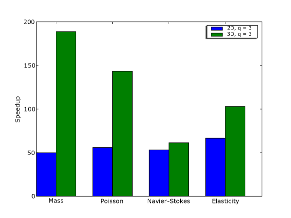
Figure 3: Speedup for a series of standard variational forms (here compiled for cubic Lagrange elements on triangles and tetrahedra, respectively).

Finally, in Section 7, we summarize the current features and shortcomings of FFC and give directions for future development and research.

2 Background

In this section, we present a quick background on the finite element method. The material is standard [Ciarlet (1976), Hughes (1987), Brenner and Scott (1994), Eriksson et al. (1996)], but is included here to give a context for the presentation of the form compiler and to summarize the notation used throughout the remainder of this paper.

For simplicity, we consider here only linear partial differential equations and note that these play an important role in the discretization of nonlinear partial differential equations (in Newton or fixed-point iterations).

2.1 Variational forms

We work with the standard variational formulation of a partial differential equation: Find $u\in V$ such that

$$a(v,u)=L(v)\quad\forall v\in\hat{V},$$ (1)

with $a:\hat{V}\times V\rightarrow\mathbb{R}$ a bilinear form, $L:\hat{V}\rightarrow\mathbb{R}$ a linear form, and $(\hat{V},V)$ a pair of suitable function spaces. For the standard example, Poisson’s equation $-\Delta u(x)=f(x)$ with homogeneous Dirichlet conditions on a domain $\Omega$, the bilinear form $a$ is given by $a(v,u)=\int_{\Omega}\nabla v(x)\cdot\nabla u(x)\,\mathrm{d}x$, the linear form $L$ is given by $L(v)=\int_{\Omega}v(x)f(x)\,\mathrm{d}x$, and $\hat{V}=V=H^{1}_{0}(\Omega)$.

The finite element method discretizes (1) by replacing $(\hat{V},V)$ with a pair of (piecewise polynomial) discrete function spaces. With $\{\hat{\phi}_{i}\}_{i=1}^{M}$ a basis for the test space $\hat{V}$ and $\{\phi_{i}\}_{i=1}^{M}$ a basis for the trial space $V$, we can expand the approximate solution $U$ of (1) in the basis functions of $V$, $U=\sum_{j=1}^{M}\xi_{j}\phi_{j}$, and obtain a linear system $A\xi=b$ for the degrees of freedom $\{\xi_{j}\}_{j=1}^{M}$ of the approximate solution $U$. The entries of the matrix $A$ and the vector $b$ defining the linear system are given by

$$\begin{split}A_{ij}&=a(\hat{\phi}_{i},\phi_{j}),\quad i,j=1,\ldots,M,\\ b_{i}&=L(\hat{\phi}_{i}),\quad i=1,\ldots,M.\end{split}$$ (2)

2.2 Assembly

The standard algorithm for computing the matrix $A$ (or the vector $b$) is assembly; the matrix is computed by iteration over the elements $K$ of a triangulation $\mathcal{T}$ of $\Omega$, and the contribution from each local element is added to the global matrix $A$.

To see this, we note that if the bilinear form $a$ is expressed as an integral over the domain $\Omega$, we can write the bilinear form as a sum of element bilinear forms, $a(v,u)=\sum_{K\in\mathcal{T}}a_{K}(v,u)$, and thus

$$A_{ij}=\sum_{K\in\mathcal{T}}a_{K}(\hat{\phi}_{i},\phi_{j}),\quad i,j=1,\ldots,M.$$ (3)

In the case of Poisson’s equation, the element bilinear form $a_{K}$ is defined by $a_{K}(v,u)=\int_{K}\nabla v(x)\cdot\nabla u(x)\,\mathrm{d}x$.

Let now $\{\hat{\phi}_{i}^{K}\}_{i=1}^{n}$ be the restriction to $K$ of the subset of $\{\hat{\phi}_{i}\}_{i=1}^{M}$ supported on $K$ and $\{\phi_{i}^{K}\}_{i=1}^{n}$ the corresponding local basis for $V$. Furthermore, let $\hat{\iota}(\cdot,\cdot)$ be a mapping from the local numbering scheme to the global numbering scheme (local-to-global mapping) for the basis functions of $\hat{V}$, so that $\hat{\phi}_{i}^{K}$ is the restriction to $K$ of $\phi_{\hat{\iota}(K,i)}$, and let $\iota(K,\cdot)$ be the corresponding mapping for $V$. We may now express an algorithm for the computation of the matrix $A$ (Algorithm 1).

$A=0$

for $K\in\mathcal{T}$

for $i=1,\ldots,n$

for $j=1,\ldots,n$

$A_{\hat{\iota}(K,i)\iota(K,j)}=A_{\hat{\iota}(K,i)\iota(K,j)}+a_{K}(\hat{\phi}^{K}_{i},\phi_{j}^{K})$

end for

end for

end for

Algorithm 1 $A$ = Assemble($a$, $\mathcal{T}$, $\hat{V}$, $V$)

Alternatively, one may define the element matrix $A^{K}$ by

$$A^{K}_{ij}=a_{K}(\hat{\phi}^{K}_{i},\phi_{j}^{K})\quad i,j=1,\ldots,n,$$ (4)

and separate the computation on each element $K$ into two steps: computation of the element matrix $A^{K}$ and insertion of $A^{K}$ into $A$ (Algorithm 2).

$A=0$

for $K\in\mathcal{T}$

Compute $A^{K}$ according to (4)

Add $A^{K}$ to $A$ using the local-to-global mappings $(\hat{\iota}(K,\cdot),\iota(K,\cdot))$

end for

Algorithm 2 $A$ = Assemble($a$, $\mathcal{T}$, $\hat{V}$, $V$)

Separating the two concerns of computing the element matrix $A^{K}$ and adding it to the global matrix $A$ as in Algorithm 2 has the advantage that one may use an optimized library routine for adding the element matrix $A^{K}$ to the global matrix $A$. Sparse matrix libraries such as PETSc [Balay et al. (2005b), Balay et al. (2004), Balay et al. (1997)] often provide optimized routines for this type of operation. Note that the cost of adding $A^{K}$ to $A$ may be substantial even with an efficient implementation of the sparse data structure for $A$ [Kirby et al. (2005), SISC].

As we shall see below, we may also take advantage of the separation of concerns of Algorithm 2 to optimize the computation of the element matrix $A^{K}$. This step is automated by the form compiler FFC. Given a bilinear (or multilinear) form $a$, FFC automatically generates code for run-time computation of the element matrix $A^{K}$.

3 Evaluation of multilinear forms

In this section, we present the algorithm used by FFC to automatically generate efficient code for run-time computation of the element matrix $A^{K}$.

3.1 Multilinear forms

Let $\{V_{i}\}_{i=1}^{r}$ be a given set of discrete function spaces defined on a triangulation $\mathcal{T}$ of $\Omega\subset\mathbb{R}^{d}$. We consider a general multilinear form $a$ defined on the product space $V_{1}\times V_{2}\times\cdots\times V_{r}$:

$$a:V_{1}\times V_{2}\times\cdots\times V_{r}\rightarrow\mathbb{R}.$$ (5)

Typically, $r=1$ (linear form) or $r=2$ (bilinear form), but the form compiler FFC can handle multilinear forms of arbitrary arity $r$. Forms of higher arity appear frequently in applications and include variable coefficient diffusion and advection of momentum in the incompressible Navier–Stokes equations.

Let now $\{\phi_{i}^{1}\}_{i=1}^{M_{1}},\{\phi_{i}^{2}\}_{i=1}^{M_{2}},\ldots,\{\phi_{i}^{r}\}_{i=1}^{M_{r}}$ be bases of $V_{1},V_{2},\ldots,V_{r}$ and let $i=(i_{1},i_{2},\ldots,i_{r})$ be a multiindex. The multilinear form $a$ then defines a rank $r$ tensor given by

$$A_{i}=a(\phi_{i_{1}}^{1},\phi_{i_{2}}^{2},\ldots,\phi_{i_{r}}^{r}).$$ (6)

In the case of a bilinear form, the tensor $A$ is a matrix (the stiffness matrix), and in the case of a linear form, the tensor $A$ is a vector (the load vector).

As discussed in the previous section, to compute the tensor $A$ by assembly, we need to compute the element tensor $A^{K}$ on each element $K$ of the triangulation $\mathcal{T}$ of $\Omega$. Let $\{\phi^{K,1}_{i}\}_{i=1}^{n_{1}}$ be the restriction to $K$ of the subset of $\{\phi_{i}^{1}\}_{i=1}^{M_{1}}$ supported on $K$ and define the local bases on $K$ for $V_{2},\ldots,V_{r}$ similarly. The rank $r$ element tensor $A^{K}$ is then defined by

$$A^{K}_{i}=a_{K}(\phi_{i_{1}}^{K,1},\phi_{i_{2}}^{K,2},\ldots,\phi_{i_{r}}^{K,r}).$$ (7)

3.2 Evaluation by tensor representation

The element tensor $A^{K}$ can be efficiently computed by representing $A^{K}$ as a special tensor product. Under some mild assumptions which we shall make precise below, the element tensor $A^{K}$ can be represented as the tensor product of a reference tensor $A^{0}$ and a geometry tensor $G_{K}$:

$$A^{K}_{i}=A^{0}_{i\alpha}G_{K}^{\alpha},$$ (8)

or more generally a sum $A^{K}_{i}=A^{0,k}_{i\alpha}G_{K,k}^{\alpha}$ of such tensor products, where $i$ and $\alpha$ are multiindices and we use the convention that repetition of an index means summation over that index. The rank of the reference tensor is the sum of the rank $r=|i|$ of the element tensor and the rank $|\alpha|$ of the geometry tensor $G_{K}$. As we shall see, the rank of the geometry tensor depends on the specific form and is typically a function of the Jacobian of the mapping from the reference element and any variable coefficients appearing in the form.

Our goal is to develop an algorithm that converts an abstract representation of a multilinear form into (i) the values of the reference tensor $A^{0}$ and (ii) an expression for evaluating the geometry tensor $G_{K}$ for any given element $K$. Note that $A^{0}$ is fixed and independent of the element $K$ and may thus be precomputed. Only $G_{K}$ has to be computed on each element. As we shall see below in Section 4, for a wide range of multilinear forms, this allows for computation of the element tensor $A^{K}$ using far fewer floating-point operations than if the element tensor $A^{K}$ were computed by quadrature on each element $K$.

To see how to obtain the tensor representation (8), we fix a small set of operations, allowing only multilinear forms that can be expressed through these operations, and observe how the tensor representation (8) transforms under these operations. As we shall see below, this covers a wide range of multilinear forms (but not all). We first develop the tensor representation in abstract form and then present a number of test cases that exemplify the general notation in Section 3.3.

As basic elements, we take the local basis functions $\{\phi_{\gamma}\}_{\gamma}=\cup_{i}\{\phi^{K,i}_{j}\}_{j=1}^{n_{i}}$ for a set of finite element spaces $V_{i}$, $i=1,2,\ldots$, including the finite element spaces $V_{1},V_{2},\ldots,V_{r}$ on which the multilinear form is defined. Allowing addition $\phi_{1}+\phi_{2}$ and multiplication with scalars $\alpha\phi$, we obtain a vector space $\mathcal{A}$ of linear combinations of basis functions. Since $\phi_{1}-\phi_{2}=\phi_{1}+(-1)\phi_{2}$ and $\phi/\alpha=(1/\alpha)\phi$, we can easily equip the vector space with subtraction and division by scalars.

We next equip our vector space with multiplication between elements of the vector space. We thus obtain an algebra $\mathcal{A}$ of linear combinations of products of basis functions. Finally, we extend $\mathcal{A}$ by adding differentiation $\partial/\partial x_{i}$ with respect to a coordinate direction $x_{i}$, $i=1,\ldots,d$, on $K$, to obtain

$$\mathcal{A}=\{v:v=\sum c_{(\cdot)}\prod\frac{\partial^{|(\cdot)|}\phi_{(\cdot)}}{\partial x_{(\cdot)}}\},$$ (9)

where $(\cdot)$ represents some multiindex.

To summarize, $\mathcal{A}$ is the algebra of linear combinations of products of basis functions or derivatives of basis functions that is generated from the set of basis functions through addition ($+$), subtraction ($-$), multiplication $(\cdot)$, including multiplication with scalars, division by scalars $(/)$, and differentiation $\partial/\partial x_{i}$. Note that if the basis functions are vector-valued (or tensor-valued), the algebra is generated from the set of scalar components of the basis functions.

We may now state precisely the multilinear forms that the form compiler FFC can handle, namely those multilinear forms that can be expressed as integrals over $K$ (or the boundary of $K$) of elements of the algebra $\mathcal{A}$. Note that not all integrals over $K$ of elements of $\mathcal{A}$ are multilinear forms; in particular, each product needs to be linear in each argument of the form.

The tensor representation (8) now follows by a standard change of variables using an affine mapping $F_{K}:K_{0}\rightarrow K$ from a reference element $K_{0}$ to the current element $K$ (see Figure 4). With $\{\Phi_{\gamma}\}_{\gamma}$ the basis functions on the reference element corresponding to $\{\phi_{\gamma}\}_{\gamma}$, defined by $\Phi_{\gamma}=\phi_{\gamma}\circ F_{K}$, we obtain the following representation of the element tensor $A^{K}$ corresponding to $v_{i}=\left(\sum c_{(\cdot)}\prod\frac{\partial^{|(\cdot)|}\phi_{(\cdot)}}{\partial x_{(\cdot)}}\right)_{i}$:

$$\begin{split}A^{K}_{i}&=a_{K}(\phi_{i_{1}}^{K,1},\phi_{i_{2}}^{K,2},\ldots,\phi_{i_{r}}^{K,r})=\int_{K}v_{i}\,\mathrm{d}x\\ &=\left(\int_{K}\sum c_{(\cdot)}\prod\frac{\partial^{|(\cdot)|}\phi_{(\cdot)}}{\partial x_{(\cdot)}}\,\mathrm{d}x\right)_{i}=\sum\left(c_{(\cdot)}\int_{K}\prod\frac{\partial^{|(\cdot)|}\phi_{(\cdot)}}{\partial x_{(\cdot)}}\,\mathrm{d}x\right)_{i}\\ &=\sum\left(c_{(\cdot)}\det F_{K}^{\prime}\prod\frac{\partial X_{(\cdot)}}{\partial x_{(\cdot)}}\right)_{\alpha}\left(\int_{K_{0}}\prod\frac{\partial^{|(\cdot)|}\Phi_{(\cdot)}}{\partial X_{(\cdot)}}\,\mathrm{d}X\right)_{i\alpha}\\ &=A^{0,k}_{i\alpha}G_{K,k}^{\alpha},\end{split}$$ (10)

where

$$A^{0,k}_{i\alpha} =\left(\int_{K_{0}}\prod\frac{\partial^{|(\cdot)|}\Phi_{(\cdot)}}{\partial X_{(\cdot)}}\,\mathrm{d}X\right)_{i\alpha},$$ (11)

$$G_{K,k}^{\alpha} =\left(c_{(\cdot)}\det F_{K}^{\prime}\prod\frac{\partial X_{(\cdot)}}{\partial x_{(\cdot)}}\right)_{\alpha}.$$ (12)

We have here used the fact that the mapping is affine to pull the determinant and transforms of derivatives outside of the integral. For a discussion of non-affine mappings, including the Piola transform and isoparametric mapping, see Section 3.4 below.

Note that the expression for the geometry tensor $G_{K,k}$ implicitly contains a summation if an index is repeated twice. Also note that the geometry tensor contains any variable coefficients appearing in the form.

As we shall see below in Section 5, the representation of a multilinear form as an integral over $K$ of an element of $\mathcal{A}$ is automatically available to the form compiler FFC, since a multilinear form must be specified using the basic operations that generate $\mathcal{A}$.

\psfrag{p0}{$X^{1}=(0,0)$}\psfrag{p1}{$X^{2}=(1,0)$}\psfrag{p2}{$X^{3}=(0,1)$}\psfrag{xi}{$X$}\psfrag{x}{$x=F_{K}(X)$}\psfrag{F=}{}\psfrag{F}{$F_{K}$}\psfrag{x0}{$x^{1}$}\psfrag{x1}{$x^{2}$}\psfrag{x2}{$x^{3}$}\psfrag{K0}{$K_{0}$}\psfrag{K}{$K$}\includegraphics[width=312.9803pt]{eps/affinemap.eps}

Figure 4: The affine mapping $F_{K}$ from the reference element $K_{0}$ to the current element $K$.

3.3 Test cases

To make these ideas concrete, we write down the explicit tensor representation (8) of the element tensor $A^{K}$ for a series of standard forms. We return to these test cases below in Section 6 when we present benchmark results for each test case.

Test case 1: the mass matrix

As a first simple example, we consider the computation of the mass matrix $M$ with $M_{i_{1}i_{2}}=a(\phi^{1}_{i_{1}},\phi^{2}_{i_{2}})$ and the bilinear form $a$ given by

$$a(v,u)=\int_{\Omega}v(x)u(x)\,\mathrm{d}x.$$ (13)

By a change of variables given by the affine mapping $F_{K}:K_{0}\rightarrow K$, we obtain

$$A^{K}_{i}=\int_{K}\phi^{K,1}_{i_{1}}(x)\phi^{K,2}_{i_{2}}(x)\,\mathrm{d}x=\det F_{K}^{\prime}\int_{K_{0}}\Phi^{1}_{i_{1}}(X)\Phi^{2}_{i_{2}}(X)\,\mathrm{d}X=A^{0}_{i}G_{K},$$ (14)

where $A^{0}_{i}=\int_{K_{0}}\Phi_{i_{1}}^{1}(X)\Phi_{i_{2}}^{2}(X)\,\mathrm{d}X$ and $G_{K}=\det F_{K}^{\prime}$. In this case, the reference tensor $A^{0}$ is a rank two tensor (a matrix) and the geometry tensor $G_{K}$ is a rank zero tensor (a scalar). By precomputing the reference tensor $A^{0}$, we may thus compute the element tensor $A^{K}$ on each element $K$ by just multiplying the precomputed reference tensor with the determinant of (the derivative of) the affine mapping $F_{K}$.

Test case 2: Poisson’s equation

As a second example, consider the bilinear form for Poisson’s equation,

$$a(v,u)=\int_{\Omega}\nabla v(x)\cdot\nabla u(x)\,\mathrm{d}x.$$ (15)

By a change of variables as above, we obtain the following representation of the element tensor $A^{K}$:

$$\begin{split}A^{K}_{i}&=\int_{K}\nabla\phi^{K,1}_{i_{1}}(x)\cdot\nabla\phi^{K,2}_{i_{2}}(x)\,\mathrm{d}x\\ &=\det F_{K}^{\prime}\frac{\partial X_{\alpha_{1}}}{\partial x_{\beta}}\frac{\partial X_{\alpha_{2}}}{\partial x_{\beta}}\int_{K_{0}}\frac{\partial\Phi^{1}_{i_{1}}(X)}{\partial X_{\alpha_{1}}}\frac{\partial\Phi^{2}_{i_{2}}(X)}{\partial X_{\alpha_{2}}}\,\mathrm{d}X=A^{0}_{i\alpha}G_{K}^{\alpha},\end{split}$$ (16)

where $A^{0}_{i\alpha}=\int_{K_{0}}\frac{\partial\Phi^{1}_{i_{1}}(X)}{\partial X_{\alpha_{1}}}\frac{\partial\Phi^{2}_{i_{2}}(X)}{\partial X_{\alpha_{2}}}\,\mathrm{d}X$ and $G_{K}^{\alpha}=\det F_{K}^{\prime}\frac{\partial X_{\alpha_{1}}}{\partial x_{\beta}}\frac{\partial X_{\alpha_{2}}}{\partial x_{\beta}}$. We see that the reference tensor $A^{0}$ is here a rank four tensor and the geometry tensor $G_{K}$ is a rank two tensor (one index for each derivative appearing in the form).

Test case 3: Navier–Stokes

Consider now the nonlinear term $u\cdot\nabla u$ of the incompressible Navier–Stokes equations,

$$\begin{split}\dot{u}+u\cdot\nabla u-\nu\Delta u+\nabla p&=f,\\ \nabla\cdot u&=0.\end{split}$$ (17)

To solve the Navier–Stokes equations by fixed-point iteration (see for example [Eriksson et al. (2003)]), we write the nonlinear term in the form $u\cdot\nabla u=w\cdot\nabla u$ with $w=u$ and consider $w$ as fixed. We then obtain the following bilinear form:

$$a(v,u)=a_{w}(v,u)=\int_{\Omega}v(x)\cdot(w(x)\cdot\nabla)u(x)\,\mathrm{d}x.$$ (18)

Note that we may alternatively think of this as a trilinear form, $a=a(v,u,w)$.

Let now $\{w^{K}_{\alpha}\}_{\alpha}$ be the expansion coefficients for $w$ in a finite element basis on the current element $K$, and let $v{\scriptstyle[i]}$ denote component $i$ of a vector-valued function $v$. Furthermore, assume that $u$ and $w$ are discretized using the same discrete space $V=V_{2}$. We then obtain the following representation of the element tensor $A^{K}$:

$$\begin{split}A^{K}_{i}&=\int_{K}\phi^{K,1}_{i_{1}}(x)\cdot(w(x)\cdot\nabla)\phi^{K,2}_{i_{2}}(x)\,\mathrm{d}x\\ &=\det F_{K}^{\prime}\frac{\partial X_{\alpha_{3}}}{\partial x_{\alpha_{1}}}w^{K}_{\alpha_{2}}\int_{K_{0}}\Phi^{1}_{i_{1}}{\scriptstyle[\beta]}(X)\Phi^{2}_{\alpha_{2}}{\scriptstyle[\alpha_{1}]}(X)\frac{\partial\Phi^{2}_{i_{2}}{\scriptstyle[\beta]}(X)}{\partial X_{\alpha_{3}}}\,\mathrm{d}X=A^{0}_{i\alpha}G_{K}^{\alpha},\end{split}$$ (19)

where $A^{0}_{i\alpha}=\int_{K_{0}}\Phi^{1}_{i_{1}}{\scriptstyle[\beta]}(X)\Phi^{2}_{\alpha_{2}}{\scriptstyle[\alpha_{1}]}(X)\frac{\partial\Phi^{2}_{i_{2}}{\scriptstyle[\beta]}(X)}{\partial X_{\alpha_{3}}}\,\mathrm{d}X$ and $G_{K}^{\alpha}=\det F_{K}^{\prime}\frac{\partial X_{\alpha_{3}}}{\partial x_{\alpha_{1}}}w^{K}_{\alpha_{2}}$. In this case, the reference tensor $A^{0}$ is a rank five tensor and the geometry tensor $G_{K}$ is a rank three tensor (one index for the derivative, one for the function $w$, and one for the scalar product).

Test case 4: linear elasticity

Finally, consider the strain-strain term of linear elasticity,

$$\begin{split}a(v,u)&=\int_{\Omega}\frac{1}{4}(\nabla v+(\nabla v)^{\top}):(\nabla u+(\nabla u)^{\top})\,\mathrm{d}x\\ &=\int_{\Omega}\frac{1}{4}\frac{\partial v_{i}}{\partial x_{j}}\frac{\partial u_{i}}{\partial x_{j}}\,\mathrm{d}x+\frac{1}{4}\frac{\partial v_{i}}{\partial x_{j}}\frac{\partial u_{j}}{\partial x_{i}}\,\mathrm{d}x+\frac{1}{4}\frac{\partial v_{j}}{\partial x_{i}}\frac{\partial u_{i}}{\partial x_{j}}\,\mathrm{d}x+\frac{1}{4}\frac{\partial v_{j}}{\partial x_{i}}\frac{\partial u_{j}}{\partial x_{i}}\,\mathrm{d}x.\end{split}$$ (20)

Considering here only the first term, a change of variables leads to the following representation of the element tensor $A^{K,1}$:

$$\begin{split}A^{K,1}_{i}&=\int_{K}\frac{1}{4}\frac{\partial\phi^{K,1}_{i_{1}}{\scriptstyle[\beta_{1}]}(x)}{\partial x_{\beta_{2}}}\frac{\partial\phi^{K,2}_{i_{2}}{\scriptstyle[\beta_{1}]}(x)}{\partial x_{\beta_{2}}}\,\mathrm{d}x\\ &=\frac{1}{4}\det F_{K}^{\prime}\frac{\partial X_{\alpha_{1}}}{\partial x_{\beta_{2}}}\frac{\partial X_{\alpha_{2}}}{\partial x_{\beta_{2}}}\int_{K_{0}}\frac{\partial\Phi^{1}_{i_{1}}{\scriptstyle[\beta_{1}]}(X)}{\partial X_{\alpha_{1}}}\frac{\partial\Phi^{2}_{i_{2}}{\scriptstyle[\beta_{1}]}(X)}{\partial X_{\alpha_{2}}}\,\mathrm{d}X=A^{0,1}_{i\alpha}G_{K,1}^{\alpha},\end{split}$$ (21)

where $A^{0,1}_{i\alpha}=\int_{K_{0}}\frac{\partial\Phi^{1}_{i_{1}}{\scriptstyle[\beta_{1}]}(X)}{\partial X_{\alpha_{1}}}\frac{\partial\Phi^{2}_{i_{2}}{\scriptstyle[\beta_{1}]}(X)}{\partial X_{\alpha_{2}}}\,\mathrm{d}X$ and $G_{K,1}^{\alpha}=\frac{1}{4}\det F_{K}^{\prime}\frac{\partial X_{\alpha_{1}}}{\partial x_{\beta_{2}}}\frac{\partial X_{\alpha_{2}}}{\partial x_{\beta_{2}}}$. Here, the reference tensor $A^{0,1}$ is a rank four tensor and the geometry tensor $G_{K,1}$ is a rank two tensor (one index for each derivative).

3.4 Extensions

The current implementation of FFC supports only affinely mapped Lagrange elements and linear problems, but it is interesting to consider the generalization of our approach to other kinds of function spaces such as Raviart-Thomas [Raviart and Thomas (1977)] elements for $H(\mathrm{div})$ and curvilinear mappings such as arise with isoparametric elements, as well as how nonlinear problems may also be automated.

3.4.1 $H(\mathrm{div})$ and $H(\mathrm{curl})$ conforming elements

Implementing of $H(\mathrm{div})$ or $H(\mathrm{curl})$ elements requires two kinds of generalizations to FFC. First of all, the basis functions are mapped from the reference element by the Piola transform [Brezzi and Fortin (1991)] rather than the standard change of coordinates. With $F_{K}:K_{0}\rightarrow K$ the standard affine mapping for an element $K$, $F^{\prime}_{K}$ the Fréchet derivative of the mapping and $\det{F^{\prime}_{K}}$ its determinant, the Piola mapping is defined by $\mathcal{F}_{K}(\Psi)=\frac{1}{\det{F^{\prime}_{K}}}F^{\prime}_{K}(\Psi\circ\left(F_{K}\right)^{-1})$. Since our tools already track Jacobians and determinants for differentiating through affine mappings, it should be straightforward to support the Piola mapping. Second, defining the mapping between local and global degrees of freedom becomes more complicated, as we must keep track of directions of vector components as done in FEMSTER [Castillo et al. (2004), Castillo et al. (2005)].

As an example of using the Piola transform, we consider the Raviart-Thomas elements with the standard (vector-valued) nodal basis $\{\Psi_{i}\}_{i=1}^{d}$ on the reference element. We compute the mass matrix $M$ with $M_{i_{1}i_{2}}=a(\psi_{i_{1}},\psi_{i_{2}})$ and the bilinear form $a$ given by

$$a(v,u)=\int_{\Omega}v(x)\cdot u(x)\,\mathrm{d}x.$$ (22)

On $K$, the basis functions are given by $\psi^{K}_{i}=\mathcal{F}_{K}(\Psi_{i})$ and computing the element tensor $A^{K}$, we obtain

$$\begin{split}A^{K}_{i}&=\int_{K}\psi^{K}_{i_{1}}(x)\cdot\psi^{K}_{i_{2}}(x)\,\mathrm{d}x\\ &=\frac{1}{\det F_{K}^{\prime}}\frac{\partial x_{\beta}}{\partial X_{\alpha_{1}}}\frac{\partial x_{\beta}}{\partial X_{\alpha_{2}}}\int_{K_{0}}\Psi_{i_{1}}{\scriptstyle[\alpha_{1}]}\Psi_{i_{2}}{\scriptstyle[\alpha_{2}]}\,\mathrm{d}X=A^{0}_{i\alpha}G_{K}^{\alpha},\end{split}$$ (23)

where $A^{0}_{i\alpha}=\int_{K_{0}}\Psi_{i_{1}}{\scriptstyle[\alpha_{1}]}\Psi_{i_{2}}{\scriptstyle[\alpha_{2}]}\,\mathrm{d}X$ and $G_{K}^{\alpha}=\frac{1}{\det F_{K}^{\prime}}\frac{\partial x_{\beta}}{\partial X_{\alpha_{1}}}\frac{\partial x_{\beta}}{\partial X_{\alpha_{2}}}$. We see that, like for Poisson, the reference tensor $A^{0}$ is rank four and the geometry tensor $G_{K}$ is rank two.

3.4.2 Curvilinear elements

Our techniques may be generalized to cases in which the Jacobian varies spatially within elements, such as when curvilinear elements or general quadrilaterals or hexahedra are used. In this case, we can replace integration with summation over quadrature points and obtain a formulation based on tensor contraction, albeit with a higher run-time complexity than for affine elements.

To illustrate this, we consider the case of the very simple bilinear form

$$a(v,u)=\int_{\Omega}v\frac{\partial u}{\partial x_{1}}\,\mathrm{d}x.$$ (24)

If the mapping from the reference element $K_{0}$ to an element $K$ is curvilinear, then we will be unable to pull the Jacobian and derivatives out of the integral. However, we will still be able to phrase a run-time tensor contraction with an extra index for the quadrature points. The element matrix for (24) is

$$A^{K}_{i}=\int_{K}\phi_{i_{1}}\frac{\partial\phi_{i_{2}}}{\partial x_{1}}\,\mathrm{d}x,$$ (25)

and changing coordinates we obtain

$$A^{K}_{i}=\int_{K_{0}}\Phi_{i_{1}}\frac{\partial\Phi_{i_{2}}}{\partial X_{\alpha_{1}}}\frac{\partial X_{\alpha_{1}}}{\partial x_{1}}\det{F_{K}^{\prime}}\,\mathrm{d}X.$$ (26)

Approximating the integral by quadrature, we let $\{X_{k}\}_{k=1}^{N}$ be a set of quadrature points on the reference element $K_{0}$ with $\{w_{k}\}_{k=1}^{N}$ the corresponding weights. We thus obtain the representation

$$A^{K}_{i}\approx\tilde{A}^{K}_{i}=\sum_{k=1}^{N}w_{k}\Phi_{i_{1}}(X_{k})\frac{\partial\Phi_{i_{2}}}{\partial X_{\alpha_{1}}}(X_{k})\frac{\partial X_{\alpha_{1}}}{\partial x_{1}}(X_{k})\det{F_{K}^{\prime}}(X_{k})=\tilde{A}^{0}_{i\alpha}G_{K}^{\alpha},$$ (27)

where

$$\tilde{A}^{0}_{i\alpha}=w_{\alpha_{2}}\Phi_{i_{1}}(X_{\alpha_{2}})\frac{\partial\Phi_{i_{2}}}{\partial X_{\alpha_{1}}}(X_{\alpha_{2}})$$ (28)

and

$$G_{\alpha}=\frac{\partial X_{\alpha_{1}}}{\partial x_{1}}(X_{\alpha_{2}})\det{F_{K}^{\prime}}(X_{\alpha_{2}}).$$ (29)

Note that $\tilde{A}^{0}_{\alpha}$ may be computed entirely at compile-time, as can an expression for $G_{\alpha}$, whereas the values of $G_{\alpha}$ depend on the geometry given at run-time. The tensors to be contracted at runtime have one extra dimension compared to a situation where the mapping is affine. Still, this computation (once the geometry tensor is computed on an element) is readily phrased as a matrix-vector product. Hence, we have given an example of how the more traditional way of expressing quadrature and our precomputation are both instances of a high-rank tensor contraction. One could interpret this formulation as saying that quadrature (expressed as we have here) gives a general model for computation and that precomputation is possible as a compile-time optimization in the case where the mapping is affine.

An open interesting problem would be to study under what conditions one could specialize a system such as FFC to use bases with tensor-product decompositions (available on unstructured as well as structured shapes [Karniadakis and Sherwin (1999)]) and automatically generate efficient matrix-vector products as are manually implemented in spectral element methods.

3.4.3 Nonlinear forms

For a nonlinear variational problem,

$$a(v,u)=L(v)\quad\forall v\in\hat{V},$$ (30)

with $a$ nonlinear in $u$, we can solve by direct fixed-point iteration on the unknown $u$ as discussed above for test case 3, or we can compute the (Fréchet) derivative $a^{\prime}_{u}$ of the nonlinear form $a$ and solve by Newton’s method. For multilinear forms, defining the nonlinear residual and constructing the Jacobian can be performed with the current capabilities of FFC.

To solve the variational problem (30) by Newton’s method, we differentiate with respect to $u$ to obtain a variational problem for the increment $\delta u$:

$$a^{\prime}_{u}(v,\delta u)=-(a(v,u)-L(v))\quad\forall v\in\hat{V}.$$ (31)

As an example, consider the nonlinear Poisson’s equation $-c(u)\Delta u=f$ with $c(u)=u$. For more general $c$, considering the projection of $c(u)$ into the finite element space leads to a multilinear form. Differentiating the form with respect to $u$, we obtain the following variational problem: Find $\delta u\in V$ such that

$$\int_{\Omega}\delta u\nabla v\cdot\nabla u+u\nabla v\cdot\nabla\delta u\,\mathrm{d}x=\int_{\Omega}vf\,\mathrm{d}x-\int_{\Omega}u\nabla v\cdot\nabla u\,\mathrm{d}x\quad\forall v\in\hat{V}.$$ (32)

Our current capabilities would allow us to define two forms, one to evaluate the nonlinear residual and another to construct the Jacobian matrix. This is sufficient to set up a nonlinear solver. Obviously, extending FFC to symbolically differentiate the nonlinear form would be more satisfying. We remark that the code Sundance [Long (2003)] currently has such capabilities. It should be possible to leverage such tools in the future to combine our precomputation techniques with automatic differentiation.

3.5 Optimization

We consider here three different kinds of optimization that could be built into FFC in the future. For one, the current code is generated entirely straightline as a sequence of arithmetic and assignment. It should be possible to store the tensor $A^{0}$ in a contiguous array. Moreover, each $G_{K}$ may be considered as a tensor or flattened into a vector. In the latter case, the action of forming the element matrix for one element may be written as a matrix-vector multiply using the level 2 BLAS. Once this observation is made, it is straightforward to see that we could form several $G_{K}$ vectors and make better use of cache by computing several element matrices at once by a matrix-matrix multiply and the level 3 BLAS.

This corresponds to a coarse-grained optimization. In other work [Kirby et al. (2005), SISC], [Kirby et al. (2005), BIT], we have seen that for many forms, the entries in $A^{0}$ are related in such ways that various entries of the element matrices may be formed in fewer operations. For example, if two entries of $A^{0}$ are close together in Hamming distance, then the contraction of one entry with $G_{K}$ can be computed efficiently from the other. As our code for optimization, FErari, evolves, we will integrate it with FFC as an optimizing backend. It will be simple to compare the output of FErari to the best performance using the BLAS, and let FFC output the best of the two (which may be highly problem-dependent).

Finally, optimizations that arise from the variational form itself will be fruitful to explore in the future. For example, it should be possible to detect when a variational form is symmetric within FFC, as this leads to fewer operations to form the associated matrix. Moreover, for forms over vector-valued elements that have a Cartesian product basis (each basis function has support in only one component), other kinds of optimizations are appropriate. For example, the viscosity operator for Navier-Stokes is the vector Laplacian, which can be written as a block-diagonal matrix with one axis for each spatial dimension. By ”taking apart” the basis functions, we hope to uncover this block structure, which will lead to more efficient compilation and hopefully more efficient code.

4 Complexity of form evaluation

We now compare the proposed algorithm based on tensor representation to the standard quadrature-based approach. As we shall see, tensor representation can be much more efficient than quadrature for a wide range of forms.

4.1 Basic assumptions and notation

To analyze the complexity of form evaluation, we make the following simplifying assumptions:

• the form is bilinear, i.e., $r=|i|=2$;

• the form can be represented as one tensor product, i.e., $A^{K}_{i}=A^{0}_{i\alpha}G_{K}^{\alpha}$;

• the basis functions are scalar;

• integrals are computed exactly, i.e., the order of the quadrature rule must match the polynomial order of the integrand.

We shall use the following notation: $q$ is the polynomial order of the basis functions on every element, $p$ is the total polynomial order of the integrand of the form, $d$ is the dimension of $\Omega$, $n$ is the dimension of the function space on an element, and $N$ is the number of quadrature points needed to integrate polynomials of degree $p$ exactly.

Furthermore, let $n_{f}$ be the number of functions appearing in the form. For test cases 1–4 above, $n_{f}=0$ in all cases except test case 3 (Navier–Stokes) where $n_{f}=1$. We use $n_{D}$ to denote the number of differential operators. For test cases 1–4, we have $n_{D}=0$ in case 1 (the mass matrix), $n_{D}=2$ in case 2 (Poisson), $n_{D}=1$ in case 3 (Navier–Stokes), and $n_{D}=2$ in case 4 (linear elasticity).

4.2 Complexity of tensor representation

The element tensor $A^{K}$ has $n^{2}$ entries. The number of basis functions $n$ for polynomials of degree $q$ in $d$ dimensions is $\sim q^{d}$. To compute each entry $A^{K}_{i}$ of the element tensor $A^{K}$ using tensor representation, we need to compute the tensor product between $A^{0}_{i\cdot}$ and $G_{K}$. The geometry tensor $G_{K}$ has rank $n_{f}+n_{D}$ and the number entries of $G_{K}$ is $n^{n_{f}}d^{n_{D}}$. The cost for computing the $n^{2}$ entries of the element tensor $A^{K}$ using tensor representation is thus

$$T_{T}\sim n^{2}n^{n_{f}}d^{n_{D}}\sim(q^{d})^{2}(q^{d})^{n_{f}}d^{n_{D}}\sim q^{2d+n_{f}d}d^{n_{D}}.$$ (33)

Note that there is no run-time cost associated with computing the tensor representation (8), since this is computed at compile-time. Also note that we have not taken into account any of the optimizations discussed in Section 3.5. These optimizations can in some cases significantly reduce the operation count.

4.3 Complexity of quadrature

To compute each entry $A^{K}_{i}$ of the element tensor $A^{K}$ using quadrature, we need to evaluate an integrand of total order $p$ at $N$ quadrature points. The number of quadrature points needed to integrate polynomials of order $p$ exactly in $d$ dimensions is $N\sim p^{d}$. Since the form is bilinear with basis functions of order $q$, the total order is $p=2q+n_{f}q-n_{D}$. It is difficult to estimate precisely the cost of evaluating the integrand at each quadrature point, but a reasonable estimate is $n_{f}+n_{D}d+1$. Note that we assume that all basis functions and their derivatives have been pretabulated at all quadrature points on the reference element.

We thus obtain the following estimate of the total cost for computing the $n^{2}$ entries of the element tensor $A^{K}$ using quadrature:

$$\begin{split}T_{Q}&\sim n^{2}N(n_{f}+n_{D}d+1)\sim(q^{d})^{2}p^{d}(n_{f}+n_{D}d+1)\\ &\sim q^{2d}(2q+n_{f}q-n_{D})^{d}(n_{f}+n_{D}d+1).\end{split}$$ (34)

4.4 Tensor representation vs. Quadrature

Comparing tensor representation with quadrature, the speedup of tensor representation is

$$T_{Q}/T_{T}\sim\frac{(2q+n_{f}q-n_{D})^{d}(n_{f}+n_{D}d+1)}{q^{n_{f}d}d^{n_{D}}}.$$ (35)

We immediately note that there can be a significant speedup for $n_{f}=0$, since $T_{T}/n^{2}$ is then independent of the polynomial degree $q$. In particular, we note that for the mass matrix ($n_{f}=n_{D}=0$) the speedup is $T_{Q}/T_{T}\sim(2q)^{d}$, and for Poisson’s equation ($n_{f}=0$, $n_{D}=2$) the speedup is $T_{Q}/T_{T}\sim(2q-2)^{d}(2d+1)/d^{2}$. As we shall see below, the speedup for test cases 1–4 is significant, even for $q=0$.

On the other hand, we note that quadrature may be more efficient if $n_{f}$ is large. Also, if one takes into account that underintegration is possible (choosing a smaller $N$ than given by the polynomial order $p$), it is less clear which approach is most efficient in any given case. It is known [Ciarlet (1976)] that second order elliptic variational problems using polynomials of degree $q$ require an integration rule that is exact only on polynomials of degree $2q-2$ to ensure the proper convergence rate, regardless of the arity of the form. However, our overall flop count is lower for bilinear and likely trilinear forms, and at any rate, our code is simpler for compilers to optimize than quadrature loops.

Ultimately, one may thus imagine an intelligent system that automatically makes the choice between tensor representation and quadrature in each specific situation.

5 Implementation

We now discuss a number of important aspects of the implementation of the form compiler FFC. We also write down the forms for the test cases discussed above in Section 3.3 in the language of the form compiler FFC. Basically, we can consider FFC’s functionality broken into three phases. First, it takes an expression for a multilinear form and generates the tensor $A^{0}$. While doing this, it derives an expression for evaluation of the element tensor $G_{K}$ from the affine mapping and the coefficients of the form. Finally, it generates code for evaluating $G_{K}$ and contracting it with $A^{0}$, and for constructing the local-to-global mapping.

5.1 Parsing of forms

The form compiler FFC implements a domain-specific language (DSL) for variational forms, using Python as the host language. A language of variational forms is obtained by overloading the appropriate operators, including addition +, subtraction -, multiplication (*), and differentiation .dx($\cdot$) for a hierarchy of classes corresponding to the algebra $\mathcal{A}$ discussed above in Section 3.2. FFC thus uses the built-in parser of Python to process variational forms.

5.2 Generation of the tensor representation

The basic elements of the algebra are objects of the class BasisFunction, representing (derivatives of) basis functions of some given finite element space. Each BasisFunction is associated with a particular finite element space and different BasisFunctions may be associated with different finite element spaces. Products of scalars and (derivatives of) basis functions are represented by the class Product, and sums of such products are represented by the class Sum. In addition, we include a class Function, representing linear combinations of basis functions (coefficients). In the diagrams of Tables 1 and 2, we summarize the basic unary and binary operators respectively implemented for the hierarchy of classes.

Note that by declaring a common base class for BasisFunction, Product, Sum, and Function, some of the operations can be grouped together to simplify the implementation. As a result, most operators will directly yield a Sum. Also note that the algebra of Sums is closed under the operations listed above.

op	B	F	P	S
-	P	S	P	S
.dx($\cdot$)	P	S	S	S

Table 1: Unary operators and their results for the classes BasisFunction (B), Function (F), Product (P), and Sum (S).

+/-	B	F	P	S
B	S	S	S	S
F	S	S	S	S
P	S	S	S	S
S	S	S	S	S

*	B	F	P	S
B	P	S	P	S
F	S	S	S	S
P	P	S	P	S
S	S	S	S	S

Table 2: Binary operators and their results for the classes BasisFunction (B), Function (F), Product (P), and Sum (S).

By associating with each object one or more indices, implemented by the class Index, an object of type Sum automatically represents a tensor, and by differentiating between different types of indices, an object of type Sum automatically encodes the tensor representation (8). FFC differentiates between four different types of indices: primary, secondary, auxiliary, and fixed. A primary index ($i$) is associated with the multiindex of the element tensor $A^{K}$, a secondary index ($\alpha$) is associated with the multiindex of the geometry tensor $G_{K}$, and thus the secondary indices indicate along which dimensions to compute the tensor product $A^{0}_{i\alpha}G_{K}^{\alpha}$. Auxiliary indices ($\beta$) are internal indices within the reference tensor $A^{0}$ or the geometry tensor $G_{K}$ and must be repeated exactly twice; summation is performed over each auxiliary index $\beta$ before the tensor product is computed by summation over secondary indices $\alpha$. Finally, a fixed index is a given constant index that cannot be evaluated. Fixed indices are used to represent for example a derivative in a fixed coordinate direction.

Implicit in our algebra is a grammar for multilinear forms. We could explicitly write an EBNF grammar and use tools such as lex and yacc to create a compiler for a domain-specific language. However, by limiting ourselves to overloaded operators, we successfully embed our language as a high-level library in Python.

To make this concrete, consider test case 2 of section 3.3, Poisson’s equation. The tensor representation $A^{K}_{i}=A^{0}_{i\alpha}G_{K}^{\alpha}$ is given by

$$\begin{split}A^{0}_{i\alpha}&=\int_{K_{0}}\frac{\partial\Phi^{1}_{i_{1}}(X)}{\partial X_{\alpha_{1}}}\frac{\partial\Phi^{2}_{i_{2}}(X)}{\partial X_{\alpha_{2}}}\,\mathrm{d}X,\\ G_{K}^{\alpha}&=\det F_{K}^{\prime}\frac{\partial X_{\alpha_{1}}}{\partial x_{\beta}}\frac{\partial X_{\alpha_{2}}}{\partial x_{\beta}}.\end{split}$$ (36)

There are here two primary indices ($i_{1}$ and $i_{2}$), two secondary indices ($\alpha_{1}$ and $\alpha_{2}$), and one auxiliary index ($\beta$).

5.3 Evaluation of integrals

Once the tensor representation (8) has been generated, FFC computes all entries of the reference tensor(s) by quadrature on the reference element. The quadrature rule is automatically chosen to match the polynomial order of each integrand. FFC uses FIAT [Kirby (2004), Kirby (2005)] as the finite element backend; FIAT generates the set of basis functions, the quadrature rule, and evaluates the basis functions and their derivatives at the quadrature points.

Although FIAT supports many families of finite elements, the current version of FFC only supports general order continuous/discontinuous Lagrange finite elements and first order Crouzeix–Raviart finite elements on triangles and on tetrahedra (or any other finite element with nodes given by pointwise evaluation). Support for other families of finite elements will be added in future versions.

Computing integrals is the most expensive step in the compilation of a form. The typical run-time (of the compiler) ranges between 0.1 and 30 seconds, depending on the type of form and finite element.

5.4 Generation of code

When a form has been parsed, the tensor representation has been generated, and all integrals computed, code is generated for evaluation of geometry tensors and tensor products. The form compiler FFC has been designed to allow for generation of code in multiple different languages. Code is generated according to a specific format (which is essentially a Python dictionary) that controls the output code being generated, see Figure 5. The current version of FFC supports four output formats: C++ code for DOLFIN [Hoffman et al. (2005), Hoffman and Logg (2002)], LaTeX code (for verification and presentation purposes), a raw format that just lists the values of the reference tensors, and the recently added ASE format [Balay et al. (2005a)] for compilation of forms for the next generation of PETSc. FFC can be easily extended with new output formats, including for example Python, C, or Fortran.

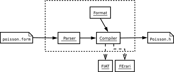
Figure 5: Diagram of the components of the form compiler FFC.

5.5 Input/output

FFC can be used either as a Python package or from the command-line. We here give a brief description of how FFC can be called from the command-line to generate C++ code for DOLFIN. To use FFC from the command-line, one specifies the form in a text file in a special language for variational forms, which is simply Python equipped with the hierarchy of classes and operators discussed above in Section 5.1. In Table 3 we give the complete code for the specification of test case 2, Poisson’s equation. Note that FFC uses tensor-notation, and thus the summation over the index i is implicit. Also note that the integral over an element $K$ is denoted by *dx.

    element = FiniteElement("Lagrange", "tetrahedron", 3)

    v = BasisFunction(element)
    u = BasisFunction(element)
    f = Function(element)
    i = Index()

    a = v.dx(i)*u.dx(i)*dx
    L = v*f*dx
    

Table 3: The complete code for specification of test case 2, Poisson’s equation, with piecewise cubics on tetrahedra in the language of FFC. Alternatively, the form can be specified in terms of standard operators: a = dot(grad(v), grad(u))*dx.

Assuming that the form has been specified in the file Poisson.form, the form can be compiled using the command ffc Poisson.form. This generates the C++ file Poisson.h to be included in a DOLFIN program. In Table 4, we include part of the output generated by FFC with input given by the code from Table 3. In addition to this code, FFC generates code for the mapping $\iota(\cdot,\cdot)$ from local to global degrees of freedom for each finite element space associated with the form. Note that the values of the $10\times 10$ element tensor $A^{K}$ (in the case of cubics on triangles) are stored as one contiguous array (block), since this is what the linear algebra backend of DOLFIN (PETSc) requires for assembly.

void eval(double block[], const AffineMap& map) const
{
  // Compute geometry tensors
  double G0_0_0 = map.det*(map.g00*map.g00 + map.g01*map.g01);
  double G0_0_1 = map.det*(map.g00*map.g10 + map.g01*map.g11);
  double G0_1_0 = map.det*(map.g10*map.g00 + map.g11*map.g01);
  double G0_1_1 = map.det*(map.g10*map.g10 + map.g11*map.g11);

  // Compute element tensor
  block[0]  =  4.249999999999996e-01*G0_0_0 + 4.249999999999995e-01*G0_0_1 +
               4.249999999999995e-01*G0_1_0 + 4.249999999999995e-01*G0_1_1;
  block[1]  = -8.749999999999993e-02*G0_0_0 - 8.749999999999995e-02*G0_0_1;
  block[2]  = -8.750000000000005e-02*G0_1_0 - 8.750000000000013e-02*G0_1_1;
  ...
  block[99] =  4.049999999999997e+00*G0_0_0 + 2.024999999999998e+00*G0_0_1 +
               2.024999999999998e+00*G0_1_0 + 4.049999999999995e+00*G0_1_1;
}
    

Table 4: Part of the code generated by FFC for the input code from Table 3.

5.6 Completing the toolchain

With the FEniCS project [Hoffman et al. (2005)], we have the beginnings of a working system realizing (in part) the Automation of Computational Mathematical Modeling, and the form compiler FFC is just one of several components needed to complete the toolchain. FIAT automates the generation of finite element spaces and FFC automates the evaluation of variational forms. Furthermore, PETSc [Balay et al. (2005b), Balay et al. (2004), Balay et al. (1997)], automating the solution of discrete systems, is used as the solver backend of FEniCS. A common C++ interface to the different FEniCS components is provided by DOLFIN.

A complete automation of CMM, as outlined in [Logg (2004)], is a major task and we hope that by a modular approach we can contribute to this automation.

6 Benchmark results

As noted above, the speedup for the code generated by the form compiler FFC can in many cases be significant. Below, we present a comparison with the standard quadrature-based approach for the test cases discussed above in Section 3.3.

The forms were compiled for a range of polynomial degrees using FFC version 0.1.6. This version of FFC does not take into account any of the optimizations discussed in Section 3.5, other than not generating code for multiplication with zero entries of the reference tensor.

For the quadrature-based code, all basis functions and their derivatives were pretabulated at the quadrature points using FIAT. Loops for all scalar products were completely unrolled.

In all cases, we have used the ”collapsed-coordinate” Gauss-Jacobi rules described by Karniadakis and Sherwin [Karniadakis and Sherwin (1999)]. These take tensor-product Gaussian integration rules over the square and cube and map them to the reference simplex. These rules are not the best known (see for example [Dunavant (1985)]), but they are fairly simple to generate for arbitrary degree. Eventually, these rules will be integrated with FIAT, but even if we reduce the number of quadrature points by a factor of five, FFC still outperforms quadrature.

The codes were compiled with gcc (g++) version 3.3.6 and the benchmark results presented below were obtained on an Intel Pentium 4 (CPU 3.0 GHz, 2GB RAM) running Debian GNU/Linux. The times reported are for the computation of each entry of the element tensor on one million elements (scaled). The total time can be obtained by multiplying with $n^{2}$, the number of entries of the element tensor. The complete source-code for the benchmarks can be obtained from the FEniCS web site [Hoffman et al. (2005)].

6.1 Summary of results

In Table 5, we summarize the results for test cases 1–4. In all cases, the speedup $T_{Q}/T_{T}$ is significant, ranging between a factor 10–1500.

From Section 4, we know that the speedup for the mass matrix should grow as $q^{d}$, but from Table 5 it is clear that the speedup is not quadratic for $d=2$ and for $d=3$, an optimum seems to be reached around $q=8$.

The reason that the predicted speedups are not obtained in practice is that the complexity estimates presented in Section 4 only account for the number of floating-point operations. When the polynomial degree $q$ grows, the number of lines of code generated by the form compiler grows. FFC unrolls all loops and generates one line of code for each entry of the element tensor to be computed. For a bilinear form, the number of entries is $n^{2}\sim q^{2d}$. With $q=8$, the number of lines of code generated is about $25,000$ for the mass matrix and Poisson in 3D, see Figure 6. As the number of lines of code grows, memory access becomes more important and dominates the run-time. Using BLAS to compute tensor products as discussed above might lead to more efficient memory traffic.

\psfrag{q}{$q$}\includegraphics[width=312.9803pt]{eps/ffc-klocs.eps}

Figure 6: Lines of code generated by the form compiler FFC as function of the polynomial degree $q$.

Note however that although the optimal speedup is not obtained, the speedup is in all cases significant, even at $q=1$.

Form	$q=1$	$q=2$	$q=3$	$q=4$	$q=5$	$q=6$	$q=7$	$q=8$
Mass 2D	12	31	50	78	108	147	183	232
Mass 3D	21	81	189	355	616	881	1442	1475
Poisson 2D	8	29	56	86	129	144	189	236
Poisson 3D	9	56	143	259	427	341	285	356
Navier–Stokes 2D	32	33	53	37	—	—	—	—
Navier–Stokes 3D	77	100	61	42	—	—	—	—
Elasticity 2D	10	43	67	97	—	—	—	—
Elasticity 3D	14	87	103	134	—	—	—	—

Table 5: Speedups $T_{Q}/T_{T}$ for test cases 1–4 in 2D and 3D.

6.2 Results for test cases

In Figures 7–10, we present the results for test cases 1–4 discussed above in Section 3.3. In connection to each of the results, we include the specification of the form in the language used by the form compiler FFC. Because of limitations in the current implementation of FFC, the comparison is made for polynomial order $q\leq 8$ in test cases 1–2 and $q\leq 4$ in test cases 3–4. Higher polynomial order is possible but is very costly to compile (compare Figure 6).

\psfrag{q}{$q$}\includegraphics[width=312.9803pt]{eps/ffc-benchmark-mass.eps}

Figure 7: Benchmark results for test case 1, the mass matrix, specified in FFC by a = v*u*dx.

\psfrag{q}{$q$}\includegraphics[width=312.9803pt]{eps/ffc-benchmark-poisson.eps}

Figure 8: Benchmark results for test case 2, Poisson’s equation, specified in FFC by a = v.dx(i)*u.dx(i)*dx.

\psfrag{q}{$q$}\includegraphics[width=312.9803pt]{eps/ffc-benchmark-navierstokes.eps}

Figure 9: Benchmark results for test case 3, the nonlinear term of the incompressible Navier–Stokes equations, specified in FFC by a = v[i]*w[j]*u[i].dx(j)*dx.

\psfrag{q}{$q$}\includegraphics[width=312.9803pt]{eps/ffc-benchmark-elasticity.eps}

Figure 10: Benchmark results for test case 4, the strain-strain term of linear elasticity, specified in FFC by a = 0.25*(v[i].dx(j) + v[j].dx(i)) * (u[i].dx(j) + u[j].dx(i)) * dx.

7 Concluding remarks and future directions

We have demonstrated a proof-of-concept form compiler that for a wide range of variational forms can generate code that gives significant speedups compared to the standard quadrature-based approach.

The form compiler FFC is still in its early stages of development but is already in production use. A number of basic modules based on FFC have been implemented in DOLFIN and others are currently being developed (Navier–Stokes and updated elasticity). This will serve as a test bed for future development of FFC.

Future plans for FFC include adding support for integrals over the boundary (adding the operator *ds to the language), support for automatic differentiation of nonlinear forms and automatic generation of dual problems and a posteriori error estimators [Eriksson et al. (1995), Becker and Rannacher (2001)], optimization through FErari [Kirby et al. (2005), SISC], [Kirby et al. (2005), BIT], adding support for new families of finite elements, including elements that require non-affine mappings from the reference element. In addition to general order continuous/discontinuous Lagrange finite elements and Crouzeix–Raviart [Crouzeix and Raviart (1973)] finite elements, the plan is to add support for Raviart–Thomas [Raviart and Thomas (1977)], Nedelec [Nédélec (1980)], Brezzi–Douglas–Marini [Brezzi et al. (1985)], Brezzi–Douglas–Fortin–Marini [Brezzi and Fortin (1991)], Taylor–Hood [Boffi (1997), Brenner and Scott (1994)], and Arnold–Winther [Arnold and Winther (2002)] elements.

Furthermore, the fact that Python is an interpreted language does impose a penalty on the performance of the compiler (but not on the generated code). However, this can be overcome by more extensive use of BLAS in numerically intensive parts of the compiler, such as the precomputation of integrals on the reference element. We also plan to investigate the use of BLAS for evaluation of tensor products as an alternative to generating explicit unrolled code. Other topics of interest include automatic verification of the correctness of the code generated by the form compiler [Kirby et al. (2005), Verification].

We wish to thank the FEniCS team, in particular Johan Hoffman, Johan Jansson, Claes Johnson, Matthew Knepley, and Ridgway Scott, for substantial suggestions and comments regarding this paper. We also want to thank one of the referees for pointing out how the tensor representation can be generalized to a quadrature-based evaluation scheme for non-affine mappings.

received

References

- Arnold and Winther (2002) Arnold, D. N. and Winther, R. 2002. Mixed finite elements for elasticity. Numer. Math. 92, 3, 401–419.
- Bagheri and Scott (2003) Bagheri, B. and Scott, R. 2003. Analysa. http://people.cs.uchicago.edu/~ridg/al/aa.html.
- Balay et al. (2004) Balay, S., Buschelman, K., Eijkhout, V., Gropp, W. D., Kaushik, D., Knepley, M. G., McInnes, L. C., Smith, B. F., and Zhang, H. 2004. PETSc users manual. Tech. Rep. ANL-95/11 - Revision 2.1.5, Argonne National Laboratory.
- Balay et al. (2005a) Balay, S., Buschelman, K., Gropp, W. D., Kaushik, D., Knepley, M. G., McInnes, L. C., Smith, B. F., and Zhang, H. 2005a. Anl anl sidl environmentsidl environment. http://www-unix.mcs.anl.gov/ase/.
- Balay et al. (2005b) Balay, S., Buschelman, K., Gropp, W. D., Kaushik, D., Knepley, M. G., McInnes, L. C., Smith, B. F., and Zhang, H. 2005b. PETSc. http://www.mcs.anl.gov/petsc/.
- Balay et al. (1997) Balay, S., Eijkhout, V., Gropp, W. D., McInnes, L. C., and Smith, B. F. 1997. Efficient management of parallelism in object oriented numerical software libraries. In Modern Software Tools in Scientific Computing, E. Arge, A. M. Bruaset, and H. P. Langtangen, Eds. Birkhäuser Press, 163–202.
- Bangerth et al. (2005) Bangerth, W., Hartmann, R., and Kanschat, G. 2005. deal.II Differential Equations Analysis Library. http://www.dealii.org.
- Becker and Rannacher (2001) Becker, R. and Rannacher, R. 2001. An optimal control approach to a posteriori error estimation in finite element methods. Acta Numerica 10, 1–102.
- Boffi (1997) Boffi, D. 1997. Three-dimensional finite element methods for the Stokes problem. SIAM J. Numer. Anal. 34, 2, 664–670.
- Brenner and Scott (1994) Brenner, S. C. and Scott, L. R. 1994. The Mathematical Theory of Finite Element Methods. Springer-Verlag.
- Brezzi et al. (1985) Brezzi, F., Douglas, Jr., J., and Marini, L. D. 1985. Two families of mixed finite elements for second order elliptic problems. Numer. Math. 47, 2, 217–235.
- Brezzi and Fortin (1991) Brezzi, F. and Fortin, M. 1991. Mixed and hybrid finite element methods. Springer Series in Computational Mathematics, vol. 15. Springer-Verlag, New York.
- Castillo et al. (2004) Castillo, P., Koning, J., Rieben, R., and White, D. 2004. A discrete differential forms framework for computational electromagnetics. Computer Modeling in Engineering and Sciences 5, 4, 331 – 346.
- Castillo et al. (2005) Castillo, P., Rieben, R., and White, D. 2005. Femster: an object-oriented class library of discrete differential forms. To appear in ACM Trans. Math. Software.
- Ciarlet (1976) Ciarlet, P. G. 1976. Numerical Analysis of the Finite Element Method. Les Presses de l’Universite de Montreal.
- Crouzeix and Raviart (1973) Crouzeix, M. and Raviart, P. A. 1973. Conforming and nonconforming finite element methods for solving the stationary stokes equations. RAIRO Anal. Num r. 7, 33–76.
- Dular and Geuzaine (2005) Dular, P. and Geuzaine, C. 2005. GetDP: a General environment for the treatment of Discrete Problems. http://www.geuz.org/getdp/.
- Dunavant (1985) Dunavant, D. A. 1985. High degree efficient symmetrical Gaussian quadrature rules for the triangle. Internat. J. Numer. Methods Engrg. 21, 6, 1129–1148.
- Eriksson et al. (1995) Eriksson, K., Estep, D., Hansbo, P., and Johnson, C. 1995. Introduction to adaptive methods for differential equations. Acta Numerica 4, 105–158.
- Eriksson et al. (1996) Eriksson, K., Estep, D., Hansbo, P., and Johnson, C. 1996. Computational Differential Equations. Cambridge University Press.
- Eriksson et al. (2003) Eriksson, K., Estep, D., and Johnson, C. 2003. Applied Mathematics: Body and Soul. Vol. III. Springer-Verlag.
- Free Software Foundation (1991) Free Software Foundation. 1991. GNU GPL. http://www.gnu.org/copyleft/gpl.html.
- Hoffman et al. (2005) Hoffman, J., Jansson, J., Johnson, C., Knepley, M., Kirby, R. C., Logg, A., and Scott, L. R. 2005. FEniCS. http://www.fenics.org/.
- Hoffman et al. (2005) Hoffman, J., Jansson, J., and Logg, A. 2005. DOLFIN. http://www.fenics.org/dolfin/.
- Hoffman and Logg (2002) Hoffman, J. and Logg, A. 2002. DOLFIN: Dynamic Object oriented Library for FINite element computation. Tech. Rep. 2002–06, Chalmers Finite Element Center Preprint Series.
- Hughes (1987) Hughes, T. J. R. 1987. The Finite Element Method: Linear Static and Dynamic Finite Element Analysis. Prentice-Hall.
- Karniadakis and Sherwin (1999) Karniadakis, G. E. and Sherwin, S. J. 1999. Spectral/ element methods for CFD. Numerical Mathematics and Scientific Computation. Oxford University Press, New York.
- Kirby (2004) Kirby, R. C. 2004. FIAT: A new paradigm for computing finite element basis functions. ACM Trans. Math. Software 30, 502–516.
- Kirby (2005) Kirby, R. C. 2005. Optimizing FIAT with the level 3 BLAS. submitted to ACM Trans. Math. Software.
- Kirby et al. (2005) Kirby, R. C., Knepley, M., Logg, A., and Scott, L. R. 2005. Optimizing the evaluation of finite element matrices. To appear in SIAM J. Sci. Comput..
- Kirby et al. (2005) Kirby, R. C., Knepley, M., and Scott, L. R. 2005. Evaluation of the action of finite element operators. submitted to BIT.
- Kirby et al. (2005) Kirby, R. C., Strout, M. M., Hovland, P., and Scott, L. R. 2005. Verification of scientific code using rationality analysis. in preparation.
- Langtangen (1999) Langtangen, H. P. 1999. Computational Partial Differential Equations – Numerical Methods and Diffpack Programming. Lecture Notes in Computational Science and Engineering. Springer.
- Logg (2004) Logg, A. 2004. Automation of computational mathematical modeling. Ph.D. thesis, Chalmers University of Technology, Sweden.
- Long (2003) Long, K. 2003. Sundance, a rapid prototyping tool for parallel PDE-constrained optimization. In Large-Scale PDE-Constrained Optimization. Lecture notes in computational science and engineering. Springer-Verlag.
- Mackie (1992) Mackie, R. I. 1992. Object oriented programming of the finite element method. Int. J. Num. Meth. Eng. 35, 425–436.
- Masters et al. (1997) Masters, I., Usmani, A. S., Cross, J. T., and Lewis, R. W. 1997. Finite element analysis of solidification using obect-oriented and parallel techniques. Int. J. Numer. Meth. Eng. 40, 2891–2909.
- Nédélec (1980) Nédélec, J.-C. 1980. Mixed finite elements in . Numer. Math. 35, 3, 315–341.
- Pironneau et al. (2005) Pironneau, O., Hecht, F., and Hyaric, A. L. 2005. FreeFEM. http://www.freefem.org/.
- Raviart and Thomas (1977) Raviart, P.-A. and Thomas, J. M. 1977. A mixed finite element method for 2nd order elliptic problems. In Mathematical aspects of finite element methods (Proc. Conf., Consiglio Naz. delle Ricerche (C.N.R.), Rome, 1975). Springer, Berlin, 292–315. Lecture Notes in Math., Vol. 606.