Quantum dynamics in ultra-cold atomic physics

Abstract

We review recent developments in the theory of quantum dynamics in ultra-cold atomic physics, including exact techniques, but focusing on methods based on phase-space mappings that are applicable when the complexity becomes exponentially large. These phase-space representations include the truncated Wigner, positive-P and general Gaussian operator representations which can treat both bosons and fermions. These phase-space methods include both traditional approaches using a phase-space of classical dimension, and more recent methods that use a non-classical phase-space of increased dimensionality. Examples used include quantum EPR entanglement of a four-mode BEC, time-reversal tests of dephasing in single-mode traps, BEC quantum collisions with up to $10^{6}$ modes and $10^{5}$ interacting particles, quantum interferometry in a multi-mode trap with nonlinear absorption, and the theory of quantum entropy in phase-space. We also treat the approach of variational optimization of the sampling error, giving an elementary example of a nonlinear oscillator.

I Introduction

Quantum dynamics is one of the most fundamental problems in modern physics. This is because time-evolution is the basis for any theoretical prediction. Yet many-body complexity makes this an extremely challenging task in quantum systems. New theoretical methods are needed, and quantitative experiments with well-understood interactions are vitally important in order to test predictions. In this article, we review some recent developments relevant to ultra-cold atomic physics.

Ultra-cold atoms provide an exceptionally simple and well-understood physical environment, allowing quantitative tests of dynamical theoretical predictions prl-84-5029 ; nat-417-529 . Recent experiments explore temperatures below $1nK$ sci-310-1513 , capable of demonstrating dynamical behavior in many-body systems in new regimes. The important new feature of these systems is that they allow isolated, macroscopic quantum systems to evolve almost unitarily, with very little coupling to external reservoirs. It is this feature of these experiments which is highly unique, and not found in most previous condensed matter experiments Datta-Electronic .

Features of recent experiments include Metcalf-Laser :

• Bose-Einstein condensates: atom ‘photons’

• Atom lasers, atomic diffraction, interferometers..

• Quantum superfluid fermions: atom ‘electrons’

• Universality: Strongly interacting fermions

• Superchemistry: Ultracold molecule formation

• Squeezed BEC: Spin-squeezing with spinor atoms

An important development is the growing ability of experimentalists to measure atomic correlations sci-310-648 and perform atom counting experiments with noise levels below the standard quantum limit of Poissonian fluctuations. A typical schematic picture is shown in Fig (1), which shows a magnetically trapped ultracold atomic cloud. After a dynamical quantum collision of two Bose condensates, the trap is turned off and atoms are counted by the multi-channel plate (MCP) sci-292-461 below the trap.

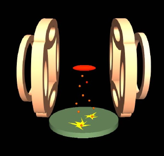
Figure 1: Schematic diagram of atom counting experiments using metastable Helium and multi-channel plate counters.

As well as these atomic correlation experiments, other experiments of interest include quantum collision prl-89-020401 and quantum interferometry experiments. In all these cases, there is an external Hamiltonian which can be changed non-adiabatically, leading to quantum dynamical evolution in the many-body system. This is obtained by externally control of laser or magnetic fields.

Unlike traditional condensed matter environments, these experiments are carried out in a high vacuum, using optical or magnetic trapping potentials. It is this feature that allows these systems to evolve with almost no contact with a heat reservoir. In summary, for the first time in physics, we have large many-body quantum systems capable of unitary evolution with a wide variety of controlled interactions. This creates an unrivaled opportunity for testing calculations of quantum dynamics.

II General Hamiltonian

The Hamiltonian of the relevant ultra-cold atomic systems usually are rather simple, being comprised of well-defined single-particle and interaction terms. Thus,

$${H}={H}_{0}+{H}_{I}\,$$ (1)

where ${H}_{0}$ and ${H}_{I}$ are the non-interacting and interacting parts of the Hamiltonian respectively, so that $H_{0}$ is a general linear Hamiltonian, given by:

$${H}_{0}=\sum_{ss^{\prime}}\int{\Psi}_{s}^{\dagger}\left(\mathbf{r}\right)\left[V_{ss^{\prime}\mathbf{r}}-\frac{\hbar^{2}\delta_{ss^{\prime}}}{2m_{s}}\nabla^{2}\right]{\Psi}_{s^{\prime}}\left(\mathbf{r}\right)d^{3}\mathbf{r}\,.$$ (2)

where ${\Psi}_{s}\left(\mathbf{r}\right)$ is a quantum field operator $\mathbf{r}$ with internal spin or atomic species index $s=1,\ldots S$, where $:\ldots:$ indicates normal ordering, and we use the Einstein summation convention for repeated indices Berezin-Method . In addition, $m_{s}$ is the mass of species $s$, $V_{ss^{\prime}\mathbf{r}}$ is a local potential, and ${H}_{I}$ describes particle-particle interactions with interaction potential $U_{ss^{\prime}\mathbf{r}\mathbf{r}^{\prime}}$ :

$${H}_{I}=\frac{1}{2}\sum_{ss^{\prime}}\int\int:\left|{\Psi}_{s}\left(\mathbf{r}\right)\right|^{2}U_{ss^{\prime}\mathbf{r}\mathbf{r}^{\prime}}\left|{\Psi}_{s^{\prime}}\left(\mathbf{r}^{\prime}\right)\right|^{2}:d^{3}\mathbf{r}d^{3}\mathbf{r}^{\prime}\,.$$ (3)

It is convenient to introduce local mode operators to treat such quantum field equationsdrummond_carter_87 . We describe this here for definiteness, although a more general mode expansion can be used. We introduce $\mathcal{M}=SM^{3}$ fermionic or bosonic annihilation operators $\tilde{\bm{a}}=\left(\tilde{a}_{\mathbf{k}s}\right)$ in momentum space, labelled by momentum $\left(\mathbf{k}=\Delta k\mathbf{j}\right)$ and spin $\left(s\right)$. Here we assume periodic boundaries in a finite volume $V=L^{3}$, and a lattice of $M^{3}$ cells, with momentum spacing of $\Delta k=2\pi/L$ in each coordinate. Localized annihilation and creation operators ${a}_{n}$ on a spatial lattice of position indices $\mathbf{r}_{\mathbf{n}}$, with cell volume $\Delta V=V/M^{3}$, are defined using a discrete Fourier transform:

$${a}_{n} =\frac{1}{M^{3/2}}\sum_{\mathbf{k}}\tilde{a}_{\mathbf{k}s}\exp\left[\frac{2\pi i\mathbf{k}\cdot\mathbf{n}}{\Delta kM}\right]$$ (4)

The combined index $n$ is a spin-space 4-vector, $n\equiv\left(\mathbf{n},s\right)$. In the case of bosonic (fermionic) fields, the commutators (anticommutators) are defined as:

$$\left[{a}_{m},{a}_{n}^{\dagger}\right]_{\pm} = \delta_{mn}^{4}$$

$$\left[{a}_{m},{a}_{n}\right]_{\pm} = 0\,\,.$$ (5)

The corresponding local number operator is ${N}_{m}={a}_{m}^{\dagger}{a}_{m}$. The continuum Hamiltonian is regained in the limit of a large number of lattice sites of the resulting Hubbard type model Hamiltonian:

$${H}({\bm{a}}^{\dagger},{\bm{a}})=\lim_{\Delta V\rightarrow 0}\hbar\sum_{nn^{\prime}}\left[\omega_{nn^{\prime}}{a}_{n}^{\dagger}{a}_{n^{\prime}}+\frac{1}{2}\chi_{nn^{\prime}}:{N}_{n}{N}_{n^{\prime}}:\right]\,.$$ (6)

In the uniform case, the hopping matrix $\omega_{nn^{\prime}}$ is

$$\omega_{nn^{\prime}}=\frac{\hbar}{2m_{s}}\sum_{\mathbf{k}}\mathbf{k}^{2}\exp\left[\frac{2\pi i\mathbf{k}\cdot\left(\mathbf{n}-\mathbf{n}^{\prime}\right)}{\Delta kM}\right]\delta_{ss^{\prime}}$$ (7)

and the interaction matrix $\chi_{\mathbf{mn}}$ is (approximately):

$$\hbar\chi_{nn^{\prime}}=U_{ss^{\prime}\mathbf{r}_{\mathbf{n}}\mathbf{r}_{\mathbf{n}^{\prime}}}\,.$$

While this is introduced here as an approximation to a continuum system, it is also experimentally feasible to use an optical lattice prl-82-2022 ; jpb-35-3095 to engineer the hamiltonian directly, so that each spatial index coincides with a local trapping potential well. In this way one can obtain a physical system directly corresponding to the famous Hubbard model of condensed matter rsa-276-238 , except that it does not involve the numerous approximations that would be required in a typical condensed matter setting. In the following calculations, we will assume for simplicity that the interaction is local in space, with $\chi_{nn^{\prime}}=\chi_{ss^{\prime}}\delta_{\mathbf{nn^{\prime}}}^{3}$; although this is not essential.

II.1 Exponential complexity

The central issue that makes quantum dynamical calculations difficult in many body quantum physics is the issue of exponential complexity itp-21-467 . For example, if we consider $N$ bosons distributed among $\mathcal{M}$ modes, the number of distinct orthogonal quantum states is obtained by combinatorics: how many ways can we divide the particles amongst the modes? The number of quantum states is then simply:

$$N_{B}=\frac{(\mathcal{M}+N-1)!}{(\mathcal{M}-1)!N!}$$ (8)

To give relevant numbers, suppose we consider numbers that are approximately typical of many ultra-cold atom experiments, with $N=\mathcal{M}=500,000$. One finds that:

$$N_{B}\approx 2^{2\mathcal{M}}\approx 10^{300,000}$$ (9)

With fermions, we have fewer states, since each mode can have an occupation number of $0$ or 1, meaning that:

$$N_{F}\approx 2^{\mathcal{M}}\approx 10^{150,000}$$ (10)

In either case, there are more linear equations to solve than atoms in the universe. By comparison, the number of classical equations would be

$$N_{C}=2\mathcal{M}=10^{6}$$ (11)

While the classical problem is difficult, it is soluble on many current digital computers. The quantum problem, on the other hand, is nearly impossible to treat. In particular, one can’t diagonalize the Hamiltonian, which is now a $10^{300,000}\times 10^{300,000}$ matrix in the bosonic case.

III Exact dynamics

If there are small numbers of modes, one can indeed obtain exact eigenvectors. In this case it is possible to diagonalize the Hamiltonian, and obtain the eigenvectors and eigenvalues for a small number of particles, typically in the range $10-100$. As an example, we consider the generation of entanglement through four-mode nonlinear dynamics in two-well trap holding a two-species BEC systems, in which the nonlinearity enters through S-wave scattering interactions EPR . The basic interaction that generates entanglement in the first place is the nonlinear S-wave scattering interaction, which we consider to be an interaction between two spin-states in ${}^{87}Rb$. The two spin states labeled $i=1,2$ are $|1\rangle\equiv|F=1,\,m_{F}=+1\rangle,\ |2\rangle\equiv|F=2,\,m_{F}=-1\rangle$, and there are two spatial modes corresponding to optical trapping of modes labeled $a,b$ for clarity. Thus, $S=2$, $M=2$ and $\mathcal{M}=SM=4$. With such a small number of modes there is no exponential complexity issue, and the Hamiltonian can be exactly diagonalized using numerical techniques.

The Hamiltonian for the coupled system is:

$${H}/\hbar=\omega\sum_{i}{a}_{i}^{\dagger}{b}_{i}+\frac{1}{2}\left[\sum_{ij}\chi_{ij}{a}_{i}^{\dagger}{a}_{j}^{\dagger}{a}_{j}{a}_{i}\right]+\left\{{a}_{i}\leftrightarrow{b}_{i}\right\}\,.$$ (12)

Here $\omega$ is the inter-well tunneling rate between the two wells with localized modes ${a}_{i},{b}_{i}$ while $\chi_{ij}$ is the intra-well interaction matrix between the different spin components.

We can solve this using either Schroedinger or Heisenberg equations of motion. To illustrate this, suppose that $\omega=0$, and we have just one well. In the Heisenberg case, one obtains:

$$\frac{d{a}_{i}}{dt} = \frac{i}{\hbar}\left[{H},{a}_{i}\right]$$ (13)

$$= -i\sum_{j}\chi_{ij}{N}_{j}{a}_{i}.$$

Since the number of particles is conserved in each mode, this has the solution:

$${a}_{i}\left(t\right) = \exp\left[-i\sum_{j}\chi_{ij}{N}_{j}t\right]{a}_{i}\left(0\right)$$ (14)

More generally, it is convenient to use a matrix expansion of the Hamiltonian in a number-state basis. For dynamics, we explicitly assume that ${a}_{1},\ b_{1}$ and $a_{2},\ b_{2}$ are initially in coherent states. This models the relative coherence between the wells obtained with a low inter-well potential barrier, together with an overall Poissonian number fluctuation as typically found in an experimental BEC. We note that the coherent state also includes an overall phase coherence, which has no effect on our results. For simplicity, we suppose that the initial state is prepared in an overall four-mode coherent state using a Rabi rotation: $|\psi>=|\alpha>_{{a}_{1}}|\alpha>_{b_{1}}|\alpha>_{a_{2}}|\alpha>_{b_{2}}$.

Next, we assume that the inter-well potential is increased so that each well evolves independently. Finally, we decrease the inter-well potential for a short time, so that it acts as a controllable, non-adiabatic beam-splitter olsen , to allow interference between the wells, followed by independent spin measurements in each well.

III.1 Squeezed and entangled states produced by double-well BEC

We now use the techniques given above to investigate a particular dynamical strategy for generating EPR entanglement. The technique treated here is generally along the lines investigated experimentally in fibre-optics, by comparison with squeezing and entanglement experiments in optical fibers fiberexperimentNature ; FiberEntangle ; FiberEntangleLeuchs . An important difference is that the fiber experiments use time-delayed pulses to eliminate interactions between the components. This is not readily feasible in BEC experiments, although Feshbach resonances can achieve this to some extent.

Let ${a}_{1},$$a_{2}$ be operators for two internal states in the $A$ well and $b_{1}$ , $b_{2}$ operators for two internal states at the $B$ well. $N_{A}=a_{2}^{\dagger}a_{2}+{a}_{1}{a}_{1}$ and $N_{B}=b_{2}^{\dagger}b_{2}+b_{1}^{\dagger}b_{1}$ are the atom number operators of these modes in each well. We define Schwinger spin operators at each site for the measurement of the EPR paradox and entanglement. We define general, phase-rotated spin components according to:

$$J_{x}^{A} = \left(a_{2}^{\dagger}{a}_{1}e^{i(\theta_{2}-\theta_{1})}+{a}_{1}a_{2}e^{-i(\theta_{2}-\theta_{1})}\right)/2\ ,$$

$$J_{y}^{A} = \left(a_{2}^{\dagger}{a}_{1}e^{i(\theta_{2}-\theta_{1})}-{a}_{1}a_{2}e^{-i(\theta_{2}-\theta_{1})}\right)/2i\ ,$$

$$J_{z}^{A} = \left(a_{2}^{\dagger}a_{2}-{a}_{1}{a}_{1}\right)/2\$$ (15)

at $A$ and similar definition at $B$, while $\Delta\theta=\theta_{2}-\theta_{1}$ is the phase shift between mode $1$ and mode $2$.

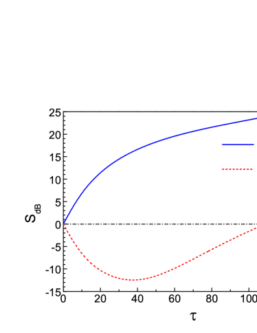
Figure 2: Squeezing of Schwinger spin operators $10log_{10}\left(\Delta^{2}J_{\theta}/n_{0}\right)$ (solid), $10log_{10}\left(\Delta^{2}J_{\theta+\pi/2}/n_{0}\right)$ (dashed), and shot noise level $n_{0}=|\langle J_{y}\rangle|/2$ (dash-dotted) via BEC with number of $Rb$ atoms. Here the parameters correspond to $Rb$ atoms at magnetic field $B=9.131G$, with scattering lengths ${a}_{1}=100.4a_{0}$, $a_{22}=95.5a_{0},$ and ${a}_{1}=80.8a_{0}$. $a_{0}=53pm$. The coupling constant $\chi_{ij}\propto 2\text{\leavevmode{w}}_{\perp}a_{ij}$. Here $N_{A}=200$, $\tau=\chi_{11}N_{A}t$.

We the select the phase shift to make sure $\langle J_{y}\rangle\neq 0$. The Schwinger spin operators orthogonal to $J_{y}$ are given as $J(\theta)=cos(\theta)J_{z}+sin(\theta)J_{x}$, all of which have the property $\langle J(\theta)\rangle=0$. We define $\Delta\theta=\pi/2-\alpha$ where $\alpha$ is time dependent, such that $\langle a_{2}^{\dagger}{a}_{1}\rangle=|\langle a_{2}^{\dagger}{a}_{1}\rangle|e^{i\alpha}$. This plane contains an infinite family of maximally conjugate Schwinger spin operators, generally given by $J(\theta)$ and $J(\theta+\pi/2)$ which obey the uncertainty relation

$$\Delta^{2}J(\theta)\Delta^{2}J(\theta+\pi/2)\geq|\langle J_{y}\rangle|^{2}/4\ .$$ (16)

Thus a state which obeys

$$\Delta^{2}J(\theta)<|\langle J_{y}\rangle|/2<\Delta^{2}J(\theta+\pi/2)$$ (17)

is a squeezed state, as shown in the Fig. 2. Here, we have optimized the phase choice $\theta$ to get the best squeezing of the Schwinger spin operators by the criterion that $\partial\Delta^{2}J(\theta)/\partial\theta=0$, hence obtaining

$$tg(2\theta)=2\langle J_{z},\ J_{x}\rangle/(\Delta^{2}J_{z}-\Delta^{2}J_{x}).$$ (18)

In this strategy, spin-squeezing at each site can be readily obtained, by unitary evolution from an initial coherent state, under the local Hamiltonian. Then we can obtain sum and difference spins between two sites: $\Delta^{2}{J}_{\theta\pm}^{AB}=\Delta^{2}({J}_{\theta}^{A}-{J}_{\theta}^{B})$ and $\Delta^{2}{J}_{(\theta+\pi/2)\pm}^{AB}=\Delta^{2}({J}_{\theta+\pi/2}^{A}+{J}_{\theta+\pi/2}^{B})$, prior to using the beam-splitter - which is achieved by a modulation of the inter-well potential, as shown in Fig. 3(a).

After using the beam-splitter, entanglement can be detected via spin measurements using the spin version of the Heisenberg-product entanglement criterion FiberEntangle

$$E_{product}=\frac{2\sqrt{\Delta^{2}{J}_{\theta\pm}^{AB}\cdot\Delta^{2}{J}_{(\theta+\pi/2)\pm}^{AB}}}{|\langle{J}_{y}^{A}\rangle|+|\langle{J}_{y}^{B}\rangle|}<1\,,$$ (19)

or the sum criterion BowenPolarizationEnt

$$E_{sum}=\frac{\Delta^{2}{J}_{\theta\pm}^{AB}+\Delta^{2}{J}_{(\theta+\pi/2)\pm}^{AB}}{|\langle{J}_{y}^{A}\rangle|+|\langle{J}_{y}^{B}\rangle|}<1\,.$$ (20)

as shown in Fig. 3(b).

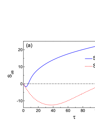
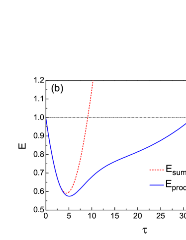
Figure 3: (a) Squeezing of Schwinger spin operators $S_{dB}$: $S_{+}=10\,log_{10}\left[\Delta^{2}({J}_{\theta}^{A}-{J}_{\theta}^{B})/n_{0}\right]$ (solid), $S_{-}=10\,log_{10}\left[\Delta^{2}({J}_{\theta+\pi/2}^{A}+{J}_{\theta+\pi/2}^{B})/n_{0}\right]$ (dashed), and $n_{0}=(|\langle{J}_{y}^{A}\rangle|+|\langle{J}_{y}^{B}\rangle|)/2$ is shot noise (dash-dotted). (b) Entanglement ($E_{product}$) based on the criterion (19) by the solid curve and $E_{sum}$ in sum criterion (20) by the dashed curve. (This figure has been published in Ref. EPR )

While diagonalization is possible for even larger particle numbers, the two-mode approximation becomes less and less reliable. For larger numbers of particles the interaction energy becomes as large as as the harmonic oscillator mode spacing. This means that few mode approximations become inapplicable, and the problem quickly develops exponentially large numbers of many-body states. Methods for treating this more general case are given in the next section.

IV Classical phase-space

Early techniques for calculating the dynamics and thermal equilibrium states of large quantum systems used techniques based on mappings to a classical phase-space Gardiner-Quantum . These were used not just in statistical many-body theory, but also in applications involving coherence theory and lasers. The most widely used methods of this type are the Wigner representationwigner_32 and the Glauber-Sudarshan glauber_63 ; sudarshan_63 P-representations. These differ in some technical details. In essence, both can be used for mapping second-quantized bosonic fields to a classical phase-space. However, the Wigner representation corresponds to symmetrically-ordered operator mappings, while the P-representation corresponds to normal ordering. It is also possible to use an anti-normal ordered mapping, called the Husimi Q-function husimi_40 , but this is less commonly used for dynamical calculations. When used for quantum fields, in a truncation approximation described below, these types of phase-space method are sometimes called c-field techniques. Phase-space methods for quantum fields were used to predict quantum squeezing in solitons in fiber optics carter_drummond_87 ; carter_drummond_91 ; drummond_hardman_93 ; drummond_shelby_93 ; Drummond2001a , with an excellent agreement with subsequent experimental testsRosenbluh1991a ; Heersink2005a ; corney_drummond_06a . They were later applied to ultra-cold atomic BEC dynamics steel_olsen_98 , and have been widely used, especially at finite temperatures blakie_bradley_08 ; Egorov2011 .

IV.1 Glauber-Sudarshan P-representation

This approach uses an overcomplete set of coherent states prx-131-2766 ; pra-59-1538 , parameterized by a complex vector $\bm{\alpha}$:

$$\left|\bm{\alpha}\right\rangle=\exp\left[\bm{a}^{\dagger}\cdot\bm{\alpha}-\bm{\alpha}^{*}\cdot\bm{\alpha}/2\right]\left|\bm{0}\right\rangle$$ (21)

and one then obtains an expansion for the density matrix in the form:

$${\rho}=\int P(\bm{\alpha}){\Lambda}_{1}\left(\bm{\alpha}\right)d^{2M}\bm{\alpha}$$ (22)

where ${\Lambda}_{1}\left(\bm{\alpha}\right)$ is a diagonal coherent state projection operator, which is the basis for the expansion, defined as:

$${\Lambda}_{1}\left(\bm{\alpha}\right)=\left|\left(-\right)\bm{\alpha}\right\rangle\left\langle\bm{\alpha}\right|$$ (23)

Here we note that the same expansion can be used for either fermions of bosons. In the case of fermions, $\bm{\alpha}$ is a Grassmann variableBerezin-Method , and one must use the bracketed minus sign in Eq (23). This representation generates normal-ordered operator products, in the sense that moments of $P(\bm{\alpha})$ correspond directly to expectation values of normally ordered operator products.

The advantage of this approach is that it maps quantum states into $\mathcal{M}$ complex coordinates, $\bm{\alpha}=\mathbf{p}+i\mathbf{x},$ and hence only has classical complexity. Another advantage is that the use of normally-ordered products means that there is no UV vacuum divergence in the expectation values. However, for many quantum states, including all entangled states, the distribution is not positive, and indeed is highly singular.

In the bosonic case, the operator basis can be written in an alternative form pra-68-63822 , as:

$${\Lambda}_{s}(\bm{\lambda})=\left[\frac{2}{1+s}\right]^{\mathcal{M}}:\exp\left[-2\delta{\bm{a}}^{\dagger}\delta{\bm{a}}/\left(1+s\right)\right]:\,,$$ (24)

where $\delta{\bm{a}}={\bm{a}}-\bm{\alpha}$ , $\delta{\bm{a}}^{\dagger}={\bm{a}}^{\dagger}-\bm{\alpha}^{*}$ are relative displacements, and $s$ indicates the operator ordering Cahill1969 . Here $s=1$ is used for normal ordering, as in the case of the P-representation, and other orderings are treated in the next subsection. This allows us to recognize that the basis is just a Gaussian function of the mode operators: an exponential of a quadratic function of annihilation and creation operators. Just as with similar Gaussian bases for ordinary complex functions, such an operator basis has more than one possible form, obtained by changing the variance.

IV.2 Wigner-Moyal phase-space

An even older phase-space method was developed by Wigner wigner_32 , who treated thermal equilibrium problems, and Moyal moyal_49 , who extended this to a full dynamical equivalence with quantum mechanics. This can also be written as an expansion over a Gaussian operator basis with symmetric ordering mappings, so that $O=0$ . This reduces the basis variance, and therefore increases the variance of the distribution function. Formally, the expansion is written as:

$$\,{\rho}=\int W(\bm{\alpha}){\Lambda}_{0}\left(\bm{\alpha}\right)d^{2\mathcal{M}}\bm{\alpha}$$ (25)

This type of distribution generates symmetrically ordered operator products. It maps quantum states into $\mathcal{M}$ complex or $2\mathcal{M}$ real coordinates, and has the advantage that this mapping gives dynamical equations that are the most similar to classical behavior. Historically, Moyal first showed how to map quantum operators into differential equations, and had a famous correspondence with Dirac, who objected to the fact that the distribution had no probabilistic interpretation.

As result, there is a problem for computational implementation. One would like to sample the Wigner distribution probabilistically, but this is not always possible. Since the mapping is nonpositive, there is no generally efficient and accurate sampling procedure. The representation is also typically UV divergent in three dimensions, due to vacuum field fluctuations of symmetrically ordered moments.

For the case of an initial coherent state,

$$\left|\Psi_{0}\right\rangle=\left|\bm{\alpha}_{0}\right\rangle$$ (26)

the initial Wigner distribution is Gaussian and positive, so that the quantum noise can be readily sampled stochastically, with:

$$\bm{\alpha}=\bm{\alpha}_{0}+\delta\bm{\alpha}_{0}$$ (27)

where $\delta\bm{\alpha}_{0}$ is a Gaussian random complex number, such that the only nonvanishing correlations are:

$$\left\langle\delta\bm{\alpha}_{0}\delta\bm{\alpha}_{0}^{*}\right\rangle=\frac{1}{2}\,.$$ (28)

For more general states - even as simple as a number state - the Wigner distribution exists but has no stochastic equivalent. The quantum dynamical manifestation of this problem is that one obtains a third-order Fokker-Planck equation for the Wigner time evolution when there are nonlinear Hamiltonian terms. Such an equation has no stochastic equivalent, unless truncated to give a second order differential equation. In this approximation, the resulting equation has a semi-classical form, with:

$$i\frac{d\alpha_{m}}{dt}=\sum_{n}\left[\omega_{mn}\alpha_{n}+\chi_{mn}\left|\alpha_{n}\right|^{2}\alpha_{m}\right]$$ (29)

While apparently classical, this equation includes quantum noise in the initial conditions, and can simulate nonclassical entangled states, in an approximation which is valid in the limit of large mode occupations

It was the nonpositivity of the Wigner representation that led Feynman to make his famous conjectureitp-21-467 that it was not possible to use a classical or digital computer to make a probabilistic representation of a quantum system. Nevertheless, while not exact, the truncated Wigner approach is relatively simple, and has useful applications as a practical approximation when mode occupation numbers are large.

We note that the Husimi Q-function husimi_40 , which corresponds to antinormal ordering with $O\rightarrow-1$, is always positive. Yet, paradoxically, this has no direct stochastic equivalent either, since the corresponding Fokker-Planck equation is not positive-definite. As we show in the next section, despite Feynman’s remark, there are routes to positive representations of quantum systems that do have stochastic equivalents, but they involve enlarged, non-classical phase-space mappings.

IV.3 Large-scale two-component atom interferometry

As an illustration of the Wigner phase-space techniques, consider interferometry of a two-component ⁸⁷Rb BEC in a harmonic trap, which is performed by many experimental groups worldwide. Atom numbers in these experiments range from $10^{4}$ to $10^{6}$, which makes it impossible to simulate the behavior of the system exactly in a few mode approximation: these larger traps are inherently multi-mode. A common approach involves the propagation of semi-classical Gross-Pitaevskii equations Gardiner-Quantum . Although these equations provide a good description of the condensate evolution, they do not account for quantum effects in the cloud, and cannot predict variances of the observables. A truncated Wigner phase-space approach can be used to obtain more accurate predictions europhys-lett-21-279 ; pra-58-4824 ; jpb-35-3599 .

The effective Hamiltonian in three dimensions is

$${H}/\hbar=\sum_{ss^{\prime}}\int d^{3}\mathbf{\mathbf{x}}\left\{{\Psi}_{s}^{\dagger}K_{ss^{\prime}}{\Psi}_{s^{\prime}}+\frac{\chi_{ss^{\prime}}}{2}{\Psi}_{s}^{\dagger}{\Psi}_{s^{\prime}}^{\dagger}{\Psi}_{s^{\prime}}{\Psi}_{s}\right\},$$ (30)

where ${\Psi}_{s}$ is an annihilation operator for spin $s$, with the space position omitted for brevity, and $\chi_{ss^{\prime}}$ is the spin-dependent contact interaction strength. The operator $K_{ss^{\prime}}$ is the single-particle Hamiltonian:

$$K_{ss^{\prime}}=\left(-\frac{\hbar}{2m}\nabla^{2}+\omega_{s}+V_{s}(\mathbf{x})/\hbar\right)\delta_{ss^{\prime}}+\tilde{\Omega}_{ss^{\prime}}(t),$$ (31)

where $m$ is the atomic mass, $V_{s}$ is the external trapping potential for spin $s$, $\omega_{s}$ is the internal energy of spin $s$, $\tilde{\Omega}_{ss^{\prime}}$ is the time-dependent coupling term. Losses, which can play a significant part in the evolution, can be included into the model by adding a loss term to the master equation prl-89-140402 :

$$\frac{d{\rho}}{dt}=-\frac{i}{\hbar}\left[{H},{\rho}\right]+\sum_{n,\mathbf{l}}\kappa_{\mathbf{l}}^{(p)}\int d^{D}\mathbf{x}\mathcal{L}_{\mathbf{l}}^{(p)}\left[{\rho}\right],$$ (32)

where $p$ is the number of the interacting particles in the loss process, the vector $\mathbf{l}$ specifies the number of particles with each spin participating in the interaction, and $\mathcal{L}$ is the operator functional:

$$\mathcal{L}_{\mathbf{l}}^{(p)}\left[{\rho}\right]=2{O}_{\mathbf{l}}^{(p)}{\rho}{O}_{\mathbf{l}}^{(p)\dagger}-{O}_{\mathbf{l}}^{(p)\dagger}{O}_{\mathbf{l}}^{(p)}{\rho}-{\rho}{O}_{\mathbf{l}}^{(p)\dagger}{O}_{\mathbf{l}}^{(p)}.$$ (33)

The reservoir coupling operators ${O}_{\mathbf{l}}^{(p)}$ are the distinct $p$-fold products of local field annihilation operators,

$${O}_{\mathbf{l}}^{(p)}={O}_{\mathbf{l}}^{(p)}({\mathbf{\Psi}})={\Psi}_{l_{1}}(\mathbf{x}){\Psi}_{l_{2}}(\mathbf{x})\ldots{\Psi}_{l_{p}}(\mathbf{x}),$$ (34)

describing local collisional losses.

After a transformation to the Wigner representation using functional Wigner correspondences pra-58-4824 and truncation of high-order terms, the resulting equations take a form similar to that of coupled GPEs with the addition of stochastic terms Egorov2011 :

$$\frac{d\phi_{s}(\mathbf{x})}{dt} =-i\sum_{u}\left(K_{su}\phi_{u}+U_{su}|\phi_{u}|^{2}\phi_{s}\right)$$

$$-\Gamma_{s}(\mathbf{x})+\sum_{p,\mathbf{l}}\beta_{\mathbf{l},s}^{(p)}\zeta_{\mathbf{l}}^{(p)}(\mathbf{x},t),$$ (35)

where $\phi_{s}(\mathbf{x})$ is a Wigner c-field corresponding to the operator field $\Psi_{s}(\mathbf{x})$. Additionally, $\Gamma_{s}$ is the nonlinear loss term and $\beta_{\mathbf{l},s}^{(p)}$ is the damping noise coefficient which are both functions of the Wigner fields, while $\zeta_{\mathbf{l}}^{(p)}(\mathbf{x},t)$ is a corresponding complex, stochastic delta-correlated Gaussian noise such that:

$$\left\langle\zeta_{\mathbf{l}}^{(p)}(\mathbf{x},t)\zeta_{\mathbf{k}}^{(p^{\prime})*}(\mathbf{x}^{\prime},t^{\prime})\right\rangle=\delta_{\mathbf{l}\mathbf{k}}\delta_{pp^{\prime}}\delta^{D}\left(\mathbf{x}-\mathbf{x}^{\prime}\right)\delta\left(t-t^{\prime}\right).$$ (36)

These stochastic equations can be solved numerically using conventional methods on a discrete lattice. The resulting equations then have a similar form to the general lattice Wigner equations, Eq (29), apart from additional loss and noise terms:

$$\frac{d\alpha_{m}}{dt} =-i\sum_{n}\left[\omega_{mn}\alpha_{n}+\chi_{mn}\left|\alpha_{n}\right|^{2}\alpha_{m}\right]$$

$$-\Gamma_{m}+\sum_{p,\mathbf{l}}\beta_{\mathbf{l},s}^{(p)}\zeta_{\mathbf{l},m}^{(p)}(t),$$ (37)

Correlations of any order can be extracted, and specifically, one can obtain the value of squeezing parameter $\xi^{2}$. This serves as an indicator of entanglement in the condensate nat-409-63 ; pra-50-67 :

$$\xi^{2}=\frac{N\Delta{S}_{min}^{2}}{\langle{S}\rangle^{2}},$$ (38)

where $N$ is the number of atoms, ${S}$ is the total spin, and $\Delta{S}_{min}^{2}$ is the minimal variance of spin over all possible directions. The squeezing parameter is a fourth-order field correlation, with values $\xi^{2}<1$ indicating entangled, or spin squeezed states. By simulating the evolution of the condensate under different conditions one can find the optimal regime for producing maximum squeezing.

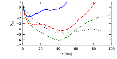
Figure 4: Wigner simulations of squeezing in the vicinity of $9.1\,\mathrm{G}$ Feshbach resonance in ⁸⁷Rb plotted with a logarithmic scale $S_{dB}=10\,log_{10}(\xi^{2})$. Inter-component scattering lengths: ${a}_{1}=80.0\,a_{0}$ (blue solid line), ${a}_{1}=85.0\,a_{0}$ (red dashed line), ${a}_{1}=90.0\,a_{0}$ (green dash-dotted line) and ${a}_{1}=95.0\,a_{0}$ (black dotted line).

For example, the inter-component scattering length of optically trapped two-component ⁸⁷Rb condensate of states $|F=1,\,m_{F}=+1\rangle$ and $|F=2,\,m_{F}=-1\rangle$ near a Feshbach resonance at $9.1\,\mathrm{\mathrm{G}}$ can be changed by varying the strength of magnetic field. When one moves closer to the resonance, the inter-component scattering length decreases, providing better squeezing, but inter-component losses increase correspondingly pra-80-050701 , eliminating the coherence faster. Fig (4) shows the evolution of squeezing parameter in time for four different values of ${a}_{1}$, where best results are achieved for ${a}_{1}=90\,a_{0}$. In other words, one has to pick an optimal but non-zero detuning from the Feshbach resonance in order to get maximum squeezing.

V Non-classical phase-space

We generically regard any expansion of the density matrix in a complete, non-orthogonal basis set with continuous variables as a phase-space method. Such methods are not restricted to classical mappings, however. In the following sections, we review progress in developing non-classical phase-space mappings, typically using higher than classical dimensionality. This approach is essentially a middle ground between the low complexity of classical phase-space, and the exponentially large complexity of the full many-body Hilbert space.

V.1 Positive-P function methods

In this approach, one extends the mapping of a bosonic field theory onto classical phase-space used in the Glauber-Sudarshan P-function, to a larger phase-space of double the classical dimension. This is best thought of as a minimal prescription for including coherent state superpositions and entanglement into the basis set. Thus, one defines:

$${\rho}=\int P_{+}(\bm{\alpha},\bm{\beta}){\Lambda}_{+}\left(\bm{\alpha},\bm{\beta}\right)d^{2M}\bm{\alpha}d^{2M}\bm{\beta}$$ (39)

where the basis set is now:

$${\Lambda}_{+}\left(\bm{\alpha},\bm{\beta}\right)=\frac{\left|\bm{\alpha}\right\rangle\left\langle\bm{\beta}^{*}\right|}{\left\langle\bm{\beta}^{*}\right|\left|\bm{\alpha}\right\rangle}$$ (40)

This enlarged phase-space allows positive probabilities for any quantum state, since it is possible to prove an existence theorem that any physical density matrix has a positive distribution in this form. While this itself is no different to the properties of the Husimi Q-function - another positive representation - there are additional advantages, as we explain below. In comparison to the usual diagonal Glauber-Sudarshan case, we note that the +P representation has these differences:

• It now maps quantum states into 4M real coordinates: $\bm{\alpha},\bm{\beta}=\mathbf{p}+i\mathbf{x},\,\,\mathbf{p}^{\prime}+i\mathbf{x}^{\prime}$

• The corresponding phase-space has double the dimensionality of a classical phase-space

• The advantage is that one can represent superpositions including entangled states without singularities.

V.2 +P Existence Theorem

The most significant property of the +P method is the existence theorem: a positive P-function always exists, for any density matrix. While the proof is too lengthy to be given here, we quote the result, which has a simple constructive form drummond_gardiner_1980 . For any hermitian, positive-definite density matrix ${\rho}$, there is a corresponding positive-P distribution, of ‘canonical’ form:

$$P_{+}(\boldsymbol{\alpha},\boldsymbol{\beta})=\left[\frac{1}{4\pi^{2}}\right]^{\mathcal{M}}e^{-\left|\boldsymbol{\alpha}-\boldsymbol{\beta}^{*}\right|^{2}/4}\left\langle\frac{\boldsymbol{\alpha}+\boldsymbol{\beta}^{*}}{2}\right|{\rho}\left|\frac{\boldsymbol{\alpha}+\boldsymbol{\beta}^{*}}{2}\right\rangle$$ (41)

The advantage here is not just that the distribution is nonsingular, but more importantly that probabilistic sampling is possible. This is a crucial issue when dealing with the complexity of many-body systems. Generally, random, probabilistic sampling is the only practical approach for subduing the unruly nature of an exponentially complex Hilbert space.

This approach nevertheless is not without its own problems. The use of a non-orthogonal basis means that the distribution is non-unique. We can choose a compact form - like the ‘canonical’ positive form given above - as an initial condition. However, this form is generally not conserved by the equations of motion, since it is not unique. If the equations of motion generate distributions that are less compact as time evolves, the this allows sampling errors to grow with time.

An important application of the +P distribution is the calculation of measurable operator moments. In order to calculate an operator expectation value, there is a correspondence between the moments of the +P distribution, and the normally ordered operator products. These come directly from the fact that coherent state are eigenstates of the annihilation operator, and that $\mathrm{{Tr}}\left[{\Lambda_{+}}(\boldsymbol{\alpha},\boldsymbol{\beta})\right]=1$, which means that any normally ordered operator product is simply a stochastic average of the phase-space variables:

$$\langle{a}_{m}^{\dagger}\cdots{a}_{n}\rangle =\mathrm{{Tr}}\left[\cdots{a}_{n}{\Lambda_{+}}(\boldsymbol{\alpha},\boldsymbol{\beta}){a}_{m}^{\dagger},\ldots\right]$$ (42)

$$=\int\int P_{+}(\boldsymbol{\alpha},\boldsymbol{\beta})[{\beta}_{m}\cdots{\alpha}_{n}]d^{2\mathcal{M}}\boldsymbol{\alpha}\,d^{2\mathcal{M}}\boldsymbol{\beta}$$

V.3 +P time-evolution

The route to obtaining time-evolution equations is to map operator equations into differential equations for the P-function. Differentiating the +P projection operator gives the following four identities:

$${a}_{m}^{\dagger}{\Lambda} = \left[\frac{\partial}{\partial\alpha_{m}}+\beta_{m}\right]{\Lambda}$$

$${a}_{m}{\Lambda} = \alpha_{m}{\Lambda}$$

$${\Lambda}{a}_{m} = \left[\frac{\partial}{\partial\beta_{m}}+\alpha_{m}\right]{\Lambda}$$

$${\Lambda}{a}_{m}^{\dagger} = \beta_{m}{\Lambda}$$ (43)

Since the projector is an analytic function of both $\alpha^{m}$ and $\beta^{m}$, we can obtain alternate identities by replacing $\partial/\partial\alpha$ by either $\partial/\partial\alpha_{x}$ or $\partial/i\partial\alpha_{y}$. This equivalence allows a positive-definite diffusion to be obtained, with stochastic evolution. The result of this procedure is that our exponential complex quantum problem is now transformed into a stochastic equation. Thus, for the case of a single-component Bose gas with S-wave interactions, one obtains the following equations in the simplest case:

$$i\frac{d\alpha^{m}}{dt} = \omega_{mn}\alpha_{n}+\left[\chi\alpha_{m}\beta_{m}+\sqrt{i\chi}\ \xi_{m}^{(1)}\left(t\right)\right]\alpha_{m}$$ (44)

$$-i\frac{d\beta_{m}}{dt} = \omega_{mn}\beta_{n}+\left[\chi\alpha_{m}\beta_{m}+\sqrt{-i\chi}\ \xi_{m}^{(2)}\left(t\right)\right]\beta_{m}$$

Here $\xi_{m}^{(i)}\left(t\right)$ are 2M independent real, random Gaussian noise terms, with correlations given on a discrete spatial lattice with cell volume $\Delta V$, by:

$$\left\langle\xi_{m}^{(i)}\left(t\right)\xi_{m^{\prime}}^{(i^{\prime})}\left(t^{\prime}\right)\right\rangle =\frac{1}{\Delta V}\delta_{mm^{\prime}}\delta_{ii^{\prime}}\delta\left(t-t^{\prime}\right).$$ (45)

Similar techniques can also be used for the case of fermions, using the Gaussian representation method, with some modifications which are not treated in detail here. In both cases, the essential trade-off is that, as with any sampling technique, many parallel trajectories are needed to control growing sampling errors. This can be modified by changing the choice of basis, and the stochastic mapping which is not unique. This approach leads to the idea of a ‘stochastic gauge’job-5-S281 , which multiplies the basis operator ${\Lambda_{+}}$ by a random weight $\Omega$, and improves convergence properties by reducing the sampling error.

We emphasize that while any stochastic method only converges for a large number of samples, the sampling error is generally a well-controlled numerical error. Like the momentum cut-off, the sample-size can be changed and the error monitored using well-defined numerical procedures.

V.4 Time-reversal tests

We now consider two examples of the application of the +P distribution to quantitative simulations of time-evolution under our Hubbard-type Hamiltonian.

By choosing a modified stochastic gauge, it is possible to simulate a very large number of bosons, and verify the simulation by carrying out a time-reversal test. This takes advantage of the fact that unitary evolution is time-reversible, so that changing the Hamiltonian sign will cause a reverse evolution to occur, which should recreate the initial state. Such tests have been carried out with up to $10^{23}$ interacting bosonsdowling_drummond_05 . In Fig (5), we show a time-reversal test carried out for the single mode anharmonic oscillator with an initial coherent state of $\alpha=10$, and a corresponding mean initial population of $N=100$ bosons. The quantity graphed is the mean quadrature variable, defined as ${X}=\left({a}+{a}^{\dagger}\right)/2$. The Hamiltonian sign was changed at $\tau=0.5$ , resulting in a restoration of the initial coherence.

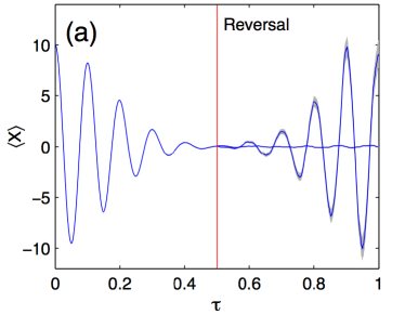
Figure 5: Time-reversal test of anharmonic oscillator with $N=100$ initial bosons in a coherent state. The shaded areas for $\tau>0.5$ indicate a slowly growing sampling error-bar, calculated using the central limit theorem and the sampled variance.

This calculation also demonstrates a subtle feature of the +P stochastic method, which is that the phase-space distribution is not unique! In fact, a moment’s thought serves to illustrate that this is a necessary feature of a stochastic method that represents unitary evolution in quantum mechanics. If the mapping has stochastic behavior during the time-evolution, then it will spread in the phase-space as time evolves. Technically, the phase-space entropy must increase.

Yet reversing time simply results in another type of unitary evolution, also with a stochastic equivalent. The result is that the phase-space distribution spreads even more, increasing the phase-space entropy yet further. This is illustrated in Fig (6), which graphs the distribution underlying the mean quadratures depicted in Fig (5). Clearly, the final distribution after time-reversal is totally different from the initial distribution, which is a delta-function in phase-space. The final distribution after time-reversal is a Gaussian convolution of the original delta-function. Despite this, the two distributions are physically identical, and have identical observable moments due to the non-uniqueness of the basis set.

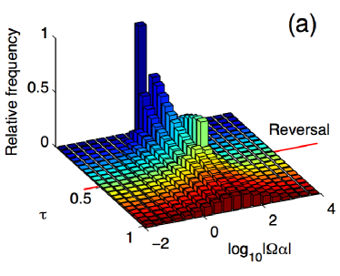
Figure 6: Phase-space distributions, showing non-uniqueness after time-reversal at normalized time $\tau=0.5$. The horizontal axis is a product of the phase-space coordinate $\alpha$ and the random stochastic weight $\Omega$.

V.5 BEC collision: $10^{5}$ bosons, $10^{6}$ spatial modes

Next we consider a case of extremely large complexity: a collision of two Bose condensates, each with a very large number of particles and modes.

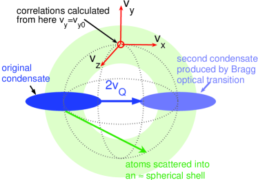
Figure 7: Schematic diagram of a BEC collision. A second condensate is produced in situ by a Bragg scattering pulse, with a relative velocity of $2v_{Q}$, causing a quantum collision. This results in quantum correlated atoms scattering into a spherical shell of velocities around the original mean velocity.

Recent experiments on ultra-cold Bose-Einstein condensates have been able to generate collisions of quantum condensates with large numbers ($>10^{5}$) of particlesprl-89-020401 . These experiments typically use metastable ${}^{4}He^{*}$ condensates so that he particle correlations can be readily measured. The initial state is simply a trapped BEC in which half the atoms have been accelerated to a high relative velocity compared to the other half using optical Bragg scattering techniques, as shown in Fig (7). Atoms collide to produce a scattered halo of correlated atoms, involving both spontaneous and stimulated emission into the scattered modes. These quantitative experiments provide a rigorous test of the methodology of these simulations.

We consider the collisiondeuar_drummond_07 of two pure ²³Na BECs, with a similar design to a recent experiment at MITvogels_xu_02 , and more recent experiments in Francekrachmalnicoff_jaskula_10 . A $1.5\times 10^{5}$ atom condensate is prepared in a cigar-shaped magnetic trap with frequencies 20 Hz axially and 80 Hz radially. A brief Bragg laser pulse is used to coherently impart a velocity of ${2{\rm v_{Q}}}=19.64$ mm/s to half of the atoms, that is much greater than the sound velocity of $3.1$ mm/s. At this point the trap is turned off so that the wavepackets collide freely.

The coupling constant $g$ depends on the s-wave scattering length $a$ ($2.75$nm in the case of ²³Na). We begin the simulation in the center-of-mass frame at the moment the lasers and trap are turned off ($t=0$). The initial wavefunction is modeled as the coherent-state mean-field Gross-Pitaevskii (GP) solution of the trapped $t<0$ condensate, but modulated with a factor $\left[e^{ik_{{\rm Q}}{\rm x}}+e^{-ik_{{\rm Q}}{\rm x}}\right]/\sqrt{2}$ which imparts initial velocities ${\rm v_{x}}={\rm\pm v_{Q}}=\pm\hbar k_{{\rm Q}}/m$ in the ${\rm x}$ direction.

Collisions have been calculated for up to $10^{6}$ modes and $10^{5}$ interacting bosonsprl-98-120402 . This is a clearly exponential regime, yet the +P technique is definitely applicable. There are restrictions on the interaction density and total time duration possible before the sampling error is too large, but useful results are certainly obtainable, as shown in Fig (8). We emphasize that sampling error, while easily estimated, is not easily reduced at long times due to a rapid growth in the distribution variance, which eventually makes these simulations impractical.

By comparison, with the same parameters the truncated Wigner method clearly fails to produce physically sensible results. There is an uncontrolled error leading to a completely unphysical depletion of the vacuum at large relative velocity, causing apparently negative particle densities which of course cannot occur. This depletion leads to ‘ghost’ particles scattering into low-velocity regions near the original condensate velocity, which do not correspond to any real physical events.

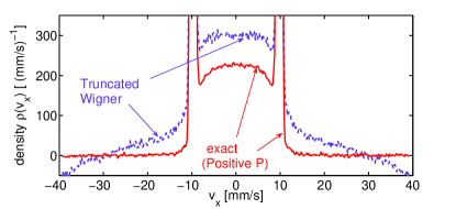
Figure 8: Comparison of truncated Wigner and +P simulations, for total scattered particle density in velocity space at a given final velocity. While the +P results agree with experiments, the results show unphysical negative densities and ‘ghost’ scattering events in the approximate truncated Wigner approach. In these simulations, space is discretized onto a $432\times 50\times 50$ lattice with $k_{{\rm x,max}}=1.4\times 10^{7}$/m and $k_{{\rm y,z,max}}=6.2\times 10^{6}$/m, giving $10^{6}$ modes in total, with physical parameters given in the text.

While the +P simulation produces physically sensible results up to the time when sampling errors are too large to be useful, the truncated Wigner approach is liable to generate completely unphysical behavior. This is due to the fact that in a three-dimensional quantum field simulation, there are a diverging number of unoccupied high-momentum modes in the limit of high momentum cutoff. These contradict the basic high-occupation number approximation inherent in the Wigner truncation.

In summary, the advantages and disadvantages of the +P approach are that it treats exponentially large Hilbert spaces without mean-field or factorization assumptions, including either unitary or non-unitary damped evolution. No truncation of the equations of motion is required , and there is no UV divergence at large k-value. However, for unitary evolution, and especially for strong interactions, the sampling error grows in time. This is intrinsic to the stochastic method, which leads to solutions have relatively large tails. From the fundamental existence theorem, there are known solutions that are strongly bounded with small sampling errors, but one must use different simulation techniques to access these solutions.

VI Gaussian Representation

The Gaussian phase-representation is a more general phase-space representation than either the Wigner or positive-P method. In fact, it includes these as special cases, and extends the phase-space idea to include fermions Corney:2003 ; corney_drummond_06c . Here we consider a general number-conserving Gaussian operator basis, in which any density matrix ${\rho}$ is expanded in terms of Gaussian operators, ${\Lambda}(\bm{\lambda})$, defined as exponentials of quadratic forms. In order to define the Gaussian operators, we consider a bosonic or fermionic quantum field with an $M$-dimensional set of mode operators ${\bm{a}}^{\dagger}\equiv\left[{a}_{1}^{\dagger},{a}_{2}^{\dagger},\ldots{a}_{M}^{\dagger}\right]$. In the bosonic case, we can define $\delta{\bm{a}}={\bm{a}}-\bm{\alpha}$ and $\delta{\bm{a}}^{\dagger}={\bm{a}}^{\dagger}-\bm{\beta}$ as operator displacements, where in general $\bm{\alpha}$ and $\bm{\beta}^{\dagger}$ are independent complex vectors. In the fermionic case we set these displacements to zero. The annihilation and creation operators satisfy (anti) commutation relations, with ($+$) for fermions and ($-$) for bosons:

$$\left[{a}_{i,}{a}_{j}^{\dagger}\right]_{\pm}=\delta_{ij}.$$ (46)

The expansion of the density matrix is:

$${\rho}=\int P(\bm{\lambda}){\Lambda}(\bm{\lambda})d\bm{\lambda}\,\,,$$ (47)

where $P(\bm{\lambda})$ is the probability density over the phase-space, $\bm{\lambda}$ is the complex vector parameter of the Gaussian representation , $d\bm{\lambda}$ is the integration measure, and ${\Lambda}(\bm{\lambda})$ is a Gaussian operator, defined as a normally ordered exponential of a quadratic form of annihilation and creation operators:

$${\Lambda}(\bm{\lambda})=\frac{1}{{\cal N}}{\Lambda}_{u}\left(\bm{\lambda}\right)=\frac{1}{{\cal N}}:\exp\left[-\delta{\bm{a}}^{\dagger}\underline{\bm{\mu}}\delta{\bm{a}}\right]:$$ (48)

Here, $\underline{\bm{\mu}}$ is a complex $M\times M$ matrix, so that the representation phase space is $\bm{\lambda}=\left[\bm{\alpha},\bm{\beta},\underline{\bm{\mu}}\right]$. ${\cal N}=Tr\left[{\Lambda}_{u}(\bm{\lambda})\right]$ is a normalizing factor, and $:\,:$ indicates normal ordering. The normalizing factor has two forms, for bosons and fermions respectively:

$${\cal N}_{b} = \det\left[\underline{\bm{\mu}}\right]^{-1}$$

$${\cal N}_{f} = \det\left[2\underline{\bm{I}}-\underline{\bm{\mu}}\right]\,.$$ (49)

The matrix $\underline{\bm{\mu}}$ is related to the stochastic Green’s function $\underline{\bm{n}}$ as:

$$\underline{\bm{n}}_{b} = \underline{\bm{\mu}}^{-T}-\underline{\bm{I}}$$

$$\underline{\bm{n}}_{f} = \left[2\underline{\bm{I}}-\underline{\bm{\mu}}\right]^{-T}\,.$$ (50)

In either case, the stochastic average of $\underline{\bm{n}}$ over the distribution $P$ is physically a normally ordered many-body Green’s function, so that:

$$\left\langle{a}_{i}^{\dagger}{a}_{j}\right\rangle=\left\langle n_{ij}+\beta_{i}\alpha_{j}\right\rangle_{P}\,.$$ (51)

Similar methods to the positive-P approach can then be used for calculating time-evolution. These have been used very successfully in treating, for example, the ground state of the fermionic Hubbard model aimi_imada_07 - a problem of much interest in condensed matter physics.

VI.1 Linear entropy

Entropy is a measure of loss of information and entanglement in a quantum system, and it is important to have a method of sampling a phase-space distribution in order to estimate the entropy. Here we show that the Gaussian phase-space method is well-suited to this type of calculation. In particular, the linear or Renyi entropyRenyi_1960 , is defined as:

$$S_{2}=-\ln Tr\left({\rho}^{2}\right)\,\,.$$ (52)

This has similar properties to the usual logarithmic entropy, and measures state purity, since $S_{2}=0$ for a pure state, while $S_{2}>0$ for a mixed state. The Renyi entropy in a phase-space representation can be written using Eq. (52) and the expansion of the density matrix Eq. (47) as:

$$S_{2}=-\ln\iint P(\bm{\lambda})P(\bm{\lambda}^{\prime})Tr\left({\Lambda}(\bm{\lambda}){\Lambda}(\bm{\lambda}^{\prime})\right)\,d\bm{\lambda}d\bm{\lambda}^{\prime}\,.$$ (53)

In order to obtain an expression of the linear entropy using the Gaussian phase-representation is necessary to evaluate the inner products of Gaussian operators of form $Tr\left({\Lambda}(\bm{\lambda}){\Lambda}(\bm{\lambda}^{\prime})\right)$ZaratePhysRevA2011 . We emphasize here that this procedure does not give useful results for the usual classical phase-space representations. However, we will show that it yields remarkably simple results for both fermionic and bosonic Gaussian representations.

For the fermionic case, we first evaluate the trace of the inner product of two un-normalized fermionic operators $F\left(\underline{\bm{\mu}},\underline{\bm{\nu}}\right)=Tr\left[{\Lambda}_{u}\left(\underline{\bm{\mu}}\right){\Lambda}_{u}\left(\underline{\bm{\nu}}\right)\right]$. In this approach, the physical many-body system is treated as a distribution over fermionic Green’s functions, whose average are the observed Green’s function or correlation function.

In order to evaluate the trace we use fermionic coherent states $|\bm{\alpha}\rangle$ in terms of Grassmann variables $\bm{\alpha}$Cahill1999a , as well as the trace of an operator and the identity operator of fermionic coherent states. After some Grassmann calculus, we obtain that the inner product of two un-normalized fermionic Gaussian operators is:

$$F\left(\underline{\bm{\mu}},\underline{\bm{\nu}}\right)=\det\left[\bm{\mathrm{I}}\,+\left(\underline{\bm{I}}-\underline{\bm{\mu}}\right)\left(\underline{\bm{I}}-\underline{\bm{\nu}}\right)\right].$$ (54)

We rewrite these expressions in terms of the normally ordered Green’s functions or correlations of the basis sets:

$$n_{ij}=Tr\left[{\Lambda}(\mathbf{n}){a}_{i}^{\dagger}{a}_{j}\right].$$ (55)

Introducing the hole Green’s functions, $\tilde{\underline{\mathbf{n}}}=\left[\underline{\bm{\mathrm{I}}}-\underline{\mathbf{n}}\right]$, and $\tilde{\underline{\mathbf{m}}}=\left[\underline{\bm{\mathrm{I}}}-\underline{\mathbf{m}}\right]$, we obtain the following result for the normalized inner product of fermionic Gaussian operators:

$$Tr\left[{\Lambda}(\mathbf{m}){\Lambda}(\mathbf{n})\right]=\det\left[\tilde{\underline{\mathbf{n}}}\tilde{\underline{\mathbf{m}}}+\underline{\mathbf{n}}\underline{\mathbf{m}}\right].$$ (56)

Using the result of the trace of the inner product of fermionic Gaussian operators, Eq.  (56), we obtain that the expression for the linear entropy in a Gaussian phase representation Eq.  (53) is:

$$S_{2}=-\ln\iint P(\bm{m})P(\bm{n})\det\left[\tilde{\underline{\mathbf{n}}}\tilde{\underline{\mathbf{m}}}+\underline{\mathbf{n}}\underline{\mathbf{m}}\right]\,d\mathbf{m}d\mathbf{n}\,.$$ (57)

Just as in the case of fermions, we evaluate the inner product of two un-normalized bosonic Gaussian operators, $B\left(\underline{\bm{\mu}},\underline{\bm{\nu}}\right)=Tr\left[{\Lambda}_{u}\left(\underline{\bm{\mu}}\right){\Lambda}_{u}\left(\underline{\bm{\nu}}\right)\right]$ , and after using coherent state expansions, we obtain that the inner product of two un-normalized bosonic Gaussian operators is:

$$B\left(\underline{\bm{\mu}},\underline{\bm{\nu}}\right)=\det\left[\bm{\mathrm{I}}\,-\left(\underline{\bm{\mu}}-\underline{\bm{I}}\right)\left(\underline{\bm{\nu}}-\underline{\bm{I}}\right)\right]^{-1}$$ (58)

Similar to the fermionic case, we can rewrite this expression in terms of the stochastic Green’s functions, and finally we have that:

$$S_{2}=\ln\iint P(\bm{m})P(\bm{n})\det\left[\underline{\bm{\mathrm{I}}}+\underline{\mathbf{n}}+\underline{\mathbf{m}}\right]\,d\mathbf{m}d\mathbf{n}\,.$$ (59)

In summary, using the results of the inner products of Gaussian operators, we can obtain an expression for the linear entropy. Since this is just an average over two independent probabilities, it is readily calculable using sampled phase-space representations. This expression can also be used to evaluate the entanglement of a quantum system with a reservoir or other coupled system.

VII Variational methods

While the previous phase-space methods have had a long history in physics, there is a different approach with an equally long history, namely the use of variational techniques. This is a very simple concept, which is that one should use an evolution equation which minimizes the error.

The idea was first proposed by Frenkel(Frenkel-Wave, , p436) and Dirac, who developed early variational methods. In Dirac’s original approach, an effective action method was proposed for a variational wave-function $\left|\psi\left(t\right)\right\rangle$, of the form:

$$\delta\Gamma=\delta\int dt\left\langle\psi\left(t\right)\right|\left[i\hbar\partial_{t}-{H}\right]\left|\psi\left(t\right)\right\rangle=0$$ (60)

This generates a variational Schroedinger equation, which gives the exact Schroedinger equation in the case that $\left|\psi\left(t\right)\right\rangle$ is a complete set of wave-functions. In the usual application of the method, $\left|\psi\left(t\right)\right\rangle$ is chosen as a specific functional form described by a small number of free parameters. The properties of this method are that results depend on the chosen function, and there are a small number of equations. However, one can’t easily determine errors, and of course, the method doesn’t converge if $\left|\psi\left(t\right)\right\rangle$ is incomplete.

VII.1 Multiconfigurational methods

More recent applications of the variational approachMeyer-Multidimensional have focused on the concept of choosing an expansion for the variational wavefunction that is complete in some limit. These are typically sums of individual many-body wavefunctions known as configurations, hence the term multi-configurational approach. A common approach in the BEC case is to construct the variational wavefunction from sums of multiply-occupied Fock states of the formpra-77-33613 :

$$\left|\psi\left(t\right)\right\rangle\ldots=\sum_{\vec{n}}C_{\vec{n}}\left(t\right){a}_{1}^{n_{1}}\ldots{a}_{M}^{n_{M}}\left|0\right\rangle\,,$$ (61)

where the operators ${a}_{j}^{\dagger}$ are time-dependent operators such that:

$${a}_{j}^{\dagger}=\int d^{3}\mathbf{r}{\Psi}^{\dagger}\left(\mathbf{r}\right)\phi_{j}\left(\mathbf{r},t\right)\,.$$ (62)

Compared to the usual variational approach, the strategy used here is to systematically increase the Hilbert space dimension by increasing the number of modes, with full convergence expected as $M\rightarrow\infty$ . An obvious drawback is that, since $M$ is the number of modes, and the Hilbert space is essentially a standard Fock space, there is clearly a potential problem with this strategy. There is an exponential complex Hilbert space dimension as $\,M$ increases. The result of this problem is that the technique is currently restricted to one dimension with less than 100 particles, and relatively weak interactions. However, given this restriction, relatively long interaction times are possible.

VII.2 Combining phase-space and variational methods

Given the success of phase-space approach in dealing with complexity, an obvious question is: how can we unify variational and coherent states phase-space methods? Such an approach would have several potential advantages. Coherent states provide description of long-range coherence, and in principle are a complete basis. The usual stochastic method with finite computational samples can cause a large sampling error. However, the variational approach can be used to minimize the error. The goal of such an approach is to combine a high degree of complexity with relatively long time-scale evolution.

In order to describe the simplest resulting method of this type, we recall the Wheeler-Everett multiverse conceptrmp-29-454 . That is, suppose we let $\left|\bm{\alpha}\right\rangle$ be a multi-mode coherent state, then an $\mathcal{N}$ component superposition of coherent states can be considered a ‘multiverse’ - a superposition of $\mathcal{N}$ classical worlds. This is parameterized by a coherent ‘super-vector $\,\mathbf{X}\equiv\left(\bm{\alpha}^{(1)},\ldots\bm{\alpha}^{(\mathcal{N})}\right)$, where $\bm{\alpha}=\left(\alpha_{0},\ldots\alpha_{M}\right)$ is a multi-mode coherent amplitude, ${a}_{0}\equiv{1}$ is the unit operator, and $\alpha_{0}$ is introduced here as a combined relative phase and weight parameter, including the state normalization factor. The corresponding quantum state defined as:

$$\left|\psi\left(t\right)\right\rangle =\,\sum_{n=1}^{\mathcal{N}}e^{\bm{\alpha}^{(n)}\left(t\right)\cdot{\mathbf{a}}^{\dagger}}\left|0\right\rangle$$ (63)

This is a constrained multiverse, with a fixed number of copies, shown schematically in Fig (9). One cannot keep track of all quantum universes! It is also, in quantum mechanical terms, a superposition of non-orthogonal coherent states. We find that the use of a variational principle introduces interactions between coherent amplitudes. The advantage is a much lower sampling error compared to independent stochastic evolution.

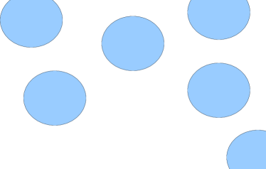
Figure 9: What does the multiverse look like? Here we give an illustration of a quantum ‘universe’ as a superposition of coherent states, illustrated by the blue circles. Each blue circle represents a different multi-mode coherent state $\bm{\alpha}^{(n)}\left(t\right)$, which has an intrinsic uncertainty. The whole quantum state or ‘universe’ is a superposition of $\mathcal{N}$ coherent states with different phases and amplitudes.

VII.3 Phase-space variational equations

Having introduced the concept, we now wish to derive the resulting equationsjcp-128-044116 . Suppose the Hamiltonian is $\,H\left({\mathbf{a}}^{\dagger},{\mathbf{a}}\right)$, with an exact wavefunction $\left|\tilde{\psi}\right\rangle$, and a time-interval $\Delta t=t-t_{0}$, then clearly:

$$\,\left|\tilde{\psi}\left(t\right)\right\rangle=e^{-i{H}\Delta t}\left|\psi\left(t_{0}\right)\right\rangle\,\,.$$ (64)

We wish to minimize local propagation error in calculating the computational result$\left|\psi\left(t\right)\right\rangle$, so that:

$$\delta\mathcal{E}=\,\delta\left\|\left|\psi\left(t\right)\right\rangle-e^{-i{H}\Delta t}\left|\psi\left(t_{0}\right)\right\rangle\right\|^{2}=0.$$ (65)

Expanding to first order and taking the limit of $\Delta t=t-t_{0}\rightarrow 0$, gives:

$$\Re\left\langle\delta\psi\right|\left[\partial_{t}+i{H}\right]\left|\psi\right\rangle=0\,.$$ (66)

We introduce $\left|\Delta\psi\right\rangle=\left|\psi\left(t\right)\right\rangle-\left|\psi\left(t_{0}\right)\right\rangle$ and linearize in the coherent state parameters, so that:

$$\left|\Delta\psi\right\rangle=\Delta X_{\mu}\frac{\partial\left|\psi\right\rangle}{\partial X_{\mu}}$$ (67)

The variational principle then leads to a differential equation for the coherent parameters $\mathbf{X}$, of form:

$$\,\partial_{t}\mathbf{X}=-i\mathcal{\boldsymbol{V}}^{-1}\mathcal{\mathcal{\mathbf{H}}}\,.$$ (68)

This means that there are now $P\equiv\mathcal{N}(M+1)$ differential equations to solve, with a combined index $\mu,$ where the main terms are

• The variational matrix: $\,\mathcal{V}_{\mu\nu}=\left\{\frac{\partial}{\partial X_{\mu}}\left\langle\psi\right|\right\}\,\frac{\partial}{\partial X_{\nu}}\left|\psi\right\rangle$

• The H-vector: $\,\mathcal{H}_{\mu}=\left\{\frac{\partial}{\partial X_{\mu}}\left\langle\psi\right|\right\}\,{H}\left|\psi\left(t\right)\right\rangle.$

However, a numerical problem must be treated, which is that $\mathcal{V}_{\mu\nu}$ is generally not invertible, owing to the existence of multiple minima. We can solve this iteratively, in terms of the parameter change $\Delta\mathbf{X}^{[p]}$, where we set $\Delta\mathbf{X}^{[0]}=0$ initially and iterate until a stable solution is reached. This is similar to the Tikhonov variational methodTikhonov-Nonlinear . In detail, suppose we have a set of variational parameters $\mathbf{X}\left(t_{0}\right)$, at time $t=t_{0}$. We evaluate the variational matrix and Hamiltonian vector a midpoint $t_{0}+\Delta t/2$, by iterating so that $\mathbf{X}^{[p-1]}=\mathbf{X}\left(t_{0}\right)+\Delta\mathbf{X}^{[p-1]}$, and setting the change in $\mathbf{X}$ to $\Delta\mathbf{X}^{[p]}$, where:

$$\Delta\mathbf{X}^{[p]} =\Delta\mathbf{X}^{[p-1]}+\left[\mathcal{\mathbf{\mathcal{V}}}^{[p-1]}+i\lambda\mathbf{I}\right]^{-1}\times$$

$$\times\left[-i\Delta t\mathcal{H}^{[p-1]}/2-\mathcal{\mathbf{\mathcal{V}}}^{[p-1]}\Delta\mathbf{X}^{[p-1]}\right]$$ (69)

The final step is to propagate to $t_{0}+\Delta t$ by setting:

$$\mathbf{X}\left(t_{0}+\Delta t\right)=\mathbf{X}\left(t_{0}\right)+2\Delta\mathbf{X}^{[p]}\,,$$ (70)

in order to move to the next step in time. This method leads to stable equations, with no inversion problems.

In the case of a coherent state expansion, we define an energy matrix:

$$H^{(m,n)}=H\left(\bm{\alpha}^{(m)*},\bm{\alpha}^{(n)}\right)\,,$$ (71)

a reduced amplitude:

$$\,\tilde{\alpha}_{k}^{(m)}=\delta_{k0}+\left[1-\delta_{k0}\right]\alpha_{k}^{(m)},\,$$ (72)

and an inner product:

$$\,\rho^{(mn)}=\exp\left[\alpha_{0}^{(m)*}+\alpha_{0}^{(m)}+\sum_{k>0}\alpha_{k}^{(m)*}\alpha_{k}^{(n)}\right]\,.$$ (73)

The variational matrix definitions are then:

$$V_{kl}^{(mn)} \,=\,\left[\left[1-\delta_{k0}\right]\delta_{kl}+\tilde{\alpha}_{l}^{(m)*}\tilde{\alpha}_{k}^{(n)}\right]\rho^{(mn)}$$

$$H_{k}^{(m)} \,=\,\sum_{n}\left[\frac{\partial H^{(m,n)}}{\partial\alpha_{k}^{(m)*}}+H^{(m,n)}\tilde{\alpha}_{k}^{(n)}\right]\rho^{(mn)}\,\,.$$ (74)

For example, in the case of a single variational term, one finds equations equivalent to the Gross-Pitaevskii mean-field equation, with an additional phase evolution for $\alpha_{0}$:

$$\,\partial_{t}\alpha_{0} \,= \,-i\left[H-\bm{\alpha}^{\dagger}\cdot\partial H/\partial\bm{\alpha}^{\dagger}\right]$$

$$\,\partial_{t}\bm{\alpha} \,= \,-i\partial H/\partial\bm{\alpha}^{\dagger}\,\,.$$ (75)

For a linear Hamiltonian:

$$\,{H}={\mathbf{a}}^{\dagger}\bm{\omega}{\mathbf{a}}\,$$ (76)

one finds that each coherent term evolves independently of each other term, giving:

$$\,\partial_{t}\alpha_{0}^{(n)} \,= \,0$$

$$\,\partial_{t}\bm{\alpha}^{(n)} \,= \,-i\bm{\omega}\bm{\alpha}^{(n)}\,\,.$$ (77)

In this case each linear ‘universe’ is decoupled from the others; this is an exact result, and no approximations are required.

VII.4 Recurrences in the anharmonic oscillator

Finally, we consider the case of a quantum anharmonic oscillator, which describes local S-wave scattering interactions at a single lattice site, so that:

$$\,{H}={a}^{\dagger 2}{a}^{2}$$ (78)

This is an extremely strong test of coherent state expansion methods. From an initial coherent state the quantum evolution generates Schroedinger cat superpositions, with complete recurrences known to occur analyticallypra-33-674 , as well as experimentally Greiner_02 . Variational results showing almost error-free dynamics throughout the Schroedinger-cat regime of $t=\pi$, and a complete recurrence at $t=2\pi$ are shown in the figures. For these numerical results, we used $\lambda=10^{-4}$ to control the matrix inversion, with four iterations of the variational equations at each time point.

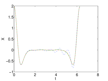
Figure 10: Anharmonic recurrence, x quadrature. Blue dashed line has $8$ components, green solid line has $16$ components. This is almost indistinguishable from the the exact solution, which is a red dashed line.

Here we define quadrature variables,

$$X=\left\langle{a}+{a}^{\dagger}\right\rangle/2$$ (79)

and

$$Y=\left\langle{a}-{a}^{\dagger}\right\rangle/(2i\mbox{})$$ (80)

The exact result, given an initial coherent state, is known to have recurrences in both quadratures, as shown in the graphs.

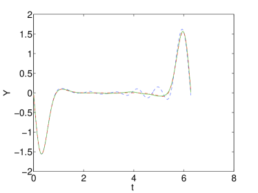
Figure 11: Anharmonic recurrence, y quadrature. Parameters as in the previous figure. The blue dashed line with small oscillations is not quite converged, while the solid green line shows excellent convergence to the exact result.

While it is simple enough to be analytically soluble, this Hamiltonian would lead to large errors with stochastic phase-space techniques over time-scales comparable to the recurrence time. As we show in Figs (10) and (11), the use of a variational method allows us to track the full recurrence, on timescales where any previous stochastic phase-space method would give very large errors Deuar:2002 ; deuar_drummond_06 ; dowling_drummond_05 . Variational convergence is rapid, with only small errors visible using $\mathcal{N}=8$ components. These are almost completely eliminated by using $\mathcal{N}=16$ coherent components. This illustrative example is very simple, and indeed the case treated here can be solved exactly using analytic techniques. However, it does illustrate the utility of variational methods in reducing sampling error in phase-space simulations.

VIII Outlook and summary

In summary, there are a growing number of experiments in ultra-cold atomic physics that probe the world of quantum dynamics. Simple, exact results are only possible with a small number of interacting modes. Larger, complex quantum systems require new techniques to handle the issue of exponential complexity. While phase-space representations using non-orthogonal basis sets can can treat highly complex problems, there is often a problem with truncations (in the Wigner case) or sampling errors that grow in time (in the positive-P case).

We have shown that there are newer techniques that have much promise. Gaussian phase-space methods are much more general, and can treat new issues like fermions and entropy calculations. Finally, we have derived a Tikhonov-based variational approach which is shown to dramatically reduce sampling errors in a case which is known to be challenging to handle with phase-space methods. This approach gives exact results for linear couplings. It has lower sampling errors than the stochastic +P method, as well as reduced variational complexity issues compared to multi-configurational approaches in a Fock space basis. While the techniques given here are only preliminary, this hybrid variational and phase-space approach appears promising for future developments.

References

- (1) D. Heinzen, R. Wynar, P. D. Drummond, and K. V. Kheruntsyan, Physical Review Letters 84, 5029 (May 2000), ISSN 0031-9007, http://link.aps.org/doi/10.1103/PhysRevLett.84.5029
- (2) E. A. Donley, N. R. Claussen, S. T. Thompson, and C. E. Wieman, Nature 417, 529 (May 2002), ISSN 0028-0836, http://www.ncbi.nlm.nih.gov/pubmed/12037562
- (3) A. E. Leanhardt, T. A. Pasquini, M. Saba, A. Schirotzek, Y. Shin, D. Kielpinski, D. E. Pritchard, and W. Ketterle, Science (New York, N.Y.) 301, 1513 (Sep. 2003), ISSN 1095-9203, http://www.sciencemag.org/content/301/5639/1513.abstract
- (4) S. Datta, Electronic Transport in Mesoscopic Systems (Cambridge University Press, Cambridge, 1995) ISBN 0521599431, http://www.amazon.com/Electronic-Mesoscopic-Semiconductor-Microelectron%ic-Engineering/dp/0521599431/
-
(5)
H. J. Metcalf and P. van der Straten, Laser Cooling and Trapping (Springer, 1999) ISBN 0387987282, p. 339, http://www.amazon.com/Cooling-Trapping-Graduate-Contemporary-Physics/dp%/0387987282.
Key: Metcalf-Laser
Annotation: Bose-Einstein condensate textbook. - (6) M. Schellekens, R. Hoppeler, A. Perrin, J. V. Gomes, D. Boiron, A. Aspect, and C. I. Westbrook, Science (New York, N.Y.) 310, 648 (Oct. 2005), ISSN 1095-9203, http://www.sciencemag.org/content/310/5748/648.abstract
- (7) A. Robert, O. Sirjean, A. Browaeys, J. Poupard, S. Nowak, D. Boiron, C. I. Westbrook, and A. Aspect, Science (New York, N.Y.) 292, 461 (Apr. 2001), ISSN 0036-8075, http://www.sciencemag.org/content/292/5516/461.abstract
- (8) J. M. Vogels, K. Xu, and W. Ketterle, Physical Review Letters 89, 020401 (Mar. 2002), arXiv:0203286 [cond-mat], http://arxiv.org/abs/cond-mat/0203286
-
(9)
F. A. Berezin, The Method of Second Quantization (Academic Press, New York, 1966) ISBN 0120894505, http://www.amazon.com/Method-Second-Quantization-F-Berezin/dp/012089450%5.
Key: Berezin-Method
Annotation: Available in U Melbourne physics library, 530.12 B492 Translated from the Russian. How does one cite it? - (10) P. D. Drummond and S. J. Carter, J. Opt. Soc. Am. B 4, 1565 (1987)
- (11) D.-I. Choi and Q. Niu, Physical Review Letters 82, 2022 (Mar. 1999), ISSN 0031-9007, http://link.aps.org/doi/10.1103/PhysRevLett.82.2022
- (12) J. H. Denschlag, J. E. Simsarian, H. Haeffner, C. McKenzie, A. Browaeys, D. Cho, K. Helmerson, S. L. Rolston, and W. D. Phillips, Journal of Physics B: Atomic, Molecular and Optical Physics 35, 3095 (Jun. 2002), ISSN 09534075, arXiv:0206063 [cond-mat], http://stacks.iop.org/0953-4075/35/i=14/a=307?key=crossref.143851fbd4f7%95110e47d745ef41278chttp://arxiv.org/abs/cond-mat/0206063
-
(13)
J. Hubbard, Proceedings of the Royal
Society A: Mathematical, Physical and Engineering Sciences 276, 238 (Nov. 1963), ISSN 1364-5021, http://rspa.royalsocietypublishing.org/cgi/doi/10.1098/rspa.1963.0204.
Key: rsa-276-238
Annotation: Swinburne doesn’t have it! - (14) R. P. Feynman, International Journal of Theoretical Physics 21, 467 (Jun. 1982), ISSN 0020-7748, http://www.springerlink.com/index/10.1007/BF02650179http://www.phy.mtu.edu/~sgowtham/PH4390/Week_02/IJTP_v21_p467_y1982.pdf
- (15) Q. Y. He, M. D. Reid, T. G. Vaughan, C. Gross, M. Oberthaler, and P. D. Drummond, Phys. Rev. Lett. 106 (2011)
- (16) T. J. Haigh, A. J. Ferris, and M. K. Olsen, Optics Communications 283, 3540 (2010)
- (17) P. D. Drummond, R. M. Shelby, S. R. Friberg, and Y. Yamamoto, Nature 365, 307 (1993)
- (18) V. Giovannetti, S. Mancini, D. Vitali, and P. Tombesi, Phys. Rev. A 67, 022320 (2003)
- (19) R. Dong, J. Heersink, J.-I. Yoshikawa, O. Glockl, U. L. Andersen, and G. Leuchs, New J. Phys. 9, 410 (2007)
- (20) W. P. Bowen, N. Treps, R. Schnabel, and P. K. Lam, Phys. Rev. Lett. 89, 253601 (2002)
- (21) C. W. Gardiner and P. Zoller, Quantum Noise, 2nd ed. (Springer-Verlag, Berlin, 2000) ISBN 3-540-66571-4
- (22) E. P. Wigner, Phys. Rev. 40, 749 (1932)
- (23) R. J. Glauber, Phys. Rev. 131, 2766 (1963)
- (24) E. C. G. Sudarshan, Phys. Rev. Lett. 10, 277 (1963)
- (25) K. Husimi, Proc. Phys. Math. Soc. Jpn 22, 264 (1940)
- (26) S. J. Carter, P. D. Drummond, M. D. Reid, and R. M. Shelby, Phys. Rev. Lett. 58, 1841 (1987)
- (27) S. J. Carter and P. D. Drummond, Phys. Rev. Lett. 67, 3757 (1991)
- (28) P. D. Drummond and A. D. Hardman, EuroPhys. Lett. 21, 279 (1993)
- (29) P. D. Drummond, R. M. Shelby, S. R. Friberg, and Y. Yamamoto, Nature 365, 307 (1993)
- (30) P. D. Drummond and J. F. Corney, J. Opt. Soc. Am. B 18, 139 (2001)
- (31) M. Rosenbluh and R. M. Shelby, Phys. Rev. Lett. 66, 153 (1991)
- (32) J. Heersink, V. Josse, G. Leuchs, and U. L. Andersen, Opt. Lett. 30, 1192 (2005)
- (33) J. F. Corney, P. D. Drummond, J. Heersink, V. Josse, G. Leuchs, and U. L. Andersen, Phys. Rev. Lett. 97, 023606 (2006)
- (34) M. J. Steel, M. K. Olsen, L. I. Plimak, P. D. Drummond, S. M. Tan, M. J. Collet, D. F. Walls, and R. Graham, Physical Review A 58, 4824 (1998)
- (35) P. B. Blakie, A. S. Bradley, M. J. Davis, R. J. Ballagh, and C. W. Gardiner, Advances in Physics 57, 363 (2008)
- (36) M. Egorov, R. P. Anderson, V. Ivannikov, B. Opanchuk, P. Drummond, B. V. Hall, and A. I. Sidorov, Phys. Rev. A 84 (AUG 22 2011), ISSN 1050-2947
- (37) R. Glauber, Physical Review 131, 2766 (Sep. 1963), ISSN 0031-899X, http://link.aps.org/doi/10.1103/PhysRev.131.2766
- (38) K. Cahill and R. Glauber, Physical Review A 59, 1538 (Feb. 1999), ISSN 1050-2947, http://link.aps.org/doi/10.1103/PhysRevA.59.1538
- (39) J. F. Corney and P. D. Drummond, Physical Review A 68, 23 (Aug. 2003), ISSN 1050-2947, arXiv:0308064 [quant-ph], http://link.aps.org/doi/10.1103/PhysRevA.68.063822http://arxiv.org/abs/quant-ph/0308064
- (40) K. E. Cahill and R. J. Glauber, Phys. Rev. 177, 1857 (1969)
- (41) J. E. Moyal, Math.l Proc. Camb. Phil. Soc. 45, 99 (1949)
- (42) P. D. Drummond and A. D. Hardman, Europhysics Letters 21, 279 (jan 1993), ISSN 0295-5075, http://stacks.iop.org/0295-5075/21/i=3/a=005?key=crossref.5ced39e5bf433%e75a804fe992a5bc20e
- (43) M. Steel, M. K. Olsen, L. I. Plimak, P. D. Drummond, S. Tan, M. J. Collett, D. Walls, and R. Graham, Physical Review A 58, 4824 (dec 1998), ISSN 1050-2947, http://link.aps.org/doi/10.1103/PhysRevA.58.4824
- (44) A. Sinatra, C. Lobo, and Y. Castin, Journal of Physics B 35, 3599 (sep 2002), ISSN 0953-4075, http://stacks.iop.org/0953-4075/35/i=17/a=301?key=crossref.c7aed7eb9dc5%ce0bb952f7815936c80e
- (45) M. W. Jack, Physical Review Letters 89, 140402 (sep 2002), ISSN 0031-9007, http://link.aps.org/doi/10.1103/PhysRevLett.89.140402
- (46) A. Sørensen, L. M. Duan, J. I. Cirac, and P. Zoller, Nature 409, 63 (jan 2001), ISSN 0028-0836, http://www.ncbi.nlm.nih.gov/pubmed/11343111
- (47) D. J. Wineland, J. Bollinger, W. Itano, and D. Heinzen, Physical Review A 50, 67 (jul 1994), ISSN 1050-2947, http://link.aps.org/doi/10.1103/PhysRevA.50.67
- (48) A. Kaufman, R. P. Anderson, T. Hanna, E. Tiesinga, P. Julienne, and D. Hall, Physical Review A 80, 050701 (nov 2009), ISSN 1050-2947, http://link.aps.org/doi/10.1103/PhysRevA.80.050701
- (49) P. D. Drummond and C. W. Gardiner, J. Phys. A 13, 2353 (1980)
- (50) P. D. Drummond and P. Deuar, Journal of Optics B: Quantum and Semiclassical Optics 5, S281 (Jun. 2003), ISSN 1464-4266, arXiv:0309514 [cond-mat], http://arxiv.org/abs/cond-mat/0309514http://stacks.iop.org/1464-4266/5/i=3/a=359?key=crossref.9469b188d47f4d09fb9%889dce3d7b81e
- (51) M. R. Dowling, P. D. Drummond, M. J. Davis, and P. Deuar, Phys. Rev. Lett. 94, 130401 (2005)
- (52) P. Deuar and P. D. Drummond, Phys. Rev. Lett. 98, 120402 (2007)
- (53) J. M. Vogels, K. Xu, and W. Ketterle, Phys. Rev. Lett. 89, 020401 (2002)
- (54) V. Krachmalnicoff, J.-C. Jaskula, M. Bonneau, V. Leung, G. B. Partridge, D. Boiron, C. I. Westbrook, P. Deuar, P. Zin, M. Trippenbach, and K. Kheruntsyan, Phys. Rev. Lett. 104, 150402 (2010)
- (55) P. Deuar and P. Drummond, Physical Review Letters 98, 120402 (Mar. 2007), ISSN 0031-9007, arXiv:0607831 [cond-mat], http://arxiv.org/abs/cond-mat/0607831http://link.aps.org/doi/10.1103/PhysRevLett.98.120402
- (56) J. F. Corney and P. D. Drummond, Phys. Rev. A 68, 63822 (2003)
- (57) J. F. Corney and P. D. Drummond, Phys. Rev. B 73, 125112 (2006)
- (58) T. Aimi and M. Imada, J. Phys. Soc. Jpn. 76, 113708 (2007)
- (59) A. Rényi, in Proc. Fourth Berkeley Symp. Math. Stat. and Probability., Vol. I (Berkeley, CA: University of California Press., 1961) pp. 547–561
- (60) L. E. C. Rosales-Zárate and P. D. Drummond, Phys. Rev. A 84, 042114 (Oct 2011), http://link.aps.org/doi/10.1103/PhysRevA.84.042114
- (61) K. E. Cahill and R. J. Glauber, Phys. Rev. A 59, 1538 (1999)
-
(62)
J. Frenkel, Wave Mechanics: Advanced General Theory, 1st ed. (Clarendon Press, Oxford, 1934) http://www.archive.org/details/wavemechanics030681mbp.
Key: Frenkel-Wave
Annotation: The famous variational principle occurs on page 436. - (63) Multidimensional Quantum Dynamics: MCTDH Theory and Applications, edited by H.-D. Meyer, F. Gatti, and G. A. Worth (Wiley-VCH, 2009) ISBN 3527320180, p. 442, http://www.amazon.com/Multidimensional-Quantum-Dynamics-Theory-Applicat%ions/dp/3527320180
- (64) O. Alon, A. Streltsov, and L. Cederbaum, Physical Review A 77, 33613 (Mar. 2008), ISSN 1050-2947, http://link.aps.org/doi/10.1103/PhysRevA.77.033613
- (65) H. Everett, Reviews of Modern Physics 29, 454 (Jul. 1957), ISSN 0034-6861, http://link.aps.org/doi/10.1103/RevModPhys.29.454
- (66) T. Fabcic, J. Main, and G. Wunner, The Journal of chemical physics 128, 044116 (Jan. 2008), ISSN 0021-9606, http://www.ncbi.nlm.nih.gov/pubmed/18247939
- (67) A. N. Tikhonov, A. S. Leonov, and A. G. Yagola, Nonlinear Ill-posed Problems (Chapman & Hall, London, 1990)
- (68) G. Milburn, Physical Review A 33, 674 (Jan. 1986), ISSN 0556-2791, http://link.aps.org/doi/10.1103/PhysRevA.33.674
- (69) M. Greiner, O. Mandel, T. W. Hansch, and I. Bloch, Nature 419, 51 (2002)
- (70) P. Deuar and P. D. Drummond, Phys. Rev. A 66, 33812 (2002)
- (71) P. Deuar and P. D. Drummond, Journal of Physics A 39, 2723 (2006)