The Arizona CDFS Environment Survey (ACES): A Magellan/IMACS Spectroscopic Survey of the Chandra Deep Field South***This paper includes data gathered with the 6.5 meter Magellan Telescopes located at Las Campanas Observatory, Chile.
1. Introduction
Building upon the initial X-ray observations of Giacconi et al. (2001, 2002), the Chandra Deep Field South (CDFS, , ) has quickly become one of the most well-studied extragalactic fields in the sky with existing observations among the deepest at a broad range of wavelengths (e.g., Giavalisco et al. 2004; Rix et al. 2004; Lehmer et al. 2005; Quadri et al. 2007; Miller et al. 2008; Padovani et al. 2009; Cardamone et al. 2010; Xue et al. 2011; Damen et al. 2011; Elbaz et al. in prep). In the coming years, this status as one of the very deepest multiwavelength survey fields will be further cemented by the ongoing and upcoming extremely-deep observations with Spitzer/IRAC and HST/WFC3-IR as part of the Spitzer Extended Deep Survey (SEDS, PI G. Fazio) and the Cosmic Assembly Near-IR Deep Extragalactic Legacy Survey (CANDELS, Grogin et al. 2011; Koekemoer et al. 2011), respectively. Despite the large commitment of telescope time from both space- and ground-based facilities devoted to imaging the CDFS, spectroscopic observations in the field have generally lagged those in other, comparably-deep extragalactic survey fields. For example, in the Extended Groth Strip, another deep field targeted by the SEDS and CANDELS programs, the DEEP2 and DEEP3 Galaxy Redshift Surveys (Davis et al. 2003, 2007; Cooper et al. 2011, 2012b; Newman et al. 2012; Cooper et al. in prep; see also Weiner et al. 2006) have created a vast spectroscopic database, achieving an impressive redshift completeness down to across more than square degrees and completeness covering a broader area of square degrees down to the same magnitude limit. Similarly, there have been a variety of spectroscopic efforts in the GOODS-N field including the Team Keck Redshift Survey (TKRS, Wirth et al., 2004, see also Cooper et al. 2011) in addition to the independent work of various groups (e.g., Lowenthal et al., 1997; Phillips et al., 1997; Cohen et al., 2000; Dawson et al., 2001; Cowie et al., 2004; Treu et al., 2005; Reddy et al., 2006; Barger et al., 2008). Together, these datasets provide spectroscopic redshifts for of sources down to (Barger et al., 2008). These large spectroscopic surveys add significant scientific utility to the associated imaging datasets, making the photometric constraints much more powerful. For example, spectroscopic redshifts allow critical rest-frame quantities to be derived with increased precision. Furthermore, only through spectroscopy can assorted spectral and dynamical properties (such as the strengths and velocity widths of emission and absorption lines) be measured — in this regard, the spectral databases provided by surveys such as DEEP2, DEEP3, and TKRS are especially powerful due to their uniform spectral range and resolution. Finally, only with the combination of high (and relatively uniform) sampling density, spatial coverage across a modestly-sized field (e.g., square degrees), and moderately high-precision spectroscopic redshifts (i.e., ) can the local galaxy density (or “environment”) be measured across a broad and continuous range of environments (Cooper et al., 2005, 2007). In contrast to the EGS and GOODS-N fields, the spectroscopic redshift completeness across the extended area of the CDFS is modest, down to a limiting magnitude of and at , despite some significant spectroscopic efforts in the field (e.g., Le Fèvre et al., 2004; Szokoly et al., 2004; Vanzella et al., 2005, 2006, 2008; Mignoli et al., 2005; Ravikumar et al., 2007; Popesso et al., 2009; Balestra et al., 2010; Silverman et al., 2010).444The PRIMUS program (Coil et al., 2011) has collected spectra for a substantial number of sources in a larger area surrounding the CDFS. However, the relatively low resolution () of the prism-based spectroscopy limits the utility of the PRIMUS dataset for detailed studies of spectral properties (e.g., emission-line equivalent widths) and small-scale environment (e.g., on group scales). Notably, many of these existing spectroscopic programs have focused their efforts on the smaller GOODS-S region and/or targeted optically-faint, higher-redshift sources (e.g., Dickinson et al., 2004; Doherty et al., 2005; Roche et al., 2006; Vanzella et al., 2009). With the goal of creating a highly-complete redshift survey at in the CDFS, the Arizona CDFS Environment Survey (ACES) utilized the Inamori-Magellan Areal Camera and Spectrograph (IMACS, Dressler et al., 2011) on the Magellan-Baade telescope to collect spectra of more than unique sources across a region centered on the CDFS. In Sections 2 and 3, we describe the design, execution, and reduction of the ACES observations, with a preliminary redshift and environment catalog presented in Sections 4 and 5. Finally, in Section 6, we conclude with a discussion of future work related to ACES. Throughout, we employ a Lambda cold dark matter (CDM) cosmology with , = 0.3, , and a Hubble parameter of km s-1 Mpc-1. All magnitudes are on the AB system (Oke & Gunn, 1983), unless otherwise noted.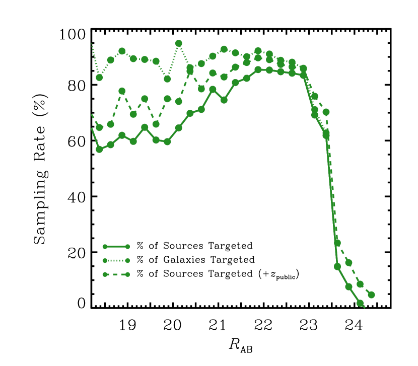 Figure 1.— The ACES target sampling rate as a function of -band
magnitude across the entire
COMBO-17/CDFS footprint. The target sampling rate is defined as the
percentage of objects at a given -band magnitude in the COMBO-17
photometric catalog that were observed by ACES. The dotted and
dashed lines show the sampling rate when only considering sources
classified as non-stellar in the COMBO-17 catalog5 (dotted) and
when accounting for sources with a published spectroscopic redshift
in the literature (dashed – see §2). At bright
magnitudes, , ACES brings the target sampling rate
in the CDFS to .
55footnotetext: To select the galaxy population,
all sources classified as “Star” or “WDwarf” in the COMBO-17
photometric catalog of Wolf et al. (2004) are excluded.
Figure 1.— The ACES target sampling rate as a function of -band
magnitude across the entire
COMBO-17/CDFS footprint. The target sampling rate is defined as the
percentage of objects at a given -band magnitude in the COMBO-17
photometric catalog that were observed by ACES. The dotted and
dashed lines show the sampling rate when only considering sources
classified as non-stellar in the COMBO-17 catalog5 (dotted) and
when accounting for sources with a published spectroscopic redshift
in the literature (dashed – see §2). At bright
magnitudes, , ACES brings the target sampling rate
in the CDFS to .
55footnotetext: To select the galaxy population,
all sources classified as “Star” or “WDwarf” in the COMBO-17
photometric catalog of Wolf et al. (2004) are excluded.
2. Target Selection and Slitmask Design
The ACES target sample is drawn from the COMBO-17 photometric catalog of Wolf et al. (2004, see also ). The primary spectroscopic sample is magnitude limited at , plus a significant population of fainter sources down to . Altogether, ACES observations spanned four separate observing seasons (2007B – 2010B), with the details of the target-selection algorithm and slitmask-design parameters varying from year to year. Here, we highlight the critical elements of the composite target population and slitmasks, including any significant variations from mask to mask. As stated above, the primary target sample for ACES was selected according to an -band magnitude limit of . Selecting in (versus a redder passband such as or ) ensures the highest possible signal-to-noise ratio in the continuum of the resulting optical spectra, and thus a high redshift-success rate for the survey. The given magnitude limit was adopted to enable a high level of completeness to be reached across the entire CDFS area. Moreover, at , the limit reaches along the red sequence and magnitude fainter than in the blue cloud population (Willmer et al., 2006), thereby enabling ACES to probe the systems that dominate the galaxy luminosity density and global star-formation rate at . As shown in Figure 1, ACES is highly-complete at , achieving a targeting rate of across the extended CDFS. In addition to the main target sample, we prioritized m sources detected as part of the Far-Infrared Deep Extragalactic Legacy (FIDEL) Survey (PI: M. Dickinson), which surveyed the CDFS to extremely deep flux limits at both m and m with Spitzer/MIPS (Magnelli et al., 2009, 2011). In selecting the optical counterparts to the m sources, we utilized a fainter magnitude limit of , targeting multiple optical sources in cases for which the identity of the optical counterpart was ambiguous. In total, ACES prioritized sources as m counterparts, with of these sources also meeting the primary magnitude limit for the survey. For the m-selected target population, our redshift success rate is quite high ( versus for the full target population). As a filler population in the target-selection process, we also included (with a lower selection probability) all sources down to the secondary magnitude limit of . These fainter, optically-selected sources comprise roughly of the total unique target sample (i.e, sources). The limit was adopted to match that of the DEEP2 Survey and allows the ACES dataset to probe even farther down the galaxy luminosity function at . To maximize the sampling density of the survey at , stellar sources were down-weighted in the target selection process. Stars were identified according to the spectral classification of Wolf et al. (2004), which utilized template SED fits to the -band photometry of COMBO-17. All sources classified as “Star” or “WDwarf” by Wolf et al. (2004) were down-weighted in the target selection. This included a total of sources at , of which we targeted obtaining secure redshifts for . As illustrated in Figure 1, these stellar sources are only a significant contribution to the total -band number counts at bright magnitudes; excluding this population of stars from the accounting, ACES targets of sources at . In selecting the ACES spectroscopic targets, we also down-weighted many sources with an existing spectroscopic redshift in the literature. This sample of “public” redshifts was drawn from Le Fèvre et al. (2004), Vanzella et al. (2005, 2006), Mignoli et al. (2005), Ravikumar et al. (2007), Szokoly et al. (2004), Popesso et al. (2009), and Balestra et al. (2010) as well as a small set of proprietary redshifts measured by the DEEP2 Galaxy Redshift Survey using Keck/DEIMOS. In all cases, only secure redshifts were employed. For example, only quality “A” and “B” (not “C”) redshifts were included from Vanzella et al. (2005, 2006); Popesso et al. (2009); Balestra et al. (2010). At , a total of unique sources with a spectroscopic redshift were down-weighted in the target selection process, with of these sources at . A significant number of objects () in this public catalog were observed by ACES; a comparison of the ACES redshift measurements to those previously published is presented in §4. Note that some of these public redshifts (most notably those of Balestra et al. 2010) were not yet published prior to the commencement of ACES, but were included in the target selection process as the survey progressed. Also, the distribution of the existing spectroscopic redshifts on the sky is strongly biased towards the center of the extended CDFS, primarily covering the smaller GOODS-S region (see Fig. 3).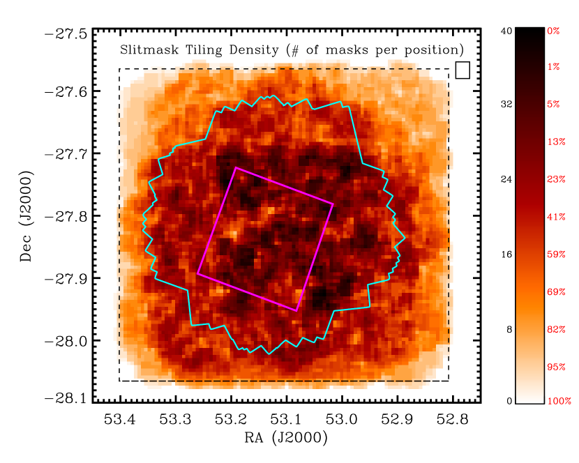 Figure 2.— The number of Magellan/IMACS slitmasks covering a given
spatial location (computed within a box of width and height ) as
a function of position within the CDFS. The red values to the right
of the color bar show the portion of the extended CDFS area (demarcated by the black dashed line
in the plot) that is covered by greater than the corresponding
number of slitmasks. ACES includes a total of slitmasks, with
of the field covered by at least 8 slitmasks. Finally, the
magenta and cyan outlines indicate the location of the CANDELS HST/WFC3-IR and 2-Ms Chandra/ACIS-I observations,
respectively. Every object in the field has multiple chances to be
placed on an ACES slitmask, helping to achieve a high sampling
density and minimize any bias against objects in overdense regions
on the sky.
For the 2007B through 2009B observing seasons, slitmasks were designed
in pairs, sharing a common position and orientation. By placing two
masks at the same location on the sky, objects had multiple chances to
be included on a slitmask (and thus observed). Furthermore, we were
able to integrate longer on fainter targets by including those sources
on both of the masks at a given position, while only including
brighter sources on a single mask and thus maximizing the number of
sources observed. As discussed in §6, data for
objects appearing on multiple slitmasks have yet to be combined; at
present, each slitmask is analyzed independently, such that there are
a higher number of repeated observations of some objects (especially
fainter targets).
Figure 2.— The number of Magellan/IMACS slitmasks covering a given
spatial location (computed within a box of width and height ) as
a function of position within the CDFS. The red values to the right
of the color bar show the portion of the extended CDFS area (demarcated by the black dashed line
in the plot) that is covered by greater than the corresponding
number of slitmasks. ACES includes a total of slitmasks, with
of the field covered by at least 8 slitmasks. Finally, the
magenta and cyan outlines indicate the location of the CANDELS HST/WFC3-IR and 2-Ms Chandra/ACIS-I observations,
respectively. Every object in the field has multiple chances to be
placed on an ACES slitmask, helping to achieve a high sampling
density and minimize any bias against objects in overdense regions
on the sky.
For the 2007B through 2009B observing seasons, slitmasks were designed
in pairs, sharing a common position and orientation. By placing two
masks at the same location on the sky, objects had multiple chances to
be included on a slitmask (and thus observed). Furthermore, we were
able to integrate longer on fainter targets by including those sources
on both of the masks at a given position, while only including
brighter sources on a single mask and thus maximizing the number of
sources observed. As discussed in §6, data for
objects appearing on multiple slitmasks have yet to be combined; at
present, each slitmask is analyzed independently, such that there are
a higher number of repeated observations of some objects (especially
fainter targets).
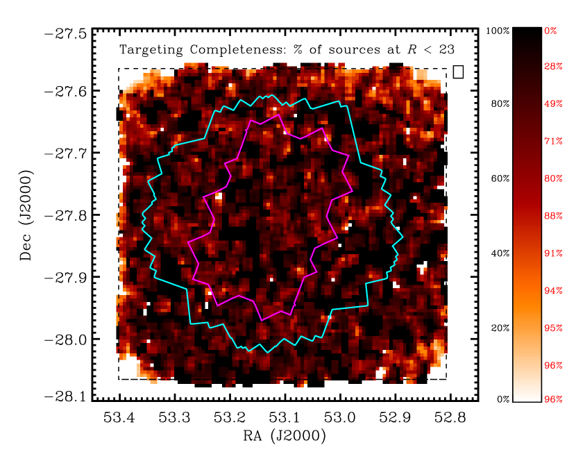
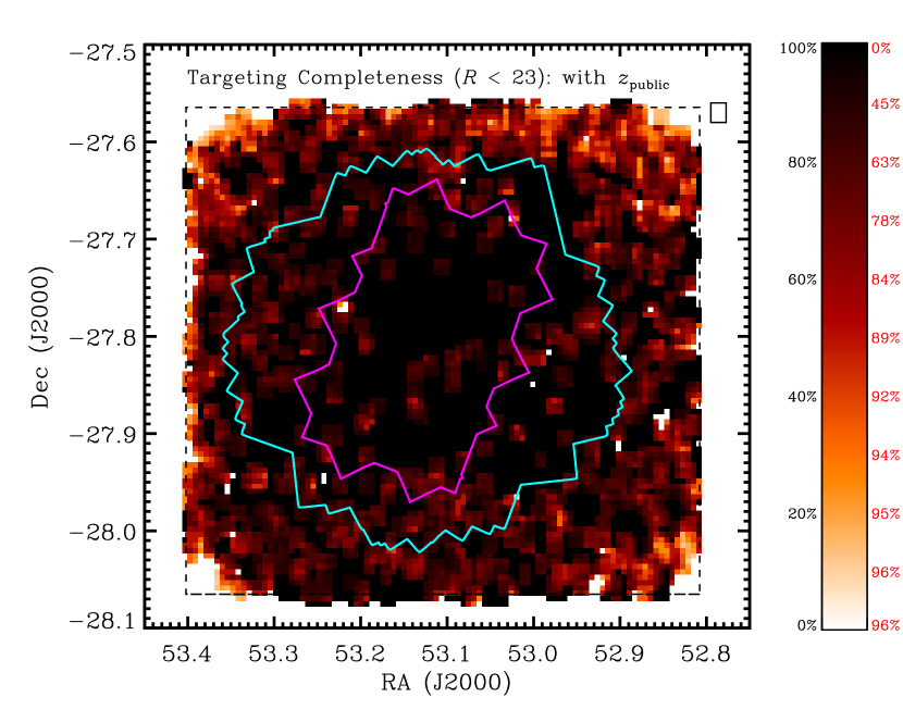 Figure 3.— The target sampling rate at for the ACES
target sample alone (left) and for the joint population
comprised of the ACES target sample and the set of existing public
redshifts detailed in §2 (right), computed
in a sliding box of width and
height . The size and shape of the
box are illustrated in the upper right-hand corner of each plot. The
associated color bars give the mapping from color to target
completeness (where black and white correspond to and
completeness, respectively) and completeness is defined as the
percentage of sources in the COMBO-17 imaging catalog with (including stars) targeted by ACES (or ACES plus the set
of sources with existing published redshifts). The red values to the
right of each color bar show the portion of the extended CDFS area (demarcated by the black dashed line
in each plot) that has a target completeness greater than the
corresponding level. Finally, the magenta and cyan outlines indicate
the location of the GOODS HST/ACS and 2-Ms Chandra/ACIS-I observations, respectively. At , the
sampling rate is exceptionally high ( from ACES
alone) across nearly the entire extended CDFS.
The tiling scheme for the IMACS slitmasks was designed to cover
the extended area of the
extended CDFS, with the caveat that the position and orientation of
each slitmask was dictated by the availability of suitably bright
stars for guiding and dynamic focusing.666Note that the
Magellan-Baade telescope includes an atmospheric dispersion
corrector (ADC) for the f/11 Nasmyth position of IMACS. A moderate
resolution grism and wide-band (–Å) filter were
employed in the observations (see §3), allowing
multiple (–) targets to occupy a given spatial position on a
slitmask and thereby enable upwards of sources to be
observed on a single slitmask. The average number of targets per mask
was , with the details of the slitmask design varying
slightly from year to year of observing.
For all of the ACES slitmasks, a standard slitwidth
was employed, with a minimum slitlength of
(centered on the target) and a gap of at least
between slits. For a subset of the slitmasks, slits were extended to
fill otherwise unoccupied real estate on the slitmask. On every mask,
the set of possible targets was restricted to those sources for which
the entire spectral range of –Å would fall on the
detector, given the position and orientation of the mask. The location
of the slitmasks on the sky was selected such that the full area of
the mask would fall within the CDFS region, leading to a slitmask
tiling scheme that more highly samples the central portion of the
field. This relative oversampling is a direct product of the large
size of the IMACS field-of-view at f/2 ( unvignetted); any IMACS slitmask that falls entirely
within the extended CDFS region will overlap the central portion of
the CDFS, independent of orientation. As shown in Figure
2, the number of ACES slitmasks at a given position
within the CDFS varies significantly from at the
center of the field to at the edges.
In spite of this spatial variation in the total sampling rate, ACES
achieves a relatively uniform spatial sampling rate for the main galaxy sample. As evident in Figure 3, ACES
targets of sources at , relatively
independent of position within the CDFS. When including spectroscopic
observations from the literature (counting the associated objects as
being observed), the target sampling is remarkably complete at , with roughly half of the
CDFS surveyed to completeness. This relatively high and
uniform sampling rate is critical for the ability to measure local
environments with the ACES dataset.
Figure 3.— The target sampling rate at for the ACES
target sample alone (left) and for the joint population
comprised of the ACES target sample and the set of existing public
redshifts detailed in §2 (right), computed
in a sliding box of width and
height . The size and shape of the
box are illustrated in the upper right-hand corner of each plot. The
associated color bars give the mapping from color to target
completeness (where black and white correspond to and
completeness, respectively) and completeness is defined as the
percentage of sources in the COMBO-17 imaging catalog with (including stars) targeted by ACES (or ACES plus the set
of sources with existing published redshifts). The red values to the
right of each color bar show the portion of the extended CDFS area (demarcated by the black dashed line
in each plot) that has a target completeness greater than the
corresponding level. Finally, the magenta and cyan outlines indicate
the location of the GOODS HST/ACS and 2-Ms Chandra/ACIS-I observations, respectively. At , the
sampling rate is exceptionally high ( from ACES
alone) across nearly the entire extended CDFS.
The tiling scheme for the IMACS slitmasks was designed to cover
the extended area of the
extended CDFS, with the caveat that the position and orientation of
each slitmask was dictated by the availability of suitably bright
stars for guiding and dynamic focusing.666Note that the
Magellan-Baade telescope includes an atmospheric dispersion
corrector (ADC) for the f/11 Nasmyth position of IMACS. A moderate
resolution grism and wide-band (–Å) filter were
employed in the observations (see §3), allowing
multiple (–) targets to occupy a given spatial position on a
slitmask and thereby enable upwards of sources to be
observed on a single slitmask. The average number of targets per mask
was , with the details of the slitmask design varying
slightly from year to year of observing.
For all of the ACES slitmasks, a standard slitwidth
was employed, with a minimum slitlength of
(centered on the target) and a gap of at least
between slits. For a subset of the slitmasks, slits were extended to
fill otherwise unoccupied real estate on the slitmask. On every mask,
the set of possible targets was restricted to those sources for which
the entire spectral range of –Å would fall on the
detector, given the position and orientation of the mask. The location
of the slitmasks on the sky was selected such that the full area of
the mask would fall within the CDFS region, leading to a slitmask
tiling scheme that more highly samples the central portion of the
field. This relative oversampling is a direct product of the large
size of the IMACS field-of-view at f/2 ( unvignetted); any IMACS slitmask that falls entirely
within the extended CDFS region will overlap the central portion of
the CDFS, independent of orientation. As shown in Figure
2, the number of ACES slitmasks at a given position
within the CDFS varies significantly from at the
center of the field to at the edges.
In spite of this spatial variation in the total sampling rate, ACES
achieves a relatively uniform spatial sampling rate for the main galaxy sample. As evident in Figure 3, ACES
targets of sources at , relatively
independent of position within the CDFS. When including spectroscopic
observations from the literature (counting the associated objects as
being observed), the target sampling is remarkably complete at , with roughly half of the
CDFS surveyed to completeness. This relatively high and
uniform sampling rate is critical for the ability to measure local
environments with the ACES dataset.
3. Observations and Data Reduction
ACES spectroscopic observations employed the f/2 camera in the Inamori-Magellan Areal Camera and Spectrograph (IMACS) on the Magellan-Baade telescope and were completed across four separate observing seasons (2007B – 2010B) as detailed in Table 1. The instrument set-up included the 200 lines mm-1 grism (blaze angle of ) in conjunction with the WB5650–9200 wide-band filter, which yields a nominal spectral coverage of –Å at a resolution of (at Å). Each slitmask was observed for a total integration time of – sec, divided into (at least) – individual – sec integrations (with no dithering performed) to facilitate the rejection of cosmic rays — see Table 1 for details regarding the total integration times. Immediately following each set of science exposures (i.e., without moving the telescope or modifying the instrument configuration), a quartz flat-field frame and comparison arc spectrum (using He, Ar, Ne) were taken to account for instrument flexure and detector fringing. There are two notable variations in the instrument configuration that occurred in the course of the ACES observations. Between the 2007B (January 2008) and 2008B (November 2008) observing seasons, the IMACS CCDs were upgraded from the original SITe to deep-depletion E2V chips (Dressler et al., 2011). The new CCDs provided much improved quantum efficiency, especially at red wavelengths. In addition to the detector update, for the initial observing run (in January 2008), the data were collected using the incorrect grism. Instead of the 200 lines mm-1 grism, the higher-resolution 300 lines mm-1 grism (blaze angle of ) was installed in IMACS. The resulting spectra from those slitmasks (ACES1–ACES8) are therefore at slightly higher resolution ( at Å). Given that the slitmasks multiplex in the spectral (in addition to the spatial) direction and were designed for use with the lower-resolution grism, the spectra for many objects overlap significantly. In addition, for a subset of the objects (primarily those located closer to the edge of the slitmask), part of the –Å spectral window was dispersed off of the IMACS detector. In such instances, on the order of Å was typically lost at either the blue or red extreme of the spectral window. While the data taken on this first observing run were negatively impacted by the use of the incorrect grism (including a slight reduction in total throughput), redshifts were still able to be measured for many of the targets. In an attempt to maintain the uniformity of the dataset, however, the vast majority of the objects on the ACES1–ACES8 slitmasks (1166 of 1315 objects) were reobserved in subsequent observing seasons. Table 1 Slitmask Observation Information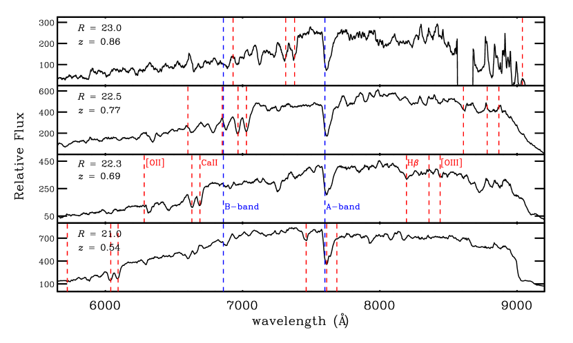
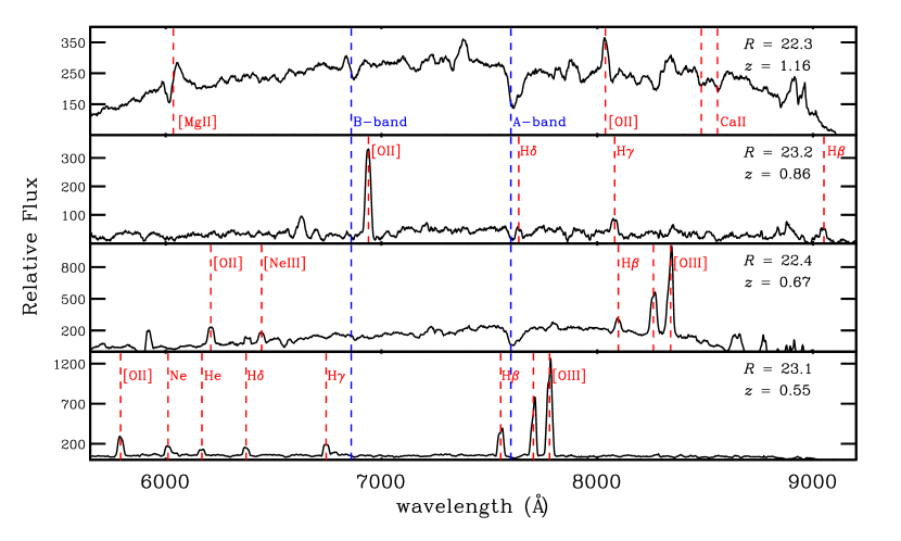 Figure 4.— Example ACES one-dimensional spectra of red and/or passive
galaxies (left) and star-forming/active galaxies
(right). The location of prominent spectral features as well
as the A- and B-band telluric features are indicated by the red and
blue dashed vertical lines, respectively. Note that the spectra have
been smoothed (weighted by the inverse variance) using a kernel of
pixels (or Å) in width.
The IMACS spectroscopic observations were reduced using the COSMOS
data reduction pipeline developed at the Carnegie Observatories
(Dressler et al., 2011).777http://obs.carnegiescience.edu/Code/cosmos
For each slitlet, COSMOS yields a flat-fielded and sky-subtracted,
two-dimensional spectrum, with wavelength calibration performed by
fitting to the arc lamp emission lines. One-dimensional spectra were
extracted and redshifts were measured from the reduced spectra using
additional software developed as part of the DEEP2 Galaxy Redshift
Survey and adapted for use with IMACS as part of ACES and as part of
the spectroscopic follow-up of the Red-Sequence Cluster Survey (RCS,
Gladders & Yee 2005; RCS, Yan et al. in prep). A detailed
description of the DEEP2 reduction packages (spec2d and spec1d) is presented in Cooper et al. (2012a) and Newman et al. (2012).
Example spectra for objects spanning a broad range of galaxy type and
apparent magnitude are shown in Figure 4. All spectra
were visually inspected by M. Cooper, with a quality code
assigned corresponding to the accuracy of the redshift value — denote secure redshifts, with corresponding to stellar
sources and denoting secure galaxy redshifts (see Table
2). Confirmation of multiple spectral features was
generally required to assign a quality code of or . As
discussed in §4.2, and redshifts are
estimated to be and reliable,
respectively. Quality codes of are assigned to observations
that yield no useful redshift information () or may possibly
yield redshift information after further analysis or re-reduction of
the data (). For detailed descriptions of the reduction pipeline,
redshift measurement code, and quality assignment process refer to
Wirth et al. (2004), Davis et al. (2007), and Newman et al. (2012).
Figure 4.— Example ACES one-dimensional spectra of red and/or passive
galaxies (left) and star-forming/active galaxies
(right). The location of prominent spectral features as well
as the A- and B-band telluric features are indicated by the red and
blue dashed vertical lines, respectively. Note that the spectra have
been smoothed (weighted by the inverse variance) using a kernel of
pixels (or Å) in width.
The IMACS spectroscopic observations were reduced using the COSMOS
data reduction pipeline developed at the Carnegie Observatories
(Dressler et al., 2011).777http://obs.carnegiescience.edu/Code/cosmos
For each slitlet, COSMOS yields a flat-fielded and sky-subtracted,
two-dimensional spectrum, with wavelength calibration performed by
fitting to the arc lamp emission lines. One-dimensional spectra were
extracted and redshifts were measured from the reduced spectra using
additional software developed as part of the DEEP2 Galaxy Redshift
Survey and adapted for use with IMACS as part of ACES and as part of
the spectroscopic follow-up of the Red-Sequence Cluster Survey (RCS,
Gladders & Yee 2005; RCS, Yan et al. in prep). A detailed
description of the DEEP2 reduction packages (spec2d and spec1d) is presented in Cooper et al. (2012a) and Newman et al. (2012).
Example spectra for objects spanning a broad range of galaxy type and
apparent magnitude are shown in Figure 4. All spectra
were visually inspected by M. Cooper, with a quality code
assigned corresponding to the accuracy of the redshift value — denote secure redshifts, with corresponding to stellar
sources and denoting secure galaxy redshifts (see Table
2). Confirmation of multiple spectral features was
generally required to assign a quality code of or . As
discussed in §4.2, and redshifts are
estimated to be and reliable,
respectively. Quality codes of are assigned to observations
that yield no useful redshift information () or may possibly
yield redshift information after further analysis or re-reduction of
the data (). For detailed descriptions of the reduction pipeline,
redshift measurement code, and quality assignment process refer to
Wirth et al. (2004), Davis et al. (2007), and Newman et al. (2012).
4. Redshift Catalog
A preliminary ACES redshift catalog is presented in Table 2, a subset of which is listed herein. The entirety of Table 2 appears in the electronic version of the Journal. Note that a redshift is only included when classified as being secure, . The total number of secure redshifts in the sample is out of total, unique targets. The redshift distribution for this sample, as shown in Figure 5, is biased towards with a tail out to higher redshift.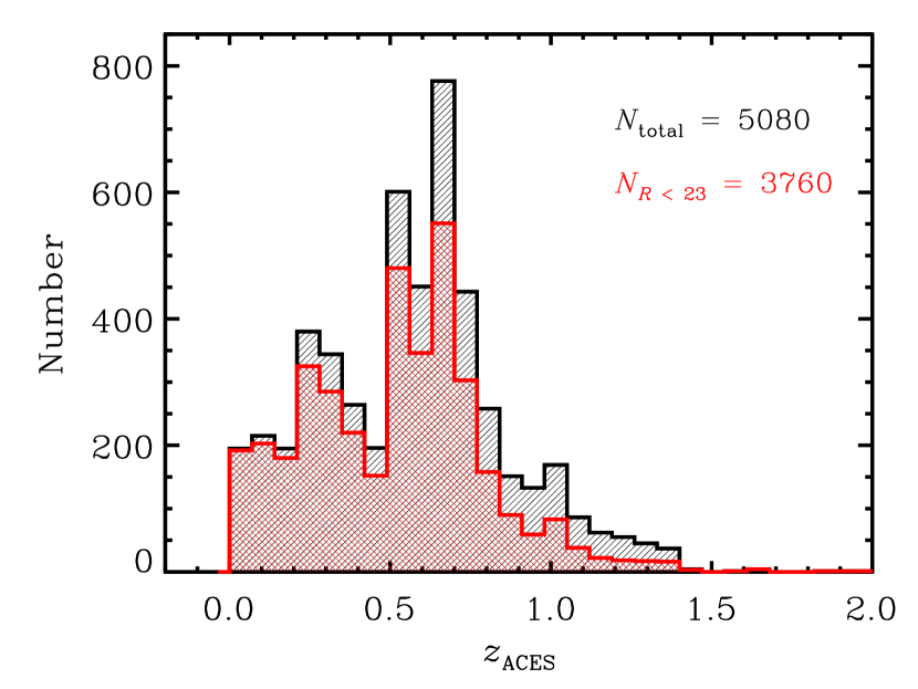 Figure 5.— The distribution of the unique, secure
redshifts measured by ACES (black histogram). The red histogram
shows the distribution for the main target sample. The
main sample is biased towards , with a tail to
higher redshift.
At bright magnitudes (), ACES is highy complete,
obtaining a secure redshift for of all sources
within the COMBO-17/CDFS
footprint (see Fig. 6). When excluding sources
identified as stars by COMBO-17 ( sources; see §2) and including published spectroscopic redshifts from
the literature, the redshift completeness exceeds at the very
brightest magnitudes ().
Figure 5.— The distribution of the unique, secure
redshifts measured by ACES (black histogram). The red histogram
shows the distribution for the main target sample. The
main sample is biased towards , with a tail to
higher redshift.
At bright magnitudes (), ACES is highy complete,
obtaining a secure redshift for of all sources
within the COMBO-17/CDFS
footprint (see Fig. 6). When excluding sources
identified as stars by COMBO-17 ( sources; see §2) and including published spectroscopic redshifts from
the literature, the redshift completeness exceeds at the very
brightest magnitudes ().
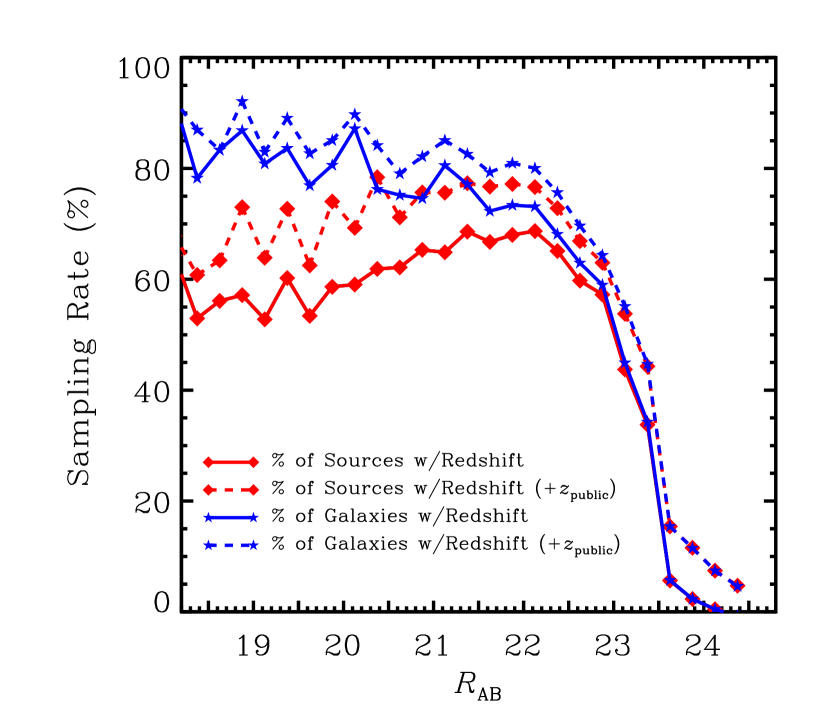 Figure 6.— The ACES redshift success rate as a function of -band
magnitude computed for all sources within the COMBO-17/CDFS footprint (solid red line). The
redshift success rate is defined as the percentage of objects at a
given -band magnitude in the COMBO-17 photometric catalog
(including stars) that were observed by ACES and yielded a secure
(,, – see §4) redshift. The solid blue
line shows the redshift completeness when only considering sources
classified as non-stellar in the COMBO-17 catalog. At bright
magnitudes, , the ACES sample is highly
complete. The corresponding red and blue dashed lines show the
associated completeness when accounting for sources with a published
spectroscopic redshift in the literature (see §2).
As discussed in §2, the ACES catalog has a high
number of repeated observations. These independent observations
provide a direct means for determining the precision of the redshift
measurements. As shown in Figure 7, we find a scatter
of km s-1 within the ACES sample when
comparing repeat observations of a sizable sample of secure
redshifts. The scatter is found to be independent of the redshift
quality (i.e., versus ). While the precision of the
ACES redshifts is poorer than that of surveys such as DEEP2 and DEEP3,
it is adequate for characterizing local environments (Cooper et al., 2005)
as well as identifying and measuring the velocity dispersions of
galaxy groups.
Figure 6.— The ACES redshift success rate as a function of -band
magnitude computed for all sources within the COMBO-17/CDFS footprint (solid red line). The
redshift success rate is defined as the percentage of objects at a
given -band magnitude in the COMBO-17 photometric catalog
(including stars) that were observed by ACES and yielded a secure
(,, – see §4) redshift. The solid blue
line shows the redshift completeness when only considering sources
classified as non-stellar in the COMBO-17 catalog. At bright
magnitudes, , the ACES sample is highly
complete. The corresponding red and blue dashed lines show the
associated completeness when accounting for sources with a published
spectroscopic redshift in the literature (see §2).
As discussed in §2, the ACES catalog has a high
number of repeated observations. These independent observations
provide a direct means for determining the precision of the redshift
measurements. As shown in Figure 7, we find a scatter
of km s-1 within the ACES sample when
comparing repeat observations of a sizable sample of secure
redshifts. The scatter is found to be independent of the redshift
quality (i.e., versus ). While the precision of the
ACES redshifts is poorer than that of surveys such as DEEP2 and DEEP3,
it is adequate for characterizing local environments (Cooper et al., 2005)
as well as identifying and measuring the velocity dispersions of
galaxy groups.
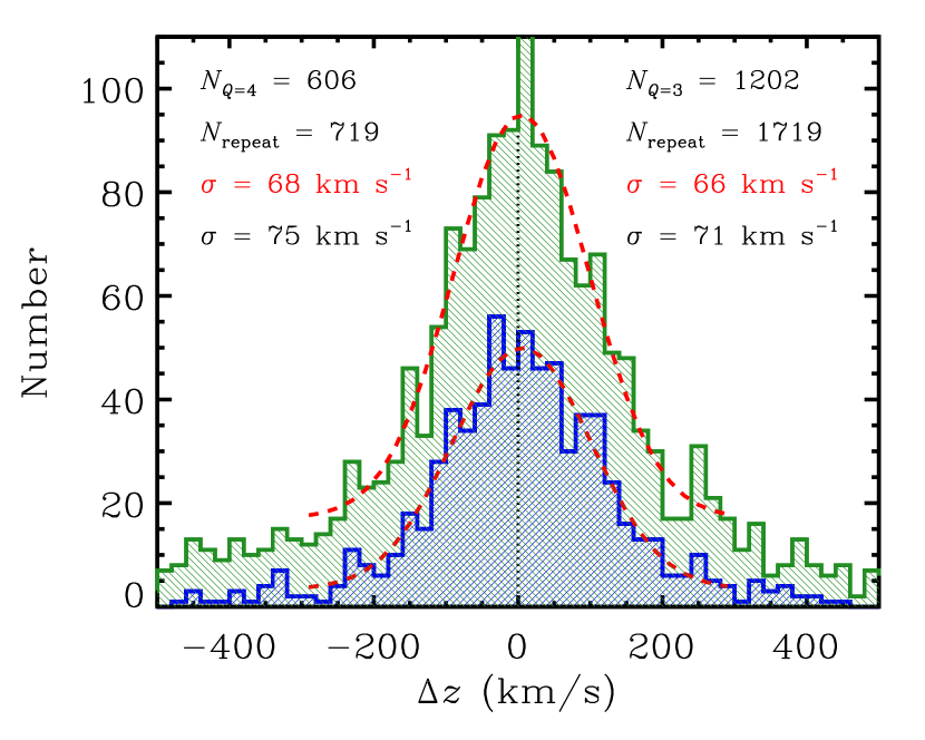 Figure 7.— The distribution of velocity differences computed from
repeated observations, where both observations of a given galaxy
yielded a (blue histogram) or redshift (green
histogram). A total of and unique sources comprise the
two distributions separately. The dispersion as given by a
Gaussian-fit to the distribution (red dashed line) and by the square
root of the second moment of the distribution are reported in red
and black font (or top and bottom numbers), respectively. A total of
pairs of observations comprise the two distributions, with a
dispersion of km s-1 independent of redshift
quality.
Figure 7.— The distribution of velocity differences computed from
repeated observations, where both observations of a given galaxy
yielded a (blue histogram) or redshift (green
histogram). A total of and unique sources comprise the
two distributions separately. The dispersion as given by a
Gaussian-fit to the distribution (red dashed line) and by the square
root of the second moment of the distribution are reported in red
and black font (or top and bottom numbers), respectively. A total of
pairs of observations comprise the two distributions, with a
dispersion of km s-1 independent of redshift
quality.
4.1. Comparison to Photometric Redshift Samples
The ACES spectroscopic sample provides an excellent dataset with which to test the precision of the COMBO-17 photometric redshift measurements. The COMBO-17 photo- estimates are based on -band photometry spanning 3500Å to 9300Å. While their accuracy at higher redshift is impacted significantly by the lack of near-IR observations, the COMBO-17 photometric redshifts are very robust at . Based on a comparison to a relatively small (, primarily at ) sample of spectroscopic redshifts, Wolf et al. (2004) found a - error of , with a less than catastrophic failure rate (where failure is defined to be ). In Figure 8, we directly compare the COMBO-17 photometric redshifts to the ACES spectroscopic redshifts for all sources with a secure (,,) redshift. The deficiency of objects at results largely from the inability of ACES to resolve the [O II] doublet. That is, the ACES spectrum of an emission-line galaxy at would yield an unresolved [O II] emission doublet at Å, while H and [O III] would be redward of our spectral window (Å). We are unable to easily distinguish this single emission line from H (i.e., a galaxy at ), as at that redshift H and [O III] would be blueward of our spectral window (Å). As a result, many objects at are classified as . Using broad-band color info, we hope to recover these objects in the future (e.g., Kirby et al., 2007). Within the ACES dataset alone, there are objects with a secure galaxy redshift (i.e., ,) and a photometric redshift in the catalog of Wolf et al. (2004). For this set of objects, the COMBO-17 photometric redshifts exhibit a dispersion of (with - outliers removed) and a catastrophic failure rate (again taken to be ) of . As highlighted by Wolf et al. (2004), however, the COMBO-17 photometric redshifts degrade in quality for increasingly fainter galaxies, and the ACES sample extends to . For bright objects (), the dispersion relative to the ACES spectroscopic redshifts is (again with - outliers removed), with a catastrophic failure rate of . The precision is slightly poorer at fainter magnitudes (), increasing to , while at the faintest magnitudes probed by ACES, the scatter between the COMBO-17 photo- values and our spectroscopic redshifts increases to (for ). For the main sample, the catastrophic failure rate () is . These trends with apparent magnitude and redshift are evident in Figure 9, which shows the dependence of the photometric redshift error and the catastrophic failure rate on -band magnitude, redshift, and observed color based on a comparison of the ACES spectroscopic redshift and COMBO-17 photometric redshift catalogs. At faint magnitudes and at higher redshift , the photometric-redshift errors and failure rates for COMBO-17 increase significantly. However, we find no significant correlation between the quality of the photometric redshifts and apparent color, suggesting that there is little dependence on the spectral-type or star-formation history of a galaxy.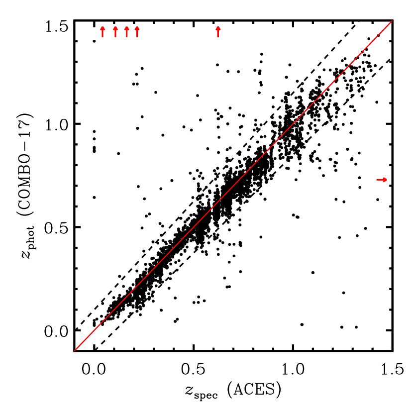 Figure 8.— A comparison of the spectroscopic redshifts from ACES to the
photometric redshifts of COMBO-17 (Wolf et al., 2004). In general, the
agreement is quite good, with a dispersion of (with - outliers removed) for the galaxy
(,) sample. The red vertical arrows indicate sources for
which the photometric redshift value is greater than , in
conflict with the spectroscopic value, which is indicated by the
position of the arrow (and vice versa for the red horizontal
arrow). The dashed black lines correspond to a nominal catastrophic
failure level of .
As highlighted earlier, the degradation in photo- quality with
redshift is in part due to the lack of near-IR photometry in the
multi-band imaging of COMBO-17. In contrast, the photometric redshifts
from the Multiwavelength Survey by Yale-Chile
(MUSYC, Gawiser et al., 2006), as computed by Cardamone et al. (2010),
include broad-band optical and near-IR () imaging in addition to
photometry in medium-bands from Subaru. As shown in Figure
9, the MUSYC photometric redshifts exhibit much
smaller scatter in relation to the ACES spectroscopic redshift sample,
with across the full magnitude and
redshift range probed. In addition, the catastrophic failure rate for
the MUSYC sample is roughly a factor of lower than that found for
the COMBO-17 photometric redshift catalog.
Figure 8.— A comparison of the spectroscopic redshifts from ACES to the
photometric redshifts of COMBO-17 (Wolf et al., 2004). In general, the
agreement is quite good, with a dispersion of (with - outliers removed) for the galaxy
(,) sample. The red vertical arrows indicate sources for
which the photometric redshift value is greater than , in
conflict with the spectroscopic value, which is indicated by the
position of the arrow (and vice versa for the red horizontal
arrow). The dashed black lines correspond to a nominal catastrophic
failure level of .
As highlighted earlier, the degradation in photo- quality with
redshift is in part due to the lack of near-IR photometry in the
multi-band imaging of COMBO-17. In contrast, the photometric redshifts
from the Multiwavelength Survey by Yale-Chile
(MUSYC, Gawiser et al., 2006), as computed by Cardamone et al. (2010),
include broad-band optical and near-IR () imaging in addition to
photometry in medium-bands from Subaru. As shown in Figure
9, the MUSYC photometric redshifts exhibit much
smaller scatter in relation to the ACES spectroscopic redshift sample,
with across the full magnitude and
redshift range probed. In addition, the catastrophic failure rate for
the MUSYC sample is roughly a factor of lower than that found for
the COMBO-17 photometric redshift catalog.
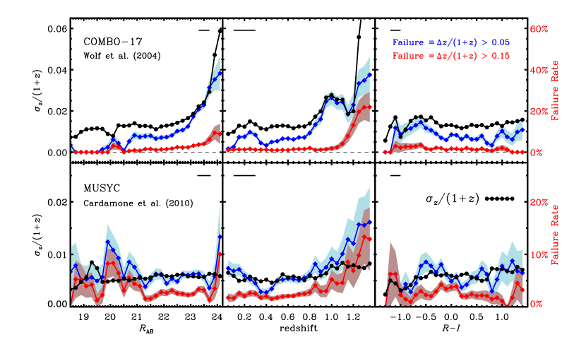 Figure 9.— The dependence of the photometric redshift error and the catastrophic failure rate on -band magnitude
(left), redshift (middle), and observed color
(right) for the COMBO-17 (top) and MUSYC
(bottom) photometric redshift catalogs. The errors (black
points) and failure rates (blue and red diamonds) are computed using
sliding boxes with widths given by the black dashes in the upper
corner of each plot, while the light blue and red shaded regions
denote the uncertainty on the respective failure rates, as
given by binomial statistics. In all cases, the dispersions
are computed with outliers
removed. In determining the redshift and color dependences, only
objects with are included. For COMBO-17, the photo-
errors and failure rates increase significantly at fainter
magnitudes and higher redshift , while the
trends are much weaker for the MUSYC photometric
redshifts.
Figure 9.— The dependence of the photometric redshift error and the catastrophic failure rate on -band magnitude
(left), redshift (middle), and observed color
(right) for the COMBO-17 (top) and MUSYC
(bottom) photometric redshift catalogs. The errors (black
points) and failure rates (blue and red diamonds) are computed using
sliding boxes with widths given by the black dashes in the upper
corner of each plot, while the light blue and red shaded regions
denote the uncertainty on the respective failure rates, as
given by binomial statistics. In all cases, the dispersions
are computed with outliers
removed. In determining the redshift and color dependences, only
objects with are included. For COMBO-17, the photo-
errors and failure rates increase significantly at fainter
magnitudes and higher redshift , while the
trends are much weaker for the MUSYC photometric
redshifts.
4.2. Comparison to Spectroscopic Redshift Samples
Matching our catalog to previously-published spectroscopic redshifts in the field (e.g., Le Fèvre et al., 2004; Vanzella et al., 2005, 2006; Balestra et al., 2010, see §2), we find of our targets have a redshift published as part of these existing datasets. For of these objects, we measure a secure redshift from our IMACS spectroscopy. The agreement between the ACES redshifts and those in the literature is generally good. We find a median offset of km s-1 when comparing to the “public” redshift catalog detailed in §2. For the small set of significant outliers (the objects with km s-1), the ACES spectra were re-examined to confirm the validity of the ACES redshifts. While some outliers could be the result of mismatching between the ACES catalog and the public databases, the majority are the result of line misidentification (e.g., confusing H with [O II]) or some other failure in redshift identification (see Figure 10). The significant overlap between the ACES sample and the set of existing redshifts in the literature also provides a means to conservatively estimate the reliability of the ACES redshifts. Taking the previously-published values to be the true redshift for each galaxy, we measure the catastrophic failure rate ( km s-1) for the and ACES redshifts. For the sources with and source with redshifts in the ACES catalog, we find failure rates of and , respectively. As shown in Figure 10, some of the previously-published redshifts are clearly in error, thus these confidence values are conservative estimates. Comparing within the ACES sample alone, we find that and of sources with repeated observations (both yielding and redshifts — see Fig. 7) have redshifts measurements that disagree at greater than km s-1.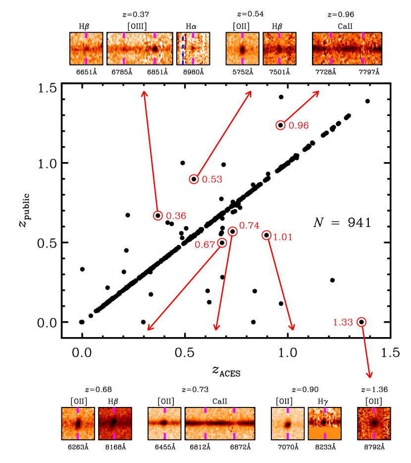 Figure 10.— For the sample of objects with a secure redshift in
ACES (i.e., , , or ) and also a secure measurement in
the literature, we plot a comparison of the two spectroscopic
redshift measurements. The agreement is quite good, with only
objects having redshift measurements that disagree at km s-1. For of these outliers, we show cut-outs from
the Magellan/IMACS two-dimensional spectra, illustrating the
spectral features that confirm the ACES redshift. In each case, the
COMBO-17 photometric redshift (given in red font within the plot)
agrees quite well with the ACES spectroscopic redshift. Refer to §4 for details regarding the set of “public” redshift
measurements.
The new redshifts presented here should significantly enhance studies
of galaxy evolution and cosmology in the CDFS. Our sample expands upon
previous spectroscopic work in the field, significantly increasing the
size of the existing redshift database. Furthermore, our observations
broaden the area covered, extending beyond the GOODS-S HST/ACS
footprint, allowing us to target a greater number of relatively rare
sources. In particular, we specifically targeted Spitzer/MIPS
m sources, including those observed by previous spectroscopic
efforts in the field. Within the FIDEL Survey’s Spitzer/MIPS
m photometric catalog for GOODS-S, which covers an area of
roughly , there are only sources
detected at mJy (Magnelli et al., 2011). The relatively small
number of these sources puts a premium on spectroscopic follow-up,
including those located outside of the GOODS-S area. The FIDEL Survey
covers a broader region surrounding the GOODS-S area, actually
extending significantly beyond the ACES footprint in most directions
when combined with existing Spitzer/MIPS observations. In total,
sources are detected (down to mJy) at m within the COMBO-17 footprint as part of the
FIDEL survey (requiring a - detection at both m and
m). As highlighted in §2, ACES targets
sources as potential optical counterparts to these sources (i.e.,
within of a m source).
The m observations conducted as part of the FIDEL Survey are
the deepest in the sky, allowing significant numbers of star-forming
galaxies and active galactic nuclei to be detected out to intermediate
redshift at rest-frame wavelengths that are dramatically less impacted
by aromatic and silicate emission than those normally probed by Spitzer/MIPS m observations. With accompanying redshift
information from spectroscopic follow-up such as presented here, these
deep far-infrared data provide a unique constraint on the cosmic
star-formation history at intermediate redshift
(e.g., Magnelli et al., 2009).
Figure 10.— For the sample of objects with a secure redshift in
ACES (i.e., , , or ) and also a secure measurement in
the literature, we plot a comparison of the two spectroscopic
redshift measurements. The agreement is quite good, with only
objects having redshift measurements that disagree at km s-1. For of these outliers, we show cut-outs from
the Magellan/IMACS two-dimensional spectra, illustrating the
spectral features that confirm the ACES redshift. In each case, the
COMBO-17 photometric redshift (given in red font within the plot)
agrees quite well with the ACES spectroscopic redshift. Refer to §4 for details regarding the set of “public” redshift
measurements.
The new redshifts presented here should significantly enhance studies
of galaxy evolution and cosmology in the CDFS. Our sample expands upon
previous spectroscopic work in the field, significantly increasing the
size of the existing redshift database. Furthermore, our observations
broaden the area covered, extending beyond the GOODS-S HST/ACS
footprint, allowing us to target a greater number of relatively rare
sources. In particular, we specifically targeted Spitzer/MIPS
m sources, including those observed by previous spectroscopic
efforts in the field. Within the FIDEL Survey’s Spitzer/MIPS
m photometric catalog for GOODS-S, which covers an area of
roughly , there are only sources
detected at mJy (Magnelli et al., 2011). The relatively small
number of these sources puts a premium on spectroscopic follow-up,
including those located outside of the GOODS-S area. The FIDEL Survey
covers a broader region surrounding the GOODS-S area, actually
extending significantly beyond the ACES footprint in most directions
when combined with existing Spitzer/MIPS observations. In total,
sources are detected (down to mJy) at m within the COMBO-17 footprint as part of the
FIDEL survey (requiring a - detection at both m and
m). As highlighted in §2, ACES targets
sources as potential optical counterparts to these sources (i.e.,
within of a m source).
The m observations conducted as part of the FIDEL Survey are
the deepest in the sky, allowing significant numbers of star-forming
galaxies and active galactic nuclei to be detected out to intermediate
redshift at rest-frame wavelengths that are dramatically less impacted
by aromatic and silicate emission than those normally probed by Spitzer/MIPS m observations. With accompanying redshift
information from spectroscopic follow-up such as presented here, these
deep far-infrared data provide a unique constraint on the cosmic
star-formation history at intermediate redshift
(e.g., Magnelli et al., 2009).
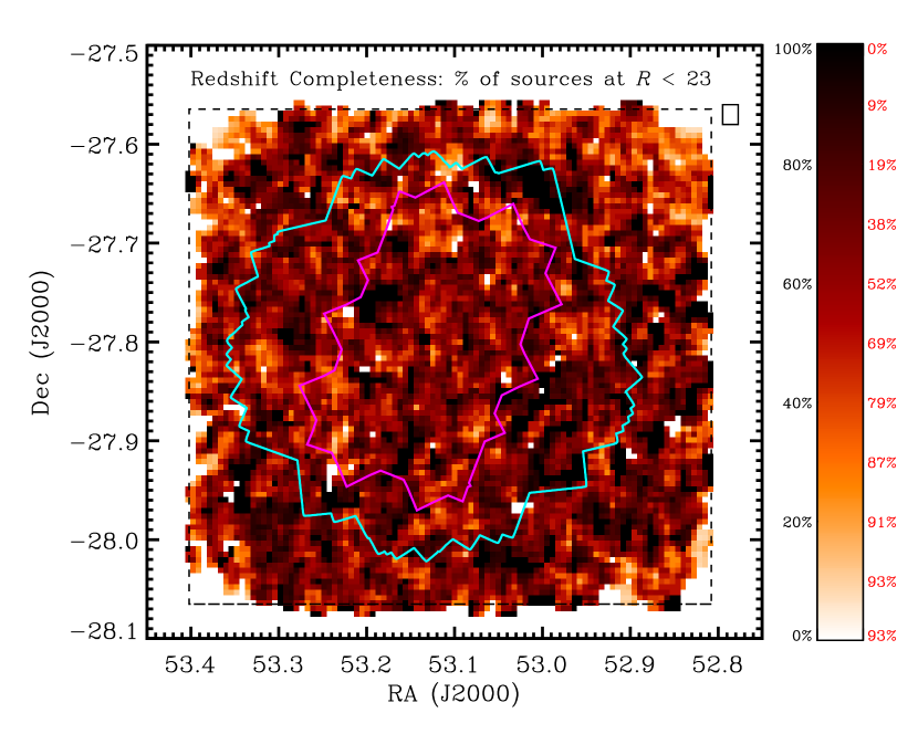
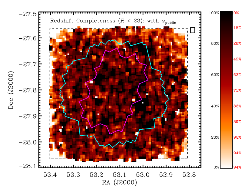 Figure 11.— The redshift completeness at for the ACES
sample alone (left) and for the joint population comprised by
ACES and the set of existing public redshifts detailed in §2 (right), computed in a sliding box of width
and height . The size and shape of the box are illustrated in
the upper right-hand corner of each plot. The associated color bars
give the mapping from color to redshift completeness (where black
and white correspond to and completeness,
respectively) and completeness is defined as the percentage of
sources in the COMBO-17 imaging catalog with
(including stars) for which ACES (or ACES plus the set of sources
with existing published redshifts) measured a secure redshift (i.e.,
). The red values to the right of each color bar show
the portion of the extended CDFS
area (demarcated by the black dashed line in each plot) that has a
redshift completeness greater than the corresponding level. Finally,
the magenta and cyan outlines denote the location of the GOODS
HST/ACS and 2-Ms Chandra/ACIS-I observations,
respectively. At , the redshift completeness is high
( from ACES alone) across nearly the entire
extended CDFS.
Table 2 ACES Redshift Catalog
Figure 11.— The redshift completeness at for the ACES
sample alone (left) and for the joint population comprised by
ACES and the set of existing public redshifts detailed in §2 (right), computed in a sliding box of width
and height . The size and shape of the box are illustrated in
the upper right-hand corner of each plot. The associated color bars
give the mapping from color to redshift completeness (where black
and white correspond to and completeness,
respectively) and completeness is defined as the percentage of
sources in the COMBO-17 imaging catalog with
(including stars) for which ACES (or ACES plus the set of sources
with existing published redshifts) measured a secure redshift (i.e.,
). The red values to the right of each color bar show
the portion of the extended CDFS
area (demarcated by the black dashed line in each plot) that has a
redshift completeness greater than the corresponding level. Finally,
the magenta and cyan outlines denote the location of the GOODS
HST/ACS and 2-Ms Chandra/ACIS-I observations,
respectively. At , the redshift completeness is high
( from ACES alone) across nearly the entire
extended CDFS.
Table 2 ACES Redshift Catalog5. Environment Measures
By extending beyond the GOODS-S footprint (i.e., the area primarily targeted by previous spectroscopic efforts in the field), ACES substantially expands the area over which galaxy overdensity (or “environment”) can be measured in the CDFS. The finite area of sky covered by a survey introduces geometric distortions — or edge effects — which bias environment measures near borders (or holes) in the survey field, generally leading to an underestimate of the local overdensity (Cooper et al., 2005, 2006). To minimize the impact of these edge effects on studies of environment, galaxies near the edge of the survey field (e.g., within a projected distance of - comoving Mpc of an edge) are often excluded from any analysis. As such, the ACES dataset, which spans a considerably larger region than previous spectroscopic samples (and with a much more spatially-uniform sampling rate, see Fig. 3 and Fig. 11), now allows the environment of galaxies at intermediate redshift to be accurately computed across nearly the entire area of the CDFS, thereby enabling unique analyses of small-scale clustering in one of the most well-studied extragalactic fields in the sky. For each galaxy in the ACES redshift catalog (see Table 2), we estimate the local galaxy overdensity, or “environment”, using measurements of the projected third-nearest-neighbor surface density () about each galaxy, where the surface density depends on the projected distance to the third-nearest neighbor, , as . Over quasi-linear regimes, the mass density and galaxy density should simply differ by a factor of the galaxy bias (Kaiser, 1987). In computing , only objects within a velocity window of km s-1 are counted, to exclude foreground and background galaxies along the line-of-sight. To explore any dependencies on the choice of in this -nearest-neighbor approach to measuring environment, we also compute overdensities based on the distance to the fourth- and fifth-nearest-neighbor (see Table 3). When estimating the local environment within a survey dataset, each surface density measurement must be corrected according to the redshift and spatial dependence of the survey’s sampling rate. To minimize the variation in the spatial component of the ACES sampling rate, we select the galaxy population as the tracer population by which the local galaxy density is defined — note that this is done both with and without the public redshifts included and environment measures based on each tracer population are provided in Table 3.888See Cooper et al. (2009, 2010b) for additional discussion regarding the selection of tracer populations in the measurement of environments. While selecting only those objects that meet this bright magnitude limit decreases the sampling density of the tracer population (relative to the full ACES dataset), the main galaxy sample has a well-defined and relatively uniform spatial selection rate (see Fig. 3 and Fig. 11). Using this highly-complete tracer population, we measure the surface density, (as described above), about all galaxies in the ACES redshift catalog, independent of apparent magnitude. With or without the public redshifts included, the typical projected distance to the third-nearest neighbor, , is Mpc at . To account for the relatively modest variations in completeness across the field, each surface density measure is divided by the redshift completeness at (computed within a window corresponding to comoving Mpc2 centered on each object). We define the size of the window, in this redshift-dependent manner, to roughly correspond to the typical distance to the projected -nearest neighbor. The redshift completeness value is only weakly dependent on the size of the window employed; for example, the use of a window with fixed size (e.g., or on a side) yields similar results. Due to the high level of completeness achieved by ACES, the resulting correction applied to the surface density measurements are remarkably modest, with the resulting environment measures highly correlated to those computed without correction for variations in redshift completeness.999Estimating environment with and without applying corrections for redshift incompleteness yields overdensity measures, , that are highly correlated with Pearson and ranked Spearman correlation coefficients of . Within the central portion of the CDFS field, the variation in redshift completeness at (including public redshifts) is well fit by a Gaussian centered at (i.e., completeness) and with a dispersion of . To correct for the redshift dependence of the ACES sampling rate, each surface density is divided by the median for all galaxies within a window centered on the redshift of each galaxy; this converts the values into measures of overdensity relative to the median density (given by the notation herein) and effectively accounts for the redshift variations in the selection rate (Cooper et al., 2005, 2006, 2008a). We restrict our environment catalog to the redshift range , avoiding the low- and high-redshift tails of the ACES redshift distribution (see Fig. 5) where the variations in the survey selection rate are the greatest. Finally, to enable the effects of edges and holes in the survey geometry to be minimized, we measure the distance to the nearest survey boundary. We determine the survey area and corresponding edges according to the 2-dimensional survey completeness map (, see Fig. 11) and the photometric bad-pixel mask, which provides information about the location of bright stars (i.e., undersampled regions) in the field. We define all regions of sky with averaged over scales of to be unobserved and reject all significant regions of sky ( in scale) that are incomplete in the COMBO-17 -band photometric catalog. Areas of incompleteness on scales smaller than are comparable to the typical angular separation of galaxies targeted by ACES and thus cause a negligible perturbation to the measured densities. To minimize the impact of edges on the data sample, we recommend all analyses using these environment values to exclude any galaxy within comoving Mpc of an edge or hole; such a cut greatly reduces the portion of the dataset contaminated by edge effects (Cooper et al., 2005). In Figure 12, we show the distribution of overdensities, , for galaxies with a secure redshift at in either the ACES redshift catalog or the set of existing public redshifts detailed in §2. Here, we exclude all galaxies within comoving Mpc of a survey edge and utilize the environment measures computed with a tracer population comprised of all galaxies at (using both ACES and ”public” secure redshifts). In addition, Figure 12 shows the distribution of environments for those galaxies identified as members of X-ray groups by Finoguenov et al. (2011). Group members are selected within a cylinder with a radius of Mpc and length of km s-1, centered on the location of the extended X-ray emission for all groups with M☉ as given by Finoguenov et al. (2011), where is the total gravitational mass (assuming ) within a radius where the average density is times the critical density (e.g., Finoguenov et al., 2001). Several of the X-ray groups are coincident with known overdensities in the CDFS (e.g., Gilli et al., 2003; Adami et al., 2005; Trevese et al., 2007; Salimbeni et al., 2009), and we find that the group members are preferentially found to have higher values of , thereby providing an independent check of the environment measures presented here.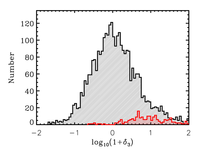 Figure 12.— The distribution of overdensity measures for all sources with
a secure redshift at in the joint population comprised
of the ACES redshift catalog and the set of existing public
redshifts detailed in §2. The red histogram shows
the environment distribution for the galaxies identified as
group members using the X-ray group catalog of Finoguenov et al. (2011). There is good agreement between the group and environment
catalogs.
Table 3 ACES Environment Catalog
Figure 12.— The distribution of overdensity measures for all sources with
a secure redshift at in the joint population comprised
of the ACES redshift catalog and the set of existing public
redshifts detailed in §2. The red histogram shows
the environment distribution for the galaxies identified as
group members using the X-ray group catalog of Finoguenov et al. (2011). There is good agreement between the group and environment
catalogs.
Table 3 ACES Environment Catalog6. Summary and Future Work
We present a spectroscopic survey of the Chandra Deep Field South (CDFS), conducted using Magellan/IMACS and aptly named the Arizona CDFS Environment Survey (ACES). The survey dataset includes unique spectroscopic targets, yielding secure redshifts, within the extended CDFS region. We describe in detail the design and implementation of the survey and present preliminary redshift and environment catalogs. While this work marks a significant increase in both the spatial coverage and the sampling density of the spectroscopic observations in the CDFS, there remains much analysis of the ACES data to be completed in the future. In particular, work is presently underway to produce a relative throughput correction for the spectra, using observations of F stars that were targeted on many of the IMACS slitmasks. The F stars were observed with the same instrumental set-up as the science targets (i.e., same slitwidth, slitlength, etc.) and were included on multiple slitmasks, such that the spectra fell on each of the IMACS CCDs, allowing chip-to-chip variations in the throughput to be estimated. As discussed in §2, fainter targets () were observed on multiple (–) slitmasks, with the goal of accumulating longer integration times. In the future, these data spanning different slitmasks will be combined, which will likely improve the survey’s redshift success rate at fainter magnitudes. In parallel to this work, efforts to improve the spectral reduction procedures are currently underway, which should likewise improve the redshift completeness at all magnitudes. Likewise, future work will include extracting spectra and measuring redshifts for serendipitous detections of objects, an effort that could be helped greatly by the addition of data from different slitmasks. The completion of this ongoing work is expected to coincide with a final data release, including updated redshift and environment catalogs as well as all of the reduced IMACS spectra. Finally, analysis is underway to utilize the ACES data to study the correlations between star-formation history, morphology, and environment at , using the rich multiwavelength data in the CDFS and the increased sample size to improve upon previous efforts (e.g., Elbaz et al., 2007; Capak et al., 2007; Cooper et al., 2008b, 2010a).References
- Adami et al. (2005) Adami, C. et al. 2005, A&A, 443, 805
- Balestra et al. (2010) Balestra, I. et al. 2010, A&A, 512, A12+
- Barger et al. (2008) Barger, A. J., Cowie, L. L., & Wang, W. 2008, ApJ, 689, 687
- Capak et al. (2007) Capak, P. et al. 2007, ApJS, 172, 284
- Cardamone et al. (2010) Cardamone, C. N. et al. 2010, ApJS, 189, 270
- Cohen et al. (2000) Cohen, J. G., Hogg, D. W., Blandford, R., Cowie, L. L., Hu, E., Songaila, A., Shopbell, P., & Richberg, K. 2000, ApJ, 538, 29
- Coil et al. (2011) Coil, A. L. et al. 2011, ApJ, 741, 8
- Cooper et al. (2010a) Cooper, M. C., Gallazzi, A., Newman, J. A., & Yan, R. 2010a, MNRAS, 402, 1942
- Cooper et al. (2012a) Cooper, M. C., Newman, J. A., Davis, M., Finkbeiner, D. P., & Gerke, B. F. 2012a, in Astrophysics Source Code Library, record ascl:1203.003, 3003
- Cooper et al. (2005) Cooper, M. C., Newman, J. A., Madgwick, D. S., Gerke, B. F., Yan, R., & Davis, M. 2005, ApJ, 634, 833
- Cooper et al. (2009) Cooper, M. C., Newman, J. A., & Yan, R. 2009, ApJ, 704, 687
- Cooper et al. (2008a) Cooper, M. C., Tremonti, C. A., Newman, J. A., & Zabludoff, A. I. 2008a, MNRAS, 390, 245
- Cooper et al. (2006) Cooper, M. C. et al. 2006, MNRAS, 370, 198
- Cooper et al. (2007) —. 2007, MNRAS, 376, 1445
- Cooper et al. (2008b) —. 2008b, MNRAS, 383, 1058
- Cooper et al. (2010b) —. 2010b, MNRAS, 409, 337
- Cooper et al. (2011) —. 2011, ApJS, 193, 14
- Cooper et al. (2012b) —. 2012b, MNRAS, 419, 3018
- Cowie et al. (2004) Cowie, L. L., Barger, A. J., Hu, E. M., Capak, P., & Songaila, A. 2004, AJ, 127, 3137
- Damen et al. (2011) Damen, M. et al. 2011, ApJ, 727, 1
- Davis et al. (2003) Davis, M. et al. 2003, in Society of Photo-Optical Instrumentation Engineers (SPIE) Conference Series, Vol. 4834, Society of Photo-Optical Instrumentation Engineers (SPIE) Conference Series, ed. P. Guhathakurta, 161–172
- Davis et al. (2007) Davis, M. et al. 2007, ApJ, 660, L1
- Dawson et al. (2001) Dawson, S., Stern, D., Bunker, A. J., Spinrad, H., & Dey, A. 2001, AJ, 122, 598
- Dickinson et al. (2004) Dickinson, M. et al. 2004, ApJ, 600, L99
- Doherty et al. (2005) Doherty, M., Bunker, A. J., Ellis, R. S., & McCarthy, P. J. 2005, MNRAS, 361, 525
- Dressler et al. (2011) Dressler, A. et al. 2011, PASP, 123, 288
- Elbaz et al. (2007) Elbaz, D. et al. 2007, A&A, 468, 33
- Finoguenov et al. (2001) Finoguenov, A., Reiprich, T. H., & Böhringer, H. 2001, A&A, 368, 749
- Gawiser et al. (2006) Gawiser, E. et al. 2006, ApJS, 162, 1
- Giacconi et al. (2001) Giacconi, R. et al. 2001, ApJ, 551, 624
- Giacconi et al. (2002) —. 2002, ApJS, 139, 369
- Giavalisco et al. (2004) Giavalisco, M. et al. 2004, ApJ, 600, L93
- Gilli et al. (2003) Gilli, R. et al. 2003, ApJ, 592, 721
- Gladders & Yee (2005) Gladders, M. D. & Yee, H. K. C. 2005, ApJS, 157, 1
- Grogin et al. (2011) Grogin, N. A. et al. 2011, ApJS, 197, 35
- Kaiser (1987) Kaiser, N. 1987, MNRAS, 227, 1
- Kirby et al. (2007) Kirby, E. N., Guhathakurta, P., Faber, S. M., Koo, D. C., Weiner, B. J., & Cooper, M. C. 2007, ApJ, 660, 62
- Koekemoer et al. (2011) Koekemoer, A. M. et al. 2011, ApJS, 197, 36
- Le Fèvre et al. (2004) Le Fèvre, O. et al. 2004, A&A, 428, 1043
- Lehmer et al. (2005) Lehmer, B. D. et al. 2005, ApJS, 161, 21
- Lowenthal et al. (1997) Lowenthal, J. D. et al. 1997, ApJ, 481, 673
- Magnelli et al. (2009) Magnelli, B., Elbaz, D., Chary, R. R., Dickinson, M., Le Borgne, D., Frayer, D. T., & Willmer, C. N. A. 2009, A&A, 496, 57
- Magnelli et al. (2011) —. 2011, A&A, 528, A35+
- Mignoli et al. (2005) Mignoli, M. et al. 2005, A&A, 437, 883
- Miller et al. (2008) Miller, N. A., Fomalont, E. B., Kellermann, K. I., Mainieri, V., Norman, C., Padovani, P., Rosati, P., & Tozzi, P. 2008, ApJS, 179, 114
- Newman et al. (2012) Newman, J. A. et al. 2012, ArXiv:1203.3192
- Oke & Gunn (1983) Oke, J. B. & Gunn, J. E. 1983, ApJ, 266, 713
- Padovani et al. (2009) Padovani, P., Mainieri, V., Tozzi, P., Kellermann, K. I., Fomalont, E. B., Miller, N., Rosati, P., & Shaver, P. 2009, ApJ, 694, 235
- Phillips et al. (1997) Phillips, A. C., Guzman, R., Gallego, J., Koo, D. C., Lowenthal, J. D., Vogt, N. P., Faber, S. M., & Illingworth, G. D. 1997, ApJ, 489, 543
- Popesso et al. (2009) Popesso, P. et al. 2009, A&A, 494, 443
- Quadri et al. (2007) Quadri, R. et al. 2007, AJ, 134, 1103
- Ravikumar et al. (2007) Ravikumar, C. D. et al. 2007, A&A, 465, 1099
- Reddy et al. (2006) Reddy, N. A., Steidel, C. C., Erb, D. K., Shapley, A. E., & Pettini, M. 2006, ApJ, 653, 1004
- Rix et al. (2004) Rix, H.-W. et al. 2004, ApJS, 152, 163
- Roche et al. (2006) Roche, N. D., Dunlop, J., Caputi, K. I., McLure, R., Willott, C. J., & Crampton, D. 2006, MNRAS, 370, 74
- Salimbeni et al. (2009) Salimbeni, S. et al. 2009, A&A, 501, 865
- Silverman et al. (2010) Silverman, J. D. et al. 2010, ApJS, 191, 124
- Szokoly et al. (2004) Szokoly, G. P. et al. 2004, ApJS, 155, 271
- Treu et al. (2005) Treu, T. et al. 2005, ApJ, 633, 174
- Trevese et al. (2007) Trevese, D., Castellano, M., Fontana, A., & Giallongo, E. 2007, A&A, 463, 853
- Vanzella et al. (2005) Vanzella, E. et al. 2005, A&A, 434, 53
- Vanzella et al. (2006) —. 2006, A&A, 454, 423
- Vanzella et al. (2008) —. 2008, A&A, 478, 83
- Vanzella et al. (2009) —. 2009, ApJ, 695, 1163
- Weiner et al. (2006) Weiner, B. J. et al. 2006, ApJ, 653, 1049
- Willmer et al. (2006) Willmer, C. N. A. et al. 2006, ApJ, 647, 853
- Wirth et al. (2004) Wirth, G. D. et al. 2004, AJ, 127, 3121
- Wolf et al. (2001) Wolf, C., Dye, S., Kleinheinrich, M., Meisenheimer, K., Rix, H.-W., & Wisotzki, L. 2001, A&A, 377, 442
- Wolf et al. (2008) Wolf, C., Hildebrandt, H., Taylor, E. N., & Meisenheimer, K. 2008, A&A, 492, 933
- Wolf et al. (2004) Wolf, C. et al. 2004, A&A, 421, 913
- Xue et al. (2011) Xue, Y. Q. et al. 2011, ApJS, 195, 10
Abstract
We present the Arizona CDFS Environment Survey (ACES), a recently-completed spectroscopic redshift survey of the Chandra Deep Field South (CDFS) conducted using IMACS on the Magellan-Baade telescope. In total, the survey targeted unique sources down to a limiting magnitude of , yielding secure redshifts across the extended CDFS region. The ACES dataset delivers a significant increase to both the spatial coverage and the sampling density of the spectroscopic observations in the field. Combined with previously-published, spectroscopic redshifts, ACES now creates a highly-complete survey of the galaxy population at , enabling the local galaxy density (or environment) on relatively small scales ( Mpc) to be measured at in one of the most heavily-studied and data-rich fields in the sky. Here, we describe the motivation, design, and implementation of the survey and present a preliminary redshift and environment catalog. In addition, we utilize the ACES spectroscopic redshift catalog to assess the quality of photometric redshifts from both the COMBO-17 and MUSYC imaging surveys of the CDFS.