Towards precise calculation of transport coefficients in the hadron gas. The shear and the bulk viscosities.

Abstract

The shear and the bulk viscosities of the hadron gas at low temperatures are studied in the model with constant elastic cross sections being relativistic generalization of the hard spheres model. One effective radius ${r=0.4~{}fm}$ is chosen for all elastic collisions. Only elastic collisions are considered which are supposed to be dominant at temperatures ${T\leq 120-140~{}MeV}$. The calculations are done in the framework of the Boltzmann equation with the Boltzmann statistics distribution functions and the ideal gas equation of state. The applicability of these approximations is discussed. It’s found that the bulk viscosity of the hadron gas is much larger than the bulk viscosity of the pion gas while the shear viscosity is found to be less sensitive to the mass spectrum of hadrons. The constant cross sections and the Boltzmann statistics approximation allows one not only to conduct precise numerical calculations of transport coefficients in the hadron gas but also to obtain some relatively simple relativistic analytical closed-form expressions. Namely, the correct single-component first-order shear viscosity coefficient is found. The single-component first-order nonequilibrium distribution function, some analytical results for the binary mixture and expressions for mean collision rates, mean free paths and times are presented. Comparison with some previous calculations for the hadron gas and the pion gas is done too. This paper is the first step towards calculations with inelastic processes included.

I Introduction

The bulk and the shear viscosity coefficients are transport coefficients which enter in hydrodynamical equations and thus are important for studying of nonequilibrium evolution of any thermodynamic system.

Although experimental value of the shear viscosity was found to be small in the hadron gas smalleta , lacey there are two more additional reasons to study the shear viscosity. The first one is the experimentally observed minimum of the ratio of the shear viscosity to the entropy density $\eta/s$ near the liquid-gas phase transition for different substances which may help in studying of the quantum chromodynamics phase diagram and finding of the location of the critical point Csernai:2006zz , lacey . For a counterexample see arXiv:1010.3119 and references therein. The second reason is calculation of the $\eta/s$ in strongly interacting systems, preferably real ones, for testing of the conjectured lowest bound $\eta/s=\frac{1}{4\pi}$ adscftbound , found in some conformal field theories having dual gravity theories, and search of a new one. The bound $\eta/s=\frac{1}{4\pi}$ was violated with different counterexamples. For some reasonable ones see Buchel:2008vz , Sinha:2009ev . Also see the recent review arXiv:1108.0677 . The bulk viscosity may be not negligibly small and is expected to have a maximum near the phase transition Kharzeev:2007wb , Karsch:2007jc , chakkap .

Whether one uses the Kubo formula or the Boltzmann equation one faces nearly the same integral equation for transport coefficients jeon , jeonyaffe , Arnold:2002zm . The preferable way to solve it is the variational (or Ritz) method. Due to its complexity often the relaxation time approximation is used in the framework of the Boltzmann equation. Though this approximation is inaccurate, does not allow to control precision of approximation and can potentially lead to large deviations. The main difficulty in the variational method is in calculation of collision integrals. To calculate any transport coefficient in the lowest approximation in a mixture like the hadron gas with very large number of components $N^{\prime}$ one would need to calculate roughly ${N^{\prime}}^{2}$ special 12-dimensional integrals if only elastic collisions are considered. Fortunately it’s possible to simplify these integrals considerably and perform these calculations in reasonable time.

This paper contains calculations of the shear and the bulk viscosity coefficients for the hadron-resonance gas in the constant elastic differential cross sections model. The calculations are done in the framework of the Boltzmann equation with classical Boltzmann statistics, without medium effects and with the ideal gas equation of state. The constant cross sections and the Boltzmann statistics approximation allows one to obtain some relatively simple analytical closed-form expressions.

The numerical calculations for the hadron-resonance gas presented in this paper are the first step towards calculations with number-changing (inelastic) processes taken into account. Then, possibly, more realistic model of strong interactions and quantum statistics will be implemented. These calculations can be considered as quite precise at low temperatures where elastic collisions dominate and equation of state is close to the ideal gas equation of state.

The main applications of the results of this paper are to hydrodynamical description of heavy ion collisions, like in Fogaca:2013cma . See also the review of such applications Kapusta:2008vb . Though, analytical results of the present paper can be applied to other fields of physics, like cosmology, see, e. g., BasteroGil:2012zr . There are also other ways of dissipative description, which can be mentioned, see, e. g. dissipcoef .

For comparison calculations for the pion gas are performed and the results are found to be close to the results in prakash where only elastic processes were considered and the ideal gas equation of state was used or to the results in davesne (at zero chemical potential) where the Bose statistics was used instead of the Boltzmann one. The comparison is shown in fig. 1. The discrepancies arise because of the constant cross sections approximation used in this paper. Smaller values of the viscosities in prakash for some temperature range originate because of the $\rho$-resonance contribution to the quasielastic $\pi\pi$ cross section and the maximum of the bulk viscosity is expected to be shifted towards lower temperatures. In these calculations the nonvanishing value of the bulk viscosity is obtained only due to the mass of pions.

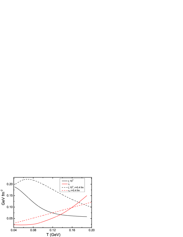
Figure 1: Dashed lines designate calculations for the pion gas performed in the constant cross sections approximation with the hard core radius $r=0.4~{}fm$. The solid black line designates the 3-rd order bulk viscosity and the solid red line designates the 1-st order shear viscosity of the pion gas from prakash , where the quasielastic (with contribution of the $\rho$-resonance) semi-empirical $\pi\pi$ cross section was used.

In several papers the bulk viscosity $\xi$ was calculated for the pion gas using the chiral perturbation theory and some other approaches with quite large discrepancies between quantitative results. In fernnicola calculations were done by the Kubo formula in rough approximation. There the number-changing ${2\leftrightarrow 4}$ processes were neglected too and the non-vanishing value of the bulk viscosity is obtained due to trace anomaly and the mass of pions. At small temperatures where effects of trace anomaly are small the magnitude of the bulk viscosity is large in compare to the results of this paper and prakash , davesne . For example, at ${T=60~{}MeV}$ the bulk viscosity is roughly 20 times more. The calculations in lumoore are done in the framework of the Boltzmann equation and have divergent dependence of the $\xi(T)$ for ${T\rightarrow 0}$ because of weak ${2\leftrightarrow 4}$ number-changing processes taken into account and at ${T=140~{}MeV}$ the bulk viscosity is nearly 44 times larger than the bulk viscosity calculated in this paper. Though calculations in lumoore were done in the first order approximation which does not even take into account elastic collisions so that this discrepancy can become smaller few times after more accurate calculations. The function $\xi(T)$ may turn out to be not smooth at the middle temperatures and the smooth function $\xi(T)$ is to be obtained through extrapolation. In dobado the bulk viscosity was calculated in the framework of the Boltzmann equation with the ideal gas equation of state and only elastic collisions taken into account. The Inverse Amplitude Method was used to get the scattering amplitudes of pions. The quantitative results are close to the results in prakash ; davesne . Calculations in the paper chenwang are done in the framework of the Boltzmann equation for massless pions. There the bulk viscosity increases rapidly so that the ratio $\xi/s$ increases with the temperature.

Calculation of the shear viscosity in the hadron gas, done in Gorenstein:2007mw using some approximate formula and in toneev using relaxation time approximation, are in good agreement with calculations in this paper. The bulk viscosity of the hadron gas, calculated in toneev has similar dependence on the temperature though it is roughly 10-30 times more than the bulk viscosity calculated in this paper. At low temperature ${T=100~{}MeV}$ and vanishing chemical potentials it is 20 times more. In nhngr calculation of the bulk viscosity was done for the hadron-resonance gas with masses less than $2~{}GeV$ using some special formula obtained though an ansatz for the small frequency limit of the spectral density at zero spatial momentum Kharzeev:2007wb . There the bulk viscosity to entropy density ratio $\xi/s$ has similar behavior to the $\xi/s$ in this paper and is roughly 2 times more.

The bulk and the shear viscosities were calculated in the linear $\sigma$-model with number-changing processes taken into account and nonideal gas equation of state chakkap . This model has chiral symmetry restoration phase transition and can qualitatively describe pion gas. These calculations demonstrate example that the ratio of the shear viscosity to the entropy density $\eta/s$ has the minimum near the phase transition and the ratio of the bulk viscosity to the entropy density $\xi/s$ can have a maximum near the phase transition for some values of the vacuum sigma mass if the peak in the $\xi$ is sharp enough.

The structure of the paper is the following. Sec. II contains the constant cross sections model description. The applicability of the used approximations is discussed in Sec. III. The Boltzmann equation, its solution and general form of the transport coefficients can be found in Sec. IV. The numerical calculations for the hadron gas are presented in Sec. V. In Sec. VI.1 analytical results for the single-component gas are presented. In particular analytical expression for the first order single-component shear viscosity coefficient, found before in anderson , is corrected while the bulk viscosity coefficient remains the same. Also the nonequilibrium distribution function in the same approximation is written. Some analytical results for the binary mixture are considered in Sec. VI.2. Integrals of source terms needed for calculation of the transport coefficients can be found in Appendix A. The general entropy density formula used in numerical calculations for the hadron gas can be found in Appendix B. Transformations of the collision brackets being the 12-dimensional integrals which enter in transport coefficients can be found in Appendix C. The closed-form expressions for collision rates, mean free paths and mean free times are included in Appendix D.

II The hard core interaction model

In non-relativistic classical theory of particle interactions there is a widespread model called the hard core repulsion model or model of hard spheres with some radius $r$. For applications for the high-energy nuclear collisions see Gorenstein:2007mw and references therein. The differential scattering cross section for this model can be inferred from the problem of scattering of point particle on the spherical potential ${U(r)=\infty}$ if ${r\leq a}$ and ${U(r)=0}$ if ${r>a}$ landau1 . In this model the differential cross section is equal to $a^{2}/4$. To apply this result to the gas of hard spheres with radius $r$ one can notice that the scattering of two spheres can be considered as the scattering of the point particle on the sphere of the radius $2r$, so that one should take ${a=2r}$. The full cross section is obtained after integration over angles of the $r^{2}d\Omega$ which results in the $4\pi r^{2}$. For collisions of hard spheres of different radiuses one should take ${a=r_{1}+r_{2}}$ or replace $r$ on $\frac{r_{1}+r_{2}}{2}$. The relativistic generalization of this model is the constant (not dependent on the scattering energy and angle) differential cross sections model.

The hard spheres model is classical and connection of its cross sections to cross sections calculated in any quantum theory is needed. For particles having spin the differential cross sections averaged over the initial spin states and summed over the final ones will be used. If colliding particles are identical and their differential cross section is integrated over the momentums (or the spatial angle to get the total cross section) then it should be multiplied on the factor $\frac{1}{2}$ to cancel double counting of the momentum states. These factors are exactly the factors $\gamma_{kl}$ next to the collision integrals in the Boltzmann equations (22). The differential cross sections times these factors will be called the classical differential cross sections.

From the analysis of semi-empirical total elastic cross sections in prakash for $\pi\pi$, $\pi K$, $\pi N$, $KN$ and $NN$ collisions one can find that the elastic part without resonance contribution of the total cross sections lies approximately in the range ${10-30~{}mb=1-3~{}fm^{2}}$ (except for $NN$ cross section reaching $50~{}mb$ for small energies). From comparison of these values with the total cross sections in the hard spheres model one finds for the radius ${r=0.28-0.49~{}fm}$. For simplification the mean value is chosen equal to ${r=0.4~{}fm}$ in numerical calculations for all hadron and resonance elastic cross sections. Then classical differential cross sections become equal to some one constant value too. In this approximation the cross section will enter in the transport coefficients as one factor.

III Conditions of applicability

First the applicability of the Boltzmann equation and of calculations of transport coefficients should be clarified.

Although the Boltzmann equation is valid for any perturbations of the distribution function it should be a slowly varying function of space-time coordinate to justify that it can be considered as a function of macroscopic quantities like temperature, chemical potential or flow velocity or in other words that one can apply thermodynamics locally. Then one can make expansion over independent gradients of thermodynamic functions and flow velocity (the Chapman-Enskog method), which vanish in equilibrium. Smallness of these perturbations of the distribution functions in compare to theirs main parts ensures the validity of this expansion and that the gradients are small. Because these perturbations are inversely proportional to coupling constants one can say that they are proportional to some product of particles’ mean free paths and the gradients. So that in other words the mean free paths should be much smaller than the characteristic lengths on which macroscopic quantities change considerably.

The system with number-changing processes should be treated additionally. Number-changing processes are very important for the bulk viscosity. If the coupling constant of inelastic number-changing processes is small then the bulk viscosity is dominated by the inelastic processes jeon . Formally tending coupling constants of inelastic processes to zero the bulk viscosity diverges together with the nonequilibrium perturbations of the distribution functions, which should be small. Though this dependence can become invalid earlier if inelastic processes are negligible in some sense, because the limiting case with completely switched off inelastic processes can be well defined. That’s why there is a need to specify reasonable conditions when inelastic processes can be neglected. Some simple ones of them are proposed below. It is smallness of the time $t$ on which the system’s evolution is considered in compare to the mean free time for number-changing processes of the $k^{\prime}$-th particle species, $t^{inel}_{k^{\prime}}$ (221),

$$\frac{t}{t^{inel}_{k^{\prime}}}=tR^{inel}_{k^{\prime}}\ll 1,$$ (1)

where $R^{inel}_{k^{\prime}}$ is the rate of inelastic processes per particle of the $k^{\prime}$-th species. Similar condition, stating that the number of reactions is smaller than unity, can be used:

$$tV\sum_{n\in~{}\text{all channels}}\widetilde{R}^{inel}_{k^{\prime},n}<1,$$ (2)

where $V$ is the system’s volume and $\sum_{n\in~{}\text{all channels}}\widetilde{R}^{inel}_{k^{\prime},n}$ is the number of the inelastic reactions of particles of the $k^{\prime}$-th species over all channels per unit time per unit volume. Though in mixtures with mean free times of inelastic processes close to each other one might need to use relevant sums of reaction rates instead of reaction rates for certain species. Also one can consider natural time-scales like relaxation times of the gradients or thermodynamic functions. Estimations of the thermal and chemical relaxation times for pions were done in Song:1996ik . Basing on these results one can expect that the approximate temperature where inelastic processes cease to be efficient is ${T=120-140~{}MeV}$ for vanishing chemical potentials. For nonzero chemical potentials this temperature is expected to be smaller.

Errors due to the Boltzmann statistics used instead of the Bose or the Fermi ones were found to be small for vanishing chemical potentials. According to calculations for the pion gas in davesne the bulk viscosity becomes $25\%$ larger at ${T=120~{}MeV}$ and $33\%$ larger at ${T=200~{}MeV}$ for vanishing chemical potential. Although the relative deviations of the thermodynamic quantities of the pion gas at nonvanishing chemical potential ${\mu=100~{}MeV}$ are not more than $20\%$ the bulk viscosity becomes up to $2.5$ times more. The shear viscosity becomes $15\%$ less at ${T=120~{}MeV}$ and $25\%$ less at ${T=200~{}MeV}$ for vanishing chemical potential and $33\%$ less at ${T=120~{}MeV}$ and $67\%$ less at ${T=200~{}MeV}$ for the ${\mu=100~{}MeV}$. The corrections to the bulk viscosity of the fermion gas, according to calculations of the bulk viscosity source term not presented in this paper, are of the opposite sign and approximately of the same magnitude.

The condition of applicability of the ideal gas equation of state is controlled by the dimensionless parameter $\upsilon n$ which appears in the first correction from the binary collisions in the virial expansion and should be small. Here ${\upsilon=16\pi r^{3}/3}$ is the so called excluded volume parameter and $1/n$ is the mean volume per particle. One finds ${\upsilon n\approx 0.09}$ at ${T=120~{}MeV}$ and ${\upsilon n\approx 0.2}$ at ${T=140~{}MeV}$ for vanishing chemical potentials. Though even small corrections to thermodynamic quantities can result in large corrections for the bulk viscosity as it was found for the quantum statistics corrections. Along the freeze-out line (its parameters can be found in Gorenstein:2007mw ) the $\upsilon n$ grows from $0.07$ to $0.49$ with the temperature.

One more important requirement which one needs to justify the Boltzmann equation approach is that the mean free time should be much larger than $\hbar/\Omega$ ($\Omega$ is the characteristic single-particle energy) danielewicz or de Broglie wavelength should be much smaller than the mean free path Arnold:2002zm to distinguish independent acts of collisions and for particles to have well-defined on-shell energy and momentum. This condition gets badly satisfied for high temperatures or densities. The mean free path of particle species $k^{\prime}$ is given by the formula (222) or the formula (217) if inelastic processes can be neglected. The wavelength can be written as ${\lambda_{k^{\prime}}=\frac{1}{\langle\left|\vec{p}_{k^{\prime}}\right|\rangle}}$, where the averaged modulus of momentum of $k^{\prime}$-th species $\langle\left|\vec{p}_{k^{\prime}}\right|\rangle$ is

$$\langle\left|\vec{p}_{k^{\prime}}\right|\rangle=\frac{\int d^{3}p_{k^{\prime}}|\vec{p}_{k^{\prime}}|f^{(0)}_{k^{\prime}}(p_{k^{\prime}})}{\int d^{3}p_{k^{\prime}}f^{(0)}_{k^{\prime}}(p_{k^{\prime}})}=\frac{2e^{-z_{k^{\prime}}}T(3+3z_{k^{\prime}}+z_{k^{\prime}}^{2})}{z_{k^{\prime}}^{2}K_{2}(z_{k^{\prime}})}=\sqrt{\frac{8m_{k^{\prime}}T}{\pi}}\frac{K_{5/2}(z_{k^{\prime}})}{K_{2}(z_{k^{\prime}})},$$ (3)

where ${z_{k^{\prime}}\equiv m_{k^{\prime}}/T}$, $K_{2}(x)$ is the modified Bessel function of the second kind. As it follows from the (3) the largest wavelength is for the lightest particles, $\pi$-mesons. The elastic collision mean free paths are close to each other for all particle species. Hence, the smallest value of the ratio $\lambda_{k^{\prime}}/l^{el}_{k^{\prime}}$ is for $\pi$-mesons. Its value is close to the value of the $\upsilon n$ and is exponentially suppressed for small temperatures too. At temperature ${T=140~{}MeV}$ and vanishing chemical potentials this ratio is equal to $0.18$. Along the freeze-out line it grows from $0.12$ to $0.37$ with the temperature.

If the last requirement is not satisfied one can use the Kubo formulas, for instance. In jeon it was shown that intermediate integral equations for the shear and the bulk viscosities coming after linearization of the Boltzmann equation and expansion over gradients of the flow velocity can be reproduced from the Kubo formulas in scalar ${g\phi^{3}+\lambda\phi^{4}}$ theory. The difference is in that one has to replace particles’ masses with temperature dependent ones and to use thermal matrix elements for elastic and inelastic collisions. Basing on this result an example of effective kinetic theory of quasiparticle excitations valid for all temperatures was presented in jeonyaffe . For further developments see Arnold:2002zm , Gagnon:2006hi , Gagnon:2007qt . For other approaches see Blaizot:1992gn , Calzetta:1986cq , Calzetta:1999ps and Arnold:1997gh with references therein.

IV Details of calculations

IV.1 The Boltzmann equation and its solution

Calculations in this paper go close to the ones in groot though with some differences and generalizations. Let’s start from some definitions. Multi-indices $k,l,m,n$ will be used to denote particle species with certain spin states. Indexes $k^{\prime},l^{\prime},m^{\prime},n^{\prime}$ will be used to denote particle species without regard to their spin states (and run from 1 to the number of particle species $N^{\prime}$) and $a,b$ to denote conserved quantum numbers. Because nothing depends on spin variables one has for every sum over the multi-indexes

$$\sum_{k}...=\sum_{k^{\prime}}g_{k^{\prime}}...,$$ (4)

where $g_{k^{\prime}}$ is the spin degeneracy factor. The following assignments will be used

$$n\equiv\sum_{k}n_{k} \equiv \sum_{k^{\prime}}n_{k^{\prime}},\quad n_{a}\equiv\sum_{k}q_{ak}n_{k},\quad x_{k}\equiv\frac{n_{k}}{n},\quad x_{k^{\prime}}\equiv\frac{n_{k^{\prime}}}{n},\quad x_{a}\equiv\frac{n_{a}}{n},$$

$$\hat{\mu}_{k} = \frac{\mu_{k}}{T},\quad\hat{\mu}_{a}=\frac{\mu_{a}}{T},\quad z_{k}\equiv\frac{m_{k}}{T},\quad\pi_{k}^{\mu}\equiv\frac{p_{k}^{\mu}}{T},\quad\tau_{k}\equiv\frac{p_{k}^{\mu}U_{\mu}}{T},$$ (5)

where $q_{ak}$ denotes values of conserved quantum numbers of the $a$-th kind of the $k$-th particle species. Everywhere the particle number densities are summed the spin degeneracy factor $g_{k^{\prime}}$ appears and then gets absorbed into the $n_{k^{\prime}}$ or the $x_{k^{\prime}}$ by definition. All other quantities with primed and unprimed indexes don’t differ, except for rates, mean free times and mean free paths defined in Appendix D, the $\gamma_{kl}$ commented below, the coefficients $A_{k^{\prime}l^{\prime}}^{rs}$, $C_{k^{\prime}l^{\prime}}^{rs}$ and, of course, quantities whose free indexes set indexes of the particle number densities $n_{k}$. Also the assignment ${\int\frac{d^{3}p_{k}}{p_{k}^{0}}\equiv\int_{p_{k}}}$ will be used somewhere for compactness.

The particle number flows are

$$N^{\mu}_{k}=\int\frac{d^{3}p_{k}}{(2\pi)^{3}p^{0}_{k}}p^{\mu}_{k}f_{k},$$ (6)

where the assignment ${f_{k}(p_{k})\equiv f_{k}}$ is introduced. The energy-momentum tensor is

$$T^{\mu\nu}=\sum_{k}\int\frac{d^{3}p_{k}}{(2\pi)^{3}p_{k}^{0}}p_{k}^{\mu}p_{k}^{\nu}f_{k}.$$ (7)

The local equilibrium distribution functions are

$$f^{(0)}_{k}=e^{(\mu_{k}-p_{k}^{\mu}U_{\mu})/T},$$ (8)

where $\mu_{k}$ is the chemical potential of the $k$-th particle species, $T$ is the temperature and $U_{\mu}$ is the relativistic flow 4-velocity such that ${U_{\mu}U^{\mu}=1}$ (with frequently used consequence ${U_{\mu}\partial_{\nu}U^{\mu}=0}$). The local equilibrium is considered as perturbations of independent thermodynamic variables and the flow velocity over a global equilibrium such that they can depend on the space-time coordinate $x^{\mu}$. Though such perturbations are not the general ones and do not take into account all possible deviations from a chemical equilibrium. For numerical calculations along the freeze-out line, where such deviations are important, saturation $\gamma$-factors are used, see Cleymans:2005xv , Andronic:2005yp and references therein. The chemical equilibrium implies that the particle number densities are equal to their global equilibrium values. The global equilibrium is called the time-independent stationary state with the maximal entropy. The global equilibrium of isolated system can be found by variation of the total nonequilibrium entropy functional landau5 over the distribution function with condition of the total energy and the total net charges conservation:

$$U[f]=\sum_{k}\int\frac{d^{3}p_{k}d^{3}x}{(2\pi)^{3}}f_{k}(1-\ln f_{k})-\sum_{k}\int\frac{d^{3}p_{k}d^{3}x}{(2\pi)^{3}}\beta p^{0}_{k}f_{k}-\sum_{a,k}\lambda_{a}q_{ak}\int\frac{d^{3}p_{k}d^{3}x}{(2\pi)^{3}}f_{k},$$ (9)

where $\beta,\lambda_{a}$ are Lagrange coefficients. Equating the first variation to zero one easily gets the function (8) with ${U^{\mu}=(1,0,0,0)}$, ${\beta=\frac{1}{T}}$ and

$$\mu_{k}=\sum_{a}q_{ak}\mu_{a},$$ (10)

where ${\mu_{a}=\lambda_{a}}$ are the independent chemical potentials coupled to conserved net charges.

With ${f_{k}=f_{k}^{(0)}}$ substituted in the (6) and the (7) one gets the leading contribution in the gradients expansion of the particle number flow and the energy-momentum tensor

$$N^{(0)\mu}_{k}=n_{k}U^{\mu},$$ (11)

$$T^{(0)\mu\nu}=\epsilon U^{\mu}U^{\nu}-P\Delta^{\mu\nu},$$ (12)

where the projector

$$\Delta^{\mu\nu}\equiv g^{\mu\nu}-U^{\mu}U^{\nu},$$ (13)

is introduced. The $n_{k}$ is the ideal gas particle number density

$$n_{k}=U_{\mu}N^{(0)\mu}_{k}=\frac{1}{2\pi^{2}}T^{3}z_{k}^{2}K_{2}(z_{k})e^{\hat{\mu}_{k}},$$ (14)

the $\epsilon$ is the ideal gas energy density

$$\epsilon=U_{\mu}U_{\nu}T^{(0)\mu\nu}=\sum_{k}\int\frac{d^{3}p_{k}}{(2\pi)^{3}}p_{k}^{0}f_{k}^{(0)}=\sum_{k}n_{k}e_{k},\quad e_{k}\equiv m_{k}\frac{K_{3}(z_{k})}{K_{2}(z_{k})}-T,$$ (15)

and the $P$ is the ideal gas pressure

$$P=-\frac{1}{3}T^{(0)\mu\nu}\Delta_{\mu\nu}=\sum_{k}\frac{1}{3}\int\frac{d^{3}p_{k}}{(2\pi)^{3}p_{k}^{0}}\vec{p_{k}}^{2}f_{k}^{(0)}=\sum_{k}n_{k}T=nT.$$ (16)

Also the following assignments are used

$$e \equiv \frac{\epsilon}{n}=\sum_{k}x_{k}e_{k},\quad h_{k}\equiv e_{k}+T,\quad h\equiv\frac{\epsilon+P}{n}=\sum_{k}x_{k}h_{k},$$

$$\hat{e}_{k} \equiv \frac{e_{k}}{T}=z_{k}\frac{K_{3}(z_{k})}{K_{2}(z_{k})}-1,\quad\hat{e}\equiv\frac{e}{T},\quad\hat{h}_{k}\equiv\frac{h_{k}}{T}=z_{k}\frac{K_{3}(z_{k})}{K_{2}(z_{k})},\quad\hat{h}\equiv\frac{h}{T}.$$ (17)

Above $h$ is the enthalpy per particle, $e$ is the energy per particle and $h_{k}$, $e_{k}$ are the enthalpy and the energy per particle of the $k$-th particle species correspondingly which are well defined in the ideal gas.

In relativistic hydrodynamics the flow velocity $U^{\mu}$ needs some extended definition in relation to the thermodynamic quantities. The most convenient condition applied to $U^{\mu}$ is the Landau-Lifshitz condition landau6 . This condition states that in the local rest frame (where the flow velocity is zero though its gradient can have nonzero value) each fluid cell should have zero momentum and its energy and net charge densities should be related to other thermodynamic quantities through the equilibrium thermodynamic relations (without contribution of nonequilibrium dissipations). Its covariant mathematical formulation is

$$(T^{\mu\nu}-T^{(0)\mu\nu})U_{\mu}=0,\quad(N^{\mu}_{a}-N^{(0)\mu}_{a})U_{\mu}=0.$$ (18)

The next to leading correction over the gradients expansion to the $T^{\mu\nu}$ can be written as expansion over the 1-st order Lorentz covariant gradients which are rotationally and space inversion invariant and satisfy the Landau-Lifshitz condition (18):

$$T^{(1)\mu\nu}\equiv 2\eta\overset{\circ}{\overline{\nabla^{\mu}U^{\nu}}}+\xi\Delta^{\mu\nu}\nabla_{\rho}U^{\rho}=\eta\left(\Delta^{\mu}_{\rho}\Delta^{\nu}_{\tau}+\Delta^{\nu}_{\rho}\Delta^{\mu}_{\tau}-\frac{2}{3}\Delta^{\mu\nu}\Delta_{\rho\tau}\right)\nabla^{\rho}U^{\tau}+\xi\Delta^{\mu\nu}\nabla_{\rho}U^{\rho},$$ (19)

where for any tensor $a_{\mu\nu}$ the symmetrized traceless tensor assignment is introduced

$$\overset{\circ}{\overline{a_{\mu\nu}}}\equiv\left(\frac{\Delta_{\mu\rho}\Delta_{\nu\tau}+\Delta_{\nu\rho}\Delta_{\mu\tau}}{2}-\frac{1}{3}\Delta_{\mu\nu}\Delta_{\rho\tau}\right)a^{\rho\tau}\equiv\Delta_{\mu\nu\rho\tau}a^{\rho\tau},\quad\Delta^{\mu\nu}_{~{}~{}\rho\tau}\Delta^{\rho\tau}_{~{}~{}\sigma\lambda}=\Delta^{\mu\nu}_{~{}~{}\sigma\lambda}.$$ (20)

The equation (19) is the definition of the shear $\eta$ and the bulk $\xi$ viscosity coefficients. The $\xi\Delta^{\mu\nu}\nabla_{\rho}U^{\rho}$ term in the (19) can be considered as nonequilibrium contribution to the pressure which enters in the (12).

By means of the projector (13) one can split the space-time derivative $\partial_{\mu}$ as

$$\partial_{\mu}=U_{\mu}U^{\nu}\partial_{\nu}+\Delta_{\mu}^{\nu}\partial_{\nu}\equiv U_{\mu}D+\nabla_{\mu}.$$ (21)

where $D\equiv U^{\nu}\partial_{\nu}$, $\nabla_{\mu}\equiv\Delta_{\mu}^{\nu}\partial_{\nu}$. In the local rest frame (where ${U^{\mu}=(1,0,0,0)}$) the $D$ becomes the time derivative and the $\nabla_{\mu}$ becomes the spacial derivative. Then the Boltzmann equations can be written in the form

$$p_{k}^{\mu}\partial_{\mu}f_{k}=(p_{k}^{\mu}U_{\mu}D+p_{k}^{\mu}\nabla_{\mu})f_{k}=C_{k}^{el}[f_{k}]+C_{k}^{inel}[f_{k}],$$ (22)

where $C_{k}^{inel}[f_{k}]$ represents the inelastic or number-changing collision integrals (it is dropped in calculations in this paper if the opposite is not stated explicitly) and $C_{k}^{el}[f_{k}]$ is the elastic ${2\leftrightarrow 2}$ collision integral. The collision integral $C_{k}^{el}[f_{k}]$ has the form of the sum of positive gain terms and negative loss terms. Its explicit form is (cf. jeon ; Arnold:2002zm )

$$C_{k}^{el}[f_{k}] = \sum_{l}\gamma_{kl}\frac{1}{2}\int\frac{d^{3}p_{1l}}{(2\pi)^{3}2p_{1l}^{0}}\frac{d^{3}p^{\prime}_{k}}{(2\pi)^{3}2{p^{\prime}}_{k}^{0}}\frac{d^{3}p^{\prime}_{1l}}{(2\pi)^{3}2{p^{\prime}}_{1l}^{0}}(f^{\prime}_{k}f^{\prime}_{1l}-f_{k}f_{1l})$$ (23)

$$\times |\mathcal{M}_{kl}|^{2}(2\pi)^{4}\delta^{4}(p^{\prime}_{k}+p^{\prime}_{1l}-p_{k}-p_{1l})$$

where ${\gamma_{kl}=\frac{1}{2}}$ if $k$ and $l$ denote the same particle species without regard to spin states and ${\gamma_{kl}=1}$ otherwise, ${|\mathcal{M}_{kl}(p^{\prime}_{k},p^{\prime}_{1l};p_{k},p_{1l})|^{2}\equiv|\mathcal{M}_{kl}|^{2}}$ is the square of dimensionless elastic scattering amplitude, averaged over the initial spin states and summed over the final ones. Index $1$ designates that $p_{k}$ and $p_{1k}$ are different variables. Introducing ${W_{kl}\equiv W_{kl}(p^{\prime}_{k},p^{\prime}_{1l};p_{k},p_{1l})}$ as

$$W_{kl}=\frac{|\mathcal{M}_{kl}|^{2}}{64\pi^{2}}\delta^{4}(p^{\prime}_{k}+p^{\prime}_{1l}-p_{k}-p_{1l}),$$ (24)

one can rewrite the collision integral (23) in the form as in groot

$$C_{k}^{el}[f_{k}]=(2\pi)^{3}\sum_{l}\gamma_{kl}\int_{p_{1l},{p^{\prime}}_{k},{p^{\prime}}_{1l}}\left(\frac{f^{\prime}_{k}}{(2\pi)^{3}}\frac{f^{\prime}_{1l}}{(2\pi)^{3}}-\frac{f_{k}}{(2\pi)^{3}}\frac{f_{1l}}{(2\pi)^{3}}\right)W_{kl}.$$ (25)

The $W_{kl}$ is related to the elastic differential cross section $\sigma_{kl}$ as groot

$$W_{kl}=s\sigma_{kl}\delta^{4}(p^{\prime}_{k}+p^{\prime}_{1l}-p_{k}-p_{1l}),$$ (26)

where ${s=(p_{k}+p_{1l})^{2}}$ is the usual Mandelstam variable. The $W_{kl}$ has properties $W_{kl}(p^{\prime}_{k},p^{\prime}_{1l};p_{k},p_{1l})=W_{kl}(p_{k},p_{1l};p^{\prime}_{k},p^{\prime}_{1l})=W_{lk}(p^{\prime}_{1l},p^{\prime}_{k};p_{1l},p_{k})$ (due to time reversibility and a freedom of relabelling of order numbers of particles taking part in reaction). And e.g. $W_{kl}(p^{\prime}_{k},p^{\prime}_{1l};p_{k},p_{1l})\neq W_{kl}(p^{\prime}_{1l},p^{\prime}_{k};p_{1l},p_{k})$ in general case. Elastic collision integrals have important properties which one can easily prove groot :

$$\int\frac{d^{3}p_{k}}{(2\pi)^{3}p^{0}_{k}}C_{k}^{el}[f_{k}]=0,$$ (27)

$$\sum_{k}\int\frac{d^{3}p_{k}}{(2\pi)^{3}p^{0}_{k}}p_{k}C_{k}^{el}[f_{k}]=0.$$ (28)

Also the $C^{el}_{k}[f_{k}]$ vanishes if ${f_{k}=f^{(0)}_{k}}$.

The distribution functions $f_{k}$ solving the system of the Boltzmann equations approximately are sought in the form

$$f_{k}=f^{(0)}_{k}+f^{(1)}_{k}\equiv f^{(0)}_{k}+f^{(0)}_{k}\varphi_{k}(x,p_{k}),$$ (29)

where it’s assumed that $f_{k}$ depend on the $x^{\mu}$ entirely through the $T$, $\mu_{k}$, $U^{\mu}$ or their space-time derivatives. Also it is assumed that ${|\varphi_{k}|\ll 1}$. After substitution of ${f_{k}=f^{(0)}_{k}}$ in the (22) the r.h.s. becomes zero and the l.h.s. is zero only if the $T$, $\mu_{k}$ and $U^{\mu}$ don’t depend on the $x^{\mu}$ (provided they don’t depend on the momentum $p^{\mu}_{k}$). The 1-st order space-time derivatives of the $T$, $\mu_{k}$, $U^{\mu}$ in the l.h.s. should be cancelled by the first nonvanishing contribution in the r.h.s. This means that the $\varphi_{k}$ should be proportional to the 1-st order space-time derivatives of the $T$, $\mu_{k}$, $U^{\mu}$. The covariant time derivatives $D$ can be expressed through the covariant spacial derivatives by means of approximate hydrodynamical equations, valid at the same order in the gradients expansion. Let’s derive them. Integrating the (22) over the $\frac{d^{3}p_{k}}{(2\pi)^{3}p^{0}_{k}}$ with the ${f_{k}=f^{(0)}_{k}}$ in the l.h.s. with inelastic collision integrals retained and using the (27) and the (6) one would get (which can be justified with explicit form of inelastic collision integrals)

$$\partial_{\mu}N^{(0)\mu}_{k}=Dn_{k}+n_{k}\nabla_{\mu}U^{\mu}=I_{k},$$ (30)

where $I_{k}$ is the sum of inelastic collision integrals integrated over momentum. It is responsible for nonconservation of the total particle number of the $k$-th particle species and has property ${\sum_{k}q_{ak}I_{k}=0}$. If ${C^{inel}_{k}[f_{k}]=0}$ then ${I_{k}=0}$ which results in conservation of the total particle numbers of each particle species. Multiplying the (30) on the $q_{ak}$ and summing over $k$ one gets the continuity equations for the net charge flows:

$$\partial_{\mu}N^{(0)\mu}_{a}=Dn_{a}+n_{a}\nabla_{\mu}U^{\mu}=0.$$ (31)

Then integrating the (22) over the $p_{k}^{\mu}\frac{d^{3}p_{k}}{(2\pi)^{3}p^{0}_{k}}$ with the ${f_{k}=f^{(0)}_{k}}$ in the l.h.s. one gets

$$\partial_{\rho}T^{(0)\rho\nu}=\partial_{\rho}(\epsilon U^{\rho}U^{\nu}-P\Delta^{\rho\nu})=0.$$ (32)

There is zero in the r.h.s. even if inelastic collision integrals are retained because they respect energy conservation too. Note that the Boltzmann equations (22) permit self-consistent consideration only of the ideal gas energy-momentum tensor and net charge flows. After convolution of the (32) with the $\Delta^{\mu}_{\nu}$ one gets the Euler’s equation

$$DU^{\mu}=\frac{1}{\epsilon+P}\nabla^{\mu}P=\frac{1}{hn}\nabla^{\mu}P.$$ (33)

After convolution of the (32) with the $U_{\nu}$ one gets equation for the energy density

$$D\epsilon=-(\epsilon+P)\nabla_{\mu}U^{\mu}=-hn\nabla_{\mu}U^{\mu}.$$ (34)

To proceed further one needs to expand the l.h.s. of the Boltzmann equations (22) over the gradients of thermodynamic variables and the flow velocity. Let’s choose $\mu_{a}$ and $T$ as independent thermodynamic variables. Then for the $Df^{(0)}_{k}$ one can write expansion

$$Df^{(0)}_{k}=\sum_{a}\frac{\partial f^{(0)}_{k}}{\partial\mu_{a}}D\mu_{a}+\frac{\partial f^{(0)}_{k}}{\partial T}DT+\frac{\partial f^{(0)}_{k}}{\partial U^{\mu}}DU^{\mu}.$$ (35)

Writing the expansion for the $Dn_{a}$ and the $D\epsilon$ one gets from the (31) and the (34):

$$Dn_{a}=\sum_{b}\frac{\partial n_{a}}{\partial\mu_{b}}D\mu_{b}+\frac{\partial n_{a}}{\partial T}DT=-n_{a}\nabla_{\mu}U^{\mu},$$ (36)

$$D\epsilon=\frac{\partial\epsilon}{\partial T}DT+\sum_{a}\frac{\partial\epsilon}{\partial\mu_{a}}D\mu_{a}=-hn\nabla_{\mu}U^{\mu}.$$ (37)

The solution to the system of equations (36), (37) can easily be found:

$$DT=-RT\nabla_{\mu}U^{\mu},$$ (38)

$$D\mu_{a}=T\sum_{b}\tilde{A}^{-1}_{ab}(RB_{b}-x_{b})\nabla_{\mu}U^{\mu},$$ (39)

where

$$R\equiv\frac{\hat{h}-\sum_{a,b}E_{a}\tilde{A}^{-1}_{ab}x_{b}}{C_{\{\mu\}}-\sum_{a,b}E_{a}\tilde{A}^{-1}_{ab}B_{b}},$$ (40)

and

$$\frac{\partial n_{a}}{\partial\mu_{b}}\equiv\frac{n}{T}\tilde{A}_{ab},\quad\frac{\partial n_{a}}{\partial T}\equiv\frac{n}{T}B_{a},\quad\frac{\partial\epsilon}{\partial T}\equiv nC_{\{\mu\}},\quad\frac{\partial\epsilon}{\partial\mu_{a}}\equiv nE_{a}.$$ (41)

Above it is assumed that the matrix $\tilde{A}_{ab}$ is not degenerate, which is the case usually. Otherwise uncertainties or singularities from $D\mu_{a}$ enter in the bulk viscosity. Using the ideal gas formulas (14) and (15) one gets

$$\tilde{A}_{ab} = \sum_{k}q_{ak}q_{bk}x_{k},\quad E_{a}=\sum_{k}q_{ak}x_{k}\hat{e}_{k},\quad B_{a}=E_{a}-\sum_{b}\tilde{A}_{ab}\hat{\mu}_{b},$$

$$C_{\{\mu\}} = \sum_{k}x_{k}(3\hat{h}_{k}+z_{k}^{2}-\hat{\mu}_{k}\hat{e}_{k})=\sum_{k}x_{k}(3\hat{h}_{k}+z_{k}^{2})-\sum_{a}E_{a}\hat{\mu}_{a}.$$ (42)

From the (IV.1) one can see that the matrix $\tilde{A}_{ab}$ has positive diagonal elements and in the case of one kind of charge it’s always not degenerate. For the special case of vanishing chemical potentials, $\mu_{a}=0$, the quantities $n_{a}$, $x_{a}$, $B_{a}$, $E_{a}$ tend to zero because the contributions from particles and anti-particles cancel each other and chargeless particles don’t contribute. Then from the (38) and the (39) one finds

$$DT|_{\mu_{a}=0}=-\frac{h}{C_{\{\mu\}}}\nabla_{\mu}U^{\mu},$$ (43)

$$D\mu_{a}|_{\mu_{a}=0}=0.$$ (44)

This means that for vanishing chemical potentials one can simply exclude them from the distribution functions (if one does not study diffusion and thermal conductivity). In systems with only elastic collisions each particle has its own charge so that one takes ${q_{ak}=\delta_{ak}}$ and gets

$$\tilde{A}_{kl} = \delta_{kl}x_{k},\quad B_{k}=x_{k}(\hat{e}_{k}-\hat{\mu}_{k}),\quad E_{k}=\hat{e}_{k}x_{k},\quad R=\frac{1}{c_{\upsilon}}$$

$$C_{\{\mu\}} - \sum_{a,b}E_{a}\tilde{A}^{-1}_{ab}B_{b}=\sum_{k}x_{k}(-\hat{h}_{k}^{2}+5\hat{h}_{k}+z_{k}^{2}-1)\equiv\sum_{k}x_{k}c_{\upsilon,k}\equiv c_{\upsilon}.$$ (45)

Then the equation for the $DT$ (38) remains the same with a new $R$ from the (IV.1) and the equations (39) become:

$$D\mu_{k}=\left(\frac{T}{c_{\upsilon}}(\hat{e}_{k}-\hat{\mu}_{k})-T\right)\nabla_{\mu}U^{\mu}.$$ (46)

Note that in systems with only elastic collisions the $D\mu_{k}$ does not tend to zero for vanishing chemical potentials so that the $\mu_{k}$ could not be omitted in the distribution functions in this case. Because the heat conductivity and diffusion are not considered in this paper their nonequilibrium gradients are taken equal to zero, $\nabla_{\nu}P=\nabla_{\nu}T=\nabla_{\nu}\mu_{a}=0$. Using the (38), (39) and (33) the l.h.s. of the (22) can be transformed as

$$(p_{k}^{\mu}U_{\mu}D+p_{k}^{\mu}\nabla_{\mu})f_{k}^{(0)}=-Tf_{k}^{(0)}\pi_{k}^{\mu}\pi_{k}^{\nu}\overset{\circ}{\overline{\nabla_{\mu}U_{\nu}}}+Tf_{k}^{(0)}\hat{Q}_{k}\nabla_{\rho}U^{\rho},$$ (47)

where

$$\hat{Q}_{k}\equiv\tau_{k}^{2}\left(\frac{1}{3}-R\right)+\tau_{k}\left[\sum_{a,b}q_{ak}\tilde{A}^{-1}_{ab}(RB_{b}-x_{b})+\hat{\mu}_{k}R\right]-\frac{1}{3}z_{k}^{2}.$$ (48)

Using the (20) one can notice that the useful equality ${\pi_{k}^{\mu}\pi_{k}^{\nu}\overset{\circ}{\overline{\nabla_{\mu}U_{\nu}}}=\overset{\circ}{\overline{\pi_{k}^{\mu}\pi_{k}^{\nu}}}\overset{\circ}{\overline{\nabla_{\mu}U_{\nu}}}}$ holds. In systems with only elastic collisions the $\hat{Q}_{k}$ simplifies in agreement with groot :

$$\hat{Q}_{k}=\left(\frac{4}{3}-\gamma\right)\tau_{k}^{2}+\tau_{k}((\gamma-1)\hat{h}_{k}-\gamma)-\frac{1}{3}z_{k}^{2}.$$ (49)

where the assignments $\gamma$ from groot is used. It can be expressed through the $c_{\upsilon}$, defined in the (IV.1), as ${\gamma\equiv\frac{1}{c_{\upsilon}}+1}$. Introducing symmetric round brackets

$$(F,G)_{k}\equiv\frac{1}{4\pi z_{k}^{2}K_{2}(z_{k})T^{2}}\int_{p_{k}}F(p_{k})G(p_{k})e^{-\tau_{k}}.$$ (50)

and assignments

$$\alpha_{k}^{r}\equiv(\hat{Q}_{k},(\tau_{k})^{r}),\quad\gamma_{k}^{r}\equiv((\tau_{k})^{r}\overset{\circ}{\overline{\pi_{k}^{\mu}\pi_{k}^{\nu}}},\overset{\circ}{\overline{\pi_{k\mu}\pi_{k\nu}}}),\quad a^{r}_{k}\equiv(1,(\tau_{k})^{r})_{k},$$ (51)

and using explicit expressions of the $a_{k}^{r}$ from Appendix A one finds for the $\alpha_{k}^{0}$ and the $\alpha_{k}^{1}$ in systems with elastic and inelastic collisions:

$$\alpha_{k}^{0}=1+\sum_{a,b}q_{ak}\tilde{A}^{-1}_{ab}(RB_{b}-x_{b})-(\hat{e}_{k}-\hat{\mu}_{k})R,$$ (52)

$$\alpha_{k}^{1}=\hat{h}_{k}+\sum_{a,b}\hat{e}_{k}q_{ak}\tilde{A}^{-1}_{ab}(RB_{b}-x_{b})-(3\hat{h}_{k}+z_{k}^{2}+\hat{\mu}_{k}(1-\hat{h}_{k}))R.$$ (53)

Then using the (52) and the (53) one can show that

$$\sum_{k}q_{ak}x_{k}\alpha_{k}^{0}=0,$$ (54)

$$\sum_{k}x_{k}\alpha_{k}^{1}=0.$$ (55)

Because the gradients $\nabla_{\mu}U^{\mu}$ and $\overset{\circ}{\overline{\nabla_{\mu}U_{\nu}}}$ are independent the (54) and the (55) are direct consequences of the local net charge (31) and the energy-momentum (32) conservations. Quantities $(1,\overset{\circ}{\overline{\pi^{\mu}_{k}\pi^{\nu}_{k}}})$ and $(p_{k}^{\lambda},\overset{\circ}{\overline{\pi^{\mu}_{k}\pi^{\nu}_{k}}})$ vanish automatically because of the special tensorial structure of the $\overset{\circ}{\overline{\pi^{\mu}_{k}\pi^{\nu}_{k}}}$.

The next step is to transform the r.h.s of the Boltzmann equations (22). After substitution of the (29) in the r.h.s. of the (22) the collision integral becomes linear and one gets

$$C_{k}^{el}[f_{k}]\approx-f_{k}^{(0)}\sum_{l}\mathcal{L}_{kl}^{el}[\varphi_{k}],$$ (56)

where

$$\mathcal{L}_{kl}^{el}[\varphi_{k}]\equiv\frac{\gamma_{kl}}{(2\pi)^{3}}\int_{p_{1l},{p^{\prime}}_{k},{p^{\prime}}_{1l}}f_{1l}^{(0)}(\varphi_{k}+\varphi_{1l}-\varphi^{\prime}_{k}-\varphi^{\prime}_{1l})W_{kl},$$ (57)

The unknown function $\varphi_{k}$ is sought in the form

$$\varphi_{k}=\frac{1}{n\sigma(T)}\left(-A_{k}(p_{k})\nabla_{\mu}U^{\mu}+C_{k}(p_{k})\overset{\circ}{\overline{\pi^{\mu}_{k}\pi^{\nu}_{k}}}\overset{\circ}{\overline{\nabla_{\mu}U_{\nu}}}\right),$$ (58)

where $\sigma(T)$ is some formal averaged cross section, used to come to dimensionless quantities. Then using the (47) and the (56) and the fact that the gradients $\nabla_{\mu}U^{\mu}$ and $\overset{\circ}{\overline{\nabla_{\mu}U_{\nu}}}$ are independent the Boltzmann equations can be written as independent integral equations:

$$\hat{Q}_{k}=\sum_{l}x_{l}L_{kl}^{el}[A_{k}],$$ (59)

$$\overset{\circ}{\overline{\pi_{k}^{\mu}\pi_{k}^{\nu}}}=\sum_{l}x_{l}L_{kl}^{el}[C_{k}\overset{\circ}{\overline{\pi_{k}^{\mu}\pi_{k}^{\nu}}}],$$ (60)

where the dimensionless collision integral is introduced

$$L_{kl}^{el}[\chi_{k}]=\frac{1}{n_{l}T\sigma(T)}\mathcal{L}_{kl}^{el}[\chi_{k}].$$ (61)

In case of present inelastic processes the l.h.s of the (59) is set by the source term (48) and the r.h.s. contains linear inelastic collision integrals. After introduction of inelastic processes the source term in the (59) becomes much larger as demonstrated in Sec. VI.1. Using the equations (39) and (38) and the ideal gas formulas (IV.1) one can check that in the zero masses limit the $\hat{Q}_{k}$ (48) tend to zero and ${D\hat{\mu}_{a}=0}$ that is the $\hat{\mu}_{a}$ don’t scale and the distribution functions become scale invariant. The source term of the shear viscosity in the (60) doesn’t depend on the presence of inelastic processes in the system and originates from the free propagation term ${\frac{\vec{p}_{k}}{p_{k}^{0}}\frac{\partial f_{k}}{\partial\vec{r}}}$ in the Boltzmann equation.

IV.2 The transport coefficients and their properties

After substitution of the $f_{k}^{(1)}$ with the $\varphi_{k}$ (58) into (7) and comparison with the (19) one finds the formula for the bulk viscosity

$$\xi=-\frac{1}{3}\frac{T}{\sigma(T)}\sum_{k}x_{k}(\Delta^{\mu\nu}\pi_{\mu,k}\pi_{\nu,k},A_{k})_{k},$$ (62)

and for the shear viscosity

$$\eta=\frac{1}{10}\frac{T}{\sigma(T)}\sum_{k}x_{k}(\overset{\circ}{\overline{\pi^{\mu}_{k}\pi^{\nu}_{k}}},C_{k}\overset{\circ}{\overline{\pi_{k\mu}\pi_{k\nu}}})_{k},$$ (63)

where the relation ${\Delta^{\mu\nu}_{~{}~{}\sigma\tau}\Delta_{\mu}^{\sigma}\Delta_{\nu}^{\tau}=5}$ is used.

In kinetics the conditions, that the nonequilibrium perturbations of distribution functions does not contribute to the net charge and the energy-momentum densities, are used as convenient choice and are called conditions of fit. They reproduce the Landau-Lifshitz condition (18). The conditions of fit for the net charge densities can be written as

$$\sum_{k}q_{ak}\int\frac{d^{3}p_{k}}{(2\pi)^{3}p_{k}^{0}}p_{k}^{\mu}U_{\mu}f_{k}^{(0)}\varphi_{k}=0,$$ (64)

and for the energy-momentum density can be written as

$$\sum_{k}\int\frac{d^{3}p_{k}}{(2\pi)^{3}p_{k}^{0}}p_{k}^{\mu}p_{k}^{\nu}U_{\nu}f_{k}^{(0)}\varphi_{k}=0.$$ (65)

For the special tensorial functions $C_{k}\overset{\circ}{\overline{\pi_{k\mu}\pi_{k\nu}}}$ in the (58) they are satisfied automatically and for the scalar functions $A_{k}$ they can be rewritten in the form (the 3-vector part of the (65) is automatically satisfied)

$$\sum_{k}q_{ak}x_{k}(\tau_{k},A_{k})_{k}=0,\quad\sum_{k}x_{k}(\tau_{k}^{2},A_{k})_{k}=0.$$ (66)

For a single-component gas with only elastic processes the conditions (64) and (65) exclude zero modes that is nonphysical solutions, proportional to the $p^{\mu}$ and a constant, for which elastic collision integral vanishes. In a single-component gas with inelastic collisions a constant is not a zero mode. For a multi-component gas these conditions would just modify the functional space on which solutions are sought. With help of these conditions of fit one can show explicitly essential positiveness of the $\xi$. Namely, using the conditions of fit (66), the equation (59) and the identity ${\Delta^{\mu\nu}\pi_{\mu,k}\pi_{\nu,k}=z_{k}^{2}-\tau_{k}^{2}}$ the bulk viscosity (62) can be rewritten as

$$\xi=\frac{T}{\sigma(T)}\sum_{k}x_{k}(\hat{Q}_{k},A_{k})_{k}=\frac{T}{\sigma(T)}\sum_{k}x_{k}\left(\sum_{l}x_{l}L^{el}_{kl}[A_{k}],A_{k}\right)_{k}=\frac{T}{\sigma(T)}[\{A\},\{A\}],$$ (67)

where the square brackets are introduced for sets of equal lengths ${\{F\}=(F_{1},...,F_{k},...)}$, ${\{G\}=(G_{1},...,G_{k},...)}$:

$$[\{F\},\{G\}]\equiv\frac{1}{n^{2}\sigma(T)}\sum_{k,l}\frac{\gamma_{kl}}{(2\pi)^{6}}\int_{p_{k},p_{1l},{p^{\prime}}_{k},{p^{\prime}}_{1l}}f^{(0)}_{k}f^{(0)}_{1l}(F_{k}+F_{1l}-{F^{\prime}}_{k}-{F^{\prime}}_{1l})G_{k}W_{kl}.$$ (68)

Using the time reversibility property of the $W_{kl}$ one can show that equality

$$(F_{k}+F_{1l}-{F^{\prime}}_{k}-{F^{\prime}}_{1l})G_{k}=\frac{1}{4}(F_{k}+F_{1l}-{F^{\prime}}_{k}-{F^{\prime}}_{1l})(G_{k}+G_{1l}-{G^{\prime}}_{k}-{G^{\prime}}_{1l}),$$ (69)

holds under integration and summation in the (68). Then one gets the direct consequence

$$[\{F\},\{G\}]=[\{G\},\{F\}],\quad[\{F\},\{F\}]\geq 0.$$ (70)

This proves the essential positiveness of the $\xi$. Similarly using the (60) the shear viscosity can be rewritten in essentially positive form

$$\eta = \frac{1}{10}\frac{T}{\sigma(T)}\sum_{k}x_{k}\left(\overset{\circ}{\overline{\pi_{k}^{\mu}\pi_{k}^{\nu}}},C_{k}\overset{\circ}{\overline{\pi_{k\mu}\pi_{k\nu}}}\right)_{k}=\frac{1}{10}\frac{T}{\sigma(T)}\sum_{k}x_{k}\left(\sum_{l}x_{l}L^{el}_{kl}[C_{k}\overset{\circ}{\overline{\pi_{k}^{\mu}\pi_{k}^{\nu}}}],C_{k}\overset{\circ}{\overline{\pi_{k\mu}\pi_{k\nu}}}\right)_{k}$$ (71)

$$= \frac{1}{10}\frac{T}{\sigma(T)}[\{C\overset{\circ}{\overline{\pi^{\mu}\pi^{\nu}}}\},\{C\overset{\circ}{\overline{\pi_{\mu}\pi_{\nu}}}\}].$$

The considered variational method allows to find approximate solution of the integral equations (59) and (60) in the form of linear combination of test-functions with coefficients, found from condition to deliver extremum to some functional, which is equivalent to solving the integral equations. One could take this functional in the form of some special norm as in groot . Or one can take somewhat different functional like in Arnold:2003zc , which is more convenient, and get the same result. This generalized functional can be written in the form

$$F[\chi]=\sum_{k}x_{k}(S_{k}^{\mu...\nu},\chi_{k\mu...\nu})_{k}-\frac{1}{2}[\{\chi_{k}^{\mu...\nu}\},\{\chi_{k\mu...\nu}\}],$$ (72)

where ${S_{k}^{\mu...\nu}=\hat{Q}_{k}}$ and ${\chi_{k\mu...\nu}=A_{k}}$ for the bulk viscosity and ${S_{k}^{\mu...\nu}=\overset{\circ}{\overline{\pi_{k}^{\mu}\pi_{k}^{\nu}}}}$, ${\chi_{k}^{\mu...\nu}=C_{k}\overset{\circ}{\overline{\pi_{k}^{\mu}\pi_{k}^{\nu}}}}$ for the shear viscosity. Equating to zero the first variance of the (72) over the $\chi_{k\mu...\nu}$ one gets

$$\sum_{k}x_{k}(S_{k}^{\mu...\nu},\delta\chi_{k\mu...\nu})_{k}-[\{\chi_{k}^{\mu...\nu}\},\{\delta\chi_{k\mu...\nu}\}]=0.$$ (73)

Because variations $\delta\chi_{k\mu...\nu}$ are arbitrary and independent the generalized integral equation follows then:

$$S_{k}^{\mu...\nu}=\sum_{l}x_{l}L^{el}_{kl}[\chi_{k\mu...\nu}].$$ (74)

The second variation of the (72) is

$$\delta^{2}F[\chi]=-[\{\delta\chi_{k}^{\mu...\nu}\},\{\delta\chi_{k\mu...\nu}\}]\leq 0,$$ (75)

which means that solution of the integral equations (59) and (60) is reduced to variational problem of finding the maximum of the functional (72). Using the (74) the maximal value of the (72) can be written as

$$F_{max}[\chi]=\frac{1}{2}[\{\chi_{k}^{\mu...\nu}\},\{\chi_{k\mu...\nu}\}]|_{\chi=\chi_{\max}}.$$ (76)

Then using the (67) and the (71) one can write the bulk and the shear viscosities through the maximal value of the $F[\chi]$

$$\xi=\left.2\frac{T}{\sigma(T)}F_{max}\right|_{S_{k}^{\mu...\nu}=\hat{Q}_{k},\,\chi_{k\mu...\nu}=A_{k}},$$ (77)

$$\eta=\left.\frac{1}{5}\frac{T}{\sigma(T)}F_{max}\right|_{S_{k}^{\mu...\nu}=\overset{\circ}{\overline{\pi_{k}^{\mu}\pi_{k}^{\nu}}},\,\chi_{k}^{\mu...\nu}=C_{k}\overset{\circ}{\overline{\pi_{k}^{\mu}\pi_{k}^{\nu}}}}.$$ (78)

This means that the precise solution of the (74) delivers the maximal values for the transport coefficients.

The approximate solution of the system of the integral equations (59) and (60) are sought in the form

$$A_{k}=\sum_{r=0}^{n_{1}}A_{k}^{r}\tau^{r}_{k},$$ (79)

$$C_{k}=\sum_{r=0}^{n_{2}}C_{k}^{r}\tau^{r}_{k},$$ (80)

where $n_{1}$ and $n_{2}$ set the number of used test-functions. Test-functions used in Arnold:2003zc would cause less significant digit cancellation in numerical calculations but there is a need to reduce the dimension of the 12-dimensional integrals from these test-functions as more as possible to perform calculations in reasonable time. The test-functions in the form of just powers of momentums seem to be the most convenient for this purpose. Questions concerning uniqueness and existence of solution and convergence of the approximate solution to the precise one are covered in groot . As long as particles of the same particle species but with different spin states are undistinguishable their functions $\varphi_{k}$ (58) are equal and the variational problem is reduced to variation of coefficients $A_{k^{\prime}}^{r}$ and $C_{k^{\prime}}^{r}$ and the bulk (67) and the shear (71) viscosities can be rewritten as

$$\xi=\frac{T}{\sigma(T)}\sum_{k^{\prime}=1}^{N^{\prime}}\sum_{r=0}^{n_{1}}x_{k^{\prime}}\alpha_{k^{\prime}}^{r}A_{k^{\prime}}^{r},$$ (81)

$$\eta=\frac{1}{10}\frac{T}{\sigma(T)}\sum_{k^{\prime}=1}^{N^{\prime}}\sum_{r=0}^{n_{2}}x_{k^{\prime}}\gamma_{k^{\prime}}^{r}C_{k^{\prime}}^{r}.$$ (82)

After substitution of the approximate functions $A_{k^{\prime}}$ (79) and $C_{k^{\prime}}$ (80) into the (72) and equating the first variation of the functional to zero one gets the following matrix equations (with multi-indexes ${(l^{\prime},s)}$ and ${(k^{\prime},r)}$) for the bulk and the shear viscosities correspondingly

$$x_{k^{\prime}}\alpha_{k^{\prime}}^{r}=\sum_{l^{\prime}=1}^{N^{\prime}}\sum_{s=0}^{n_{1}}A_{l^{\prime}k^{\prime}}^{sr}A_{l^{\prime}}^{s},$$ (83)

$$x_{k^{\prime}}\gamma_{k^{\prime}}^{r}=\sum_{l^{\prime}=1}^{N^{\prime}}\sum_{s=0}^{n_{2}}C_{l^{\prime}k^{\prime}}^{sr}C_{l^{\prime}}^{s},$$ (84)

where introduced coefficients $A_{k^{\prime}l^{\prime}}^{rs}$ and $C_{k^{\prime}l^{\prime}}^{rs}$ are

$$A_{k^{\prime}l^{\prime}}^{rs}=x_{k^{\prime}}x_{l^{\prime}}[\tau^{r},\tau_{1}^{s}]_{k^{\prime}l^{\prime}}+\delta_{k^{\prime}l^{\prime}}x_{k^{\prime}}\sum_{m^{\prime}}x_{m^{\prime}}[\tau^{r},\tau^{s}]_{k^{\prime}m^{\prime}},$$ (85)

$$C_{k^{\prime}l^{\prime}}^{rs}=x_{k^{\prime}}x_{l^{\prime}}[\tau^{r}\overset{\circ}{\overline{\pi^{\mu}\pi^{\nu}}},\tau_{1}^{s}\overset{\circ}{\overline{\pi_{1\mu}\pi_{1\nu}}}]_{k^{\prime}l^{\prime}}+\delta_{k^{\prime}l^{\prime}}x_{k^{\prime}}\sum_{m^{\prime}}x_{m^{\prime}}[\tau^{r}\overset{\circ}{\overline{\pi^{\mu}\pi^{\nu}}},\tau^{s}\overset{\circ}{\overline{\pi_{\mu}\pi_{\nu}}}]_{k^{\prime}m^{\prime}}.$$ (86)

They are expressed through the collision brackets

$$[F,G_{1}]_{kl}\equiv\frac{\gamma_{kl}}{T^{6}(4\pi)^{2}z_{k}^{2}z_{l}^{2}K_{2}(z_{k})K_{2}(z_{l})\sigma(T)}\int_{p_{k},p_{1l},{p^{\prime}}_{k},{p^{\prime}}_{1l}}e^{-\tau_{k}-\tau_{1l}}(F_{k}-{F^{\prime}}_{k})G_{1l}W_{kl}.$$ (87)

The collision brackets $[F,G]_{kl}$ are obtained from the last formula by replacement of the $G_{1l}$ on the $G_{k}$. Due to time reversibility property of the $W_{kl}$ one can replace the $G_{1l}$ on the ${\frac{1}{2}(G_{1l}-{G^{\prime}}_{1l})}$ in the (87). Then one can see that

$$[\tau^{r},\tau^{s}]_{kl}>0.$$ (88)

Also it’s easy to notice the following symmetries

$$[F,G_{1}]_{kl}=[G,F_{1}]_{lk},\quad[F,G]_{kl}=[G,F]_{kl}.$$ (89)

They result in the following symmetric properties ${A_{k^{\prime}l^{\prime}}^{rs}=A_{l^{\prime}k^{\prime}}^{sr}}$, ${C_{k^{\prime}l^{\prime}}^{rs}=C_{l^{\prime}k^{\prime}}^{sr}}$. Also the microscopical particle number and energy conservation laws imply for the $A_{l^{\prime}k^{\prime}}^{sr}$:

$$A_{k^{\prime}l^{\prime}}^{0s}=0,$$ (90)

$$\sum_{k^{\prime}}A_{k^{\prime}l^{\prime}}^{1s}=0.$$ (91)

The (90) together with the $\alpha_{k}^{0}=0$ (130) means that the equations with ${r=0}$ in the (83) are excluded. From the (91) it follows that each one equation with ${r=1}$ in the (83) can be expressed through the sum of the other ones, reducing the rank of the matrix on 1. To solve the matrix equation (83) one eliminates one equation, for example with ${k^{\prime}=1}$, ${r=1}$. One of coefficients of $A_{l^{\prime}}^{1}$ is independent, for example, let it be $A_{1^{\prime}}^{1}$. Using the (91) the matrix equation (83) can be rewritten as

$$x_{k^{\prime}}\alpha_{k^{\prime}}^{r}=\sum_{l^{\prime}=2}^{N^{\prime}}A_{l^{\prime}k^{\prime}}^{1r}(A_{l^{\prime}}^{1}-A_{1^{\prime}}^{1})+\sum_{l^{\prime}=1}^{N^{\prime}}\sum_{s=2}^{n_{1}}A_{l^{\prime}k^{\prime}}^{sr}A_{l^{\prime}}^{s}.$$ (92)

Then using the (130) and the (55) the bulk viscosity (81) becomes

$$\xi=\frac{T}{\sigma(T)}\sum_{k^{\prime}=2}^{N^{\prime}}x_{k^{\prime}}\alpha_{k^{\prime}}^{1}(A_{k^{\prime}}^{1}-A_{1^{\prime}}^{1})+\frac{T}{\sigma(T)}\sum_{k^{\prime}=1}^{N^{\prime}}\sum_{r=2}^{n_{1}}x_{k^{\prime}}\alpha_{k^{\prime}}^{r}A_{k^{\prime}}^{r}.$$ (93)

Then the coefficient $A_{1^{\prime}}^{1}$ can be eliminated by shift of other $A_{l^{\prime}}^{1}$ and be implicitly used to satisfy one energy conservation condition of fit. The particle number conservation conditions of fit are implicitly satisfied by means of the coefficients $A_{k^{\prime}}^{0}$. The first term in the (93) is present only in mixtures. That’s why it is small in gases with close to each other masses of particles of different species (like in the pion gas). In gases with very different masses (like in the hadron gas) contribution of the first term in the (93) can become dominant.

Analytical expressions for some lowest orders collision brackets which enter in the matrix equations (84) and (92) can be found in Appendix C. Higher orders are not presented because of theirs bulky form.

V The numerical calculations

The numerical calculations for the hadron gas involve roughly $2\frac{(N^{\prime}n)^{2}}{2}$ 12-dimensional integrals, where $N^{\prime}$ is the number of particle species and $n$ is the number of used test-functions (called the order of calculations). The 12-dimensional integrals being the collision brackets ${[F,G_{1}]_{kl}}$ and ${[F,G]_{kl}}$ can be reduced to 1-dimensional integrals, expressible through special functions. To compute these special functions precisely and fast they were expanded into series at several points. This allows to perform calculations at the 3-rd and the 6-th orders for the shear and the bulk viscosities correspondingly. Because analytical expressions for the collision brackets are bulky the Mathematica math was used for symbolical and some numerical manipulations. The numerical calculations are done also for temperatures above ${T=140~{}MeV}$, where inelastic collisions are expected to play important role, for future comparisons and for the bulk viscosity to show the position of its maximum in the hadron gas.

The new particle list with charmed and bottomed particles from the THERMUS package thermus is used. It comprises 508 particle species including anti-particles. These are the particles, including charmed and bottomed ones, which are more or less reliably detected Nakamura:2010zzi . It’s found that mass cut can be done on the $3~{}GeV$, which results in negligible errors ($0.01\%$ or less) in all the considered quantities. The particle list cut on the $3~{}GeV$ contains $462$ particle species including anti-particles. This list is used in calculations at zero chemical potentials (throughout the paper the chemical potentials are equal to zero if else is not stated). The results for the shear and the bulk viscosities are shown in fig. 2 and fig. 3 correspondingly. The maximal relative errors are less than $0.172\%$ for the bulk viscosity and less than $0.444\%$ for the shear viscosity. As one can see in the fig. 1 the bulk viscosity of the pion gas has maximum approximately at the temperature equal to the half of the pion’s mass. In the hadron gas this maximum shifts towards the value ${T\approx 200~{}MeV}$.

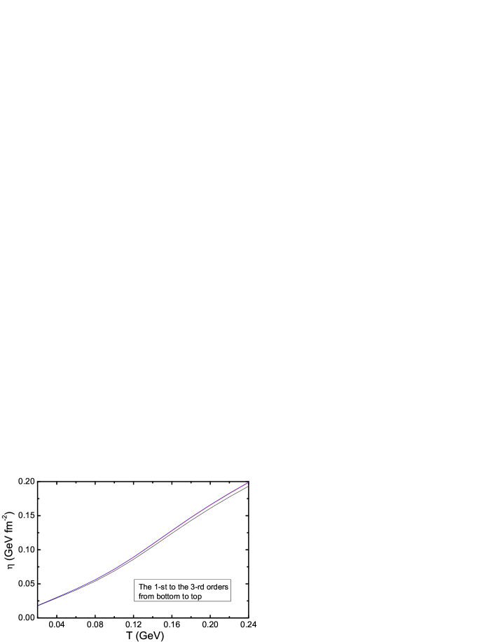
Figure 2: The shear viscosity as function of the temperature in the hadron gas calculated up to the 3-rd order. Chemical potentials are equal to zero.

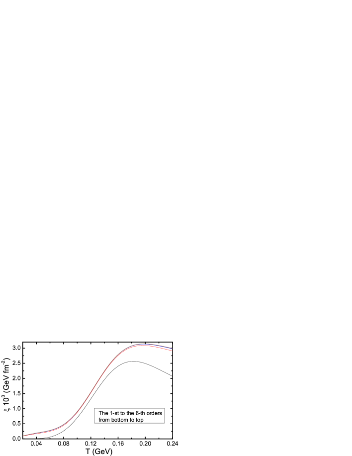
Figure 3: The bulk viscosity as function of the temperature in the hadron gas calculated up to the 6-th order. Chemical potentials are equal to zero.

The hadron gas mass spectrum dependence of transport coefficients is investigated. Particles in the list were sorted over their masses and the list was cut on the $3~{}GeV$, $2~{}GeV$, $1~{}GeV$ and on the pion’s mass. There is a separate interest to consider also hadron list with only 3 flavors. This is because, e. g., often lattice calculations are done with only 3 flavors. The 3 flavor list contains 358 particle species including anti-particles. The analogical list of the UrQMD (version 1.3) urqmd comprises 322 particle species. The deviations due to the discrepancies in these lists are no more than $0.7\%$ in the shear viscosity and no more than $2.1\%$ in the bulk viscosity, which can be ignored. Comparison of the shear viscosities calculated with different hadron lists is depicted in fig. 4. As one can see the shear viscosity changes no more than in $1.5$ times. The 3 flavor list shear viscosity is undistinguishable from the $2~{}GeV$ shear viscosity (the deviations of $0.5\%$ or smaller), so that it’s not shown. The bulk viscosity mass spectrum dependence is very strong, as depicted in fig. 5. The ratio of the bulk viscosity of the hadron gas to the bulk viscosity of the pion gas reaches $8$ at ${T=120~{}MeV}$ and $13.7$ at ${T=140~{}MeV}$. Exclusion of charmed and bottomed particles may result in even larger bulk viscosity values at some temperatures, as can be seen in the fig. 5.

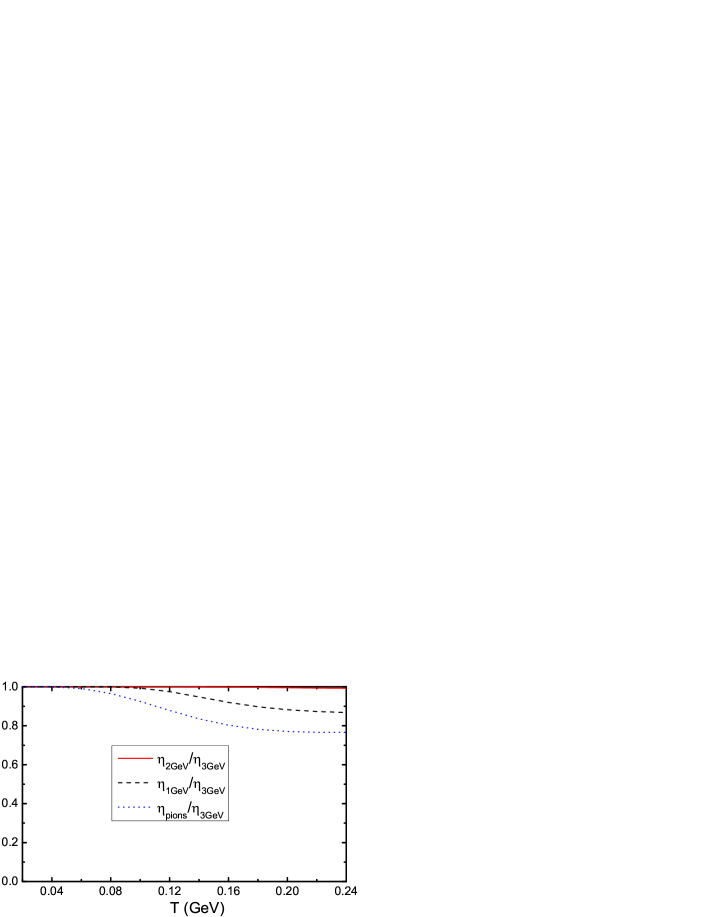
Figure 4: The ratio of the shear viscosity $\eta_{3GeV}$ with the mass spectrum cut on the $3~{}GeV$ to the shear viscosities with the mass spectrum cut on the $2~{}GeV$, $1~{}GeV$ and on the pion’s mass as functions of the temperature. Calculations are done for zero chemical potentials.

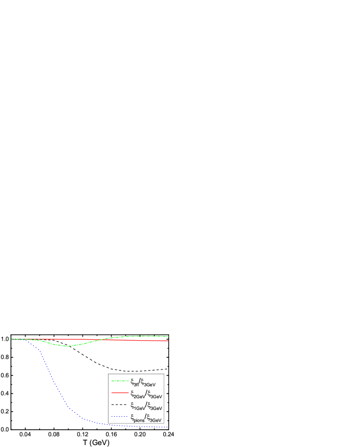
Figure 5: The ratio of the bulk viscosity $\xi_{3GeV}$ with the mass spectrum cut on the $3~{}GeV$ to the bulk viscosities with the 3 flavor hadron list, with the mass spectrum cut on the $2~{}GeV$, $1~{}GeV$ and on the pion’s mass as functions of the temperature. Calculations are done for zero chemical potentials.

The ratio of the shear viscosity to the entropy density $\eta/s$ and the ratio of the bulk viscosity to the entropy density $\xi/s$ in the hadron gas is shown in fig. 6. The ratio $\xi/s$ doesn’t have a maximum and is descending function of the temperature. The entropy density is calculated by the formula (145) using the ideal gas formulas in the (14) and the (IV.1). The ratio of the bulk viscosity to the shear viscosity is shown in fig. 7.

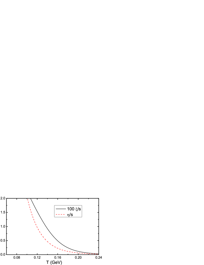
Figure 6: The ratio of the shear viscosity to the entropy density and the ratio of the bulk viscosity times 100 to the entropy density as functions of the temperature in the hadron gas. Calculations are done at zero chemical potentials.

Figure 7: The ratio of the bulk viscosity to the shear viscosity times 100 as function of the temperature in the hadron gas. Calculations are done at zero chemical potentials.

The dependence of the $\eta/s$ and the $\xi/s$ from the temperature, calculated along the freeze-out line, is found too and is depicted in fig. 8. As was discussed in Sec. III calculations with large chemical potential may contain large deviations especially for the bulk viscosity and are rather estimating. At considered collision energies strange particle numbers are not described well with the statistical model. It’s expected that this is because they doesn’t reach chemical equilibrium before the chemical freeze-out takes place. After introduction of strange saturation factors $\gamma_{s}$ experimental data gets described well Cleymans:2005xv , Andronic:2005yp . These calculations were done using the old particle list from the THERMUS package thermus (without charmed and bottomed particles, which comprise 358 particle species including anti-particles). All variables’ values of freeze-out line including the strangeness saturation factor $\gamma_{s}$ see in Gorenstein:2007mw .

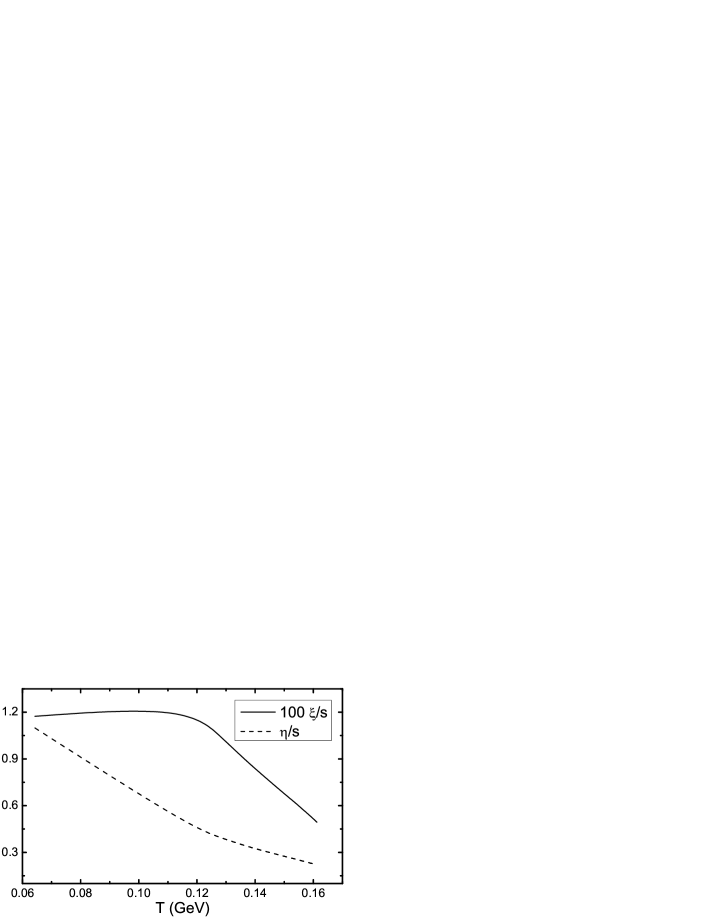
Figure 8: The shear viscosity and the bulk viscosity times 100 as functions of the freeze-out values of the temperature $T$. All other freeze-out line variables’ values can be found in Gorenstein:2007mw .

VI Analytical results

VI.1 The single-component gas

In the single-component gas with one test-function the matrix equations can be easily solved and the shear (82) and the bulk (93) viscosities become (indexes ”1” of the particle species are omitted)

$$\eta=\frac{1}{10}\frac{T}{\sigma(T)}\frac{(\gamma^{0})^{2}}{C^{00}},$$ (94)

$$\xi=\frac{T}{\sigma(T)}\frac{(\alpha^{2})^{2}}{A^{22}}.$$ (95)

In this approximation the explicit closed-form (expressed through special and elementary functions) relativistic formulas for the bulk and the shear viscosities were obtained in anderson for the model with constant cross section with the ideal gas equation of state. There the parameter ${a=2r}$. In groot they are written through the parameter ${\sigma=2r^{2}}$. The results are:

$$\eta=\frac{15}{64\pi}\frac{T}{r^{2}}\frac{z^{2}K_{2}^{2}(z)\hat{h}^{2}}{(5z^{2}+2)K_{2}(2z)+(3z^{3}+49z)K_{3}(2z)},$$ (96)

$$\xi=\frac{1}{64\pi}\frac{T}{r^{2}}\frac{z^{2}K_{2}^{2}(z)[(5-3\gamma)\hat{h}-3\gamma]^{2}}{2K_{2}(2z)+zK_{3}(2z)},$$ (97)

where ${\gamma=\frac{1}{c_{\upsilon}}+1=\frac{z^{2}+5\hat{h}-\hat{h}^{2}}{z^{2}+5\hat{h}-\hat{h}^{2}-1}}$. Though the correct result for the shear viscosity is

$$\eta=\frac{15}{64\pi}\frac{T}{r^{2}}\frac{z^{2}K_{2}^{2}(z)\hat{h}^{2}}{(15z^{2}+2)K_{2}(2z)+(3z^{3}+49z)K_{3}(2z)}.$$ (98)

This result is in agreement with the result in prakash ; leeuwen . To get the (98) and (97) the collision brackets in the $C^{00}$ (86) and $A^{22}$ (85) can be taken from Appendix C with ${z_{k}=z_{l}=z}$ and the $\gamma^{0}$ and $\alpha^{2}$ can be taken from Appendix A. In the nonrelativistic limit ${z\gg 1}$ one gets

$$\eta=\frac{5}{64\sqrt{\pi}}\frac{T}{r^{2}}\sqrt{z}\left(1+\frac{25}{16}z^{-1}+...\right),$$ (99)

$$\xi=\frac{25}{256\sqrt{\pi}}\frac{T}{r^{2}}z^{-3/2}\left(1-\frac{183}{16}z^{-1}+...\right).$$ (100)

In the ultrarelativistic limit ${z\ll 1}$ one gets

$$\eta=\frac{3}{10\pi}\frac{T}{r^{2}}\left(1+\frac{1}{20}z^{2}+...\right),$$ (101)

$$\xi=\frac{1}{288\pi}\frac{T}{r^{2}}z^{4}\left(1+\left(\frac{49}{12}-6\ln 2+6\gamma_{E}\right)z^{2}+6z^{2}\ln z+...\right).$$ (102)

where $\gamma_{E}$ is the Euler’s constant, ${\gamma_{E}\approx 0.577}$.

The perturbation of the distribution function $\varphi$ (58) can be found too:

$$\varphi=\frac{1}{n\sigma(T)}\left(-(A^{0}+A^{1}\tau+A^{2}\tau^{2})\nabla_{\mu}U^{\mu}+C^{0}\overset{\circ}{\overline{\pi^{\mu}\pi^{\nu}}}\overset{\circ}{\overline{\nabla_{\mu}U_{\nu}}}\right),$$ (103)

where the $C^{0}$ is equal to

$$C^{0}=\frac{15}{64\pi}\frac{\sigma(T)}{r^{2}}\frac{z^{2}K_{2}^{2}(z)\hat{h}}{(15z^{2}+2)K_{2}(2z)+(3z^{3}+49z)K_{3}(2z)},$$ (104)

and the $A^{2}$ is equal to

$$A^{2}=\frac{1}{64\pi}\frac{\sigma(T)}{r^{2}}\frac{z^{2}K_{2}^{2}(z)[(5-3\gamma)\hat{h}-3\gamma]}{2K_{2}(2z)+zK_{3}(2z)}.$$ (105)

The $A^{0}$ and the $A^{1}$ are used to satisfy the conditions of fit (66) and are equal to

$$A^{0}=A^{2}\frac{a^{2}a^{4}-(a^{3})^{2}}{\Delta_{A}},\quad A^{1}=A^{2}\frac{a^{2}a^{3}-a^{1}a^{4}}{\Delta_{A}},\quad\Delta_{A}\equiv a^{1}a^{3}-(a^{2})^{2},$$ (106)

where the $a^{s}$ can be found in Appendix A. In the nonrelativistic limit ${z\gg 1}$ one has

$$\varphi=\frac{5\pi e^{z-\hat{\mu}}}{32\sqrt{2}T^{3}z^{2}r^{2}}\left(-(\tau^{2}+2z\tau-z^{2})\nabla_{\mu}U^{\mu}+2\overset{\circ}{\overline{\pi^{\mu}\pi^{\nu}}}\overset{\circ}{\overline{\nabla_{\mu}U_{\nu}}}\right).$$ (107)

In the ultrarelativistic limit $z\ll 1$ one has

$$\varphi=\frac{\pi e^{-\hat{\mu}}}{480T^{3}r^{2}}\left(-5z^{2}(\tau^{2}+8\tau-12)\nabla_{\mu}U^{\mu}+36\overset{\circ}{\overline{\pi^{\mu}\pi^{\nu}}}\overset{\circ}{\overline{\nabla_{\mu}U_{\nu}}}\right).$$ (108)

Note that although the shear viscosity diverges for ${T\rightarrow\infty}$ the perturbative expansion over the gradients does not break down because the $\varphi$ does not diverge and tends to zero conversely.

The phenomenological formula, coming from the momentum transfer considerations in the kinetic-molecular theory, for the shear viscosity is ${\eta_{ph}\propto ln\langle\left|\vec{p}\right|\rangle}$ (with the coefficient of proportionality of order 1), where $\langle\left|\vec{p}\right|\rangle$ is the average relativistic momentum (3), $l$ is the mean free path. It gives correct leading $m$ and $T$ parameter dependence of the (98) with quite precise coefficient. The mean free path can be estimated as ${l\approx 1/(\sigma_{tot}n)}$ (see Appendix D). Choosing the coefficient of proportionality to match the nonrelativistic limit one gets Gorenstein:2007mw

$$\eta_{ph}=\frac{5}{64\sqrt{\pi}}\frac{\sqrt{mT}}{r^{2}}\frac{K_{5/2}(m/T)}{K_{2}(m/T)}.$$ (109)

If the bulk viscosity is expressed as ${\xi_{ph}\propto ln\langle\left|\vec{p}\right|\rangle}$ the coefficient of proportionality is not of order 1. In the nonrelativistic limit it is $25/(512\sqrt{2}z^{2})$ and in the ultrarelativistic limit it is $z^{4}/(864\pi)$. To reproduce these asymptotical dependencies the bulk viscosity should be proportional to the second power of the averaged product of the source term $\hat{Q}$ and the $\tau$ that is to the $(\alpha^{2})^{2}$.

If a system has no charges, then terms proportional to the $\tau_{k}$ in the (48) are absent, and the $R$ quantity gets another form. This results in quite different values of the $\alpha_{k}^{r}$. In particular for the single-component gas in the case ${z\gg 1}$ one gets

$$\frac{(\alpha^{2})^{2}|_{q_{11}=0}}{(\alpha^{2})^{2}|_{q_{11}=1}}=\frac{4z^{4}}{25}+...,$$ (110)

and in the case ${z\ll 1}$ one gets

$$\frac{(\alpha^{2})^{2}|_{q_{11}=0}}{(\alpha^{2})^{2}|_{q_{11}=1}}=4+....$$ (111)

In the both cases these estimates suppose enhancement of the bulk viscosity (as can be inferred from the (95)) if the number-changing processes are not negligible.

VI.2 The binary mixture

The mixture of two species with masses $m_{1}$, $m_{2}$ with different classical elastic differential constant cross sections $\sigma^{cl}_{11}$, ${\sigma^{cl}_{12}=\sigma^{cl}_{21}}$, $\sigma^{cl}_{22}$ is considered in this section. Using the (82) with ${n_{2}=0}$ and solving the matrix equation (84) one has for the shear viscosity:

$$\eta=\frac{T}{10\sigma(T)}\frac{1}{\Delta_{\eta}}[(x_{1^{\prime}}\gamma_{1}^{0})^{2}C_{2^{\prime}2^{\prime}}^{00}-2x_{1^{\prime}}x_{2^{\prime}}\gamma_{1}^{0}\gamma_{2}^{0}C_{1^{\prime}2^{\prime}}^{00}+(x_{2^{\prime}}\gamma_{2}^{0})^{2}C_{1^{\prime}1^{\prime}}^{00}],$$ (112)

where ${\Delta_{\eta}=C_{1^{\prime}1^{\prime}}^{00}C_{2^{\prime}2^{\prime}}^{00}-(C_{1^{\prime}2^{\prime}}^{00})^{2}}$. The collision brackets for the $C_{k^{\prime}l^{\prime}}^{00}$ (86) can be found in Appendix C and the $\gamma_{k}^{0}$ can be found in Appendix A.

In important limiting case when one mass is large ${z_{2}\gg 1}$ ($g_{2}$ and $\hat{\mu}_{2}$ are finite so that ${x_{2^{\prime}}\ll 1}$) and another mass is finite one can perform asymptotic expansion of special functions. Then one has ${x_{1^{\prime}}\propto O(1)}$, ${\gamma_{1}^{0}\propto O(1)}$, ${x_{2^{\prime}}\propto O(e^{-z_{2}}z_{2}^{3/2})}$, ${\gamma_{2}^{0}\propto O(z_{2})}$. Collisions of light and heavy particles dominate over collisions of heavy and heavy particles in the $C_{2^{\prime}2^{\prime}}^{00}$ and one has ${[\overset{\circ}{\overline{\pi^{\mu}\pi^{\nu}}},\overset{\circ}{\overline{\pi_{\mu}\pi_{\nu}}}]_{21}\propto O(z_{2})}$, ${C_{2^{\prime}2^{\prime}}^{00}\propto O(e^{-z_{2}}z_{2}^{5/2})}$. In the $C_{1^{\prime}1^{\prime}}^{00}$ collisions of light and light particles dominate and one gets ${C_{1^{\prime}1^{\prime}}^{00}\propto O(1)}$. And ${[\overset{\circ}{\overline{\pi^{\mu}\pi^{\nu}}},\overset{\circ}{\overline{\pi_{1\mu}\pi_{1\nu}}}]_{12}\propto O(1)}$, ${C_{1^{\prime}2^{\prime}}^{00}\propto O(e^{-z_{2}}z_{2}^{3/2})}$. In the shear viscosity the first nonvanishing contribution is the single-component shear viscosity (98), where one should take ${r^{2}=\sigma^{cl}_{11}}$ and ${z=z_{1}}$. The next correction is

$$\Delta\eta=z_{2}^{5/2}e^{-z_{2}}\frac{3Tg_{2}e^{z_{1}-\hat{\mu}_{1}+\hat{\mu}_{2}}}{64\sqrt{2\pi}(3+3z_{1}+z_{1}^{2})g_{1}\sigma^{cl}_{12}}.$$ (113)

The approximate formula Gorenstein:2007mw

$$\eta=\sum_{k}\eta_{k}x_{k},$$ (114)

where $\eta_{k}$ is given by the (98) or the (109) with mass $m_{k}$ and cross section $\sigma^{cl}_{kk}$, would give somewhat different heavy mass power dependence $O(e^{-z_{2}}z_{2}^{2})$.

Using the (93) with ${n_{1}=1}$ and solving the matrix equation (92) one has for the bulk viscosity:

$$\xi=\frac{T}{\sigma(T)}\frac{(x_{2^{\prime}}\alpha_{2}^{1})^{2}}{A_{2^{\prime}2^{\prime}}^{11}}=\frac{T}{\sigma(T)}\frac{x_{1^{\prime}}x_{2^{\prime}}\alpha_{1}^{1}\alpha_{2}^{1}}{A_{1^{\prime}2^{\prime}}^{11}}.$$ (115)

Using definition of the $A_{2^{\prime}2^{\prime}}^{11}$ (85) and the fact ${[\tau,\tau_{1}]_{kl}+[\tau,\tau]_{kl}=0}$ (179) one gets ${A_{2^{\prime}2^{\prime}}^{11}=x_{1^{\prime}}x_{2^{\prime}}[\tau,\tau]_{12}}$. Using the (88) one gets ${[\tau,\tau]_{12}>0}$. Then using ${x_{1^{\prime}}\alpha_{1}^{1}+x_{2^{\prime}}\alpha_{2}^{1}=0}$, coming from the (55), the bulk viscosity can be rewritten as

$$\xi=\frac{T}{\sigma(T)}\frac{x_{2^{\prime}}(\alpha_{2}^{1})^{2}}{x_{1^{\prime}}[\tau,\tau]_{12}}=\frac{T}{\sigma(T)}\frac{x_{1^{\prime}}(\alpha_{1}^{1})^{2}}{x_{2^{\prime}}[\tau,\tau]_{12}}>0.$$ (116)

The collision bracket $[\tau,\tau]_{12}$ can be found in Appendix C and the $\alpha_{k}^{1}$ can be found in Appendix A.

In the limiting case ${z_{2}\gg 1}$ one has ${x_{1^{\prime}}\propto O(1)}$, ${x_{2^{\prime}}\propto O(e^{-z_{2}}z_{2}^{3/2})}$, ${\alpha_{1}^{1}\propto O(e^{-z_{2}}z_{2}^{3/2})}$, ${\alpha_{2}^{1}\propto O(1)}$, ${A_{22}^{11}\propto A_{12}^{11}\propto O(e^{-z_{2}}z_{2}^{1/2})}$, ${[\tau,\tau]_{12}\propto O(z_{2}^{-1})}$. Then for the bulk viscosity one gets

$$\xi=e^{-z_{2}}z_{2}^{5/2}\frac{g_{2}Te^{-\hat{\mu}_{1}+\hat{\mu}_{2}+z_{1}}[2z_{1}^{2}-5-2\hat{h}_{1}^{2}+10\hat{h}_{1}]^{2}}{128\sqrt{2\pi}g_{1}\sigma^{cl}_{12}(z_{1}^{2}+3z_{1}+3)[z_{1}^{2}-1-\hat{h}_{1}^{2}+5\hat{h}_{1}]^{2}}+....$$ (117)

VII Concluding remarks

The shear and the bulk viscosities of the hadron gas and the pion gas were calculated at low temperatures in the model with constant cross sections. The physics of the bulk viscosity is very interesting. In particular it was found that in mixtures with only elastic collisions it can strongly depend on the mass spectrum. For instance, at temperature ${T=120~{}MeV}$ the bulk viscosity of the hadron gas is larger in 8 times than the bulk viscosity of the pion gas. Also the bulk viscosity can strongly depend on quantum statistics corrections, equation of state and inelastic processes which can be explained by nontrivial form of its source term. Inclusion of inelastic processes in pion gas at ${T=140~{}MeV}$ results in increase of the bulk viscosity roughly in 44 times according to comparison with results of the paper lumoore . It’s a future task to switch off carefully inelastic processes where they can be considered as negligible ones to perform calculation of the bulk viscosity in the pion gas and the hadron gas. The shear viscosity is less dependent on the mass spectrum and on quantum statistics corrections and its source term is some trivial function which doesn’t depend on inelastic processes.

Appendix A Values of $\alpha^{r}_{k}$, $\gamma_{k}^{r}$ and $a_{k}^{r}$

Their definitions are

$$\alpha_{k}^{r}\equiv(\hat{Q}_{k},(\tau_{k})^{r}),\quad\gamma_{k}^{r}\equiv((\tau_{k})^{r}\overset{\circ}{\overline{\pi_{k}^{\mu}\pi_{k}^{\nu}}},\overset{\circ}{\overline{\pi_{k\mu}\pi_{k\nu}}}),\quad a^{s}_{k}\equiv(1,(\tau_{k})^{s})_{k},$$ (118)

where the round brackets are

$$(F,G)_{k}\equiv\frac{1}{4\pi z_{k}^{2}K_{2}(z_{k})T^{2}}\int_{p_{k}}F(p_{k})G(p_{k})e^{-\tau_{k}}.$$ (119)

Then one can rewrite the $a_{k}^{s}$ as

$$a_{k}^{s}=\frac{1}{z_{k}^{2}K_{2}(z_{k})}\int_{z_{k}}^{\infty}d\tau(\tau^{2}-z_{k}^{2})^{1/2}\tau^{s}e^{-\tau}.$$ (120)

There is recurrence relation for the $a^{s}_{k}$:

$$a^{s}_{k}=(s+1)a^{s-1}_{k}+z_{k}^{2}a^{s-2}_{k}-(s-2)z_{k}^{2}a^{s-3}_{k}.$$ (121)

It can be derived from the (120) written in the form

$$a_{k}^{s}=\frac{1}{z_{k}^{2}K_{2}(z_{k})}\int_{z_{k}}^{\infty}d\tau(\tau^{2}-z_{k}^{2})^{3/2}\tau^{s-2}e^{-\tau}+z_{k}^{2}a_{k}^{s-2}.$$ (122)

Then after integration by parts the recurrence relation follow. Some values of the $a_{k}^{s}$ are

$$a^{0}_{k}=\frac{1}{z_{k}^{2}}(\hat{h}_{k}-4),$$ (123)

$$a^{1}_{k}=1,$$ (124)

$$a^{2}_{k}=\hat{h}_{k}-1,$$ (125)

$$a^{3}_{k}=3\hat{h}_{k}+z_{k}^{2},$$ (126)

$$a^{4}_{k}=(15+z_{k}^{2})\hat{h}_{k}+2z_{k}^{2},$$ (127)

$$a^{5}_{k}=6(15+z_{k}^{2})\hat{h}_{k}+z_{k}^{2}(15+z_{k}^{2}),$$ (128)

$$a^{6}_{k}=(630+45z_{k}^{2}+z_{k}^{4})\hat{h}_{k}+5z_{k}^{2}(21+z_{k}^{2}).$$ (129)

The $\alpha_{k}^{r}$ can be expressed through the $a^{r}_{k}$ after integration of the (48) (or the (49) if only elastic collisions are considered) over momentum and using the definition (118). For systems with only elastic collisions some values of the $\alpha_{k}^{r}$ are written below, in agreement with groot :

$$\alpha_{k}^{0}=0,$$ (130)

$$\alpha_{k}^{1}=\frac{2(c_{\upsilon}-9)\hat{h}_{k}+3\hat{h}_{k}^{2}-3z_{k}^{2}}{c_{\upsilon}}=\frac{\gamma_{k}-\gamma}{\gamma_{k}-1},$$ (131)

$$\alpha_{k}^{2}=2\hat{h}_{k}-3\frac{c_{\upsilon,k}}{c_{\upsilon}}-3\frac{\hat{h}_{k}+1}{c_{\upsilon}}=(5-3\gamma)\hat{h}_{k}-3\gamma_{k}\frac{\gamma-1}{\gamma_{k}-1},$$ (132)

where the assignments $\gamma$ and $\gamma_{k}$ from groot are used. They can be expressed through the $c_{\upsilon}$ and the $c_{\upsilon,k}$, defined in the (IV.1), as

$$\gamma\equiv\frac{1}{c_{\upsilon}}+1,\quad\gamma_{k}\equiv\frac{1}{c_{\upsilon,k}}+1.$$ (133)

The $\gamma_{k}^{r}$ can be rewritten as

$$\gamma_{k}^{r}=\frac{2}{3}\frac{1}{z_{k}^{2}K_{2}(z_{k})}\int_{z_{k}}^{\infty}d\tau(\tau^{2}-z_{k}^{2})^{5/2}\tau^{r}e^{-\tau}.$$ (134)

Then it can be rewritten through the $a_{k}^{r}$:

$$\gamma_{k}^{r}=\frac{2}{3}(a^{r+4}-2z_{k}^{2}a^{r+2}+z_{k}^{4}a^{r}).$$ (135)

Some values of the $\gamma_{k}^{r}$ are

$$\gamma_{k}^{0}=10\hat{h}_{k},$$ (136)

$$\gamma_{k}^{1}=10(6\hat{h}_{k}+z_{k}^{2}),$$ (137)

$$\gamma_{k}^{2}=10(7z_{k}^{2}+\hat{h}_{k}(42+z_{k}^{2})).$$ (138)

Appendix B The entropy density formula

The Gibbs’s potential is defined as

$$\Phi(P,T)\equiv E(S,V)-ST+PV.$$ (139)

The differential of energy is defined as

$$dE=TdS-PdV+\sum_{k}\mu_{k}dN_{k}=TdS-PdV+\sum_{a}\mu_{a}dN_{a},$$ (140)

where it is rewritten through the independent chemical potentials and the particle net charges $N_{a}$. The differential of the $\Phi$ then reads:

$$d\Phi=-SdT+VdP+\sum_{a}\mu_{a}dN_{a}.$$ (141)

Because the $\Phi$ is function of intrinsic variables $P$, $T$ and extrinsic $N_{a}$ the only possible form of it in the thermodynamic limit is

$$\Phi=\sum_{a}N_{a}\phi_{a}(P,T),$$ (142)

where $\phi_{a}$ are unknown functions. Then from the (141) one gets ${\frac{\partial\Phi}{\partial N_{a}}=\mu_{a}}$, which means that ${\phi_{a}=\mu_{a}}$. Then substituting the (142) into the (139) one gets the relation

$$\sum_{a}N_{a}\mu_{a}(P,T)=E(S,V)-ST+PV.$$ (143)

Being written for local infinitesimal volume it transforms into the expression

$$\sum_{a}n_{a}\mu_{a}=\epsilon-sT+P,$$ (144)

from where the entropy density $s$ can be found:

$$s=\frac{\epsilon+P}{T}-\sum_{a}n_{a}\hat{\mu}_{a}.$$ (145)

Appendix C Calculation of the collision brackets

The momentum parametrization and the most transformations of the 12-dimensional integrals used below are taken from groot (chap. XI and XIII). Let’s start from some assignments. The full momentum is

$$P^{\mu}\equiv p^{\mu}_{k}+p^{\mu}_{1l}={p^{\prime}}^{\mu}_{k}+{p^{\prime}}^{\mu}_{1l}.$$ (146)

The ”relative” momentums before collision $Q^{\mu}$ and after collision ${Q^{\prime}}^{\mu}$ are defined as

$$Q^{\mu}=\Delta_{P}^{\mu\nu}(p_{k\nu}-p_{1l\nu}),\quad{Q^{\prime}}^{\mu}=\Delta_{P}^{\mu\nu}({p^{\prime}}_{k\nu}-{p^{\prime}}_{1l\nu}),$$ (147)

with the assignment

$$\Delta_{P}^{\mu\nu}=g^{\mu\nu}-\frac{P^{\mu}P^{\nu}}{P^{2}},$$ (148)

where $P^{2}\equiv P^{\mu}P_{\mu}$. The covariant cosine of the scattering angle can be expressed through the $Q^{\mu}$ and the ${Q^{\prime}}^{\mu}$ as

$$\cos\Theta=-\frac{Q\cdot Q^{\prime}}{\sqrt{-Q^{2}}\sqrt{-{Q^{\prime}}^{2}}},$$ (149)

where $\cdot$ denotes convolution of 4-vectors. One also has ${Q^{2}={Q^{\prime}}^{2}}$ and

$$Q^{2}=4m_{k}^{2}-(1+\alpha_{kl})^{2}P^{2}=-\left(P^{2}-M_{kl}^{2}\right)\left[1-\frac{M_{kl}^{2}}{P^{2}}\left(1-\frac{4\mu_{kl}}{M_{kl}}\right)\right],$$ (150)

where

$$M_{kl}\equiv m_{k}+m_{l},\quad\mu_{kl}\equiv\frac{m_{k}m_{l}}{m_{k}+m_{l}},\quad\alpha_{kl}\equiv\frac{m_{k}^{2}-m_{l}^{2}}{P^{2}}=\mathrm{sign}(m_{k}-m_{l})\sqrt{1-\frac{4\mu_{kl}}{M_{kl}}}\frac{M_{kl}^{2}}{P^{2}}.$$ (151)

The function $\mathrm{sign}(x)$ is equal to 1, if ${x>0}$ and equal to $-1$, if ${x<0}$. Note that not all $P^{\mu}$ and $Q^{\mu}$ are independent:

$$P^{\mu}Q_{\mu}=0,\quad P^{\mu}{Q^{\prime}}_{\mu}=0.$$ (152)

To come from the variables ${(p_{k}^{\mu},p_{1l}^{\mu})}$ to the variables ${(P^{\mu},Q^{\mu})}$ in the measure of integration first one has to come from the ${(p_{k}^{\mu},p_{1l}^{\mu})}$ to the ${(p_{k}^{\mu}+p_{1l}^{\mu},p_{k}^{\mu}-p_{1l}^{\mu})}$ (the determinant is equal to $16$) and then shift the relative momentum $p_{k}^{\mu}-p_{1l}^{\mu}$ on the $\alpha_{kl}P^{\mu}$. Analogically for the ${({p^{\prime}}_{k}^{\mu},{p^{\prime}}_{1l}^{\mu})}$ and the ${(P^{\mu},{Q^{\prime}}^{\mu})}$. The inverse relations for the $p_{k}^{\mu},p_{1l}^{\mu},{p^{\prime}}_{k}^{\mu},{p^{\prime}}_{1l}^{\mu}$ through the $P^{\mu},Q^{\mu},{Q^{\prime}}^{\mu}$ are

$$p_{k}^{\mu}=\frac{1}{2}(1+\alpha_{kl})P^{\mu}+\frac{1}{2}{Q}^{\mu},$$ (153)

$$p_{1l}^{\mu}=\frac{1}{2}(1-\alpha_{kl})P^{\mu}-\frac{1}{2}{Q}^{\mu},$$ (154)

$${p^{\prime}}_{k}^{\mu}=\frac{1}{2}(1+\alpha_{kl})P^{\mu}+\frac{1}{2}{Q^{\prime}}^{\mu},$$ (155)

$${p^{\prime}}_{1l}^{\mu}=\frac{1}{2}(1-\alpha_{kl})P^{\mu}-\frac{1}{2}{Q^{\prime}}^{\mu}.$$ (156)

There is a need to calculate the following integrals

$$J_{kl}^{(a,b,d,e,f|q,r)}\equiv\frac{\gamma_{kl}}{T^{6}(4\pi)^{2}z_{k}^{2}z_{l}^{2}K_{2}(z_{k})K_{2}(z_{l})\sigma(T)}\int_{p_{k},p_{1l},{p^{\prime}}_{k},{p^{\prime}}_{1l}}e^{-P\cdot U/T}(1+\alpha_{kl})^{q}$$ (157)

$$\times(1-\alpha_{kl})^{r}\left(\frac{P^{2}}{T^{2}}\right)^{a}\left(\frac{P\cdot U}{T}\right)^{b}\left(\frac{Q\cdot U}{T}\right)^{d}\left(\frac{Q^{\prime}\cdot U}{T}\right)^{e}\left(\frac{-Q\cdot{Q^{\prime}}}{T^{2}}\right)^{f}W_{kl}.$$

After nontrivial transformations described in more details in groot one arrives at (the constant cross section approximation is used)

$$J_{kl}^{(a,b,d,e,f|q,r)}=\frac{\pi(d+e+1)!!\sigma^{(d,e,f)}_{1kl}}{z_{k}^{2}z_{l}^{2}K_{2}(z_{k})K_{2}(z_{l})}\sum_{q_{1}=0}^{q}\sum_{r_{1}=0}^{r}\sum_{k_{2}=0}^{\frac{d+e}{2}+f+1}\sum_{k_{3}=0}^{\frac{d+e}{2}+f+1}\sum_{h=0}^{[b/2]}(z_{k}+z_{l})^{2(q_{1}+r_{1}+k_{2}+k_{3})}$$

$$\times\left(\frac{z_{k}-z_{l}}{z_{k}+z_{l}}\right)^{q_{1}+r_{1}+2k_{3}}(-1)^{r_{1}+k_{2}+k_{3}+h}(2h-1)!!\binom{b}{2h}\binom{q}{q_{1}}\binom{r}{r_{1}}\binom{\frac{d+e}{2}+f+1}{k_{2}}$$

$$\times\binom{\frac{d+e}{2}+f+1}{k_{3}}I\left(2(a+f-q_{1}-r_{1}-k_{2}-k_{3})+3,b+\frac{d+e}{2}-h+1,z_{k}+z_{l}\right),$$

where

$$\sigma_{1kl}^{(d,e,f)}=\frac{\sigma^{cl}_{kl}}{\sigma(T)}\sum_{g=0}^{\min(d,e)}\sigma^{(f,g)}K(d,e,g),$$ (159)

where ${\sigma^{cl}_{kl}=\gamma_{kl}\sigma_{kl}}$ is the classical elastic differential constant cross section. The $\sigma^{(f,g)}$ is equal to nonzero value

$$\sigma^{(f,g)}=(2g+1)\frac{f!}{(f-g)!!(f+g+1)!!},$$ (160)

if the difference ${f-g}$ is even and ${g\leq f}$. The $K(d,e,g)$ is equal to nonzero value

$$K(d,e,g)=\frac{d!e!}{(d-g)!!(d+g+1)!!(e-g)!!(e+g+1)!!},$$ (161)

if ${g\leq\min(d,e)}$ and both ${d-g}$ and ${e-g}$ are even (which also implies that ${d+e}$ is even). The ${[...]}$ denotes the integer part. The integral $I$ is

$$I(r,n,x)\equiv x^{r+n+1}\int_{1}^{\infty}duu^{r+n}K_{n}(xu).$$ (162)

Also there is the following frequently used combination of the $J$ integrals:

$${J^{\prime}}_{kl}^{(a,b,d,e,f|q,r)}\equiv\sum_{u=0}^{f}(-1)^{u}\binom{f}{u}(2z_{k})^{2(f-u)}J_{kl}^{(a+k,b,d+e,0,0|q+2u,r)}-J_{kl}^{(a,b,d,e,f|q,r)}.$$ (163)

The first term in the difference is obtained by the replacement of the $Q^{\prime}$ on the $Q$. Using this fact the $J^{\prime}$ can be rewritten in the form

$${J^{\prime}}_{kl}^{(a,b,d,e,f|q,r)}=\frac{\pi(d+e-1)!!\sigma^{(d,e,f)}_{kl}}{z_{k}^{2}z_{l}^{2}K_{2}(z_{k})K_{2}(z_{l})}\sum_{q_{1}=0}^{q}\sum_{r_{1}=0}^{r}\sum_{k_{2}=0}^{\frac{d+e}{2}+f+1}\sum_{k_{3}=0}^{\frac{d+e}{2}+f+1}\sum_{h=0}^{[b/2]}(z_{k}+z_{l})^{2(q_{1}+r_{1}+k_{2}+k_{3})}$$

$$\times\left(\frac{z_{k}-z_{l}}{z_{k}+z_{l}}\right)^{q_{1}+r_{1}+2k_{3}}(-1)^{r_{1}+k_{2}+k_{3}+h}(2h-1)!!\binom{b}{2h}\binom{q}{q_{1}}\binom{r}{r_{1}}\binom{\frac{d+e}{2}+f+1}{k_{2}}$$

$$\times\binom{\frac{d+e}{2}+f+1}{k_{3}}I\left(2(a+f-q_{1}-r_{1}-k_{2}-k_{3})+3,b+\frac{d+e}{2}-h+1,z_{k}+z_{l}\right),$$

where

$$\sigma^{(d,e,f)}_{kl}=\frac{\sigma^{cl}_{kl}}{\sigma(T)}(d+e+1)\left(K(d+e,0,0)-\sum_{g=0}^{\min(d,e)}K(d,e,g)\sigma^{(f,g)}\right).$$ (165)

There is recurrence relation for the integral $I$ (162) groot ; luke

$$I(r,n,x)=(r-1)(r+2n-1)I(r-2,n,x)+(r-1)x^{r+n-1}K_{n}(x)+x^{r+n}K_{n+1}(x).$$ (166)

For calculations one needs only integrals $I(r,n,x)$ with positive values of the $n$ and odd values of the $r$. If ${r\geq-2n+1}$ the $I$ integrals can be expressed through the Bessel functions $K_{n}(x)$ using the (166), when ${r=1}$ or ${r=-2n+1}$. Then using the following recurrence relation for the $K_{n}(x)$ luke

$$K_{n+1}(x)=K_{n-1}(x)+\frac{2n}{x}K_{n}(x),$$ (167)

the final result can be expressed through a couple of Bessel functions. If ${r\leq-2n-1}$ then the recurrence relation (166) blows if one tries to express the $I(r,n,x)$ through the $I(-2n+1,n,x)$. Using the (166) the $I$ integrals with ${r\leq-2n-1}$ can be expressed through the integrals $G(n,x)$

$$G(n,x)\equiv I(-2n-1,n,x)=x^{-n}\int_{1}^{\infty}duu^{-n-1}K_{n}(xu).$$ (168)

There is recurrence relation for the $G(n,x)$:

$$G(n,x)=-\frac{1}{2n}(G(n-1,x)-x^{-n}K_{n}(x)).$$ (169)

It can be easily proved by integration by parts of the (168) and using the following relation for the $K_{n}(x)$ luke

$$\frac{\partial}{\partial x}K_{n}(x)=-\frac{n}{x}K_{n}(x)-K_{n-1}(x).$$ (170)

It is found that collision integrals have the simplest form if they are expressed through $G(n,x)$ with ${n=3}$ or ${n=2}$ and the Bessel functions $K_{3}(x)$ and $K_{2}(x)$ or $K_{2}(x)$ and $K_{1}(x)$. It was chosen to take ${G(x)\equiv G(3,x)}$ and $K_{3}(x)$, $K_{2}(x)$. The $G(x)$ can be expressed through the Meijer function meijer

$$G(x)=\frac{1}{32}G_{1,3}^{3,0}\left((x/2)^{2}\left|\begin{array}[]{c}1\\ -3,0,0\end{array}\right.\right).$$ (173)

The needed scalar collision brackets can be expressed through the $J^{\prime}$ as

$$[\tau^{r},\tau^{s}_{1}]_{kl}=\frac{1}{2^{r+s}}\sum_{u=1}^{r}\sum_{\upsilon=1}^{s}(-1)^{\upsilon}\binom{r}{u}\binom{s}{\upsilon}{J^{\prime}}_{kl}^{(0,r+s-u-\upsilon,u,\upsilon,0|r-u,s-\upsilon)},$$ (174)

$$[\tau^{r},\tau^{s}]_{kl}=\frac{1}{2^{r+s}}\sum_{u=1}^{r}\sum_{\upsilon=1}^{s}\binom{r}{u}\binom{s}{\upsilon}{J^{\prime}}_{kl}^{(0,r+s-u-\upsilon,u,\upsilon,0|r+s-u-\upsilon,0)},$$ (175)

and the needed tensorial collision brackets can be expressed as

$$[\tau^{r}\overset{\circ}{\overline{\pi^{\mu}\pi^{\nu}}},\tau_{1}^{s}\overset{\circ}{\overline{\pi_{1\mu}\pi_{1\nu}}}]_{kl}=\frac{1}{2^{r+s+4}}\sum_{n_{1}=0}^{r}\sum_{n_{2}=0}^{s}\binom{s}{n_{2}}\binom{r}{n_{1}}(-1)^{s-n_{2}}({J^{\prime}}_{kl}^{(2,n_{1}+n_{2},r-n_{1},s-n_{2},0|2+n_{1},2+n_{2})}$$ (176)

$$+ 2{J^{\prime}}_{kl}^{(1,n_{1}+n_{2},r-n_{1},s-n_{2},1|1+n_{1},1+n_{2})}+{J^{\prime}}_{kl}^{(0,n_{1}+n_{2},r-n_{1},s-n_{2},2|n_{1},n_{2})})$$

$$- \frac{1}{2^{r+s+3}}\sum_{n_{1}=0}^{r+1}\sum_{n_{2}=0}^{s+1}\binom{s+1}{n_{2}}\binom{r+1}{n_{1}}(-1)^{s+1-n_{2}}({J^{\prime}}_{kl}^{(1,n_{1}+n_{2},r+1-n_{1},s+1-n_{2},0|1+n_{1},1+n_{2})}$$

$$+ {J^{\prime}}_{kl}^{(0,n_{1}+n_{2},r+1-n_{1},s+1-n_{2},1|n_{1},n_{2})})+\frac{2}{3}[\tau^{r+2},\tau^{s+2}_{1}]_{kl}+\frac{1}{3}z_{l}^{2}[\tau^{r+2},\tau^{s}_{1}]_{kl}$$

$$+ \frac{1}{3}z_{k}^{2}[\tau^{r},\tau^{s+2}_{1}]_{kl}-\frac{1}{3}z_{k}^{2}z_{l}^{2}[\tau^{r},\tau^{s}_{1}]_{kl},$$

$$[\tau^{r}\overset{\circ}{\overline{\pi^{\mu}\pi^{\nu}}},\tau^{s}\overset{\circ}{\overline{\pi_{\mu}\pi_{\nu}}}]_{kl}=\frac{1}{2^{r+s+4}}\sum_{n_{1}=0}^{r}\sum_{n_{2}=0}^{s}\binom{s}{n_{2}}\binom{r}{n_{1}}({J^{\prime}}_{kl}^{(2,n_{1}+n_{2},r-n_{1},s-n_{2},0|4+n_{1}+n_{2},0)}$$ (177)

$$- 2{J^{\prime}}_{kl}^{(1,n_{1}+n_{2},r-n_{1},s-n_{2},1|2+n_{1}+n_{2},0)}+{J^{\prime}}_{kl}^{(0,n_{1}+n_{2},r-n_{1},s-n_{2},2|n_{1}+n_{2},0)})$$

$$- \frac{1}{2^{r+s+3}}\sum_{n_{1}=0}^{r+1}\sum_{n_{2}=0}^{s+1}\binom{s+1}{n_{2}}\binom{r+1}{n_{1}}({J^{\prime}}_{kl}^{(1,n_{1}+n_{2},r+1-n_{1},s+1-n_{2},0|2+n_{1}+n_{2},0)}$$

$$- {J^{\prime}}_{kl}^{(0,n_{1}+n_{2},r+1-n_{1},s+1-n_{2},1|n_{1}+n_{2},0)})+\frac{2}{3}[\tau^{r+2},\tau^{s+2}]_{kl}+\frac{1}{3}z_{k}^{2}[\tau^{r+2},\tau^{s}]_{kl}$$

$$+ \frac{1}{3}z_{k}^{2}[\tau^{r},\tau^{s+2}]_{kl}-\frac{1}{3}z_{k}^{4}[\tau^{r},\tau^{s}]_{kl}.$$

Below some lowest orders collision brackets are presented with the following notations (one constant cross section approximation is used below and $\sigma^{cl}_{kl}$ are taken equal to $\sigma(T)$):

$$\widetilde{K}_{1} \equiv \frac{K_{3}(z_{k}+z_{l})}{K_{2}(z_{k})K_{2}(z_{l})},\quad\widetilde{K}_{2}\equiv\frac{K_{2}(z_{k}+z_{l})}{K_{2}(z_{k})K_{2}(z_{l})},\quad\widetilde{K}_{3}\equiv\frac{G(z_{k}+z_{l})}{K_{2}(z_{k})K_{2}(z_{l})},$$

$$Z_{kl} \equiv z_{k}+z_{l},\quad z_{kl}\equiv z_{k}-z_{l}.$$ (178)

For the scalar collision brackets one has:

$$-[\tau,\tau_{1}]_{kl}=[\tau,\tau]_{kl}=\frac{\pi}{2z_{k}^{2}z_{l}^{2}Z_{kl}^{2}}(P_{s1}^{(1,1)}\widetilde{K}_{1}+P_{s2}^{(1,1)}\widetilde{K}_{2}+P_{s3}^{(1,1)}\widetilde{K}_{3}),$$ (179)

where

$$P_{s1}^{(1,1)}=-2Z_{kl}(z_{kl}^{4}+4z_{kl}^{2}Z_{kl}^{2}-2Z_{kl}^{4}),$$ (180)

$$P_{s2}^{(1,1)}=z_{kl}^{4}(3Z_{kl}^{2}+8)+32z_{kl}^{2}Z_{kl}^{2}+8Z_{kl}^{4},$$ (181)

$$P_{s3}^{(1,1)}=-3z_{kl}^{4}Z_{kl}^{6},$$ (182)

and

$$[\tau,\tau_{1}^{2}]_{kl}=[\tau^{2},\tau_{1}]_{lk}=\frac{\pi}{4z_{k}^{2}z_{l}^{2}Z_{kl}^{2}}(P_{s11}^{(1,2)}\widetilde{K}_{1}+P_{s12}^{(1,2)}\widetilde{K}_{2}+P_{s13}^{(1,2)}\widetilde{K}_{3}),$$ (183)

where

$$P_{s11}^{(1,2)}=2Z_{kl}(z_{kl}^{5}Z_{kl}+8z_{kl}^{4}+16z_{kl}^{3}Z_{kl}+32z_{kl}^{2}Z_{kl}^{2}+16z_{kl}Z_{kl}^{3}-40Z_{kl}^{4}),$$ (184)

$$P_{s12}^{(1,2)} = -z_{kl}^{5}Z_{kl}(Z_{kl}^{2}+8)-8z_{kl}^{4}(Z_{kl}^{2}+8)-16z_{kl}^{3}Z_{kl}(Z_{kl}^{2}+8)$$ (185)

$$+ 16z_{kl}^{2}Z_{kl}^{2}(Z_{kl}^{2}-16)+8z_{kl}Z_{kl}^{3}(Z_{kl}^{2}-16)-8Z_{kl}^{4}(Z_{kl}^{2}+8),$$

$$P_{s13}^{(1,2)}=z_{kl}^{5}Z_{kl}^{7},$$ (186)

and

$$[\tau,\tau^{2}]_{kl}=[\tau^{2},\tau]_{kl}=\frac{\pi}{4z_{k}^{2}z_{l}^{2}Z_{kl}^{2}}(P_{s21}^{(1,2)}\widetilde{K}_{1}+P_{s22}^{(1,2)}\widetilde{K}_{2}+P_{s23}^{(1,2)}\widetilde{K}_{3}),$$ (187)

where

$$P_{s21}^{(1,2)}=2Z_{kl}(z_{kl}^{5}Z_{kl}-8z_{kl}^{4}+16z_{kl}^{3}Z_{kl}-32z_{kl}^{2}Z_{kl}^{2}+16z_{kl}Z_{kl}^{3}+40Z_{kl}^{4}),$$ (188)

$$P_{s22}^{(1,2)} = -z_{kl}^{5}Z_{kl}(Z_{kl}^{2}+8)+8z_{kl}^{4}(Z_{kl}^{2}+8)-16z_{kl}^{3}Z_{kl}(Z_{kl}^{2}+8)$$ (189)

$$- 16z_{kl}^{2}Z_{kl}^{2}(Z_{kl}^{2}-16)+8z_{kl}Z_{kl}^{3}(Z_{kl}^{2}-16)+8Z_{kl}^{4}(Z_{kl}^{2}+8),$$

$$P_{s23}^{(1,2)}=z_{kl}^{5}Z_{kl}^{7},$$ (190)

and

$$[\tau^{2},\tau_{1}^{2}]_{kl}=\frac{\pi}{24z_{k}^{2}z_{l}^{2}Z_{kl}^{2}}(P_{s11}^{(2,2)}\widetilde{K}_{1}+P_{s12}^{(2,2)}\widetilde{K}_{2}+P_{s13}^{(2,2)}\widetilde{K}_{3}),$$ (191)

where

$$P_{s11}^{(2,2)} = -2Z_{kl}[z_{kl}^{6}(Z_{kl}^{2}+2)+6z_{kl}^{4}(11Z_{kl}^{2}-32)-72z_{kl}^{2}Z_{kl}^{2}(Z_{kl}^{2}+8)$$ (192)

$$+ 24Z_{kl}^{4}(Z_{kl}^{2}+96)],$$

$$P_{s12}^{(2,2)} = z_{kl}^{6}(Z_{kl}^{4}+10Z_{kl}^{2}+16)-6z_{kl}^{4}(Z_{kl}^{4}-56Z_{kl}^{2}+256)$$ (193)

$$+ 144z_{kl}^{2}Z_{kl}^{2}(5Z_{kl}^{2}-32)-48Z_{kl}^{4}(13Z_{kl}^{2}+32),$$

$$P_{s13}^{(2,2)}=-z_{kl}^{4}Z_{kl}^{6}[z_{kl}^{2}(Z_{kl}^{2}-6)-6Z_{kl}^{2}],$$ (194)

and

$$[\tau^{2},\tau^{2}]_{kl}=\frac{\pi}{24z_{k}^{2}z_{l}^{2}Z_{kl}^{2}}(P_{s21}^{(2,2)}\widetilde{K}_{1}+P_{s22}^{(2,2)}\widetilde{K}_{2}+P_{s23}^{(2,2)}\widetilde{K}_{3}),$$ (195)

where

$$P_{s21}^{(2,2)} = -2Z_{kl}[z_{kl}^{6}(Z_{kl}^{2}+2)-36z_{kl}^{5}Z_{kl}+18z_{kl}^{4}(Z_{kl}^{2}+16)+96z_{kl}^{3}Z_{kl}(Z_{kl}^{2}-10)$$ (196)

$$+ 24z_{kl}^{2}Z_{kl}^{2}(Z_{kl}^{2}+56)-48z_{kl}Z_{kl}^{3}(Z_{kl}^{2}+20)-24Z_{kl}^{4}(Z_{kl}^{2}+100)],$$

$$P_{s22}^{(2,2)} = z_{kl}^{6}(Z_{kl}^{4}+10Z_{kl}^{2}+16)+12z_{kl}^{5}Z_{kl}(Z_{kl}^{2}-24)-6z_{kl}^{4}(Z_{kl}^{4}-72Z_{kl}^{2}-384)$$ (197)

$$- 192z_{kl}^{3}Z_{kl}(Z_{kl}^{2}+40)-48z_{kl}^{2}Z_{kl}^{2}(13Z_{kl}^{2}-224)+96z_{kl}Z_{kl}^{3}(7Z_{kl}^{2}-80)$$

$$+ 48Z_{kl}^{4}(13Z_{kl}^{2}+48),$$

$$P_{s23}^{(2,2)}=-z_{kl}^{4}Z_{kl}^{6}[z_{kl}^{2}(Z_{kl}^{2}-6)+12z_{kl}Z_{kl}-6Z_{kl}^{2}].$$ (198)

And for the tensor collision brackets one has:

$$[\overset{\circ}{\overline{\pi^{\mu}\pi^{\nu}}},\overset{\circ}{\overline{\pi_{1\mu}\pi_{1\nu}}}]_{kl}=\frac{\pi}{72z_{k}^{2}z_{l}^{2}Z_{kl}^{2}}(P_{T11}^{(0,0)}\widetilde{K}_{1}+P_{T12}^{(0,0)}\widetilde{K}_{2}+P_{T13}^{(0,0)}\widetilde{K}_{3}),$$ (199)

where

$$P_{T11}^{(0,0)} = -2Z_{kl}[z_{kl}^{6}(5Z_{kl}^{2}-8)+24z_{kl}^{4}(Z_{kl}^{2}-16)-144z_{kl}^{2}Z_{kl}^{2}(Z_{kl}^{2}+8)$$ (200)

$$+ 48Z_{kl}^{4}(Z_{kl}^{2}+72)],$$

$$P_{T12}^{(0,0)} = z_{kl}^{6}(5Z_{kl}^{4}-40Z_{kl}^{2}-64)-24z_{kl}^{4}(5Z_{kl}^{4}+8Z_{kl}^{2}+128)$$ (201)

$$+ 576z_{kl}^{2}Z_{kl}^{2}(Z_{kl}^{2}-16)-192Z_{kl}^{4}(5Z_{kl}^{2}+16),$$

$$P_{T13}^{(0,0)}=-5z_{kl}^{4}Z_{kl}^{6}[z_{kl}^{2}(Z_{kl}^{2}-24)-24Z_{kl}^{2}],$$ (202)

and

$$[\overset{\circ}{\overline{\pi^{\mu}\pi^{\nu}}},\overset{\circ}{\overline{\pi_{\mu}\pi_{\nu}}}]_{kl}=\frac{\pi}{72z_{k}^{2}z_{l}^{2}Z_{kl}^{2}}(P_{T21}^{(0,0)}\widetilde{K}_{1}+P_{T22}^{(0,0)}\widetilde{K}_{2}+P_{T23}^{(0,0)}\widetilde{K}_{3}),$$ (203)

where

$$P_{T21}^{(0,0)} = 2Z_{kl}[z_{kl}^{6}(8-5Z_{kl}^{2})+72z_{kl}^{4}(3Z_{kl}^{2}-8)-480z_{kl}^{3}Z_{kl}(Z_{kl}^{2}-4)$$ (204)

$$- 336z_{kl}^{2}Z_{kl}^{2}(Z_{kl}^{2}+8)+240z_{kl}Z_{kl}^{3}(Z_{kl}^{2}+8)+192Z_{kl}^{4}(Z_{kl}^{2}+67)],$$

$$P_{T22}^{(0,0)} = z_{kl}^{6}(5Z_{kl}^{4}-40Z_{kl}^{2}-64)+240z_{kl}^{5}Z_{kl}^{3}-24z_{kl}^{4}(5Z_{kl}^{4}+48Z_{kl}^{2}-192)$$ (205)

$$+ 1920z_{kl}^{3}Z_{kl}(Z_{kl}^{2}-8)-192z_{kl}^{2}Z_{kl}^{2}(17Z_{kl}^{2}-112)+1920z_{kl}Z_{kl}^{3}(Z_{kl}^{2}-8)$$

$$+ 768Z_{kl}^{4}(5Z_{kl}^{2}+6),$$

$$P_{T23}^{(0,0)}=-5z_{kl}^{4}Z_{kl}^{6}[z_{kl}^{2}(Z_{kl}^{2}-24)+48z_{kl}Z_{kl}-24Z_{kl}^{2}].$$ (206)

If ${z_{k}=z_{l}}$ then the $G(x)$ function is eliminated everywhere and collision brackets simplify considerably.

Appendix D Collision rates and mean free paths

The quantity $\frac{W_{k^{\prime}l^{\prime}}}{p_{k^{\prime}}^{0}p_{1l^{\prime}}^{0}{p^{\prime}}_{k^{\prime}}^{0}{p^{\prime}}_{1l^{\prime}}^{0}}d^{3}{p^{\prime}}_{k^{\prime}}d^{3}{p^{\prime}}_{1l^{\prime}}$, which enters in the elastic collision integral (25), represents the probability of scattering per unit time times unit volume for two particles, which had momentums $\vec{p}_{k^{\prime}}$ and $\vec{p}_{1l^{\prime}}$ before scattering and momentums in ranges ${(\vec{p^{\prime}}_{k^{\prime}},\vec{p^{\prime}}_{k^{\prime}}+d\vec{p^{\prime}}_{k^{\prime}})}$ and ${(\vec{p^{\prime}}_{1l^{\prime}},\vec{p^{\prime}}_{1l^{\prime}}+d\vec{p^{\prime}}_{1l^{\prime}})}$ after scattering. The quantity $\frac{d^{3}p_{k^{\prime}}}{(2\pi)^{3}}f_{k^{\prime}}$ represents the number of particles per unit volume with momentums in the range ${(\vec{p}_{k^{\prime}},\vec{p}_{k^{\prime}}+d\vec{p}_{k^{\prime}})}$. The number of collisions of particles of the $k^{\prime}$-th species with particles of the $l^{\prime}$-th species per unit time per unit volume is then

$$\widetilde{R}^{el}_{k^{\prime}l^{\prime}}\equiv g_{k^{\prime}}g_{l^{\prime}}\frac{\gamma_{k^{\prime}l^{\prime}}^{2}}{(2\pi)^{6}}\int\frac{d^{3}p_{k^{\prime}}}{p_{k^{\prime}}^{0}}\frac{d^{3}p_{1l^{\prime}}}{p_{1l^{\prime}}^{0}}\frac{d^{3}p^{\prime}_{k^{\prime}}}{{p^{\prime}}_{k^{\prime}}^{0}}\frac{d^{3}p^{\prime}_{1l^{\prime}}}{{p^{\prime}}_{1l^{\prime}}^{0}}f_{k^{\prime}}^{(0)}f_{1l^{\prime}}^{(0)}W_{k^{\prime}l^{\prime}}.$$ (207)

To get the corresponding number of collisions of particles of the $k^{\prime}$-th species with particles of the $l^{\prime}$-th species per unit time per particle of the $k^{\prime}$-th species, $R^{el}_{k^{\prime}l^{\prime}}$, one has to divide the (207) on the $\gamma_{k^{\prime}l^{\prime}}n_{k^{\prime}}$ (recall that ${n_{k^{\prime}}\propto g_{k^{\prime}}}$ by definition), which is the number of particles of the $k^{\prime}$-th species per unit volume divided on the number of particles of the $k^{\prime}$-th species taking part in the given type of reaction (2 for binary elastic collisions, if particles are identical, and 1 otherwise). This rate can be directly obtained averaging the collision rate with fixed momentum $p_{k}$ of the $k$-th particle species

$$\mathcal{R}^{el}_{kl^{\prime}}\equiv g_{l^{\prime}}\gamma_{kl^{\prime}}\int\frac{d^{3}p_{1l^{\prime}}}{(2\pi)^{3}}d^{3}p^{\prime}_{k}d^{3}p^{\prime}_{1l^{\prime}}f_{1l^{\prime}}^{(0)}\frac{W_{kl^{\prime}}}{p_{k}^{0}p_{1l^{\prime}}^{0}{p^{\prime}}_{k}^{0}{p^{\prime}}_{1l^{\prime}}^{0}},$$ (208)

over the momentum with the probability distribution $\frac{d^{3}p_{k}}{(2\pi)^{3}}\frac{f_{k}}{n_{k}}$ (and spin states which is trivial):

$$R^{el}_{k^{\prime}l^{\prime}}\equiv g_{k^{\prime}}g_{l^{\prime}}\frac{\gamma_{k^{\prime}l^{\prime}}}{(2\pi)^{6}n_{k^{\prime}}}\int\frac{d^{3}p_{k^{\prime}}}{p_{k^{\prime}}^{0}}\frac{d^{3}p_{1l^{\prime}}}{p_{1l^{\prime}}^{0}}\frac{d^{3}p^{\prime}_{k^{\prime}}}{{p^{\prime}}_{k^{\prime}}^{0}}\frac{d^{3}p^{\prime}_{1l^{\prime}}}{{p^{\prime}}_{1l^{\prime}}^{0}}f_{k^{\prime}}^{(0)}f_{1l^{\prime}}^{(0)}W_{k^{\prime}l^{\prime}}=\frac{\widetilde{R}^{el}_{k^{\prime}l^{\prime}}}{\gamma_{k^{\prime}l^{\prime}}n_{k^{\prime}}}.$$ (209)

So that to get the mean rate of elastic collisions per particle of the $k^{\prime}$-th species with all particles in the system one can just integrate the sum of the gain terms in the collision integral (25) over $\frac{d^{3}p_{k}}{(2\pi)^{3}p_{k}^{0}n_{k}}$ and average it over spin:

$$R_{k^{\prime}}^{el}\equiv\sum_{l^{\prime}}R_{k^{\prime}l^{\prime}}^{el}.$$ (210)

The $\widetilde{R}_{k^{\prime}l^{\prime}}^{el}$ can be expressed through the $J_{kl}^{(0,0,0,0,0|0,0)}$ integral (C) as

$$\widetilde{R}_{k^{\prime}l^{\prime}}^{el} = \gamma_{k^{\prime}l^{\prime}}\sigma(T)n_{k^{\prime}}n_{l^{\prime}}J_{k^{\prime}l^{\prime}}^{(0,0,0,0,0|0,0)}$$ (211)

$$= g_{k^{\prime}}g_{l^{\prime}}\gamma_{k^{\prime}l^{\prime}}\frac{2\sigma^{cl}_{k^{\prime}l^{\prime}}T^{6}}{\pi^{3}}[(z_{k^{\prime}}-z_{l^{\prime}})^{2}K_{2}(z_{k^{\prime}}+z_{l^{\prime}})+z_{k^{\prime}}z_{l^{\prime}}(z_{k^{\prime}}+z_{l^{\prime}})K_{3}(z_{k^{\prime}}+z_{l^{\prime}})],$$

where $\sigma^{cl}_{k^{\prime}l^{\prime}}$ is the classical elastic differential constant cross section of scattering of particle of the $k^{\prime}$-th species on particles of the $l^{\prime}$-th species. For the case of large temperature or when both masses are small, ${z_{k^{\prime}}\ll 1}$ and ${z_{l^{\prime}}\ll 1}$, one has expansion

$$\widetilde{R}_{k^{\prime}l^{\prime}}^{el}=g_{k^{\prime}}g_{l^{\prime}}\gamma_{k^{\prime}l^{\prime}}\frac{4\sigma^{cl}_{k^{\prime}l^{\prime}}T^{6}}{\pi^{3}}\left(1-\frac{1}{4}(z_{k^{\prime}}^{2}+z_{l^{\prime}}^{2})+...\right).$$ (212)

For the case of small temperature or when both masses are large, ${z_{k^{\prime}}\gg 1}$ and ${z_{l^{\prime}}\gg 1}$, one has expansion

$$\widetilde{R}_{k^{\prime}l^{\prime}}^{el}=g_{k^{\prime}}g_{l^{\prime}}\gamma_{k^{\prime}l^{\prime}}\frac{\sqrt{2}\sigma^{cl}_{k^{\prime}l^{\prime}}T^{6}z_{k^{\prime}}z_{l^{\prime}}\sqrt{z_{k^{\prime}}+z_{l^{\prime}}}e^{-z_{k^{\prime}}-z_{l^{\prime}}}}{\pi^{5/2}}\left(1+\frac{8z_{k^{\prime}}^{2}+19z_{k^{\prime}}z_{l^{\prime}}+8z_{l^{\prime}}^{2}}{8z_{k^{\prime}}z_{l^{\prime}}(z_{k^{\prime}}+z_{l^{\prime}})}+...\right).$$ (213)

For the case when only one mass is large, ${z_{l^{\prime}}\gg 1}$, one has somewhat different expansion

$$\widetilde{R}_{k^{\prime}l^{\prime}}^{el}=g_{k^{\prime}}g_{l^{\prime}}\gamma_{k^{\prime}l^{\prime}}\frac{\sqrt{2}\sigma^{cl}_{k^{\prime}l^{\prime}}T^{6}(z_{k^{\prime}}+1)z_{l^{\prime}}^{3/2}e^{-z_{k^{\prime}}-z_{l^{\prime}}}}{\pi^{5/2}}\left(1+\frac{4z_{k^{\prime}}^{2}+15z_{k^{\prime}}+15}{8z_{k^{\prime}}+8}z_{l^{\prime}}^{-1}...\right).$$ (214)

The $\sigma(T)J_{k^{\prime}l^{\prime}}^{(0,0,0,0,0|0,0)}$ in the (211) can be replaced in the limit of high temperatures with $4\pi\sigma^{cl}_{k^{\prime}l^{\prime}}\langle\left|\vec{v}_{k^{\prime}}\right|\rangle$ and in the limit of low temperatures with $4\pi\sigma^{cl}_{k^{\prime}l^{\prime}}\langle\left|\vec{v}_{k^{\prime}}\right|\rangle\sqrt{1+m_{k^{\prime}}/m_{l^{\prime}}}=4\pi\sigma^{cl}_{k^{\prime}l^{\prime}}\langle\left|\vec{v}_{rel,k^{\prime}l^{\prime}}\right|\rangle$, where $\langle\left|\vec{v}_{k^{\prime}}\right|\rangle$ is the mean modulus of particle velocity of the $k^{\prime}$-th species

$$\langle\left|\vec{v}_{k^{\prime}}\right|\rangle=\frac{\int d^{3}p_{k^{\prime}}\frac{|\vec{p}_{k^{\prime}}|}{p_{k^{\prime}}^{0}}f^{(0)}_{k^{\prime}}(p_{k^{\prime}})}{\int d^{3}p_{k^{\prime}}f^{(0)}_{k^{\prime}}(p_{k^{\prime}})}=\frac{2e^{-z_{k^{\prime}}}(1+z_{k^{\prime}})}{z_{k^{\prime}}^{2}K_{2}(z_{k^{\prime}})}=\sqrt{\frac{8}{\pi z_{k^{\prime}}}}\frac{K_{3/2}(z_{k^{\prime}})}{K_{2}(z_{k^{\prime}})}.$$ (215)

and $\langle\left|\vec{v}_{rel,k^{\prime}l^{\prime}}\right|\rangle$ is the mean modulus of the relative velocity, which coincides with the $\langle\left|\vec{v}_{k^{\prime}}\right|\rangle$ for high temperatures. Then the resultant collision rate $R^{el}_{k^{\prime}}$ would reproduce simple nonrelativistic collision rates know in the kinetic-molecular theory. To get the (approximate) mean free time one has just to invert the $R^{el}_{k^{\prime}}$

$$t^{el}_{k^{\prime}}=\frac{1}{R^{el}_{k^{\prime}}}.$$ (216)

The (approximate) mean free path $l^{el}_{k^{\prime}}$ can be obtained after multiplication of it on the $\langle\left|\vec{v}_{k^{\prime}}\right|\rangle$

$$l^{el}_{k^{\prime}}=\frac{\langle\left|\vec{v}_{k^{\prime}}\right|\rangle}{R^{el}_{k^{\prime}}}.$$ (217)

For the single-component gas one gets

$$l^{el}_{1^{\prime}}=\frac{\langle\left|\vec{v}_{1^{\prime}}\right|\rangle}{R^{el}_{1^{\prime}1^{\prime}}}=\frac{\pi e^{-z_{1}}(z_{1}+1)}{g_{1}4\sigma^{cl}_{11}T^{3}z_{1}^{3}K_{3}(2z_{1})}.$$ (218)

The nonrelativistic limit of the (218) with ${g_{1}=1}$ coincides with the same limit of the formula

$$l^{el}_{1}=\frac{\langle\left|\vec{v}_{1}\right|\rangle}{4\pi\sigma^{cl}_{11}n_{1}\langle\left|\vec{v}_{rel}\right|\rangle}=\frac{1}{4\pi\sigma^{cl}_{11}n_{1}\sqrt{2}},$$ (219)

which is the mean free path formula coming from the nonrelativistic kinetic-molecular theory obtained by Maxwell. The ultrarelativistic limit of the (218) with ${g_{1}=1}$ coincides with the same limit of the formula

$$l_{1}^{el}=\frac{1}{4\pi\sigma^{cl}_{11}n_{1}}.$$ (220)

Analogically one can introduce inelastic rates $R^{inel}_{k}$ of any inelastic processes to occur for the $k^{\prime}$-th particles species. Then the mean free time $t^{inel}_{k^{\prime}}$, in what any inelastic process for particles of the $k^{\prime}$-th species occurs, can be introduced as

$$t^{inel}_{k^{\prime}}=\frac{1}{R^{inel}_{k^{\prime}}}.$$ (221)

The mean free path for particles of the $k^{\prime}$-th species is obtained through the rate ${R^{el}_{k^{\prime}}+R^{inel}_{k^{\prime}}}$ and can be written as

$$l_{k^{\prime}}=\frac{\langle\left|\vec{v}_{k^{\prime}}\right|\rangle}{R^{el}_{k^{\prime}}+R^{inel}_{k^{\prime}}}.$$ (222)

References

- (1) D. Teaney, Phys. Rev. C 68, 034913 (2003); T. Hirano and M. Gyulassy, Nucl. Phys. A769, 71 (2006); H. J. Drescher, A. Dumitru, C. Gombeaud, and J. Y. Ollitrault, Phys. Rev. C 76, 024905 (2007).
- (2) R. A. Lacey et al., Phys. Rev. Lett. 98, 092301 (2007).
- (3) L. P. Csernai, J. .I. Kapusta, L. D. McLerran, Phys. Rev. Lett. 97, 152303 (2006). [nucl-th/0604032].
- (4) J.-W. Chen, C.-T. Hsieh and H.-H. Lin, Phys. Lett. B 701, 327 (2011) [arXiv:1010.3119 [hep-ph]].
- (5) P.K. Kovtun, D.T. Son, and A.O. Starinets, Phys. Rev. Lett. 94 111601 (2005).
- (6) A. Buchel, R. C. Myers and A. Sinha, JHEP 0903, 084 (2009) [arXiv:0812.2521 [hep-th]].
- (7) A. Sinha and R. C. Myers, Nucl. Phys. A 830, 295C (2009) [arXiv:0907.4798 [hep-th]].
- (8) S. Cremonini, Mod. Phys. Lett. B 25, 1867 (2011) [arXiv:1108.0677 [hep-th]].
- (9) D. Kharzeev, K. Tuchin, JHEP 0809, 093 (2008). [arXiv:0705.4280 [hep-ph]].
- (10) F. Karsch, D. Kharzeev, K. Tuchin, Phys. Lett. B663, 217-221 (2008). [arXiv:0711.0914 [hep-ph]].
- (11) P. Chakraborty, J.I. Kapusta, Phys.Rev. C 83, 014906 (2011).
- (12) S. Jeon, Phys. Rev. D 52, 3591 (1995) [hep-ph/9409250].
- (13) S. Jeon, L. G. Yaffe, Phys. Rev. D 53. 5799 (1996).
- (14) P. B. Arnold, G. D. Moore and L. G. Yaffe, JHEP 0301, 030 (2003) [arXiv:hep-ph/0209353].
- (15) D. A. Fogaca, F. S. Navarra and L. G. F. Filho, arXiv:1305.0798 [nucl-th].
- (16) J. I. Kapusta, arXiv:0809.3746 [nucl-th].
- (17) M. Bastero-Gil, A. Berera, R. Cerezo, R. O. Ramos and G. S. Vicente, JCAP 1211, 042 (2012)
- (18) M. Bastero-Gil, A. Berera and R. O. Ramos, JCAP 1109, 033 (2011); M. Bastero-Gil, A. Berera, R. O. Ramos and J. G. Rosa, JCAP 1301, 016 (2013)
- (19) M. Prakash, M. Prakash, R. Venugopalan and G. Welke, Phys. Rep. 227, 321 (1993).
- (20) D. Davesne, Phys. Rev. C 53, 3069 (1996).
- (21) S. Weinberg, Gravitation and Cosmology, Wiley, New York, 1972.
- (22) E. M. Lifschitz and L. P. Pitaevski, Physical kinetics, 2. ed. Pergamon Press, Oxford, 1981 (Landau-Lifschitz. Course of theoretical physics. V.10).
- (23) D. Fernandez-Fraile and A. G. Nicola, Phys. Rev. Lett. 102, 121601 (2009) [hep-ph/08094663].
- (24) E. Lu, G. D. Moore, Phys. Rev. C 83, 044901 (2011) [hep-ph/11020017].
- (25) A. Dobado, F. J. Llanes-Estrada, J. M. Torres-Rincon, Phys. Lett. B 702, 43 (2011)
- (26) J.-W. Chen, J. Wang, Phys.Rev. C 79, 044913 (2009) [hep-ph/07114824]
- (27) M. I. Gorenstein, M. Hauer, O. N. Moroz, Phys. Rev. C77, 024911 (2008). [arXiv:0708.0137 [nucl-th]].
- (28) A.S. Khvorostukhin, V.D. Toneev, D.N. Voskresensky, Nucl. Phys. A 845, 106 (2010).
- (29) S. Plumari, A. Puglisi, F. Scardina and V. Greco, Phys. Rev. C 86, 054902 (2012)
- (30) J. Noronha-Hostler, J. Noronha, C. Greiner, Phys. Rev. Lett. 103, 172302 (2009)
- (31) J. L. Anderson, A. J. Kox, Physica, 1977, v. 89A, p. 408.
- (32) L. D. Landau and E. M. Lifshitz, Mechanics, 3. ed. Pergamon Press, Oxford, 1988 (Volume 1 of Course of theoretical physics).
- (33) C. Song and V. Koch, Phys. Rev. C 55, 3026 (1997) [arXiv:nucl-th/9611034].
- (34) P. Danielewicz, Ann. Phys. (NY) 152 (1984) 239, 305
- (35) J. S. Gagnon and S. Jeon, Phys. Rev. D 75, 025014 (2007) [Erratum-ibid. D 76, 089902 (2007)] [arXiv:hep-ph/0610235].
- (36) J. S. Gagnon and S. Jeon, Phys. Rev. D 76, 105019 (2007) [arXiv:0708.1631 [hep-ph]].
- (37) J. P. Blaizot and E. Iancu, Nucl. Phys. B 390, 589 (1993).
- (38) E. Calzetta and B. L. Hu, Phys. Rev. D 37, 2878 (1988).
- (39) E. A. Calzetta, B. L. Hu and S. A. Ramsey, Phys. Rev. D 61, 125013 (2000) [arXiv:hep-ph/9910334].
- (40) P. B. Arnold and L. G. Yaffe, Phys. Rev. D 57, 1178 (1998) [arXiv:hep-ph/9709449].
- (41) S.R. de Groot, W.A. van Leeuwen, and Ch.G. van Weert, Relativistic Kinetic Theory (North-Holland, Amsterdam, 1980).
- (42) J. Cleymans, H. Oeschler, K. Redlich, S. Wheaton, Phys. Rev. C73, 034905 (2006). [arXiv:hep-ph/0511094 [hep-ph]].
- (43) A. Andronic, P. Braun-Munzinger, J. Stachel, Nucl. Phys. A772, 167-199 (2006). [nucl-th/0511071].
- (44) L. Landau and E. Lifshitz, Statistical Physics, Sections 40, 54, Pergamon Press, London 1959.
- (45) L.D. Landau and E.M. Lifshitz, Fluid Mechanics (Pergamon, New York, 1959).
- (46) P. B. Arnold, G. D. Moore and L. G. Yaffe, JHEP 0305, 051 (2003) [arXiv:hep-ph/0302165].
- (47) http://www.wolfram.com
- (48) S. Wheaton and J. Cleymans, arXiv:hep-ph/0407174.
- (49) K. Nakamura et al. [Particle Data Group], J. Phys. G 37, 075021 (2010).
- (50) S. A. Bass, M. Belkacem, M. Bleicher, M. Brandstetter, L. Bravina, C. Ernst, L. Gerland and M. Hofmann et al., Prog. Part. Nucl. Phys. 41, 225 (1998); M. Bleicher, E. Zabrodin, C. Spieles, S. A. Bass, C. Ernst, S. Soff, L. Bravina and M. Belkacem et al., J. Phys. G 25, 1859 (1999).
- (51) W.A. Van Leeuwen, P.H. Polack and S.R. de Groot, Physica 63 (1973) 65
- (52) Y. L. Luke, Integrals of Bessel functions, New York, McGraw-Hill 1962.
- (53) V. Adamchik, The Evaluation of Integrals of Bessel Functions via G-Function Identities, J. Comput. Appl. Math. 64, 283 (1995); Also see references on http://mathworld.wolfram.com/MeijerG-Function.html