Bounds on the dipole moments of the tau-neutrino via the process $e^{+}e^{-}\rightarrow\nu\bar{\nu}\gamma$ in a 331 model

Abstract

We obtain limits on the anomalous magnetic and electric dipole moments of the $\nu_{\tau}$ through the reaction $e^{+}e^{-}\rightarrow\nu\bar{\nu}\gamma$ and in the framework of a 331 model. We consider initial-state radiation, and neglect $W$ and photon exchange diagrams. The results are based on the data reported by the L3 Collaboration at LEP, and compare favorably with the limits obtained in other models, complementing previous studies on the dipole moments.

I Introduction

In the Standard Model (SM) S.L.Glashow ; Weinberg ; Salam extended to contain right-handed neutrinos, the neutrino magnetic moment induced by radiative corrections is unobservably small, $\mu_{\nu}\sim 3\times 10^{-19}(m_{\nu}/1\hskip 2.84526pteV)$ Mohapatra . Current limits on these magnetic moments are several orders of magnitude larger, so that a magnetic moment close to these limits would indicate a window for probing effects induced by new physics beyond the SM Fukugita . Similarly, a neutrino electric dipole moment will point also to new physics and they will be of relevance in astrophysics and cosmology, as well as terrestrial neutrino experiments Cisneros .

The existence of a heavy neutral ($Z^{\prime}$) vector boson is a feature of many extensions of the standard model. In particular, one (or more) additional $U(1)^{\prime}$ gauge factor provides one of the simplest extensions of the SM. Additional $Z^{\prime}$ gauge bosons appear in Grand Unified Theories (GUTs) Robinett , Superstring Theories Green , Left-Right Symmetric Models (LRSM) Mohapatra ; G.Senjanovic ; G.Senjanovic1 and in other models such as models of composite gauge bosons Baur . In particular, it is possible to study some phenomenological features associates with this extra neutral gauge boson through models with gauge symmetry $SU(3)_{C}\times SU(3)_{L}\times U(1)_{N}$, also called 331 models. These models arise as an interesting alternative to explain the origin of generations. Pisano and Pleitez Pisano have proposed an model based on the gauge group $SU(3)_{C}\times SU(3)_{L}\times U(1)_{N}$. This model has the interesting feature that each generation of fermions is anomalous, but that with three generations the anomalous canceled. Detailed discussions on 331 models can be found in the literature Pisano ; Montero ; Hoang .

T. M. Gould and I. Z. Rothstein T.M.Gould reported in 1994 a bound on $\mu_{\nu_{\tau}}$ obtained through the analysis of the process $e^{+}e^{-}\rightarrow\nu\bar{\nu}\gamma$, near the $Z_{1}$-resonance, with a massive neutrino and the SM $Z_{1}e^{+}e^{-}$ and $Z_{1}\nu\bar{\nu}$ couplings.

At low center of mass energy $s<<M^{2}_{Z_{1}}$, the dominant contribution to the process $e^{+}e^{-}\to\nu\bar{\nu}\gamma$ involves the exchange of a virtual photon H.Grotch . The dependence on the magnetic moment comes from a direct coupling to the virtual photon, and the observed photon is a result of initial-state Bremsstrahlung.

At higher s, near the $Z_{1}$ pole $s\approx M^{2}_{Z_{1}}$, the dominant contribution involves the exchange of a $Z_{1}$ boson. The dependence on the magnetic moment $(\mu_{\nu_{\tau}})$ and the electric dipole moment $(d_{\nu_{\tau}})$ now comes from the radiation of the photon observed by the neutrino or antineutrino in the final state. We emphasize here the importance of the final state radiation near the $Z_{1}$ pole of a very energetic photon as compared to conventional Bremsstrahlung.

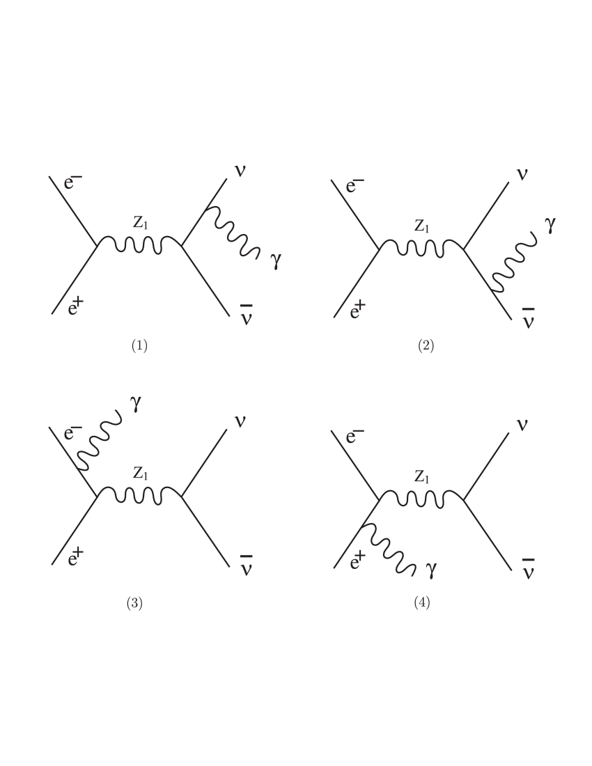
Figure 1: The Feynman diagrams contributing to the process $e^{+}e^{-}\rightarrow\nu\bar{\nu}\gamma$ in a 331 model (1, 2) when the $Z_{1}$ vector boson is produced on mass-shell and the SM (3, 4) diagrams for initial-state radiation.

However, in order to improve the limits on the magnetic moment and the electric dipole moment of the tau-neutrino, in our calculation to the process $e^{+}e^{-}\to\nu\bar{\nu}\gamma$ we consider initial-state radiation, in this way the bounds on the dipole moments are stronger than those evaluated in previous studies by other authors. We neglect $W$ and photon exchange diagrams, which amount to $1\hskip 1.42262pt\%$ corrections in the relevant kinematic regime. The Feynman diagrams which give the most important contribution to the cross section are shown in Fig. 1.

Our aim in the present paper is to analyze the reaction $e^{+}e^{-}\rightarrow\nu\bar{\nu}\gamma$ in the framework of a 331 model and we attribute an anomalous magnetic moment (MM) and an electric dipole moment (EDM) to a massive tau-neutrino. This process serve to set limits on the tau-neutrino MM and EDM. In this paper, we take advantage of this fact to set limits on $\mu_{\nu_{\tau}}$ and $d_{\nu_{\tau}}$ for various values of the mixing angle $\phi$ of the 331 model, according to Refs. Cogollo ; Hoang .

The L3 Collaboration L3 evaluated the selection efficiency using detector-simulated $e^{+}e^{-}\rightarrow\nu\bar{\nu}\gamma(\gamma)$ events, random trigger events, and large-angle $e^{+}e^{-}\rightarrow e^{+}e^{-}$ events. From Fig. 1 of Ref. L3 the process $e^{+}e^{-}\to\nu\bar{\nu}\gamma$ with $\gamma$ emitted in the initial state is the lone background in the $[44.5^{0},135.5^{0}]$ angular range (white histogram). From the same figure in this angular interval that is $-0.7<\cos\theta_{\gamma}<0.7$ we see that only 6 events were found, this is the real background, not 14 events. In this case a simple method Data2010 ; Rick ; Bayatian is that at 1$\sigma$ level ($68\hskip 1.42262pt\%\hskip 5.69054ptC.L$) for a null signal the number of observed events should not exceed the fluctuation of the estimated background events: $N=N_{B}+\sqrt{N_{B}}$. Of course, this method is good only when $N_{B}$ is sufficiently large (i.e. when the Poisson distribution can be approximated with a gaussian Data2010 ; Rick ; Bayatian ) but for $N_{B}>10$ it is a good approximation. This means that at $1\sigma$ level ($68\hskip 1.42262pt\%\hskip 5.69054ptC.L.$) the limits on the non-standard parameters are found replacing the equation for the total number of events expected $N=6+\sqrt{6}$ in the expression $N=\sigma(\phi,\mu_{\nu_{\tau}},d_{\nu_{\tau}}){\cal L}$. The distributions of the photon energy and the cosine of its polar angle are consistent with SM predictions.

This paper is organized as follows: In Sec. II we present the calculation of the process $e^{+}e^{-}\rightarrow\nu\bar{\nu}\gamma$ in the context of a 331 model. Finally, we present our results and conclusions in Sect. III.

II The Total Cross Section

In this section we calculate the total cross section for the reaction $e^{+}e^{-}\rightarrow\nu\bar{\nu}\gamma$ using the neutral current lagrangian given in Eqs. (9) and (10) of Ref. Cogollo for the 331 model for diagrams 1-4 of Fig. 1. A characteristic interesting from this model is that is independent of the mass of the additional $Z_{2}$ heavy gauge boson and so we have the mixing angle $\phi$ between the $Z_{1}$ and $Z_{2}$ bosons as the only additional parameter. The respective transition amplitudes are thus given by

$${\cal M}_{1} =\frac{-g^{2}}{4\cos^{2}\theta_{W}(l^{2}-m^{2}_{\nu})}\Bigl{[}\bar{u}(p_{3})\Gamma^{\alpha}(\l\hbox to0.0pt{\hss/}+m_{\nu})\gamma^{\beta}\Bigl{(}\cos\phi+\frac{1-2\sin^{2}\theta_{W}}{\sqrt{3-4\sin^{2}\theta_{W}}}\sin\phi\Bigr{)}v(p_{4})\Bigr{]}$$

$$\frac{(g_{\alpha\beta}-p_{\alpha}p_{\beta}/M^{2}_{Z_{1}})}{\Bigl{[}(p_{1}+p_{2})^{2}-M^{2}_{Z_{1}}-i\Gamma^{2}_{Z_{1}}\Bigr{]}}\Bigl{[}\bar{u}(p_{2})\gamma^{\alpha}\Bigl{(}\cos\phi-\frac{\sin\phi}{\sqrt{3-4\sin^{2}\theta_{W}}}\Bigr{)}(g_{\mbox{v}}-g_{A}\gamma_{5})v(p_{1})\Bigr{]}\epsilon^{\lambda}_{\alpha},$$

$${\cal M}_{2} =\frac{-g^{2}}{4\cos^{2}\theta_{W}(l^{{}^{\prime}2}-m^{2}_{\nu})}\Bigl{[}\bar{u}(p_{3})\gamma^{\beta}\Bigl{(}\cos\phi+\frac{1-2\sin^{2}\theta_{W}}{\sqrt{3-4\sin^{2}\theta_{W}}}\sin\phi\Bigr{)}(l\hbox to0.0pt{\hss/}^{\prime}+m_{\nu})\Gamma^{\alpha}v(p_{4})\Bigr{]}$$

$$\frac{(g_{\alpha\beta}-p_{\alpha}p_{\beta}/M^{2}_{Z_{1}})}{\Bigl{[}(p_{1}+p_{2})^{2}-M^{2}_{Z_{1}}-i\Gamma^{2}_{Z_{1}}\Bigr{]}}\Bigl{[}\bar{u}(p_{2})\gamma^{\alpha}\Bigl{(}\cos\phi-\frac{\sin\phi}{\sqrt{3-4\sin^{2}\theta_{W}}}\Bigr{)}(g_{\mbox{v}}-g_{A}\gamma_{5})v(p_{1})\Bigr{]}\epsilon^{\lambda}_{\alpha},$$

$${\cal M}_{3} =\frac{-g^{2}}{4\cos^{2}\theta_{W}(k^{2}-m^{2}_{e})}\Bigl{[}\bar{u}(p_{3})\gamma^{\alpha}\Bigl{(}\cos\phi+\frac{1-2\sin^{2}\theta_{W}}{\sqrt{3-4\sin^{2}\theta_{W}}}\sin\phi\Bigr{)}v(p_{4})\Bigr{]}$$

$$\frac{(g_{\alpha\beta}-p_{\alpha}p_{\beta}/M^{2}_{Z_{1}})}{\Bigl{[}(p_{1}+p_{2})^{2}-M^{2}_{Z_{1}}-i\Gamma^{2}_{Z_{1}}\Bigr{]}}\Bigl{[}\bar{u}(p_{2})\gamma^{\alpha}(k\hbox to0.0pt{\hss/}+m_{e})\gamma^{\beta}\Bigl{(}\cos\phi-\frac{\sin\phi}{\sqrt{3-4\sin^{2}\theta_{W}}}\Bigr{)}(g_{\mbox{v}}-g_{A}\gamma_{5})v(p_{1})\Bigr{]}\epsilon^{\lambda}_{\alpha},$$

and

$${\cal M}_{4} =\frac{-g^{2}}{4\cos^{2}\theta_{W}(k^{{}^{\prime}2}-m^{2}_{e})}\Bigl{[}\bar{u}(p_{3})\gamma^{\alpha}\Bigl{(}\cos\phi+\frac{1-2\sin^{2}\theta_{W}}{\sqrt{3-4\sin^{2}\theta_{W}}}\sin\phi\Bigr{)}v(p_{4})\Bigr{]}$$

$$\frac{(g_{\alpha\beta}-p_{\alpha}p_{\beta}/M^{2}_{Z_{1}})}{\Bigl{[}(p_{1}+p_{2})^{2}-M^{2}_{Z_{1}}-i\Gamma^{2}_{Z_{1}}\Bigr{]}}\Bigl{[}\bar{u}(p_{2})\gamma^{\beta}\Bigl{(}\cos\phi-\frac{\sin\phi}{\sqrt{3-4\sin^{2}\theta_{W}}}\Bigr{)}(g_{\mbox{v}}-g_{A}\gamma_{5})(k\hbox to0.0pt{\hss/}^{\prime}+m_{e})\gamma^{\alpha}v(p_{1})\Bigr{]}\epsilon^{\lambda}_{\alpha},$$

where

$$\Gamma^{\alpha}=eF_{1}(q^{2})\gamma^{\alpha}+\frac{ie}{2m_{\nu}}F_{2}(q^{2})\sigma^{\alpha\mu}q_{\mu}+eF_{3}(q^{2})\gamma_{5}\sigma^{\alpha\mu}q_{\mu},$$ (5)

is the neutrino electromagnetic vertex, $e$ is the charge of the electron, $q^{\mu}$ is the photon momentum and $F_{1,2,3}(q^{2})$ are the electromagnetic form factors of the neutrino, corresponding to charge radius, MM and EDM, respectively, at $q^{2}=0$ Escribano ; Vogel , while $\epsilon^{\lambda}_{\alpha}$ is the polarization vector of the photon. $l$ and $k$ stands for the momentum of the virtual neutrino and antineutrino respectively.

The MM, EDM and the mixing angle $\phi$ of the 331 model give a contribution to the total cross section for the process $e^{+}e^{-}\rightarrow\nu\bar{\nu}\gamma$ of the form:

$$\sigma(e^{+}e^{-}\rightarrow\nu\bar{\nu}\gamma) = \int\biggl{\{}\frac{\alpha^{2}}{96\pi}\left(\kappa^{2}\mu^{2}_{B}+d^{2}_{\nu_{\tau}}\right)\left[\frac{s-2\sqrt{s}E_{\gamma}+\frac{1}{2}E^{2}_{\gamma}\sin^{2}\theta_{\gamma}}{(s-M^{2}_{Z_{1}})^{2}+M^{2}_{Z_{1}}\Gamma^{2}_{Z_{1}}}\right]\Bigr{.}$$

$$+ \Bigl{.}\frac{\alpha^{2}}{64\pi}\Bigl{(}\kappa\mu_{B}+d_{\nu_{\tau}}\Bigr{)}\Biggl{(}\frac{s/E^{2}_{\gamma}-2\sqrt{s}/E_{\gamma}}{1-\cos^{2}\theta_{\gamma}}\Biggr{)}\Bigr{.}$$

$$\times \Bigl{.}\left[\frac{\Bigl{(}1-s(1-2E_{\gamma}/\sqrt{s})/M^{2}_{Z}\Bigr{)}\left((1-E_{\gamma}/\sqrt{s})^{2}+E^{2}_{\gamma}\cos^{2}\theta_{\gamma}/s\right)}{\left(s(1-2E_{\gamma}/\sqrt{s})-M^{2}_{Z_{1}}\right)^{2}+M^{2}_{Z_{1}}\Gamma^{2}_{Z_{1}}}\right]\Bigr{.}$$

$$+ \Bigl{.}\frac{\alpha^{2}}{32\pi}\Biggl{(}\frac{s/E^{2}_{\gamma}-2\sqrt{s}/E_{\gamma}}{1-\cos^{2}\theta_{\gamma}}\Biggr{)}\left[\frac{(1-E_{\gamma}/\sqrt{s})^{2}+E^{2}_{\gamma}\cos^{2}\theta_{\gamma}/s}{\Bigl{(}s(1-2E_{\gamma}/\sqrt{s})-M^{2}_{Z_{1}}\Bigr{)}^{2}+M^{2}_{Z_{1}}\Gamma^{2}_{Z_{1}}}\right]\biggr{\}}$$

$$\times \left[\frac{1-4x_{W}+8x^{2}_{W}}{x^{2}_{W}(1-x_{W})^{2}}\right]\left(\cos\phi-\frac{\sin\phi}{\sqrt{3-4x_{W}}}\right)^{2}\left(\cos\phi+\frac{(1-2x_{W})}{\sqrt{3-4x_{W}}}\sin\phi\right)^{2}$$

$$\times {E_{\gamma}dE_{\gamma}d\cos\theta_{\gamma}},$$

where $x_{W}\equiv\sin^{2}\theta_{W}$ and $E_{\gamma}$, $\cos\theta_{\gamma}$ are the energy and the opening angle of the emitted photon.

It is useful to consider the smallness of the mixing angle $\phi$, as indicated in the Eq. (14), to approximate the cross section in Eq. (6) by its expansion in $\phi$ up to the linear term: $\sigma=(\kappa^{2}\mu^{2}_{B}+d^{2}_{\nu_{\tau}})[A+B(\phi)]+(\kappa\mu_{B}+d_{\nu_{\tau}})[C+D(\phi)]+E+F(\phi)+O(\phi^{2})$, where $A$, $B$, $C$, $D$, $E$ and $F$ are constants which can be evaluated. Such an approximation for deriving the limits of $\mu_{\nu_{\tau}}$ and $d_{\nu_{\tau}}$ is more illustrative and easier to manipulate.

For $\phi<1$, the total cross section for the process $e^{+}e^{-}\rightarrow\nu\bar{\nu}\gamma$ is given by

$$\sigma(e^{+}e^{-}\rightarrow\nu\bar{\nu}\gamma)=(\mu^{2}_{\nu_{\tau}}+d^{2}_{\nu_{\tau}})[A+B\phi]+(\kappa\mu_{B}+d_{\nu_{\tau}})[C+D\phi]+E+F\phi+O(\phi^{2}),$$ (7)

where $A$ explicitly is

$$A=\int\frac{\alpha^{2}}{96\pi}\left[\frac{1-4x_{W}+8x^{2}_{W}}{x^{2}_{W}(1-x_{W})^{2}}\right]\left[\frac{s-2\sqrt{s}E_{\gamma}+\frac{1}{2}E^{2}_{\gamma}\sin^{2}\theta_{\gamma}}{(s-M^{2}_{Z_{1}})^{2}+M^{2}_{Z_{1}}\Gamma^{2}_{Z_{1}}}\right]{E_{\gamma}dE_{\gamma}d\cos\theta_{\gamma}},$$ (8)

while $B$, $C$, $D$, $E$ and $F$ are given by

$$B=\int\frac{\alpha^{2}}{16\pi}\left[\frac{1-4x_{W}+8x^{2}_{W}}{x_{W}(1-x_{W})^{2}}\right]\left[\frac{1}{\sqrt{3-4x_{W}}}\right]\left[\frac{s-2\sqrt{s}E_{\gamma}+\frac{1}{2}E^{2}_{\gamma}\sin^{2}\theta_{\gamma}}{(s-M^{2}_{Z_{1}})^{2}+M^{2}_{Z_{1}}\Gamma^{2}_{Z_{1}}}\right]{E_{\gamma}dE_{\gamma}d\cos\theta_{\gamma}},$$ (9)

$$C= \int\frac{\alpha^{2}}{64\pi}\left[\frac{1-4x_{W}+8x^{2}_{W}}{x^{2}_{W}(1-x_{W})^{2}}\right]\left[\frac{s/E^{2}_{\gamma}-2\sqrt{s}/E_{\gamma}}{1-\cos^{2}\theta_{\gamma}}\right]$$ (10)

$$\times \left[\frac{\Bigl{(}1-s(1-2E_{\gamma}/\sqrt{s})/M^{2}_{Z}\Bigr{)}\left((1-E_{\gamma}/\sqrt{s})^{2}+E^{2}_{\gamma}\cos^{2}\theta_{\gamma}/s\right)}{\left(s(1-2E_{\gamma}/\sqrt{s})-M^{2}_{Z_{1}}\right)^{2}+M^{2}_{Z_{1}}\Gamma^{2}_{Z_{1}}}\right]{E_{\gamma}dE_{\gamma}d\cos\theta_{\gamma}},$$

$$D= \int\frac{\alpha^{2}}{16\pi}\left[\frac{1-4x_{W}+8x^{2}_{W}}{x_{W}(1-x_{W})^{2}}\right]\left[\frac{1}{\sqrt{3-4x_{W}}}\right]\left[\frac{s/E^{2}_{\gamma}-2\sqrt{s}/E_{\gamma}}{1-\cos^{2}\theta_{\gamma}}\right]$$ (11)

$$\times \left[\frac{\Bigl{(}1-s(1-2E_{\gamma}/\sqrt{s})/M^{2}_{Z}\Bigr{)}\left((1-E_{\gamma}/\sqrt{s})^{2}+E^{2}_{\gamma}\cos^{2}\theta_{\gamma}/s\right)}{\left(s(1-2E_{\gamma}/\sqrt{s})-M^{2}_{Z_{1}}\right)^{2}+M^{2}_{Z_{1}}\Gamma^{2}_{Z_{1}}}\right]{E_{\gamma}dE_{\gamma}d\cos\theta_{\gamma}},$$

$$E= \int\frac{\alpha^{2}}{32\pi}\left[\frac{1-4x_{W}+8x^{2}_{W}}{x_{W}^{2}(1-x_{W})^{2}}\right]$$ (12)

$$\times\left[\frac{s/E^{2}_{\gamma}-2\sqrt{s}/E_{\gamma}}{1-\cos^{2}\theta_{\gamma}}\right]\left[\frac{(1-E_{\gamma}/\sqrt{s})^{2}+E^{2}_{\gamma}\cos^{2}\theta_{\gamma}/s}{\Bigl{(}s(1-2E_{\gamma}/\sqrt{s})-M^{2}_{Z_{1}}\Bigr{)}^{2}+M^{2}_{Z_{1}}\Gamma^{2}_{Z_{1}}}\right]{E_{\gamma}dE_{\gamma}d\cos\theta_{\gamma}},$$

$$F= \int\frac{\alpha^{2}}{8\pi}\left[\frac{1-4x_{W}+8x^{2}_{W}}{x_{W}(1-x_{W})^{2}}\right]\left[\frac{1}{\sqrt{3-4x_{W}}}\right]$$ (13)

$$\times\left[\frac{s/E^{2}_{\gamma}-2\sqrt{s}/E_{\gamma}}{1-\cos^{2}\theta_{\gamma}}\right]\left[\frac{(1-E_{\gamma}/\sqrt{s})^{2}+E^{2}_{\gamma}\cos^{2}\theta_{\gamma}/s}{\Bigl{(}s(1-2E_{\gamma}/\sqrt{s})-M^{2}_{Z_{1}}\Bigr{)}^{2}+M^{2}_{Z_{1}}\Gamma^{2}_{Z_{1}}}\right]{E_{\gamma}dE_{\gamma}d\cos\theta_{\gamma}}.$$

The expression given for A corresponds to the cross section previously reported by T. M. Gould and I. Z. Rothstein T.M.Gould , while $B$, $C$, $D$, $E$ and $F$ comes from the contribution of the 331 model, of the interference and the SM contribution due to bremsstrahlung in which the photon is radiated to the initial electron or positron. Evaluating the limit when the mixing angle is $\phi=0$, the terms that depend of $\phi$ in (7) are zero and Eq. (7) is reduced to the expression (3) given in Ref. T.M.Gould , more the contribution of the interference and the contribution of the SM, respectively.

III Results and Conclusions

In order to evaluate the integral of the total cross section as a function of the parameters of the 331 model, that is to say, $\phi$, we require cuts on the photon angle and energy to avoid divergences when the integral is evaluated at the important intervals of each experiment. We integrate over $\theta_{\gamma}$ from $44.5^{o}$ to $135.5^{o}$ and $E_{\gamma}$ from 15 $GeV$ to 100 $GeV$ for various fixed values of the mixing angle $\phi=-3.979\times 10^{-3},0,1.309\times 10^{-4}$. Using the following numerical values: $\sin^{2}\theta_{W}=0.2314$, $M_{Z_{1}}=91.18$ $GeV$ and $\Gamma_{Z_{1}}=2.49$ $GeV$, we obtain the cross section $\sigma=\sigma(\phi,\mu_{\nu_{\tau}},d_{\nu_{\tau}})$.

For the mixing angle $\phi$ between $Z_{1}$ and $Z_{2}$ of the 331 model, we use the reported data of Cogollo et al. Cogollo :

$$-3.979\times 10^{-3}\leq\phi\leq 1.309\times 10^{-4},$$ (14)

with a $90\%$ C. L. Other limits on the mixing angle $\phi$ reported in the literature are given in Ref. Hoang .

As was discussed in Refs. T.M.Gould ; L3 ; Barnett ; Feldman , $N\approx\sigma(\phi,\mu_{\nu_{\tau}},d_{\nu_{\tau}}){\cal L}$, where $N=6+\sqrt{6}$ is the total number of $e^{+}e^{-}\rightarrow\nu\bar{\nu}\gamma$ events expected at $1\sigma$ level ($68\hskip 1.42262pt\%\hskip 5.69054ptC.L.$) as is mentioned in the introduction and ${\cal L}=137$ $pb^{-1}$, according to the data reported by the L3 Collaboration Ref. L3 and references therein. Taking this into consideration, we can get a limit for the tau-neutrino magnetic moment as a function of $\phi$ with $d_{\nu_{\tau}}=0$.

The values obtained for this limit for several values of the $\phi$ parameter are show in Table 1.

$\phi$	$\mu_{\nu_{\tau}}(10^{-6}\mu_{B})$	$d_{\nu_{\tau}}(10^{-17}e\mbox{cm})$
$-3.979\times 10^{-3}$	[-2.57, 2.42]	[-4,95, 4.66]
0	[-2.60, 2.48]	[-5.01, 4.78]
$1.309\times 10^{-4}$	[-2.62, 2.50]	[-5.05, 4.82]

Table 1. Limits on the $\mu_{\nu_{\tau}}$ magnetic moment and $d_{\nu_{\tau}}$ electric dipole moment at $68\%$ C. L. for different values of the mixing angle $\phi$ Cogollo . We have applied the cuts used by L3 for the photon angle and energy.

The results obtained in Table 1 are in agreement with the literature T.M.Gould ; H.Grotch ; L3 ; Escribano ; DELPHI ; J.M.Hernandez ; Perez ; F.Larios ; Gutierrez1 ; Gutierrez2 ; Gutierrez3 ; Gutierrez4 ; Gutierrez5 ; Aydin . However, if the mixing angle is $\phi=-2.1\times 10^{-3},0,1.32\times 10^{-4}$ Hoang , we obtained the results given in Table 2.

$\phi$	$\mu_{\nu_{\tau}}(10^{-6}\mu_{B})$	$d_{\nu_{\tau}}(10^{-17}e\mbox{cm})$
$-2.1\times 10^{-3}$	[-2.59, 2.44]	[-4.99, 4.70]
0	[-2.60, 2.48]	[-5.01, 4.78]
$1.32\times 10^{-4}$	[-2.64, 2.52]	[-5.09, 4.86]

Table 2. Limits on the $\mu_{\nu_{\tau}}$ magnetic moment and $d_{\nu_{\tau}}$ electric dipole moment at $68\%$ C. L. for different values of the mixing angle $\phi$ Hoang . We have applied the cuts used by L3 for the photon angle and energy.

The previous analysis and comments can readily be translated to the EDM of the $\tau$-neutrino with $\mu_{\nu_{\tau}}=0$. The resulting limits for the EDM as a function of $\phi$ are shown in Tables 1 and 2.

The incorporation of the diagrams with photon radiation in the initial state, as well as the statistical analysis gives a contribution of about $22\hskip 1.42262pt\%$ on the bounds of magnetic and electric dipole moments of the tau-neutrino, with respect to analysis in $Z_{1}$ boson resonance, that is to say $s=M^{2}_{Z_{1}}$.

We plot the total cross section in Fig. 2 as a function of the mixing angle $\phi$ for the limits of the magnetic moment given in Tables 1 and 2. Our results for the dependence of the differential cross section on the photon energy versus the cosine of the opening angle between the photon and the beam direction $(\theta_{\gamma})$ are presented in Fig. 3 for $\phi=-3.979\times 10^{-3}$ and $\mu_{\nu_{\tau}}=2.42\times 10^{-6}\mu_{B}$. In addition, the form of the distributions does not change significantly for the values $\phi$ and $\mu_{\nu_{\tau}}$ because $\phi$ and $\mu_{\nu_{\tau}}$ are very small in value, as shown in Tables 1-2. Finally, we plot the differential cross-section in Fig. 4 as a function of the photon energy for the limits of the magnetic moments given in Tables 1-2.

Other upper limits on the tau-neutrino magnetic moment reported in the literature are $\mu_{\nu_{\tau}}<3.3\times 10^{-6}\mu_{B}$ $(90\hskip 2.84526pt\%\hskip 2.84526ptC.L.)$ from a sample of $e^{+}e^{-}$ annihilation events collected with the L3 detector at the $Z_{1}$ resonance corresponding to an integrated luminosity of $137$ $pb^{-1}$ L3 ; $\mu_{\nu_{\tau}}\leq 2.7\times 10^{-6}\mu_{B}$ $(95\hskip 2.84526pt\%\hskip 2.84526ptC.L.)$ at $q^{2}=M^{2}_{Z_{1}}$ from measurements of the $Z_{1}$ invisible width at LEP Escribano ; $\mu_{\nu_{\tau}}\leq 2.62\times 10^{-6}$ in the effective Lagrangian approach at the $Z_{1}$ pole Maya ; $\mu_{\nu_{\tau}}<1.83\times 10^{-6}\mu_{B}$ $(90\hskip 2.84526pt\%\hskip 2.84526ptC.L.)$ from the analysis of $e^{+}e^{-}\rightarrow\nu\bar{\nu}\gamma$ at the $Z_{1}$-pole, in a class of $E_{6}$ inspired models with a light additional neutral vector boson Aytekin ; from the order of $\mu_{\nu_{\tau}}<O(1.1\times 10^{-6}\mu_{B})$ Keiichi Akama et al. derive and apply model-independent limits on the anomalous magnetic moments and the electric dipole moments of leptons and quarks due to new physics Keiichi . However, the limits obtained in Ref. Keiichi are for the tau-neutrino with an upper bound of $m_{\tau}<18.2$ $MeV$ which is the current experimental limit. It was pointed out in Ref. Keiichi however, that the upper limit on the mass of the electron neutrino and data from various neutrino oscillation experiments together imply that none of the active neutrino mass eigenstates is heavier than approximately 3 $eV$. In this case, the limits given in Ref. Keiichi are improved by seven orders of magnitude. The limit $\mu_{\nu_{\tau}}<5.4\times 10^{-7}\mu_{B}$ $(90\hskip 2.84526pt\%\hskip 2.84526ptC.L.)$ is obtained at $q^{2}=0$ from a beam-dump experiment with assumptions on the $D_{s}$ production cross section and its branching ratio into $\tau\nu_{\tau}$ A.M.Cooper , thus severely restricting the cosmological annihilation scenario G.F.Giudice . Our results in Tables 1 and 2 for $\phi=-3.979\times 10^{-3},0,1.309\times 10^{-4}$ and $\phi=-2.1\times 10^{-3},0,1.32\times 10^{-4}$ compare favorably with the limits obtained by the L3 Collaboration L3 , and with others limits reported in the literature T.M.Gould ; H.Grotch ; Escribano ; Maya .

In the case of the electric dipole moment, other upper limits reported in the literature are: $\mid d(\nu_{\tau})\mid\leq 5.2\times 10^{-17}\mbox{$e$ cm},\hskip 2.84526pt{\mbox{95\% C.L.}}$ Escribano and $\mid d(\nu_{\tau})\mid<O(2\times 10^{-17}\mbox{$e$ cm})$ Keiichi .

In summary, we conclude that the estimated limits for the tau- neutrino magnetic and electric dipole moments in the context of a 331 model compare favorably with the limits obtained by the L3 Collaboration, and complement previous studies on the dipole moments. In the limit $\phi=0$ our limits takes the value previously reported in Ref. T.M.Gould for the SM. On the other hand, it seems that in order to improve these limits it might be necessary to study direct CP-violating effects M.A.Perez . In addition, the analytical and numerical results for the total cross section have never been reported in the literature before and could be of some practical use for the scientific community.

Acknowledgments

We acknowledge support from CONACyT, SNI and PROMEP (México).

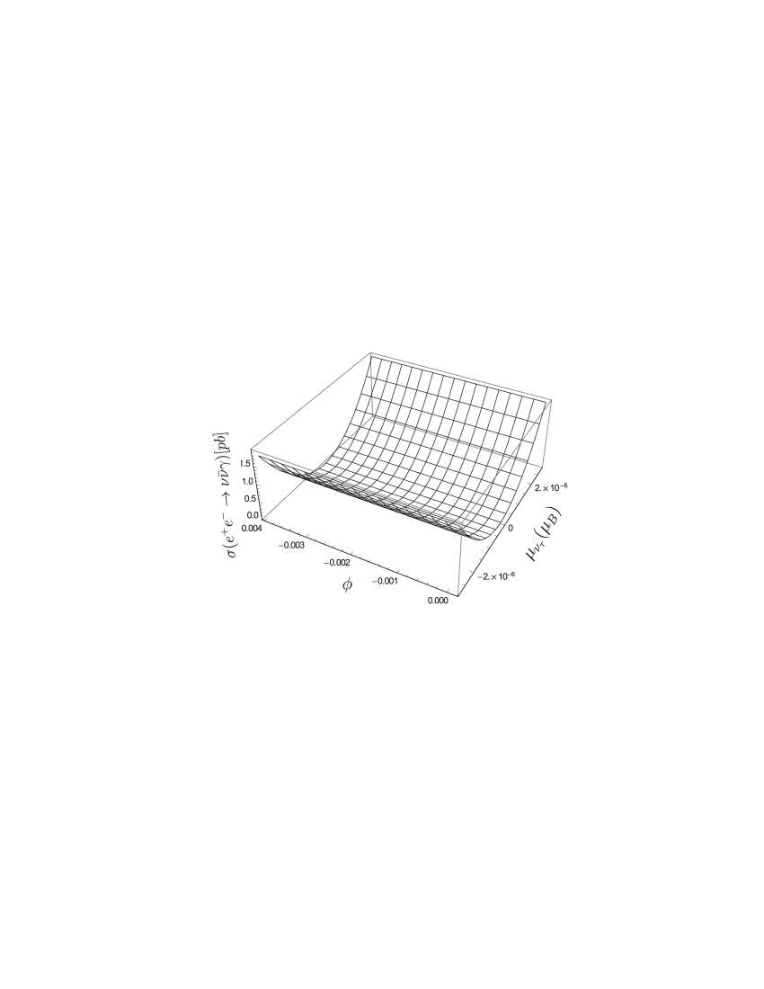
Figure 2: The total cross section for $e^{+}e^{-}\rightarrow\nu\bar{\nu}\gamma$ as a function of $\phi$ and $\mu_{\nu_{\tau}}$ (Tables 1, 2).

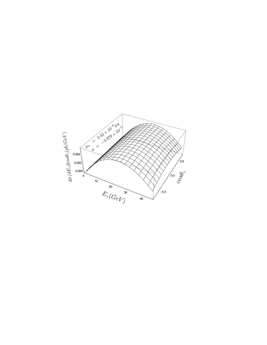
Figure 3: The differential cross section for $e^{+}e^{-}\rightarrow\nu\bar{\nu}\gamma$ as a function of $E_{\gamma}$ and $\cos\theta_{\gamma}$ for $\phi=-3.979\times 10^{-3}$ and $\mu_{\nu_{\tau}}=2.42\times 10^{-6}\mu_{B}$.

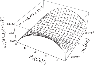
Figure 4: The differential cross section for $e^{+}e^{-}\rightarrow\nu\bar{\nu}\gamma$ as a function of $E_{\gamma}$ and $\mu_{\nu_{\tau}}$ with $\phi=-3.979\times 10^{-3}$.

References

• (1) S. L. Glashow, Nucl. Phys. 22, 579 (1961).
• (2) S. Weinberg, Phys. Rev. Lett. 19, 1264 (1967).
• (3) A. Salam, in Elementary Particle Theory, Ed. N. Svartholm (Almquist and Wiskell, Stockholm, 1968) 367.
• (4) R. N. Mohapatra and P. B. Pal, in Massive Neutrinos in Physics and Astrophysics, (World Scientific, Singapore, 1991).
• (5) M. Fukugita and T. Yanagida, Physics of Neutrinos and Applications to Astrophysics, (Springer, Berlin, 2003).
• (6) A. Cisneros, Astrophys. Space Sci. 10, 87 (1971).
• (7) R.W. Robinett, Phys. Rev. D26, 2388 (1982).
• (8) M. Green and J. Schwarz, Phys. Lett. B149, 117 (1984).
• (9) G. Senjanovic, Nucl. Phys. B153, 334 (1979).
• (10) G. Senjanovic and R. N. Mohapatra, Phys. Rev. D12, 1502 (1975).
• (11) U. Baur et al., Phys. Rev. D35, 297 (1987).
• (12) F. Pisano and V. Pleitez, Phys. Rev. D46, 410 (1992).
• (13) J. C. Montero, F. Pisano and V. Pleitez, Phys. Rev. D47, 2918 (1993).
• (14) Hoang Ngoc Long et al., Phys. Rev. D53, 437 (1996).
• (15) T. M. Gould and I. Z. Rothstein, Phys. Lett. B333, 545 (1994).
• (16) H. Grotch and R. Robinet, Z. Phys. C39, 553 (1988).
• (17) D. Cogollo et al., Mod. Phys. Lett. A23, 3405 (2009).
• (18) L3 Collab. M. Acciarri et al., Phys. Lett. B412, 201 (1997).
• (19) K. Nakamura et al., (Particle Data Group), J. Phys. G37, 075021 (2010).
• (20) Rick S. Gupta and James D. Wells, arXiv: 1110.0824 [hep-ph].
• (21) G. L. Bayatian et al., (CMS Collaboration), J. Phys. G34, 995 (2007).
• (22) R. Escribano and E. MassΓ³, Phys. Lett. B395, 369 (1997).
• (23) P. Vogel and J. Engel, Phys. Rev. D39, 3378 (1989).
• (24) R. M. Barnett et al., Phys. Rev. D54, 166 (1996).
• (25) G. J. Feldman and R. D. Cousins, Phys. Rev. D57, 3873 (1998).
• (26) DELPHI Collaboration, Z. Phys. C74, 577 (1997).
• (27) J. M. HernΓ‘ndez et al., Phys. Rev. D60, 013004 (1999).
• (28) M. A. PΓ©rez, G. Tavares-Velasco and J. J. Toscano, Int. J. Mod. Phys. A19, 159 (2004).
• (29) F. Larios, M. A. PΓ©rez, G. Tavares-Velasco, Phys. Lett. B531, 231 (2002).
• (30) A. GutiΓ©rrez-RodrΓ­guez et al., Phys. Rev. D58, 117302 (1998).
• (31) A. GutiΓ©rrez-RodrΓ­guez et al., Rev. Mex. de FΓ­s. 45, 249 (1999).
• (32) A. GutiΓ©rrez-RodrΓ­guez et al., Acta Physica Slovaca 53, 293 (2003).
• (33) A. GutiΓ©rrez-RodrΓ­guez et al., Phys. Rev. D69, 073008 (2004).
• (34) A. GutiΓ©rrez-RodrΓ­guez et al., Phys. Rev. D74, 053002 (2006).
• (35) C. Aydin, M. Bayar and N. Kilic, arXiv: hep-ph/0603080.
• (36) M. Maya, M. A. PΓ©rez, G. Tavares-Velasco, B. Vega, Phys. Lett. B434, 354 (1998).
• (37) Aytekin Aydemir and Ramazan Sever, Mod. Phys. Lett. A16 7, 457 (2001).
• (38) Keiichi Akama, Takashi Hattori and Kazuo Katsuura, Phys. Rev. Lett. 88, 201601 (2002).
• (39) A. M. Cooper-Sarkar et al., Phys. Lett. B280, 153 (1992).
• (40) G. F. Giudice, Phys. Lett. B251, 460 (1990).
• (41) M. A. PΓ©rez and F. RamΓ­rez-Zavaleta, Phys. Lett. B609, 68 (2005).
Refer to caption