Mesoscopic approach to minority games in herd regime

Abstract

We study minority games in efficient regime. By incorporating the utility function and aggregating agents with similar strategies we develop an effective mesoscale notion of state of the game. Using this approach, the game can be represented as a Markov process with substantially reduced number of states with explicitly computable probabilities. For any payoff, the finiteness of the number of states is proved. Interesting features of an extensive random variable, called aggregated demand, viz. its strong inhomogeneity and presence of patterns in time, can be easily interpreted. Using Markov theory and quenched disorder approach, we can explain important macroscopic characteristics of the game: behavior of variance per capita and predictability of the aggregated demand. We prove that in case of linear payoff many attractors in the state space are possible.

url]http://agf.statsolutions.eu

1 Introduction

Evolution of complex systems capable to adapt to varying environments by using shared memory is often considered as one of the fundamental dynamical problems in sciences. But large numbers of parameters a priori needed to describe them render difficult their exact analytic treatments. More efficient approaches are based on computational methods and direct modelling of adaptive systems with populations of agents. In course of development of these models it has been soon realized that even simplified approach with no communication between individuals, where the only dependence between them is given by common memory resource, appears to be useful and interesting. Among variety of multi-agent models, the minority game (MG) provides with a particularly intuitive representation of self-adaption where individuals reason out inductively and their rationality is limited. The MG was originally designed in Ref. [1] to account for profitability of playing in opposite to the plurality of decision makers. The model has been subsequently formalized in Refs. [2, 3] and became a well-established area of the game-theoretical, dynamical and statistical research [4].

The MG is a typical bottom-up construct and therefore usual definitions of the game first specify rules of behaviour for individuals. Then, piecing together microscopic variables, one defines higher-order quantities characterizing grander systems. In some cases, however, other descriptions are also possible, e.g. functions of state like score functions can be attributed to groups of agents without specifying agents individually [5]. And again, despite an apparent simplicity of basic rules of taking decisions by agents, adaptive abilities and phenomenology of populations playing MGs appear to be surprisingly non-trivial [4, 6]. As shown in Refs. [2, 7], phenomenology of MG depends qualitatively on game parameters. For example, the macroscopic quantity called aggregate attendance, or aggregate demand, pooling together individual choices, identifies three regimes of the MG: the random, cooperation and herd. After the authors of Refs. [7, 8], the latter case is also called efficient, because the total number of strategies is small, compared to the number of agents, and players have access to all available information. In addition, in this exceptional case the relatively small number of parameters enables analytical solutions.

The very first attempt of solving MG analytically was based on the method of statistical mechanics called the replica analysis. In order to find a more detailed analogy between statistical physics and MG, the group of Challet and Zhang [9, 10] limits their analysis to only two strategies per agent where the manifestation of cooperative effects is the strongest. The agents’ choice is then treated analogously to the projection of the particle’s spin on a quantization axis in space. The aggregate demand is split into two terms: the deterministic, forced by the quenched disorder, and a stochastic one that is further neglected. The quenched disorder term is related to systems in statistical physics when some parameters defining system’s behavior are stationary random variables, chosen when the system is created. Even such a simplified approach led to quite accurate analytical solutions for variance per capita as a function of the control parameter in the random regime. Additionally, the authors of Ref. [11] showed that properties of the MG in the symmetric phase depend on the initial conditions, what was confirmed numerically in Ref. [12]. If the initial conditions (i.e. the strategies) are drawn randomly, the system exhibits the so called quenched or frozen disorder. This theory, however, provides little knowledge on underlying dynamics of the game, i.e. on the evolution of utilities of strategies, and on existence of time patterns. An also it does not explain differences of macroscopic observables for different payoffs.

Another analytical approach, based on generating functional, is offered by Heimel and Coolen in Ref. [13]. This is the second most used technique, applicable to the statistical physics and a problem of disordered systems with random interactions. This method is in principle exact in the limit $N\rightarrow\infty$, although generally more difficult to apply than the replica procedure. The authors redefine the game for two strategies in such a way that instead of two independent utility values they operate only on one variable $q$ combining these two for each agent. As a result, the generalized MG is driven by only three equations, where the vector $\mathbf{q}=(q_{1},\ldots,q_{N})$ represents the state, and $N$ is the number of players. Then, the game is described in terms of the microscopic probability densities $Pr(\mathbf{q})$, where the discrete-time dynamics is replaced by the continuous-time one. Since the state depends on $N$, the behavior in the limit $N\rightarrow\infty$ can be examined. Similarly to the replica analysis, the method does not provide any insight into the game dynamics.

Concurrently, the group of Johnson introduced the so called crowd-anti- crowd theory offering approximate expressions for aggregate demand [14, 15]. Agents act as a crowd if they use the same strategy. If there is a group of agents using simultaneously the strategy anticorrelated to the first one, they make the opposite decisions and are considered as an anticrowd. There exist many different pairs of crowds and anticrowds at the same time. If sizes of crowd and anticrowd are similar, as it is the case in the cooperation regime, then the choices of these two groups cancel mutually and the volatility is kept small. If the crowd dominates, the majority of agents behave in the same manner and the volatility becomes large. It has been demonstrated that, considering fluctuations of the aggregated demand, analytical results are consistent with the numerical ones. Following the crowd-anticrowd reasoning, Jefferies et al. in Ref. [5] cast the game into the functional map, which reproduces the game when iterated. Such approach has a serious advantage compared to heuristically introduced rules in Refs. [2, 16], since it does not need to keep track of the labels for individual agents. In the definition of the functional map, those agents who hold the same combination of strategies are grouped together. In MG, individuals with the same strategies respond in the same way to all values of the global information set $\mu=\{0,1,\ldots,P-1\}$ ($P$ standing for the number of possible realizations of the winning decision history $\mu$), provided that the game starts with the same initial utilities for all the strategies. The grouping is done using the $S$-dimensional tensor, where S is the number of strategies per agent. Assuming that the Reduced Strategy Space (RSS) [3] is used, rows and columns of the tensor are of length $2P$ and each entry is equal to the number of agents holding a different combination of strategies. The concept of the state that is based on (i) utilities of pairwise different strategies and, (ii) history of past winning decisions, is subsequently introduced. Collecting above elements, a set of time-dependent equations, which reproduce the essential dynamics of the minority game, is written down. The authors figured out that MG can be interpreted as a stochastically disturbed deterministic system. To simplify the analysis, the stochastic term is skipped and attention is paid only to the deterministic part of the game. Then, the game is called the Deterministic MG. In the first studies of dynamics it is observed that the microscopic dynamics is affected markedly by the choice of the payoff function. The bahavior of the game is dictated by realization of distribution of agents over strategies and not just by specific game parameters. Hence, without knowledge about the disorder, the game cannot be classified to as being in either the efficient or inefficient regime. In Ref. [17], the dynamical approach is extended to the analysis of stochastic terms. The achieved analytical results provide correct explanation of variance per capita in herd regime, provided linear payoff, but no description of dynamics or predictabilities is given.

There are some similarities between the crowd-anticrowd theory and our mesoscopic approach introduced in Ref. [18] and further developed in this article. We incorporated the same concept of state as in Ref. [19] for the step-like payoff. We found however that the linear payoff requires different definition [18]. In the mesoscopic approach we aggregated agents playing the same strategy into fractions, and treated the fraction as one player. Such approach allowed us to represent the game in the herd regime as a Markov process, regardless of the payoff. We found it crucial to incorporate the stochastic transitions in the model - otherwise it is impossible to describe analytically the real dynamics. The mesoscopic approach was developed in stages, starting with Ref. [18]. First, we examined the system where fractions are of equal sizes. The following statements were proved: (i) the utility is bounded and the number of states is finite, (ii) the transition probabilities are both stochastic and deterministic. Incorporating these results we worked out the methodology of how to find the Markov representation of the process. Our analyses based on dynamics of the utility were mostly limited to the step-like payoff function and were technically hard to generalize. In addition, some important macroscopic observables, like demand variance per capita and predictability, were not yet analyzed and the quenched disorder was neglected. Here, we extend the method providing the consistent theory comprising different payoffs and quenched disorder. We start in section  3 where macroscopic differences between games with different payoffs are presented. The theory of how to describe the game in terms of the Markov process is provided in section 4. In many cases the explanation of macroscopic observables required relaxation of the assumption about equality of fraction sizes and we proved that such relaxation affects transition probabilities. We found it interesting that increasing the number of players does not make alike systems with equal and unequal fractions, even if in the latter case distributions of sizes are symmetric. Our analysis of the attractor structure of the Markov chain explains this and other dynamical phenomena observed in the herd regime, viz. oscillations of the aggregate attendance, its periodicity and predictability, or its dependence on the payoff form. These results are presented in section 4. The numerical studies of the periodicity in time are also found in Refs. [8, 20]. More comprehensive review of the literature is presented in Ref. [21].

2 The Formal Definition of the Minority Game

At each time step $t$, the $n$-th agent out of $N$ $(n=1,\ldots,N)$ takes an action $a_{\alpha_{n}}(t)$ according to some strategy $\alpha_{n}(t)$. The action $a_{\alpha_{n}}(t)$ takes either of two values: $-1$ or $+1$. An aggregated demand is defined

$$A(t)=\sum_{n=1}^{N}a_{\alpha_{n}^{\prime}}(t),$$ (1)

where $\alpha_{n}^{\prime}$ refers to the action according to the best strategy, as defined in eq. (3) below. Such defined $A(t)$ is the difference between numbers of agents who choose the $+1$ and $-1$ actions. Agents do not know each other’s actions but $A(t)$ is known to all agents. The minority action $a^{\ast}(t)$ is determined from $A(t)$

$$a^{\ast}(t)=-\mbox{sgn}\,A(t).$$ (2)

Each agent’s memory is limited to $m$ most recent winning, i.e. minority, decisions. Each agent has the same number $S\geq 2$ of devices, called strategies, used to predict the next minority action $a^{\ast}(t+1)$. The $s$th strategy of the $n$-th agent, $\alpha_{n}^{s}$ $(s=1,\ldots,S)$, is a function mapping the sequence $\mu$ of the last $m$ winning decisions to this agent’s action $a_{\alpha_{n}^{s}}$. Since there is $P=2^{m}$ possible realizations of $\mu$, there is $2^{P}$ possible strategies. At the beginning of the game each agent randomly draws $S$ strategies, according to a given distribution function $\rho(n):n\rightarrow\Delta_{n}$, where $\Delta_{n}$ is a set consisting of $S$ strategies for the $n$-th agent.

Each strategy $\alpha_{n}^{s}$, belonging to any of sets $\Delta_{n}$, is given a real-valued function $U_{\alpha_{n}^{s}}$ which quantifies the utility of the strategy: the more preferable strategy, the higher utility it has. Strategies with higher utilities are more likely chosen by agents.

There are various choice policies. In the popular greedy policy each agent selects the strategy of the highest utility

$$\alpha_{n}^{\prime}(t)=\arg\max_{s:\,\alpha_{n}^{s}\in\Delta_{n}}U_{\alpha_{n}^{s}}(t).$$ (3)

If there are two or more strategies with the highest utility then one of them is chosen randomly. The highest-utility strategy (3) used by the agent is called the active strategy, in contrast to passive strategies, unused at given moment. However, at any time all agents evaluate all their strategies, the active and passive ones. Each strategy $\alpha_{n}^{s}$ is given the payoff depending on its action $a_{\alpha_{n}^{s}}$

$$\Psi_{\alpha_{n}^{s}}(t)=-a_{\alpha_{n}^{s}}(t)\,g[A(t)],$$ (4)

where $g$ is an odd payoff function, e.g. the steplike $g(x)=\mbox{sgn}(x)$ [2], proportional $g(x)=x$ or scaled proportional $g(x)=x/N$. The learning process corresponds to updating the utility for each strategy

$$U_{\alpha_{n}^{s}}(t+1)=U_{\alpha_{n}^{s}}(t)+\Psi_{\alpha_{n}^{s}}(t),$$ (5)

such that every agent knows how good its strategies are.

3 Macroscopic observables

Macroscopic variables are understood here as random variables resulting from integration of random variables defined for individuals, over subsets of degrees of freedom of all individuals in the system. An example of such variable is the aggregate demand $A$, defined in the previous section. In this section we introduce and discuss two other particulary interesting macroscopic observables, viz. variance per capita and predictability. The variance per capita reflects the coordination between agents and is one of the most intriguing variables due to its nonmonotonic variation as a function of the control parameter $N/P$. Generally, variance per capita remains insensitive to the form of payoff function. In contrast, the predictabilities that detect the existence of patterns are susceptible to the payoff. Here, we demonstrate these phenomena paying attention mostly to the numerical results. The detailed analytical background is given later in section 4. Finally, time dependencies of the aggregate demand and utilities are presented, providing an insight into the origin of time patterns.

3.0.1 Observables as functions of the control parameter

The variance per capita for given game is defined using sample taken in subsequent time steps during time $T$ and assuming ergodicity of the process [2, 7]:

$$\sigma(A)^{2}=\frac{1}{T}\sum_{t=0}^{T}A(t)^{2}.$$ (6)

The variance, considered as a function of the control parameter $N/2^{m}$, represents a widely discussed result for MGs [2, 7], relevant to economic applications. For our present study it is important to note that its shape seems to be insensitive to form of the payoff function, as it is presented for two different payoffs and $m=3$ and $m=7$ in Fig. 1.

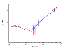
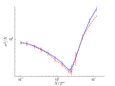
Figure 1: Variance per capita $\sigma(A)^{2}/N$ as a function of $N/P$ for S = 2, m = 3 (left) or $m=7$ (right). Two different payoff functions are used; full blue lines correspond to $g(x)=\mbox{sgn}\,(x)$ and dashed red lines to $g(x)=x$. Each point is a mean from ten games, error bars correspond to one standard deviation and curves are drawn to guide ones eye.

Similar premise for such payoff-independence is given by another macroscopic observable $H_{a}/N$, called predictability, where $H_{a}$ [22] is defined as

$$H_{a}=\frac{1}{P}\sum_{\mu=1}^{P}\langle a^{\ast}|\mu\rangle^{2},$$ (7)

where $\langle a^{\ast}|\mu\rangle$ is the conditional average of $a^{\ast}$ given $\mu$ and the mean is calculated over all $P$ histories.

The $H_{a}$ was demonstrated to be useful in detecting two interesting phases of the MG:

• The symmetric phase with $H_{a}\simeq 0$, where after the particular history $\mu(t)$ both signs of $a^{*}(t)$ appear with the same frequency. It is often claimed in literature [22, 16] that if $H_{a}=0$ then patterns in the time sequence do not exist. We find this condition to be the necessary but not sufficient one to state the lack of patterns. For example, if every appearance of given $\mu$ is followed by negative and positive minority decision alternately then $H_{a}=0$ and the predictable pattern exists. Indeed, such a behavior is observed for the MG in the herd regime and for $g(x)=x$ [18]. Hence, $H_{a}$ measures disproportions in frequencies between positive and negative minority decisions rather than detects patterns.

• The asymmetric phase with $H_{a}>0$ and existing predictable patterns. In the asymmetric phase, sign predictions significantly better than random are possible.

As presented in Figs 2, plots of $H_{a}/N$ seem to be independent of the payoff function, similarly to $\sigma^{2}/N$.

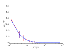
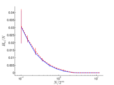
Figure 2: Predictability per capita $H_{a}/N$ as a function of $N/P$ for S = 2, m = 3 (left) or $m=7$ (right). Two different payoff functions are used: full blue lines correspond to $g(x)=\mbox{sgn}\,(x)$ and dashed red lines to $g(x)=x$. Each point is a mean from ten games, error bars correspond to one standard deviation and curves are drawn to guide ones eye.

By that means it was conjectured in early literature (cf. e.g. Ref. [23]) that only the payoff’s evenness is relevant to the macroscopic observables. Failure of this hypothesis is visible by analysing a modified macroscopic observable, we call demand predictability, which may be useful for prediction of the sign of demand. This variable is defined as

$$H_{A}=\frac{1}{P}\sum_{\mu=1}^{P}\langle A|\mu\rangle^{2}.$$ (8)

Plots of $H_{A}/N$ (cf. Fig. 3) exhibit its spectacular sensitivity to the payoff function in the effective regime, i.e. high $N/P$, in contrast to $H_{a}/N$ and $\sigma^{2}/N$.

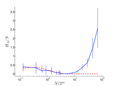
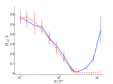
Figure 3: Demand predictability per capita $H_{A}/N$ as a function of $N/P$ for S = 2, m = 3 (left) or $m=7$ (right). Two different payoff functions are used: full blue lines correspond to $g(x)=\mbox{sgn}\,(x)$ and dashed red lines to $g(x)=x$. Each point is a mean from ten games, error bars correspond to one standard deviation and curves are drawn to guide ones eye.

For further analysis we decompose the conditional expected values into components corresponding to decisions $+1$ and $-1$:

$$\langle a^{\ast}|\mu\rangle = \langle a_{+}^{\ast}|\mu\rangle+\langle a_{-}^{\ast}|\mu\rangle,$$ (9)

where, formally

$$\langle a_{\pm}^{\ast}|\mu\rangle=\frac{1}{T}\sum_{t=1}^{T}a^{\ast}(t)\,\delta\big{(}\mu(t),\mu\big{)}\,\delta\big{(}a^{\ast}(t),\pm 1\big{)},$$ (10)

$\delta(i,j)$ standing for the Kronecker symbol. Similarly,

$$\langle A|\mu\rangle = \langle A_{+}|\mu\rangle+\langle A_{-}|\mu\rangle,$$ (11)

where

$$\langle A_{\pm}|\mu\rangle=\frac{1}{T}\sum_{t=1}^{T}A(t)\,\delta\big{(}\mu(t),\mu\big{)}\,\delta\big{(}\mbox{sgn}A(t),\pm 1\big{)}.$$ (12)

The case $H_{a}=0$ is possible if $\langle a^{\ast}|\mu\rangle=0$ for every $\mu$ which, as seen from Eq. (9), requires $|\langle a_{+}^{\ast}|\mu\rangle|=|\langle a_{-}^{\ast}|\mu\rangle|$. This means that the positive and negative values of $A(t)$ have to come with the same frequency. Similarly, the case $H_{A}=0$ happens if $|\langle A_{+}|\mu\rangle|=|\langle A_{-}|\mu\rangle|$ for every $\mu$, i.e. the positive and negative $A$ mutually compensate (cf. Eq. (11)). Combinations like (i) $H_{a}=0$ and $H_{A}>0$, and (ii) $H_{a}>0$ and $H_{A}=0$, are also possible.

3.1 Observables as functions of time

In order to examine MGs in the efficient regime, we performed a series of numerical simulations with different combinations of game parameters. We chose three representative cases: $(m,N)=(1,401),(2,1601),(5,1601)$, all with the number of strategies per agent $S=2$. All three games are in the efficient mode. In the first two cases the condition $NS\gg 2^{P}$ is fulfilled. In the third one it is not met and consequences of this fact will become clear later in the text. In all three experiments the full strategy space is used.

Figs 6, 6 and 6 present results for the steplike payoff function $g(x)=\mbox{sgn}(x)$: the time evolution of $A(t)$, the autocorrelation function $R(\tau)$ and the scatter plots of $A(t+2\cdot 2^{m})$ against $A(t)$, respectively. The same results for the proportional payoff function $g(x)=x$ are given in Figs 9, 9 and 9.

Even a fleeting glance at Figs 6 and 9 reveals regularities in $A(t)$ for both payoff functions but more regular and distinct for $g(x)=x$. In this case their period increases with the memory length $m$ and their maximal values are equal to the half of the population size $N/2$. This periodicity can be better seen using autocorrelation function $R(\tau)$ (cf. Figs 6 and 9) where $\tau$ is the correlation time. The autocorrelation $R$ exhibits statistically periodic peaks with

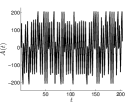
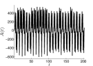
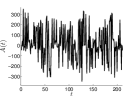
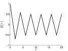
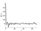
Figure 4: Time evolution of the aggregated demand $A(t)$ for three combinations of the population size $N$ and agent memory $m$: $N=401$, $m=1$ (left), $N=1601$, $m=2$ (middle) and $N=1601$, $m=5$ (right). Simulations were done for $S=2$ and $g(x)=\mbox{sgn}(x)$. Preferred values of $A$ are visible for all three games.

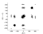
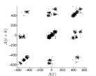
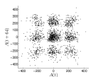
Figure 5: Autocorrelation function $R(\tau)$ for three combinations of the population size $N$ and agent memory $m$: $N=401$, $m=1$ (left), $N=1601$, $m=2$ (middle) and $N=1601$, $m=5$ (right). Simulations were done for $S=2$ and $g(x)=\mbox{sgn}(x)$. The highest values of $R$ are for $\tau=2\cdot 2^{m}$, except for $\tau=0$, for all games fulfilling the $NS\gg 2^{P}$ condition.

Figure 6: Plots of the aggregated demand $A(t+2\cdot 2^{m})$ vs. $A(t)$ for three combinations of the population size $N$ and agent memory $m$: $N=401$, $m=1$ (left), $N=1601$, $m=2$ (middle) and $N=1601$, $m=5$ (right). Simulations were done for $S=2$ and $g(x)=\mbox{sgn}(x)$. Apparent preferred levels of $A(t)$ are seen as clusters of points. For $m=1$ and $m=2$ points tend to flock around diagonals indicating positive correlation for $\tau=2\cdot 2^{m}$.

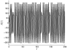
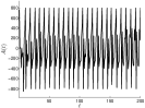
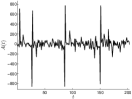
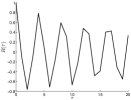
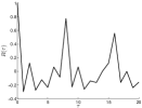
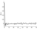
Figure 7: Time evolution of the aggregated demand $A(t)$ for three combinations of the population size $N$ and agent memory $m$: $N=401$, $m=1$ (left), $N=1601$, $m=2$ (middle) and $N=1601$, $m=5$ (right). Simulations were done for $S=2$ and $g(x)=x$. Preferred values of $A$ are visible for all three games.

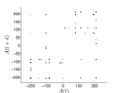
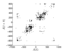
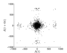
Figure 8: Autocorrelation function $R(\tau)$ for three combinations of the population size $N$ and agent memory $m$: $N=401$, $m=1$ (left), $N=1601$, $m=2$ (middle) and $N=1601$, $m=5$ (right). Simulations were done for $S=2$ and $g(x)=x$. The highest values of $R$ are for $\tau=2\cdot 2^{m}$, except for $\tau=0$, for all games fulfilling the $NS\gg 2^{P}$ condition.

Figure 9: Plots of the aggregated demand $A(t+2\cdot 2^{m})$ vs. $A(t)$ for three combinations of the population size $N$ and agent memory $m$: $N=401$, $m=1$ (left), $N=1601$, $m=2$ (middle) and $N=1601$, $m=5$ (right). Simulation was done for $S=2$ and $g(x)=x$. For $m=1$ and $m=2$ points tend to flock around diagonals, indicating positive correlation, but clusterization of points is not much pronounced.

periods $T=2\cdot 2^{m}$, as has been already observed in the efficient regime in Refs. [20, 5]. The autocorrelation is much less pronounced for games which do not meet the criterion $NS\gg 2^{P}$, as seen in Figs 6 and 9 (right). Relaxation of this criterion spoils periodicity of the aggregated demand. Similar observations can be done inspecting the $A(t+2\cdot 2^{m})$ vs. $A(t)$ scatter plots in Figs 6 and 9 where points for games fulfilling $NS\gg 2^{P}$ condition (left and middle panels in Figs 6 and 9) are stronger flocked around diagonals.

Another interesting feature of the aggregated demand, seen in the one-dimensional plots of $A(t)$, and better in the two-dimensional plots $A(t+2\cdot 2^{m})$ vs. $A(t)$, is an existence of preferred values of $A$. These preferred values show up as specles in the two-dimensional plots. The specles are better focused and more numerous for $g(x)=\mbox{sgn}(x)$ (Fig. 6) than for $g(x)=x$ (Fig. 9).

Time evolution of the utility functions appears to be a strongly mean-reverting process, independently of the payoff function, as seen e.g. in Figs 10. The more so, for the steplike payoff $g(x)=\mbox{sgn}(x)$ the utility is bounded to rather narrow belt $-2^{m}\leq U(t)\leq 2^{m}$, where here and in Fig. 10, $U(t)$ stands for the utility for any strategy. The formal proof of this statement is given in section 4. This feature is observed for any $N$ and $S$, provided the criterion $NS\gg 2^{P}$ is met.

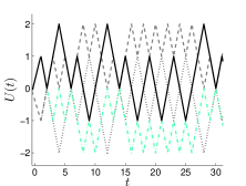
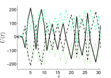
Figure 10: Trajectories of the utility function $U(t)$ for all strategies of the MG with $S=2$ and $m=1$ and $N$ high enough to ensure the $NS\gg 2^{P}$ regime. Two payoff functions are shown: the steplike $g(x)=\mbox{sgn}\,(x)$ (left) and the proportional $g(x)=x$ (right). Lines correspond to all different strategies. Note difference of vertical scales between panels.

4 The mesoscopic perspective

In this section we present the effective description of MG by redefining MG as a Markov chain. The general definition of state is found to be too complex for analytical treatments (cf. Sec. 4.1.1). Fortunately, in the herd regime, many agents have identical sets of strategies and their aggregation is possible. The set of individuals using the same strategies, called fraction, is further treated as a single agent (cf. Sec. 4.1.2). All possible fractions exist provided the game is large enough. Knowledge about utilities of pairwise different strategies and history of past winning decisions are enough to predict the action of any fraction. This set of parameters fully characterizes the system and is considered to specify its state. This definition is strictly suitable only for a step-like payoff function and can slightly vary for other payoffs (cf. Secs. 4.2 and 4.3).

Once the representation of the state is known, two methodologies are tried to explain the observations. In the simplified case we assumed the quenched disorder [17], i.e. an initial random choice of the strategy set at the start of the game and its later fixation, and in addition equality of fractions. However, not all observables are properly explained by that means and an extension of these assumptions is needed.

Transition probabilities can be calculated in two ways: before and after assignment of strategies to agents. We thus distinguish between a priori and a posteriori probability distribution of the aggregate demand.

Using this approach we manage to explain all observed phenomena. Finally, in Sec. 4.1.3 we define and study stability of this game in order to understand asymmetries observed in aggregate variables.

4.1 Definitions

4.1.1 The general concept of state

Since the MG represents a system with many degrees of freedom, dimensionality of states is expected to be large. In general, for each time step $t$, specification of state $x(t)$ consists of:

• The history of decisions $\mu(t)$,

• The set of strategies of all agents $\{\alpha_{n}^{s}\}_{n=1,\ldots,N}^{s=1,\ldots,S}$,

• The set of utilities for all strategies of all agents $\{U_{\alpha_{n}^{s}}(t)\}_{n=1,\ldots,N}^{s=1,\ldots,S}$,

• A function relating strategies to agents: $\rho(n):n\rightarrow\Delta_{n}$.

Although the history of decisions $\mu(t)$ partially stores information about the past of the process, transition probabilities depend only on the present state and the process is Markovian.

Substantial reduction of the number of state parameters and simplification of state description are possible if the game is large i.e. $NS\gg 2^{P}$ (cf. Secs. 4.2 and 4.3).

4.1.2 Fraction – definition and statistical properties

All agents behaving in the same manner - the fraction - can, in a sense, be treated as a whole. The fraction can be defined in two ways.

In the first approach it is a set of agents possessing a given, all the same, set of $S$ strategies. The set of pairwise different strategies is denoted as $\{\beta_{\kappa}\}_{\kappa=1}^{2^{P}}$. The number of agents in the fraction $\nu$, or the size of this fraction, is marked as $F_{\nu}$, where $\nu=\{1\ldots G\}$ and $G$ is the total number of different fractions. In large games, the system comprises agents of all possible fractions what results in constant $G$. In general, if strategies are assigned to agents randomly then $F_{\nu}$ are random variables. The strategy space consists of $2^{P}$ possible strategies and $G$ is represented by the number of $S$-combinations with repetition: $G=\binom{2^{P}+S-1}{S}$.

However, such definition of $G$ makes the expected values of the fraction sizes, ${\mathbb{E}}[F_{\nu}]$, not equal for different fractions, provided that strategies are randomly chosen from the uniform distribution. For example, assuming $S=2$, the fraction with two the same strategies, e.g. $\{\beta_{1},\beta_{1}\}$, is two times smaller than fraction with different strategies $\beta_{1}$ and $\beta_{2}$, where the ordering of strategies matters: $\{\beta_{1},\beta_{2}\}$ or $\{\beta_{2},\beta_{1}\}$. Therefore in the sequel we use another definition: the fraction is a set of agents using given sequence of strategies. The fraction size is now equal to $G=2^{PS}$. In such definition the strategy index $s\in\{1,\ldots,S\}$ is dummy. Nevertheless we use this approach because it radically simplifies the analysis without biasing the outcome, assuming assigning agents to fractions with equal probabilities. For example, consider the case $S=2$. Fractions’ indexes are assigned to each pair of strategies arbitrarily, e.g. as presented in Tab 1.

$F:$	$F_{1}$	$F_{2}$	$F_{3}$	$F_{4}$	$F_{5}$	$F_{6}$	$F_{7}$	$F_{8}$
$\beta:$	${\beta_{1},\beta_{1}}$	${\beta_{1},\beta_{2}}$	${\beta_{1},\beta_{3}}$	${\beta_{1},\beta_{4}}$	${\beta_{2},\beta_{1}}$	${\beta_{2},\beta_{2}}$	${\beta_{2},\beta_{3}}$	${\beta_{2},\beta_{4}}$

$F:$	$F_{9}$	$F_{10}$	$F_{11}$	$F_{12}$	$F_{13}$	$F_{14}$	$F_{15}$	$F_{16}$
$\beta:$	${\beta_{3},\beta_{1}}$	${\beta_{3},\beta_{2}}$	${\beta_{3},\beta_{3}}$	${\beta_{3},\beta_{4}}$	${\beta_{4},\beta_{1}}$	${\beta_{4},\beta_{2}}$	${\beta_{4},\beta_{3}}$	${\beta_{4},\beta_{4}}$

Table 1: One of possible assignments between fraction’s indexes and pairs of strategies

If at the beginning of the game strategies are drawn with equal probabilities, it corresponds to assigning agents to a specific fraction with probabilities $\frac{1}{G}$. Assume $W_{\nu}^{n}\in\{0,1\}$ is a random variable equal to 1 if agent $n$ belongs to fraction $\nu$. Then $F_{\nu}=\sum_{n=1}^{N}W_{\nu}^{n}$ follows the binomial distribution and $Pr(F_{\nu}=f_{\nu})=\binom{N}{f_{\nu}}(\frac{1}{G})^{f_{\nu}}(1-\frac{1}{G})^{N-f_{\nu}}$. Hence, ${\mathbb{E}}[F_{\nu}]=N/G$ or, if normalized, ${\mathbb{E}}[F_{\nu}/N]=1/G$.

For $N\rightarrow\infty$, we have ${\mathbb{V}ar}[F_{\nu}]\rightarrow\infty$ and ${\mathbb{V}ar}[F_{\nu}/N]\rightarrow 0$ . This means that, asymptotically for large $N$, (i) the absolute differences between sizes of fractions grow indefinitely, and (ii) percentages of population assigned to any fraction are equal. Hence, the larger the population, the larger expected difference between an actual size of a fraction $F_{\nu}$ and its expected value ${\mathbb{E}[F_{\nu}]}$.

4.1.3 Stability

The game is considered stable if for any strategy $\alpha_{n}$ the corresponding utility $U_{\alpha_{n}}(t)$ represents a mean-reverting stochastic process, i.e. the time-average of its increments vanishes after sufficiently long time. The MG has a build-in stabilization mechanism provided the game is large enough. The explanation is as follows.

Imagine that a subset $Z$ of strategies ($Z\subset\{\beta_{1},\ldots,\beta_{2^{P}}\}$) gets on average higher payoff than other subsets and the utilities in $Z$ grow up. Then, there always exists the same number of anticorrelated strategies with decreasing utility. The probability that an agent uses one of the strategies with a high utility is $1-(\#Z/2^{P})^{S}$, compared to those who use strategies with a low utility $(\#Z/2^{P})^{S}$ [18] ($\#Z$ is the number of elements in $Z$). Since the former probability is always higher, provided $S\geq 2$, then the most of population uses better strategies and their utility decreases, i.e. the game stabilizes. As long as fraction sizes are close to each other the above mechanism works and the game stays stable.

4.2 The payoff g(x) = sgn(x)

Here, the concept of the state for payoff $g(x)=sgn(x)$ is introduced. Applying it allows to represent the game as a Markov process and constitutes a consistent basis for analytical explanations of phenomena in the herd regime.

4.2.1 The concept of the state

Substantial reduction of the number of state parameters and simplification of state description are possible in our case. Agents can use identical strategies. The expected number of identical strategies in the whole population behaves asymptotically, for $N\rightarrow\infty$, like $NS/2^{P}$. The condition $NS\gg 2^{P}$ assures that the game stays in that asymptotic regime and the number of identical strategies is close to its asymptotic expected value. Identical strategies have the same utilities over the whole game, provided the initial values of utilities are the same, e.g. $U(0)=0$, for all strategies. It is thus enough to take into account only reduced set of pairwise different strategies $\{\beta_{\kappa}\}_{\kappa=1}^{2^{P}}$ and utilities defined on them, and therefore B and C from section 4.1.1 can be reduced:

• $\{\alpha_{n}^{s}\}_{n=1,\ldots,N}^{s=1,\ldots,S}\longrightarrow\{\beta_{\kappa}\}_{\kappa=1}^{2^{P}}$,

• $\{U_{\alpha_{n}^{s}}(t)\}_{n=1,\ldots,N}^{s=1,\ldots,S}\longrightarrow\{U_{\beta_{\kappa}}(t)\}_{\kappa=1}^{2^{P}}$.

Concerning point D, it is sufficient to find probabilities for agents to have strategies from the set of pairwise different strategies. The probability that given agent has any particular strategy from this set is equal to $1-(1-1/2^{P})^{S}$. For large $N$, the expected number of agents having this strategy is equal to $N(1-(1-1/2^{P})^{S})$. Therefore point D, i.e. a function ascribing strategies to agents, corresponding to the agent grouping tensor $\Omega$ of Ref. [5], can be dropped out entirely in this case. Note that this expected number in general differs from the actual number, which has some consequences explained later.

Finally, we describe states using $\mu(t)$ and the set of utilities for the complete set of $2^{P}$ pairwise different strategies $\{\beta_{\kappa}\}_{\kappa=1}^{2^{P}}$:

$$x(t)=[\,\mu(t),\,U_{1}(t),U_{2}(t),\ldots,U_{2^{P}}(t)\,].$$ (13)

Similar description of state was used in Ref. [5] but there are two important differences between these two: (i) the authors of Ref. [5] introduce a functional map giving time evolution of the system in any regime, and (ii) they degenerate the game by following mean values of demand, thus making the process deterministic and Markovian, and retaining possibility to randomize it perturbatively. Contrary to them, we do not degenerate the game. We consider it as a stochastic Markov process and eventually calculate the probability measure on states for the steplike payoff.

Utilities $\{U_{\beta_{\kappa}}(t)\}_{\kappa=1}^{2^{P}}$, considered as functions of time, are called trajectories. In the majority of cases and provided the number of observed time steps is large enough, strategies can be distinguished by their trajectories. The sufficient condition for all $2^{P}$ trajectories $U_{\beta_{\kappa}}(t)$ $(0\leq t\leq t_{0})$ to be distinguishable at $t_{0}$ is that all $2^{m}$ possible histories $\mu$ appear until then in a row. On the other hand, appearance of all histories $\mu$ until $t_{0}$, but not necessarily exclusively, represents a necessary condition of distinguishability for trajectories. Examples of MGs in the regime $NS\gg 2^{P}$ are shown in Figs 10 where trajectories are plotted for $m=1$ and $S=2$, and for two payoff functions further studied in this paper: $g(x)=\mbox{sgn}(x)$ and $g(x)=x$.

4.2.2 Finiteness of the number of states

In this section we demonstrate that for any $t$ the utility for any strategy is bounded from the bottom and top: $U_{min}\leq U(t)\leq U_{max}$, where $U_{min(max)}=-(+)\,2^{m}$. At least two approaches are possible. In the first approach one aggregates agents using strategies of a given utility value. Another one is based on fractions. Here we elaborate in detail on the former one and only present the sketch of proof of the latter.

Assume that at given time $t$ two different strategies have the same utilities. From Eq. (5) for the steplike payoff function it follows that after one time step these utilities can either differ by two units or remain the same. If the initial values of the utilities at $t=0$ are the same and after $\tau$ time steps at least one of them attains its extremal value, $U_{min}$ or $U_{max}$, then the trajectories cover the set of $2^{m}+1$ values (cf. Fig. 10, left)

$$U(\tau) \in \{u_{l}\}_{l=1}^{2^{m}+1}$$ (14)

$$= \{2^{m},2^{m}-2,\ldots,2,0,-2,\ldots,-2^{m}+2,-2^{m}\}.$$

Using this notation we have $u_{1}=U_{max}$ and $u_{2^{m}+1}=U_{min}$. The number of different strategies characterized by the same $u_{l}$ is given by combinatorics as the number of trajectories starting from 0 and ending at $u_{l}$ is

$$\#\{\beta_{\kappa}:U_{\beta_{\kappa}}=u_{l}\}=\left(\begin{array}[]{c}U_{max}\\ l-1\end{array}\right),\quad\quad l=1,\ldots,2^{m}+1.$$ (17)

The probability that the active strategy of the $n$-th agent $\alpha_{n}^{\prime}$ has utility $u_{l}$ is equal to

$$Pr\big{[}U_{\alpha_{n}^{\prime}}(t)=u_{l}\big{]}=\left\{\begin{array}[]{lr}1-Pr\big{[}U_{\alpha_{n}^{\prime}}(t)<u_{l}\big{]},&\quad l=1\\ Pr\big{[}U_{\alpha_{n}^{\prime}}(t)<u_{l-1}\big{]}-Pr\big{[}U_{\alpha_{n}^{\prime}}(t)<u_{l}\big{]},&\quad l>1\end{array}\right.$$ (20)

Using argumentation similar to that of Ref. [17], but extended to the full strategy space, one finds that

$$Pr\big{[}U_{\alpha_{n}^{\prime}}(t)<u_{l}\big{]} = \prod_{s=1}^{S}\Big{[}1-Pr\big{[}U_{\alpha_{n}^{s}}(t)\geq u_{l}\big{]}\Big{]}$$ (21)

$$= \Big{[}1-\frac{\#\{\beta_{\kappa}:U_{\beta_{\kappa}}\geq u_{l}\}}{2^{P}}\Big{]}^{S},$$

where, for $t=\tau$,

$$\#\{\beta_{\kappa}:U_{\beta_{\kappa}}\geq u_{l}\}=\sum_{j\geq l}\left(\begin{array}[]{c}U_{max}\\ j-1\end{array}\right).$$ (24)

Denoting $Pr_{max(min)}=Pr\big{[}U_{\alpha_{n}^{\prime}}(\tau)=U_{max(min)}\big{]}$, one sees from Eq. (20) that $Pr_{max}>Pr_{min}$. For any utility $u_{l}$, different than $U_{min}$ or $U_{max}$, the number of different strategies (17) is even. Even more, a half of strategies corresponding to each level $U_{min}<u_{l}<U_{max}$ suggests the opposite action than another half. According to Eq. (20), if two (or more) strategies have the same utility, then all have the same probability to be the best strategies for the $n$-th agent. This means that, if one excludes the best and the worst strategies, a half of remaining strategies recommends the same action as the best or the worst strategy. Hence the probability that an agent plays according to the strategy suggesting the same action as the best strategy is equal to

$$Pr\big{[}a_{\alpha_{n}^{\prime}}(\tau)=a_{\alpha^{B}}(\tau)\big{]} = Pr_{max}+\frac{1}{2}\big{(}1-Pr_{max}-Pr_{min}\big{)}$$ (25)

$$= \frac{1}{2}\big{(}1+Pr_{max}-Pr_{min}\big{)},$$

where $\alpha^{B}(t)$ is the best strategy from the whole set of strategies in the game, i.e. $U_{\alpha^{B}(t)}=u_{1}$, and $1-Pr_{max}-Pr_{min}$ refers to the probability that the agent’s best strategy is neither the worst nor the best of all strategies. The factor $\frac{1}{2}$ reflects that a half of strategies with non-extremal utilities suggests the same action as the best one. As $Pr_{max}>Pr_{min}$, from Eq. (25) it follows that if one of strategies has the utility $U_{max}$, then more than half of the population plays according to the best strategy. Subsequently, this subpopulation loose and gets the negative payoff. The rest are the winners and get the positive payoff. This mechanism bounds the utility to stay between $U_{min}$ and $U_{max}$. In addition, we know the formula for the fraction of agents playing the same action. For example, if $S=2$ and $m=1$ then $Pr_{max}=\frac{7}{16}$ and $Pr_{min}=\frac{1}{16}$. Hence, ${\mathbb{E}}[A]=\frac{3}{8}N$.

The analogical results are achieved when the concept of fraction is used. The number of different strategies characterized by the levels $u_{l}$ follows Eq. (17). Additionally, for all intermediate levels $U_{min}<u_{l}<U_{max}$ there exists the same number of strategies that suggest $+1$ and $-1$. Hence, all fractions that use one of these intermediate strategies compensate on average their mutual decisions. The last point is to find the number of fractions that use the best and the worst strategy, which are equal to $2^{PS}-(2^{P}-1)^{S}$ and $1$, respectively. For example, for $S=2$ and $m=1$ there are $G=2^{PS}=16$ fractions: seven using the best strategy and one using the worst one. Hence, ${\mathbb{E}}[A]=\frac{7}{16}N-\frac{1}{16}N=\frac{3}{8}N$, in compliance with the previous example.

4.2.3 The Markov process representation

The MG can be described in terms of the Markov process with the finite number of states. The $\mbox{sgn}\,A(x_{i})$ fully defines the utility and $\mu$ values of the next state and takes $\pm 1$. But in some specific states $A(x_{i})$ is always positive or negative and only one value of $\mbox{sgn}\,A(x_{i})$ appears. Hence, the transition may be either stochastic or deterministic and the transition probability is equal to

$$Pr(x_{j}|x_{i})=\frac{1}{2}\big{(}{\mathbb{E}}[\mbox{sgn}\,A(x_{i})]+1\big{)}.$$ (26)

The probability (26) depends only on the shape of the distribution of $A(x_{i})$. Using the concept of fractions, we redefine $A(x_{i})$ as follows:

$$A(x_{i})=\sum_{\nu}C_{\nu}(x_{i})F_{\nu},$$ (27)

where $C_{\nu}(x_{i})\in[-1,1]$ is a common action of all members of the fraction $\nu$ in the state $x_{i}$

$$C_{\nu}(x_{i})=\frac{1}{F_{\nu}}\sum_{n=1}^{F_{\nu}}a_{\alpha_{n}^{{}^{\prime}}(x_{i})}.$$ (28)

In other words, $C_{\nu}(x_{i})$ represents the aggregated demand per capita within fraction $\nu$. The $C_{\nu}(x_{i})$ depends on the action suggested in the state $x_{i}$ by the best strategy, or strategies, of the $\nu\,$-th fraction.

There are the following groups of fractions:

• Fractions with only one best strategy in the state $x_{i}$. All agents in the fraction react according to this strategy.

• Fractions with many best strategies where all best strategies in a given fraction suggest the same action in the state $x_{i}$. Although agents use different strategies, they all react identically.

• Fractions with many best strategies, where for each fraction some of the best strategies suggest the opposite action than another ones in the state $x_{i}$. Actions of agents are thus inhomogeneous and an overall action of such fraction is a random variable $C_{\nu}(x_{i})$, taking values $c_{\nu}^{\varphi}=\frac{-F_{\nu}+2\varphi}{F_{\nu}}$ for $\varphi=\{0,\ldots,F_{\nu}\}$, where $\varphi$ represents the possible numbers of agents acting $-1$ in the fraction $\nu$. This distribution depends on a proportion between best strategies suggesting opposite actions. Assuming there is $p^{+(-)}$ strategies suggesting the positive (negative) action, the $C_{\nu}(x_{i})$ obeys the binomial distribution

  $$Pr\big{(}C_{\nu}(x_{i})=c_{\nu}^{\varphi}\big{)}=\binom{F_{\nu}}{\varphi}\Big{(}\frac{p^{+}}{p^{+}+p^{-}}\Big{)}^{\varphi}\Big{(}\frac{p^{-}}{p^{+}+p^{-}}\Big{)}^{F_{\nu}-\varphi},$$ (29)

  where ${\mathbb{E}}[C_{\nu}(x_{i})]=-1+2\Big{(}\frac{p^{+}}{p^{+}+p^{-}}\Big{)}$ and ${\mathbb{V}ar}[C_{\nu}(x_{i})]=\frac{4}{F_{\nu}}\Big{(}\frac{p^{+}}{p^{+}+p^{-}}\Big{)}\Big{(}\frac{p^{-}}{p^{+}+p^{-}}\Big{)}$.

Fractions from the first two groups and suggesting $+1$ are marked with $d$, suggesting $-1$ are marked with $q$, and those belonging to the third group are indexed with $w$. Hence, Eq. (27) transforms into:

$$A(x_{i}) = \sum_{F_{d}:C_{d}(x_{i})=1}F_{d}-\sum_{F_{q}:C_{q}(x_{i})=-1}F_{q}$$ (30)

$$+\sum_{F_{w}:C_{w}(x_{i})\in[-1,+1]}C_{w}(x_{i})F_{w},$$

where

$${\mathbb{V}ar}[A(x_{i})]=4\sum_{F_{w}:C_{w}(x_{i})\in[-1,+1]}F_{w}\Big{(}\frac{p^{+}}{p^{+}+p^{-}}\Big{)}\Big{(}\frac{p^{-}}{p^{+}+p^{-}}\Big{)}.$$ (31)

Further analysis is relatively easy when fractions are of equal sizes and it complicates if their sizes are random.

The case of equal-size fractions

The system with the same numbers of agents per fraction we call the reference system and the corresponding MP – the reference MP. The $A(x_{i})$ is a random variable which can be expressed as:

$$A(x_{i})=\frac{N}{G}\bigl{(}D-Q+\sum_{F_{w}:C_{w}(x_{i})\in[-1,+1]}C_{w}(x_{i})\bigr{)},$$ (32)

where $D$ and $Q$ refer to the total numbers of fractions from the first two groups suggesting $+1$ and $-1$, respectively. If the state is deterministic then the components with opposite signs do not compensate and

$$|D-Q|>\mbox{max}\,\big{(}\sum_{F_{w}:C_{w}(x_{i})\in[-1,+1]}C_{w}(x_{i})\big{)}.$$ (33)

In the limit $NS\rightarrow\infty$, inequality (33) is satisfied always when the negative and positive components are unbalanced, i.e. $D\neq Q$. This can be proved at least in two ways.

The general proof uses the strong law of large numbers where the sample average $C_{w}(x_{i})$ converges almost surely to the expected value, i.e.

$$Pr(\lim_{N\rightarrow\infty}C_{w}(x_{i})={\mathbb{E}}\,\big{[}C_{w}(x_{i})\big{]})=1.$$ (34)

Each ${\mathbb{E}}\,\big{[}C_{w}(x_{i})\big{]}$ is equal to zero. Therefore the sum over $F_{w}:C_{w}(x_{i})\in[-1,+1]$ is equal to zero as well.

Another approach is applicable not only in the limit and requires separate analyses per state, as given in Example 2. For stochastic transitions there is always $D=Q$. For such states, $A(x_{i})$ has distribution symmetric around zero, ensuring that also distribution of $\mbox{sgn}\,A(x_{i})$ is symmetric and ${\mathbb{E}}[\mbox{sgn}\,A(x_{i})]=0$. Thus, transitions to two following states are equally probable.

Knowing how to distinguish the deterministic and stochastic states, the algorithm of defining the MP is the following:

1. Consider all $2^{m}$ initial states. Such states are characterized by $U_{\beta_{\kappa}}=0$ for all strategies $\kappa$ and different histories $\mu$. Due to equality of all strategies, two minority decisions are equally possible for each of initial states and the transition is stochastic. These minority decisions determine strategies that get positive or negative payoff. The updated $U$ and $\mu$ values determine $2^{m+1}$ next states.

2. If, in the next state, there are many best pairwise different strategies suggesting opposite actions, then $D=Q$ and, again, two minority decisions and two successive states are possible, and the transition is stochastic. Hence, two next states have to be determined.

3. If, in the next state, there are many best pairwise different strategies suggesting the same action, then $D\neq Q$ and the minority decision is determined by this action, and transition is deterministic.

4. If there is only one strategy characterized by the highest value of the utility, then $D\neq Q$ and the minority decision is determined by the best strategy, and transition is deterministic.

Here we illustrate how one can find subsequent states and their transition probabilities using the algorithm presented above (Example 1). Next, in the Example 2 we show how to check step-by-step that the transition is stochastic/deterministic assuming finite number of agents.

Example 1: transition scenarios for $m=1$ case

An example realization of the $A(t)$ for the reference MP is given in Fig. 11 (upper left). The estimated $A$-distribution is symmetric (upper right) and the distribution of $\mbox{sgn}(A)$ is symmetric likewise (lower right). The scatter plot of $A(t+\tau)$ as a function of $A(t)$, where $\tau=2^{m+1}$, indicates periodicity and existence of preferred values of $A$ (lower left).

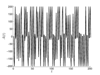
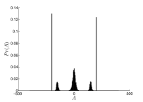
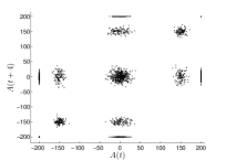
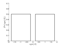
Figure 11: Time evolution of the aggregated demand $A(t)$ (upper left), Plots of the aggregated demand $A(t+2\cdot 2^{m})$ vs. $A(t)$ (lower left), Estimated $Pr(A)$ (upper right) and $Pr(\mbox{sgn}(A))$ (lower right) for the population size $N=400$ and agent memory $m=1$, $S=2$ strategies per agent and identical sizes of fractions.

In this case the complete specification of states and calculation of the transition matrix are relatively easy. All strategies are listed in Tab. 2.

$\mu$	$\beta_{1}$	$\beta_{2}$	$\beta_{3}$	$\beta_{4}$
-1	-1	-1	1	1
1	-1	1	-1	1

Table 2: Strategies for $m=1$

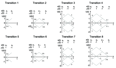
Figure 12: Trajectories of utilities for $m=1$.

Possible transition scenarios for the $m=1$ MG, represented as the Markov chain, are illustrated in Figs 12.

At the beginning of the game all utilities are equal to zero. Depending on the history $\mu$, only two initial states can exist: $x_{1}=[-1,0,0,0]$ and $x_{2}=[1,0,0,0]$. For each of these two states two further scenarios are equally possible, because the utilities of corresponding strategies are the same. The choice depends on the ratio between numbers of agents in two groups: one with $a=1$ and another one with $a=-1$. These scenarios are as follows.

• Being in the state $x_{1}$, the majority of agents use strategies suggesting $a=-1$. Then

  • the minority action in the next step is $a^{\ast}=1$,

  • strategies $\beta_{1}$ or $\beta_{2}$ give negative payoff,

  • strategies $\beta_{3}$ and $\beta_{4}$ give positive payoff.

  The system goes to the state $x_{3}=[1,-1,-1,1,1]$ (cf. Fig. 12, Transition 1) where $U_{\beta_{3}}=U_{\beta_{4}}=1$ and these strategies suggest different actions on the last history $\mu=1$. Similarly, there are two strategies with the utilities $U_{\beta_{1}}=U_{\beta_{2}}=-1$ suggesting different actions on $\mu=1$. Hence, there are two equiprobable scenarios, further described as Transitions 3 and 4.

• Being in the state $x_{1}$, the majority of agents use strategies suggesting $a=1$. Then

  • the minority action in the next step is $a^{\ast}=-1$,

  • strategies $\beta_{3}$ or $\beta_{4}$ give negative payoff,

  • strategies $\beta_{1}$ and $\beta_{2}$ give positive payoff.

  The system goes to the state $x_{11}=[-1,1,1,-1,-1]$ (cf. Fig. 12, Transition 2) where $U_{\beta_{1}}=U_{\beta_{2}}=1$ and give the same actions on the last history $\mu=-1$. Most of agents use these strategies (e.g. $3/4$ of the population, provided $S=2$) and the sole possibility is that the system goes to the state $x_{2}$.

• Being in the state $x_{3}$, the majority of agents use strategies suggesting $a=1$ and the system passes to $x_{5}$. In this state $U_{\beta_{3}}=U_{max}$ and $U_{\beta_{2}}=U_{min}$ (cf. Fig. 12, Transition 3). According to the reasoning from section 5.1, if one utility attains its maximal or minimal value, most agents use strategies suggesting the same action as the best strategy. Consequently, there is only one scenario possible in $x_{5}$: the best strategy, and all strategies giving the same output as the best one, loose and the system goes to the state $x_{4}$.

• Another possibility in $x_{3}$ is that most of agents decide $a=-1$ and the system goes to $x_{7}$. In this state $U_{\beta_{4}}=U_{max}$ and $U_{\beta_{1}}=U_{min}$ (cf. Fig. 12, Transition 4). Subsequently, the best strategy, and all strategies giving the same output as the best one, loose and the system goes to the state $x_{9}$. In $x_{9}$ both best strategies suggest the same for the last history $\mu=-1$. The majority of the population uses one of these best strategies and the system moves to $x_{1}$.

• These transitions are analogical to Transitions 1–4, but the initial state is $x_{2}$.

	$\mu$	$U_{1}$	$U_{2}$	$U_{3}$	$U_{4}$	$Pr(x_{i})$	${\mathbb{E}}\,[A(x_{i})]$	${\mathbb{V}ar}\,[A(x_{i})]$
$x_{1}$	-1	0	0	0	0	$\frac{1}{8}$	0	$\frac{N}{2}$
$x_{2}$	1	0	0	0	0	$\frac{1}{8}$	0	$\frac{N}{2}$
$x_{3}$	1	-1	-1	1	1	$\frac{1}{8}$	0	$\frac{N}{4}$
$x_{4}$	-1	1	-1	1	-1	$\frac{1}{8}$	0	$\frac{N}{4}$
$x_{5}$	-1	0	-2	2	0	$\frac{1}{16}$	$\frac{3}{8}N$	$\frac{N}{8}$
$x_{6}$	1	0	-2	2	0	$\frac{1}{16}$	$-\frac{3}{8}N$	$\frac{N}{8}$
$x_{7}$	1	-2	0	0	2	$\frac{1}{16}$	$\frac{3}{8}N$	$\frac{N}{8}$
$x_{8}$	-1	2	0	0	-2	$\frac{1}{16}$	$-\frac{3}{8}N$	$\frac{N}{8}$
$x_{9}$	-1	-1	-1	1	1	$\frac{1}{16}$	$\frac{1}{2}N$	$0$
$x_{10}$	1	1	-1	1	-1	$\frac{1}{16}$	$\frac{1}{2}N$	$0$
$x_{11}$	-1	1	1	-1	-1	$\frac{1}{16}$	$-\frac{1}{2}N$	$0$
$x_{12}$	1	-1	1	-1	1	$\frac{1}{16}$	$-\frac{1}{2}N$	$0$

Table 3: States $x_{i}$ $(i=1,\ldots,12)$, their probabilities $Pr(x_{i})$ and demands for $m=1$. The ${\mathbb{E}}\,[A(x_{i})]$ stands for the expected value of $A$ for the state $x_{i}$.

The states are listed in Tab. 3. These states and transitions are sufficient to define a memoryless representation of the MG with a transition graph displayed in Fig. 13.

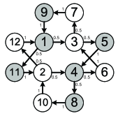
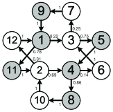
Figure 13: Diagrams of the Markov chain representation of the MG in the efficient regime for $m=1$. Numbers in circles represent the following states: $x_{1}=[-1,0,0,0,0]$, $x_{2}=[1,0,0,0,0]$, $x_{3}=[1,-1,-1,1,1]$, $x_{4}=[-1,1,-1,1,-1]$, $x_{5}=[-1,0,-2,2,0]$, $x_{6}=[1,0,-2,2,0]$, $x_{7}=[1,-2,0,0,2]$, $x_{8}=[-1,2,0,0,-2]$, $x_{9}=[-1,-1,-1,1,1]$, $x_{10}=[1,1,-1,1,-1]$, $x_{11}=[-1,1,1,-1,-1]$, $x_{12}=[1,-1,1,-1,1]$. States marked as grey incorporate $\mu=-1$ while the white ones $\mu=+1$. Values assigned to arrows reflect transition probabilities. Two cases are shown: equal fractions (left) and unequal ones where agents draw strategies with uniform probability (right). In the case of equal fractions, if transitions to two states are possible from a given state, both transition probabilities are the same.

Some of its states have the same expected demand ${\mathbb{E}}\,[A]$ over realizations of the game, e.g. ${\mathbb{E}}\,[A(x_{i})]=0$ ($i=1,...,4$), since the same numbers of agents play according to strategies recommending opposite actions. Using formulas (20-24) we can find ${\mathbb{E}}\,[A]$ for all states (cf. Tab. 3), consistently with observations in Fig. 11, where five clusters on the diagonal are found around values from Tab. 3. Our process is a stationary Markov chain for which the stationary Master Equation can be solved with respect to the state probabilities. Their values are given in Tab. 3, in the column marked $Pr(x_{i})$ $(i=1,\ldots,12)$. The state probabilities from Tab. 3 can be also used to find statistical periods of the demand

$$Pr\big{[}A(t)=A(t+\tau)\big{]} = \sum_{ij}\,\delta\big{[}A\big{(}x_{j}(t+\tau)\big{)},A\big{(}x_{i}(t)\big{)}\big{]}$$ (35)

$$\cdot Pr\big{[}x_{j}(t+\tau)\,|\,x_{i}(t)\big{]}\cdot Pr\big{[}x_{i}(t)\big{]},$$

where $\delta(x,y)$ stands for the Kronecker symbol. The maximal value of $7/16$ is found for $\tau=4$ and this explains why the largest correlation is found also for $\tau=4$ (cf. Figs 6 and 9).

Example 2: Deterministic transitions

Here, we show an example how to prove that the transition from a given state is deterministic provided that the system is a reference one and the game is in herd regime but not necessarily in the limit $NS\rightarrow\infty$. Additionally, we present that the transition can change if agents are assigned to fractions randomly.

Let us consider an arbitrarily chosen state for $S=2$ and $m=1$ where the transition is deterministic, e.g. $x_{5}$ defined as $x_{5}=[-1,0,-2,2,0]$. Assume that fractions’ indexes are assigned to each pair of strategies according to Tab. 1. Analyzing each fraction one finds that:

• For fractions $F_{11},F_{12},F_{15},F_{16}$ both strategies suggest $+1$. Hence $C_{\nu}(x_{i})=+1$, for $\nu\in\{11,12,15,16\}$.

• For fractions $F_{3},F_{7},F_{8},F_{9},F_{10},F_{14}$ strategy with higher $U$ suggests $+1$. As a result for these strategies $C_{\nu}(x_{i})=+1$, for $\nu\in\{3,7,8,9,10,14\}$.

• In fractions $F_{1},F_{2},F_{5},F_{6}$ both strategies suggest $-1$. Thus $C_{\nu}(x_{i})=-1$, for $\nu\in\{1,2,5,6\}$.

• Finally, fractions $F_{4},F_{13}$ have two strategies with equal probabilities but suggesting opposite actions. Hence, $C_{\nu}(x_{i})$, for $\nu\in\{4,13\}$, follows binomial distribution (29).

For the reference system (equal fractions) one can calculate ${\mathbb{E}}[A(x_{5})]=\frac{5}{16}N$. The uncertainty is introduced by agents belonging to fractions $F_{4},F_{13}$ because they choose $-1$ or $+1$ with the same probability. It means that $A(x_{5})\in\{\frac{3}{16}N\ldots\frac{5}{16}N\}$ and $\mathbb{V}ar[A(x_{5})]=N/8$. Hence, $A(x_{5})$ is always positive and $a^{*}(x_{5})=-1$, thus the successor state is determined unambiguously. Such analysis can be performed for arbitrary state which makes easy calculation of variance of the aggregate demand (cf. Tab. 3).

Any MG with $m>1$ in the efficient regime can be represented as a Markov process with a finite number of states. The same method as for $m=1$, but more demanding computationally, can be used to calculate state probabilities. The reasoning presented is strictly true only in the ideal case where subpopulations of agents in different fractions are equal, or if the system is considered a priori, i.e. before strategies are assigned to agents at the beginning of the game. In a posteriori analysis we consider the game where strategies are already assigned. In most cases such game is characterized by an inequality between sizes of fractions due to the initial randomness in the strategies’ generation process (quenched disorder). In Example 2, considering system a priori, the expected value ${\mathbb{E}}[A(x_{5})]$ remains the same but the variance changes distinctly enough to allow for appearance of negative samples. Considered a posteriori, also ${\mathbb{E}}[\widetilde{A}(x_{5})]$ is most likely biased compared to ${\mathbb{E}}[A(x_{5})]$. We show that some interesting phenomena, among them the sensitivity of the predictability $H_{A}$ to the payoff, appear only when the quenched disorder is taken into account i.e. imbalance between fractions exists.

The case of unequal-size fractions

If strategies are assigned randomly to agents then fraction sizes are likely to be unequal. Let us consider one of the simplest cases where strategies are drawn with equal probabilities, which corresponds to assigning an agent to any fraction with the probability $\frac{1}{G}$. Interestingly, numerical experiments show that in this case the reconstructed MP usually follows the sequence of states of the reference MP but the values of transition probabilities are not reproduced. This bias does not disappear even if the game is enlarged (see Figs 11 and 14).

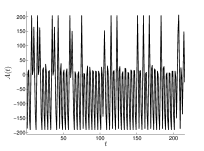
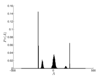
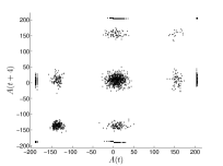
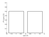
Figure 14: Time evolution of the aggregated demand ${A}(t)$ (upper left), Plots of the aggregated demand ${A}(t+2\cdot 2^{m})$ vs. ${A}(t)$ (lower left), Estimated $Pr({A})$ (upper right) and $Pr(\mbox{sgn}({A}))$ (lower right) for the population size $N=400$ and agent memory $m=1$, $S=2$ strategies per agent and unequal sizes of fractions.

The explanation is as follows.

States in the reference MP, where stochastic transition appears, are characterized by the same number of positive and negative components in formula (30). Calculating the transition probability we considered two cases: before and after assignment of strategies to agents, i.e. the a priori and a posteriori one.

Calculating a priori expected value of $\mbox{sgn}\,A$ we do not know yet the specific number of agents in the $\nu$-th fraction and we just operate on random variables:

$${\mathbb{E}}[\mbox{sgn}\,A(x_{i})] = {\mathbb{E}}\Big{[}\mbox{sgn}\sum_{\nu}C_{\nu}(x_{i})F_{\nu}\Big{]}$$ (36)

$$= {\mathbb{E}}\Big{[}\mbox{sgn}\big{(}\sum_{F_{d}:C_{d}(x_{i})=1}F_{d}-\sum_{F_{q}:C_{q}(x_{i})=-1}F_{q}$$

$$+\sum_{F_{w}:C_{w}(x_{i})\in[-1,+1]}C_{w}(x_{i})F_{w}\big{)}\Big{]}$$

Each fraction size $F_{\nu}$ obeys the same binomial distribution. Since we consider stochastic transitions in the reference system, then there is the same number of elements in the first and second sum of Eq. (36). The distribution of the third sum is symmetric around zero because it contains pairwise symmetric components. Thus, the distribution of $A(x_{i})$ is also symmetric, as well as the distribution of $\mbox{sgn}\,A(x_{i})$. By that means ${\mathbb{E}}[\mbox{sgn}\,A(x_{i})]=0$.

When strategies are assigned to agents, then the numbers of agents in fractions, $f_{\nu}$, are known and the system is considered as a posteriori. The ${\mathbb{E}}[\mbox{sgn}\,{A}(x_{i})]$ can be decomposed:

$${\mathbb{E}}[\mbox{sgn}\,{A}(x_{i})] = {\mathbb{E}}\Big{[}\mbox{sgn}\,\big{(}\sum_{f_{d}:C_{d}(x_{i})=1}f_{d}-\sum_{f_{q}:C_{q}(x_{i})=-1}f_{q}$$ (37)

$$+\sum_{f_{w}:C_{w}(x_{i})\in[-1,+1]}C_{w}(x_{i})f_{w}\big{)}\Big{]}.$$

Provided $S=2$, the last sum in Eq. (37) is symmetric around zero due to $C_{w}$ symmetry but the first two sums introduce a bias, shifting distribution of $A(x_{i})$. If $S>2$ then also the third term may be biased. Since ${\mathbb{V}ar}[F]\rightarrow\infty$ for $N\rightarrow\infty$, then considering only first two components one gets

$${\mathbb{V}ar}[\sum_{F_{d}:C_{d}(x_{i})=1}F_{d}-\sum_{F_{q}:C_{q}(x_{i})=-1}F_{q}]\rightarrow\infty,$$ (38)

which means that the probability of a large bias grows indefinitely with $N$.

If the a posteriori distribution of $A(x_{i})$ is shifted then the a posteriori distribution of $\mbox{sgn}\,A(x_{i})$ is asymmetric, regardless of a symmetry of the last term. Consequently, most likely ${\mathbb{E}}[\mbox{sgn}\,{A}(x_{i})]\neq 0$. The equality between ${\mathbb{E}}[\mbox{sgn}\,{A}(x_{i})]$ calculated using a priori distribution and ${\mathbb{E}}[\mbox{sgn}\,A(x_{i})]$ calculated using distribution a posteriori occurs only if numbers of agents per fraction are equal for all fractions. In other cases the expected absolute bias of distribution increases with $N$ and probabilities in stochastic transitions are most likely unequal. In some experiments we found that for specific states the bias can shift the distribution so heavily that it is always positive or negative. Therefore the state, being a priori stochastic, may become deterministic when analyzed a posteriori.

Finally, consider the states with deterministic transitions in the reference system. If now $F$ is a random variable, then with some, usually very small, probability the transition becomes stochastic due to the specific realization of $F$. The analysis of one specific state is given in Example 2 of the present section.

4.2.4 Stochasticity of the game depends on initial conditions

We assumed that $U_{\alpha_{n}^{s}}(t=0)=0$ for all $\alpha_{n}^{s}$. This assumption seems natural as reflecting no a priori preference for any strategy. However, it appears to be critical for the MG dynamics for $g(x)=\mbox{sgn}(x)$. Stochastic transitions show up for the degenerate state, i.e. with more than one strategy with the same utility. Removing this ambiguity suppresses stochasticity and the game becomes deterministic. In such a case, our simplified description of the state fails because strategies have unique utilities and cannot be aggregated. Consequently, the Markovian treatment, as presented in Sec. 4.2.3, is no longer useful but its description in terms of the Markov process, defined as for proportional payoff $g(x)=x$, becomes interesting. In particular, the game follows the Eulerian path on de Bruijn graph and is deterministic (cf. Sec. 4.3).

4.2.5 Stability of the game and behaviour of the predictability $H$

Disproportions in fractions affect transition probabilities. If the absolute disproportions are very large then some transitions, which exist in the reference system, can disappear and the graph is reduced to its subgraph. The game remains stable because each subgraph is characterized by sequence of states assuring that $+1$ and $-1$ appear after given $\mu$ with the same frequency (cf. white and grey circles, respectively, in Fig. 13). Equality of frequencies of the opposite minority decisions after any $\mu$, is both the necessary and sufficient condition to assure stability, provided $g(x)=\mbox{sgn}(x)$. Hence, the stability entails the same frequencies, resulting with $\langle a^{*}|\mu\rangle=0$. No matter whether the system is the reference one or not – the $H_{a}$ is always equal to zero, provided the game is stable. The above mechanism works as long as the game is deep in herd regime, i.e. $NS\gg 2^{P}$, and if strategies are drawn from the uniform distribution or the one close to it. If game moves to the cooperation mode, or strategies are drawn from an asymmetric distribution, then the methodology of MP breaks down because relative disproportions between fractions are large. This distorts stability and additional states appear.

The stability mechanism requires balance between frequencies of the negative and positive signs of $A$ after any $\mu$, regardless of the value of $A$. The $\langle A|\mu\rangle$ in formula (8) can be redefined as follows:

$$\langle A|\mu\rangle\simeq\sum_{i=1}^{\#X^{\mu}}{\mathbb{E}}\,\big{[}A(x_{i}^{\mu})\big{]}Pr(x_{i}^{\mu}),$$ (39)

where $X^{\mu}$ is the set of all states $x_{i}^{\mu}$ including history $\mu$. Approximation (39) is based on replacing each partial sum of random variable in state $x_{i}^{\mu}$, $A(x_{i}^{\mu})$, by its expected value in this state, ${\mathbb{E}}\,[A(x_{i}^{\mu})]$. Eq. (39) is strict in the limit of infinite time, $T\rightarrow\infty$.

Analyzing the system a posteriori, $\sum_{x_{i}^{\mu}\in X^{\mu}}{\mathbb{E}}\,[{A}(x_{i}^{\mu})]Pr(x_{i}^{\mu})=0$ only in the case of equal fractions, because there always exists a pair of states with the same $\mu$, the same probabilities and symmetric distributions around zero. The larger the game, the larger possible disproportions of ${\mathbb{E}}\,[{A}(x_{i}^{\mu})]$ between the reference and the real system, provided that in the real system strategies are drawn from flat distribution. As a result, $\sum_{i=1}^{\#X^{\mu}}{\mathbb{E}}\,[{A}(x_{i}^{\mu})]Pr(x_{i}^{\mu})$ grows with the population size. Hence, $H_{A}$ as a function of the control parameter $n=N/P$ is larger than zero in the herd regime, if the system is different than the reference one.

4.2.6 Variance per capita $\sigma^{2}/N$

For simplicity, we consider here only the case of equal fractions and do not distinguish between a priori and a posteriori games. The variance per capita (6) is defined using the sum over the set of all states $X$. If game is large enough, then a suitable approximation based on the MP representation is given by

$$\sigma^{2}(A) \simeq \sum_{i=1}^{\#X}Pr(x_{i}){\mathbb{E}}\big{[}A(x_{i})\big{]}^{2}$$ (40)

$$= \sum_{i=1}^{\#X}Pr(x_{i})\Bigg{(}\frac{N}{G}{\mathbb{E}}\Big{[}\sum_{\nu=1}^{G}C_{\nu}(x_{i})\Big{]}\Bigg{)}^{2}.$$ (41)

In derivation of Eq. (40) from Eq. (6) we use expansion of $\sigma^{2}(A)$ into the sum of partial sums over states and the fact that variation of ${\mathbb{E}}\,[A(x_{i})]$ from state to state is significantly larger than the width of distribution of $A$ in any state (cf. Figs 11 and 14, upper right). More detailed explanation is as follows.

In Eq. (6), each value of demand $A(t)$ is generated in one of $K$ possible states. Assuming ergodicity, the sum over time steps $t$ in Eq. (6) $(t=0,\ldots,T)$ can be represented as a sum over all $T$ visits in states $x_{k}$ $(k=1,\ldots,K$ and $K=\#X)$. Since each state is visited many times, the sum over visits in states can be decomposed into partial sums over states

$$\sigma(A)^{2} = \frac{1}{T}\sum_{t=0}^{T}A(t)^{2}$$ (42)

$$= \sum_{k=1}^{K}\frac{1}{I_{k}}\sum_{i_{k}=1}^{I_{k}}A(x_{i_{k}})^{2}$$

$$\simeq \sum_{k=1}^{K}{\mathbb{E}}\,[A(x_{k})^{2}],$$

where $i_{k}$ runs over subsequent moments when the system is in the $k$-th state and $I_{k}$ stands for the number of visits in this state. For any state $x_{k}$ the random variable $A(x_{k})$ can be represented as a sum

$$A(x_{k})={\mathbb{E}}\,[A(x_{k})]+\eta(x_{k}),$$ (43)

where $\eta(x_{k})$ is a random variable and ${\mathbb{E}}\,[\eta(x_{k})]=0$. Hence

$${\mathbb{E}}\,[A(x_{k})^{2}]={\mathbb{E}}\,[A(x_{k})]^{2}+{\mathbb{E}}\,[\eta(x_{k})^{2}].$$ (44)

Since, depending on the state (see Tab. 3),

$${\mathbb{E}}\,[A(x_{k})]^{2} \sim 0\quad\mbox{or}\quad N^{2},$$

$${\mathbb{E}}\,[\eta(x_{k})^{2}] \sim N\quad\mbox{or}\quad 0,$$ (45)

the second term in Eq. (44) may be neglected for large $N$ and one arrives at Eq. (40).

In order to guide intuition, let us consider example from Fig. 11 (upper right). This joint distribution of $A$ is a sum of distributions for twelve states. Five distinct peaks correspond to distributions of $A$ in groups of states. States corresponding to peaks, as well as expected values of $A^{2}$ and $\eta^{2}$, are given in Tab. 4.

Peak (from left)	States $x_{k},k=1,..,12$	${\mathbb{E}}\,[A(x_{k})]^{2}$	${\mathbb{E}}\,[\eta(x_{k})^{2}]$, $k=1,..,12$
1	$x_{11,12}$	$(-N/2)^{2}$	0
2	$x_{8,6}$	$(-3N/8)^{2}$	$\sim N$
3	$x_{1,2,3,4}$	0	$\sim N$
4	$x_{5,7}$	$(3N/8)^{2}$	$\sim N$
5	$x_{9,10}$	$(N/2)^{2}$	0

Table 4: Squared expected values of $A$ and expected values of $\eta^{2}$ for five peaks seen in Fig. 11 (upper right).

The number of fractions where all strategies suggest the same action after given $\mu$ is always $(2^{P-1})^{S}$, where $2^{P-1}$ represents the half of the strategy space where all strategies suggest the same action. Hence, at least, $2(2^{P-1})^{S}$ terms in $C_{\nu}$ in the sum (40) compensate mutually. By that means there is $2^{PS}-2^{(P-1)S+1}$ terms which in the worst case are not compensated. Indeed, one can find states where all actions of these fractions are equal to $+1$ or $-1$, but also states where contributions of all fractions compensate to $0$. Hence

$$0\leq|\sum_{j=1}^{G}C_{\nu}(x_{i})|\leq 2^{PS}-2^{(P-1)S+1},$$ (47)

where the upper boundary can be factorized into $2^{PS}(1-2^{1-S})$, and only the number of different fractions $G=2^{PS}$ depends on $P$. In particular, for $S=2,3,4,5$ this factor is equal to $\frac{G}{2},\frac{3}{4}G,\frac{7}{8}G,\frac{15}{16}G$, respectively.

Generally:

$${\mathbb{E}}\,[A(x_{i})]\sim N.$$ (48)

As a result, in Eq. (40), $\sigma^{2}\sim N^{2}$ and $\sigma^{2}/N\sim N$, in agreement with numerical simulations [7] and theoretical results [17, 14, 15].

The variance is no longer proportional to $N^{2}$ if game leaves the herd regime. In the random mode, there is less agents than fractions and therefore:

$$\sigma^{2}(x_{i})=\sum_{n=1}^{N}{\mathbb{V}ar}\,[a_{\alpha_{n}^{\prime}}(x_{i})].$$ (49)

Considering further the case $S=2$, on average the half of agents do not have choice because they have two strategies suggesting the same action. Decisions in this half of the population compensate mutually and do not influence $A$. There are states where the rest of the population has a choice and thus $\sigma^{2}(x_{i})=\sum_{n=1}^{N/2}{\mathbb{V}ar}\,[a_{\alpha_{n}^{\prime}}(x_{i})]$. Hence, $\sigma^{2}\sim\frac{N}{2}$.

In the cooperation regime, most of fractions are in game but fluctuations of $F$ are still relatively large. Thus, there are fractions more and less populated. Strategies that are in less populated fractions win more frequently. The impact of these fractions is compensated by larger fractions and therefore the variance is minimal. It reflects the balance between the crowd and anticrowd in the so called crowd-anticrowd approach [17].

4.3 The payoff g(x) = x

The linear payoff $g(x)=x$ requires different methods of analysis than the steplike one. For $g(x)=\mbox{sgn}(x)$, in each state there are strategies suggesting different actions with the same utility. If an agent has two or more best strategies with the same utility then it chooses one of them randomly. As a result, some transitions are stochastic. The more so, the utility is bounded from the bottom and top: $U_{min}\leq U(t)\leq U_{max}$, where $U_{min(max)}=-(+)\,2^{m}$. The number of values of utility is relatively small. For $g(x)=x$, the probability that the pairwise different strategies have the same utility is small, compared to the case of $g(x)=\mbox{sgn}(x)$, and the range of possible $U$ is much wider, from $-N/2$ to $N/2$, provided that the system is the reference one. Resultantly, stochasticity of transitions disappears almost completely but the game is still periodic. A persuasive explanation of periodicity is proposed by the authors of Ref. [5] using de Bruijn representation of the memory sequences $\mu$. Here we extend their analysis and explain the dynamics of $A(t)$ by introducing a novel definition of the state.

4.3.1 The initial phase

All steps with more then one strategy with the same utility are called initial. If $U(t=0)=\mbox{const}$ for all strategies, then some initial steps are necessary to split all utilities of pairwise different strategies. Now we show that the minimal number of such steps is $2^{m}$ and the maximal is $2^{m+1}$.

Identical utilities of two different strategies at time $t$ can either differ by $2A(t)$ or remain the same at $t+1$. They differentiate when corresponding pairwise different strategies suggest opposite actions after $\mu(t)$. Therefore the shortest time to split utilities of all $2^{P}$ strategies is $2^{m}$. Such scenario requires appearance of all possible histories $\mu$ without any repetitions.

If strategies react in such way that their utilities do not split from step $t$ to $t+1$, then it means that the same $\mu$ appears twice. Resultantly, the strategies that won in step $t$ have to lose in step $t+1$, due to the positive change of the utility and being preferable to the majority of the population at time $t+1$. Thereby the sign of $A(t+1)$ changes, compared to the sign of $A(t)$, and different $\mu$ has to appear. There is only one $\mu$ for which given half of different strategies reacts identically and for any other $\mu$ they have to split. Example of both scenarios is presented in Fig. 15, where strategies are defined as in Tab. 2.

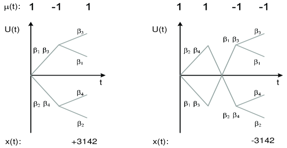
Figure 15: The shortest (left) and longest (right) scenario of the initial phase for $m=1$ and $\mu(0)=1$.

The first scenario is relatively easy to follow and we focus on the second one. The initial value is $\mu(0)=1$ and all strategies have the same utility $U=0$. Each agent at $t=0$ draws one strategy randomly. Let us assume that most of them decide to use the strategy suggesting $a(0)=-1$. As a result (i) $\beta_{2}$ and $\beta_{4}$ get positive payoff and, (ii) the next history is $\mu=1$ (cf. Tab. 1). After $\mu=1$ both winning strategies suggest the same action and lose. So the next history is $\mu=-1$. Since the history changed, the glued strategies have to react differently because two different $\mu$’s cannot cause the same reaction of all strategies. Thus, the longest time to split all $U$ trajectories is $2^{m+1}$ and requires every possible history to appear twice.

4.3.2 The concept of the state

At any step of the game one can rank all pairwise different strategies as the best, second best, third best, etc. Sizes of fractions corresponding to these strategies are known [17, 18]. An ordered list of indexes of different strategies, complemented by $\mu$ value, is sufficient to fully describe the game at a given moment and can be used as a characteristics of the state. Formally, assume $\{\beta_{\kappa}\}_{\kappa=1}^{2^{P}}$ is the set of pairwise different strategies indexed arbitrarily. There exists the sorting operator $\omega(\kappa)\rightarrow l$, ordering strategies according to their utilities, such that $l_{\beta_{k}}$ stands for the position of the strategy $\beta_{\kappa}$ in the ordered list. Then the state is as follows

$$x(t)=[\,\mu(t),l_{\beta_{1}}(t),\ldots,l_{\beta_{2^{P}}}(t)\,].$$ (50)

The total number of states is equal to $P\,\prod_{\kappa=0}^{2^{P}/2-1}(2^{P}-2\kappa)$ and accounts for all possible orders of $P$ strategies, provided each strategy has its anti-strategy , where the pair consisting of the strategy and its anti-strategy is characterized by the normalized Hamming distance equal to one.

As prevalent number of strategies have unique utility, the probability (20) for the active strategy $\alpha_{n}^{\prime}$ can be simplified (cf. also Ref. [17])

$$Pr\big{[}U_{\alpha_{n}^{\prime}}(t)=u_{l}\big{]}=\Big{(}1-\frac{l-1}{2^{P}}\Big{)}^{S}-\Big{(}1-\frac{l}{2^{P}}\Big{)}^{S},\quad\quad l\geq 1.$$ (51)

As a result, in the limit $N\rightarrow\infty$ about $N\;Pr\big{[}U_{\alpha_{n}^{\prime}}(t)=u_{l}\big{]}$ agents use the $l$-th best strategy. Subsequently, analysis of actions of strategies provides values of the aggregate demand in each state. Consider, for example, the case when $A$ is the largest possible. Since $\{u_{l}\}$ is a sorted list of utilities, this is possible if the first $l/2$ strategies in this list suggest actions opposite to the last $l/2$. Then the probability of an action suggested by the best strategy is equal to

$$Pr\big{[}a_{\alpha_{n}^{\prime}(t)}=a_{\alpha^{B}(t)}\big{]} = \sum_{l=1}^{2^{P-1}}Pr\big{[}U_{\alpha_{n}^{\prime}(t)}=u_{l}\big{]}$$ (52)

$$= 1-\frac{1}{2^{S}}.$$

This means that for large $NS$ for about $N(1-\frac{1}{2^{S}})$ agents their active strategy is the same as the best strategy and the absolute value of the aggregated demand is equal to

$$|A|=N\Big{(}1-\frac{1}{2^{S-1}}\Big{)}.$$ (53)

In particular, if $S=2$ then $|A|=N/2$.

4.3.3 De Bruijn representation

We know that $U$ trajectories represent mean-reverting processes. Thus, the state space (50) is projected onto the subspace $x(t)=\,\mu(t)$ and the dynamics of the MG can be efficiently studied using de Bruijn graphs, as shown in Ref. [24]. The decision history $\mu(t)$ is a sequence of $m$ minority actions

$$\mu(t)=\big{[}a^{\ast}(t-m),a^{\ast}(t-m+1),\ldots,a^{\ast}(t-1)\big{]}.$$ (54)

The $\mu(t+1)$ is obtained by adding $a^{\ast}(t)$ to the right and deleting $a^{\ast}(t-m)$ from the left of the vector (54), such that there are two possible successors $\mu(t+1)$ of $\mu(t)$. If one history can be obtained from another one using this procedure, then the latter has a directed edge to the former one. Histories may be represented by labelled edges. These rules define de Bruijn graph of the order $m$. Examples for $m=1$ and $m=2$ are given in Figs 16.

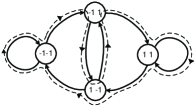
Figure 16: De Bruijn graphs of orders $m=1$ (left) and $m=2$ (right). Dashed lines represent examples of the Euler trails on the graph: one trail for $m=1$ (left) and one of two possible Euler trails for $m=2$ (right)

Histories in MGs are not equiprobable [24]. Among all paths on the de Bruijn graph of the game, Euler paths define the shortest sequence of histories where each strategy loses and wins equally likely. In the non-Eulerian paths some histories are more frequent and therefore some strategies are more profitable. We show in the following that in the efficient mode the non-Eulerian paths are rare compared to the Eulerian ones.

4.3.4 Algorithm generating strong demand fluctuations

We noticed that large fluctuation of $A$ is only possible if the game is in one of two de Bruijn nodes called homogeneous, i.e. consisting of identical symbols: $\mu_{h1(2)}=\big{[}-(+)1,\ldots,-(+)1\big{]}$. Interesting enough, peaks are observable only after one of the homogenous histories, but not after both. In Fig. 17 we present the flow chart illustrating appearance of strong fluctuations of $A(t)$.

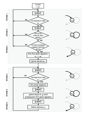
Figure 17: The flow chart of the MG evolution algorithm, illustrating appearance of distinct peaks of demand.

Below we describe the algorithm step by step. First three stages lead to the first peak. Next steps explain why the subsequent peaks follow each other and why they have opposite signs.

• If $A(t_{1})$ stands for the first peak of demand then three prior conditions have to be fulfilled. The first is that $\mu(t_{1}-1)=\mu_{h1(2)}$, where $\mu_{h1(2)}=[-(+)1,\ldots,-(+)1]$ is a homogeneous node.

• It is also required that at $t_{1}-1$ majority of agents decides to change the node. If this is fulfilled then the minority action is

  $$a^{\ast}(t_{1}-1)=\left\{\begin{array}[]{rr}-1,&\quad\mu(t_{1}-1)=\mu_{h1}\\ 1,&\quad\mu(t_{1}-1)=\mu_{h2}\end{array}\right..$$ (57)

  Hence $\mu(t_{1})=\mu(t_{1}-1)$, the minority action is to stay in the same node and gives the positive payoff to the winning strategy

  $$R_{\alpha_{n}^{s}}(t_{1}-1)=-a_{\alpha_{n}^{s}}A(t_{1}-1).$$ (58)

  
  

• There is a non-zero probability that strategies corresponding to the first $l/2$ utilities in $\{u_{l}\}$ have won in the last step. Such circumstance is possible provided stages 1 and 2 are realized. If this third condition is fulfilled then we mark such history $\mu_{C}$. Then all first $l/2$ strategies suggest the same reaction after $\mu_{C}$. Hence the majority decision at $t_{1}$ is to stay in the node and the maximal demand (cf. Eq. (52)) is generated. All strategies with high utility get the penalty and the low-utility ones are rewarded by the same amount. The game follows the minority decision and escapes from the de Bruijn node $\mu_{C}$. When the game leaves $\mu_{C}$, the strategy set is split into two groups of high and low utility, as illustrated in Fig. 18. In the next steps the game goes to $\mu\neq\mu_{C}$.

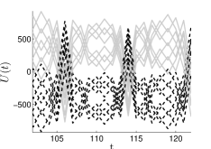
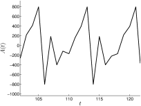
  Figure 18: The time evolution of the utilities (left) and the aggregated demand (right) for the MG with $N=1601$, $S=2$, $m=2$ and $g(x)=x$. Grey solid trajectories represent strategies reacting in the same way after particular history $\mu_{C}$. Black dashed trajectories represent anti-correlated strategies reacting in the opposite way after $\mu_{C}$. The appearance of $\mu_{C}$ is in $t=105$ and $106$ and then after every $2^{m+1}$ steps.

• Next steps do not substantially affect utilities as long as the history $\mu_{C}$ does not reappear. There is no history other than $\mu_{C}$ assuring that the first $l/2$ strategies in the $\{u_{l}\}$ list suggest a collective action resulting with the most spiky demand. Hence, after $t_{1}$, the variations of $A$ do not affect the utility significantly until the $\mu_{C}$ reappears at $t_{2}>t_{1}$ and when the set of the best $l/2$ strategies is the same as at $t_{1}$. Then the $l/2$ best strategies suggest the game to shift to another node characterized by history $\mu(t_{2}+1)\neq\mu_{C}$ and the maximal demand $|A(t_{2})|=N(1-\frac{1}{2^{S-1}})$ is generated. All the $l/2$ best strategies get penalty proportional to the absolute value of the aggregated demand. Concurrently, the $l/2$ strategies with the lowest utility are rewarded with the same amount (cf. Fig. 18).

• Next, the game follows the edge leading to the same node. Subsequently, the $l/2$ best strategies suggest staying in the same vertex $\mu_{C}$. Again, high absolute value of demand is generated but the sign of $A(t_{2}+1)$ is opposite to the sign of $A(t_{2})$. Consequently, all strategies with high $U(t_{2}+1)$ get penalty $N(1-\frac{1}{2^{S-1}})$ and, concurrently, strategies with low utility get reward of the same size.

• The game goes to the vertex $\mu_{C}(t_{2}+2)\neq\mu_{C}$ and stages 4–6 repeat.

Since high $A(t)$ appears only after the history $\mu_{C}$, we have just two transitions in the Eulerian path starting from this history. From this it follows that the frequency of peaks is equal to

$$f = \frac{2}{2^{m+1}}$$ (59)

$$= \frac{1}{2^{m}},$$

in agreement with our simulations. The value $2^{m+1}$ is the length of the Euler path and it corresponds to the period of $A$ observed in Figs. 9-9.

4.3.5 The Markov process representation

The case of equal-size fractions

As pointed out in Sec. 4.2, rewards and penalties have to compensate if the game is stable. This requires specific order of states (cycle), such that every $\mu$ has to appear twice over the cycle, in order to assure the same magnitudes of reward and penalty for any strategy. Such cycles are considered as attractors because, as we will see, they tend to pull in other initial states. The question is: how many attractors exist and how one can find them? At least two ways of dealing with the problem are possible for equal-size fractions. The first is a brute force method where for each state its successor is determined. But usefulness of this method is limited only to small $m$. Another approach requires analysis of the Euler paths on de Bruijn graph and is applicable for any $m$. We will show subsequently that the number of attractors is two times larger than the number of Euler paths. Below are examples of both methods.

We present the brute force method for $m=1$ and strategies defined as in Tab. 2. For simplicity, we use abridged notation for the state, e.g. $-3412$ stands for $[-1,3,4,1,2]$. Each state has to be analyzed and its successor has to be found. Fig. 19 presents relations between states. There are two attractors:

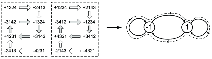
Figure 19: Two basins of attraction for $m=1$ (left). Attractors are marked by grey arrows. Both attractors are projected to the same Euler path in de Bruijn graph (right). For simplicity, we use abridged notation for the state, e.g. $-3412$ stands for $[-1,3,4,1,2]$.

Attractor 1 $$= [+4231,-3142,-1324,+3142]$$ (60)

Attractor 2 $$= [+4321,-3412,-1234,+3412]$$ (61)

Both attractors are equally possible, provided that $U(t=0)=\mbox{const}$ for all strategies. Each attractor assures that every possible history appears twice. One appearance rewards half of strategies and another one penalizes them. Each reward and subsequent penalty are of the same magnitude. Moving along attractors assures that the game follows the Euler trail in the de Bruijn graph, consistently with results of Refs. [5, 24]. An example of $U$ trajectories corresponding to these attractors is presented in Fig. 20.

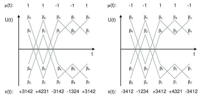
Figure 20: Utility trajectories for two possible attractors for $m=1$.

The absolute changes of utilities in analyzed case $m=1$ are equal to one of two values: $N/2$ or $N/4$, depending on state. In the former case, both best strategies suggest the same action. Thus the $3/4$ of population acts according to these actions and an aggregate demand is equal to $|A|=\frac{3}{4}N-\frac{1}{4}N=\frac{N}{2}$. In the latter case, the first and the third strategy suggest the same action. Hence, the $\frac{10}{16}$ of the population chooses the same action and consequently $|A|=\frac{10}{16}N-\frac{6}{16}N=\frac{N}{4}$. Exemplified realization for $m=1$ is shown in Fig. 21.

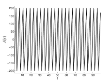
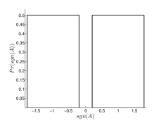
Figure 21: Time evolution of the aggregated demand $A(t)$, estimated $Pr(A)$ and $Pr(\mbox{sgn}(A))$ for the population size $N=400$, agent memory $m=1$, $S=2$ strategies per agent, identical sizes of fractions (reference system) and linear payoff $g(x)=x$

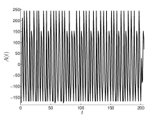
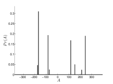
Figure 22: Time evolution of the aggregated demand ${A}(t)$, plots of the estimated $Pr({A})$ and $Pr(\mbox{sgn}({A}))$ for the population size $N=400$ and agent memory $m=1$, $S=2$ strategies per agent and unequal sizes of fractions.

It is seen that both distributions, $A$ and $\mbox{sgn}(A)$, are symmetric. Since the game is fully deterministic, each of four states $x_{1}\ldots x_{4}$ is related to only one value of $A(x)$. Hence, the $A$ distribution has four peaks.

More general way to determine the number of attractors is to count the number of Eulerian paths in de Bruijn graph. Each attractor consists of the unique set of states that do not appear in other attractors. We proved in Sec. 4.3.4 that each attractor comprises of exactly one state characterized by the large oscillation $|A|=N(1-\frac{1}{2^{S-1}})$. This state has to incorporate the $\mu$ representing one of the two possible homogenous nodes of the de Bruijn graph. As a consequence, there are two different states belonging to two different attractors where both attractors are projected on the same Eulerian path in de Bruijn graph. According to the theory of de Bruijn sequences, there is $2^{2^{m}}/2^{m+1}$ Eulerian paths [25]. Hence, there is twice that many attractors, $2^{2^{m}}/2^{m}$, e.g. there are $2,4$ and $32$ attractors for $m=1,2$ and $3$, respectively.

The case of unequal-size fractions

The size of different fractions most likely varies for strategies drawn randomly. This shifts the a posteriori ${A}$ distribution with respect to that of the reference system. The mechanism is the same as for the steplike payoff. Consequently, in each state belonging to the attractor, the values of $A$ are different than in the case of equal-size fractions. If the game follows an attractor, the $A$ would not compensate to zero along the path and the utility values would grow or shrink indefinitely. The minority mechanism stabilizes the game and prevents such scenario by adding states to the attractor. Exemplified realization for the case, where strategies are drawn from uniform distribution, is shown in Fig. 22. It is seen that both $Pr({A})$ and $Pr(\mbox{sgn}({A}))$ are asymmetric if distributions are considered a posteriori. The comparison of Markov chains, where sizes of fractions are equal and different, is shown in Fig. 23.

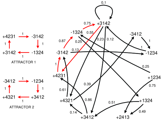
Figure 23: Two possible attractors for $m=1$ (left) for game with equal sizes of fractions. The transition graph for a real game where sizes are unequal, i.e. strategies are drawn from uniform distribution (right).

It is seen that the game with unequal fractions mostly follows attractor $1$ (red arrows) but in three of four states transitions to other states can appear either. The probability of these transitions is relatively small, indicating that sizes of fractions do not differ a lot. The MP representation for unequal fractions is different for each realization.

4.3.6 The variance per capita $\sigma^{2}/N$

We proved in Sec. 4.3.4 that large oscillations are periodic and equal to:

$$|A|=N\Big{(}1-\frac{1}{2^{S-1}}\Big{)}.$$ (62)

In particular, if $S=2$ then $\sigma^{2}\sim\frac{N^{2}}{4}$, consistently with observations and results of Ref. [17].

The argumentation in Sec. 4.3.4 becomes strict and Eq. (52) is exact in the efficient mode when $NS\gg 2^{P}$, ideally in the limit $NS\rightarrow\infty$. But we also observe cyclic peaks of demand for $N=1601$ and $m=5$, when the efficiency condition is not met (cf. Fig. 9, right). In fact, the condition $NS\gg 2^{P}$ can be slacken off to the requirement that the population is numerous enough that the game is in the herd mode. Games in that mode do not follow Eulerian paths because for smaller $N$ the pool of strategies is too sparse and some histories occur more frequently. Nevertheless, the mechanism of peak creation is approximately preserved, as long as $N$ is large enough to cause the split of utilities into two groups.

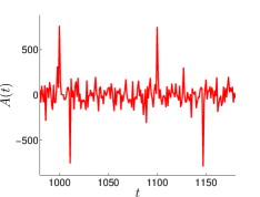
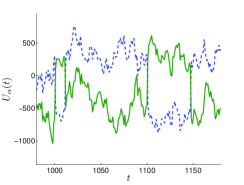
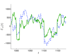
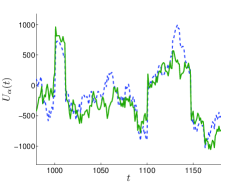
Figure 24: The time evolution of the aggregated demand (upper left) and utilities for three cases: an agent with one high- and one low-utility strategy (upper right), two low-utility strategies (lower left) and two high-utility strategies (lower right) at $t=1000$. These three cases may be quantitatively distinguished using the values of utilities at $t=1000$, corresponding to the location of the first maximum of $A(t)$ in the upper left panel. Simulation was performed for the MG with $N=1601$, $S=2$, $m=5$ and $g(x)=x$.

At any time a somewhat simpler explanation of large oscillations may be given by dividing strategies into two categories: the good with the positive payoff, and bad with negative. Probability that an agent has no good strategies, or at least one good, is equal to $\frac{1}{2^{S}}$ and $1-\frac{1}{2^{S}}$, respectively. Rapid fluctuations of demand are transferred to similar fluctuations of the utility. The $A(t_{1})$ fluctuates after the history $\mu_{C}=\mu(t_{1})$ when the strategies with higher utility indicate identical actions. If $A(t_{1})$ strongly fluctuates, then at $t_{1}+1$ about $N(1-\frac{1}{2^{S}})$ agents have at least one strategy with high utility and they choose it. Strategies split into two groups: the first group consisting of high utilities and the second of low utilities, with a gap between these two groups (cf. Fig. 18). Strategies with utilities belonging to the same group do not suggest the same actions, provided $\mu\neq\mu_{C}$, and therefore no peak of $A$ is generated. The $\mu_{C}$ has a non-vanishing probability to reappear at some $t_{2}>t_{1}$. All agents belonging to the group with at least one high-utility strategy tend to react identically and $A(t_{2})$ fluctuates maximally, i.e. $A(t_{2})=N(1-\frac{1}{2^{S-1}})$. This is illustrated in Fig. 24 (upper left), where for $S=2$ we have $A(t=1000)=\frac{N}{2}$. At $t_{2}$, all strategies with high $U(t_{2})$ fail and get the penalty $-A(t_{2})$, whereas those with low $U(t_{2})$ are rewarded with $A(t_{2})$. After $t_{1}$ agents are divided into three groups, provided $S=2$: the group with two good strategies, with one good and one bad, and with two bad. As seen in Fig. 24, at $t=1000$ a quarter of the population with two high-utility strategies evolves into two low-utility groups (lower left), and vice versa for another quarter with two initially low-utility strategies (lower right). Remaining half of the population just swaps utilities of their strategies (upper right).

Results showing periodicity of $A(t)$ from simulations become closer to the theoretical results for large $NS/2^{P}$ ratio. If this ratio is small, then the game hardly follows the Eulerian path and peaks of $A(t)$ appear randomly.

4.3.7 Stability of the game and behavior of the predictability $H$

The behavior of $H_{A}$ is driven by absolute disproportions between fractions’ sizes. The payoff is an explicit function of $A$ and, in order to stabilize the game, the negative and positive payoffs following the same $\mu$ have to compensate mutually. Hence, for any $\mu$: $\langle A^{-}|\mu\rangle=\langle A^{+}|\mu\rangle$ and $\langle H_{A}\rangle=0$. For this kind of payoff the same frequency of the negative and positive payoffs do not have to be preserved as it is required for $\mbox{sgn}(x)$ (see Fig. 22, bottom left).

The last point to understand is the plot of $H_{a}/N$ that seems to be equal to zero in the herd regime. The $H_{a}$ is the sum of $\langle a^{*}|\mu\rangle$ over $P$ different $\mu$’s. Each of these components is most likely nonzero and is bounded: $\langle a^{*}|\mu\rangle\in[-1,1]$. Thus $\mbox{max}(H_{a})=\mbox{const}=P$ and in the limit $N\rightarrow\infty$ one has $H_{a}/N=0$.

4.4 The effect of imbalance between fractions

One can try to measure how the size of disproportion between fractions affects transition probabilities in the Markov chain. To this end we incorporate a measure of the distance between two arbitrary processes. Denoting the set of reference processes by ${\cal R}$ and the set of examined ones by ${\cal E}$, this measure is defined as

$$\Upsilon=\sum_{i\in{\cal E\bigcup\cal R}}\sum_{j\in{\cal E\bigcup\cal R}}\big{|}Pr^{\cal E}(x_{i})Pr^{\cal E}(x_{j}|x_{i})-Pr^{\cal R}(x_{i})Pr^{\cal R}(x_{j}|x_{i})\big{|}.$$ (63)

where $Pr^{\cal R}$ and $Pr^{\cal E}$ stand for the probabilities for the reference and examined system. The $\Upsilon\in[0,2]$ is suitable to compare any MPs, comprising even such where processes are based on different sets of states. If $\Upsilon=0$, then there are no differences between processes. If $\Upsilon=2$, then processes are based on strongly disjunctive sets of states.

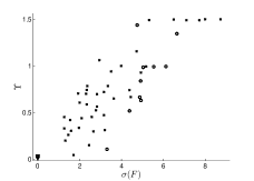
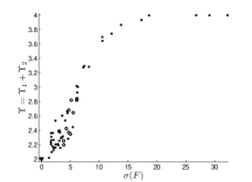
Figure 25: Distance $\Upsilon$ as a function of $\sigma(F)$ for two different payoffs $g(x)=\mbox{sgn}(x)$ (left) and $g(x)=x$ (right).

The standard deviation $\sigma(F)$ is a measure of disproportion of fractions. The $Upsilon$ as a function of $\sigma(F)$ is presented in Fig. 25. The left panel presents $\Upsilon$ measured between the reference MP (left-hand diagram in Fig. 13) and 40 games where strategies are drawn from various distributions, provided $g(x)=\mbox{sgn}(x)$. In the case $g(x)=x$, the function is more complicated because we do not have just one MP representing the reference system but for $m=1$ there are two equiprobable attractors, corresponding to two MPs. Therefore we use the sum of $\Upsilon_{1}+\Upsilon_{2}$ as a function of imbalance between fractions, as presented in Fig. 25 (right). If the game follows attractor 1 then $\Upsilon_{1}=0$ and $\Upsilon_{2}=2$.

5 Conclusions

In this paper we proposed a consistent, reductionist scheme explaining phenomenology of minority games in the efficient regime. In this mode the size of strategy space is much smaller than the number of strategies used by agents and the population as a whole can access complete information about the game.

Our discussion begun with the phenomenology. We considered a number of macroscopic random variables, or their moments, characterizing the game and being particularly important for applications, such as the aggregated demand, demand’s variance per capita and decision’s or demand’s predictabilities. We studied these variables as functions of the control parameters, e.g. the ratio of the total number of agents to the number of all possible winning histories, as well as their time evolution. Among interesting features we found that predictabilities may, or may not, be sensitive to the form of the payoff function, depending on how the predictabilities are actually defined: using winning decisions only or the overall demand.

Deeper insight into the mechanism of these behaviors was possible by performing coarse-graining and aggregation of some internal degrees of freedom of the game, thus defining an intermediate level of description, called mesoscopic. At such mesoscopic level, fractions of agents using same strategies are treated as separate entities. Using this method, in the efficient regime when $NS\gg 2^{P}$, we also managed to represent the game as a Markov process with the finite number of states.

In case where the Markov representation is known, two methodologies were proposed to explain our observations. First, in the simplified case, the quenched disorder was neglected, i.e. fractions were assumed to be equal size. In this case, however, not all observations are properly explained. Behavior of predictability required extended methodology where the quenched disorder was used. Two payoffs, the steplike and linear, were separately analyzed. We showed that in case of the steplike payoff, the stochastic and deterministic transitions were possible, whereas for the linear payoff, all transitions were deterministic.

We argued that the Markov process representation of the game completely defines and explains the dynamics of the game in the stationary regime, and allows for the calculation of state occupancies. If the transition probabilities in the Markov chain are known, the phenomenology also becomes understandable. For example, the Markov representation provides an explanation of the periodicity and preferred levels of the aggregate demand $A(t)$. In practical terms, this approach is tough for $m>1$ due to the large number of states but the whole reasoning remains valid in general. We failed to find any relation between the memory length $m$ and the total number of states.

Neither the simplified concept of state nor the Markov process description seem to be correct if the initial preference was given to any strategy. The definition of the stability was introduced in Sec. 4.1.3, in order to better understand asymmetries observed for aggregated variables. The stability mechanism appeared to be sensitive to the payoff function. In case the steplike payoff was considered, then the frequency of opposite signs of $A$ after any $\mu$ had to be preserved. In case of the linear payoff, the negative and positive values of A had to compensate mutually. As a result, depending on the payoff, both the $H_{a}$ and $H_{A}$ were equal to zero in the herd regime.

Differences between systems with equal-size fractions and those with unequal-size fractions were more likely for larger numbers of agents. This was particularly reflected in distortions of: (i) the transition probabilities, in case of the steplike payoff, and (ii) attractors, in case of the linear payoff. In order to quantify this distortion, the measure of distance between two Markov processes was introduced.

We studied games with the full, maximal strategy space. Some authors, e.g. in Refs. [2, 26], reduced the strategy space and reproduced many features of the full MG, e.g. behavior of variance per capita. The drawback of their method is that it reduces the number of states in the Markov-chain description of the game and significantly affects its time evolution. The Markov representation is oversimplified by such reduction.

Some observables for the proportional payoff were explained without using the Markov process. For example, there was an observation of distinct peaks of the aggregated demand, exhibiting height equal to a half of the population, assuming $S=2$. We showed that in the herd regime, there always exists a history $\mu_{C}$ for which the fraction $1-\frac{1}{2^{S}}$ of agents reacts identically and this is seen in the peak $A(t)=N(1-\frac{1}{2^{S-1}})$. Apart from using the Markov chain technique, we found another, simpler one, where only two classes of strategies were used instead of all $2^{P}$ classes. This technique is not limited to the case $NS\gg 2^{P}$ but works in the whole herd regime. This approach was also successfully exploited in our analysis of the multi-market minority game [27].

Considering further research, it could be a significant achievement if a single, closed-form equation were found for the entire parameter region of the MG. So far, in literature, such equations have indeed been found in the crowded and random regions separately. But a unified description of the entire range of parameters is still lacking.

References

- Arthur [1994] W. B. Arthur, Inductive reasoning, bounded rationality, and the bar problem, in: Am. Econ. Rev., volume 84, pp. 406 – 411.
- Challet and Zhang [1997] D. Challet, Y. Zhang, Emergence of cooperation and organization in an evolutionary game, in: Phys. A, volume 246, pp. 407 – 418.
- Challet and Zhang [1998] D. Challet, Y. Zhang, On the minority game: Analytical and numerical studies, in: Phys. A, volume 256, pp. 514 – 532.
- Challet et al. [2005] D. Challet, M. Marsili, Y.-C. Zhang, Minority Games, Oxford Univ. Press, New York, 2005.
- Jefferies et al. [2001] P. Jefferies, M. Hart, N. Johnson, Deterministic dynamics in the minority game, in: Phys. Rev. E, volume 65, pp. 016105 – 016113.
- Coolen [2005] A. Coolen, The mathematical theory of minority games: statistical mechanics of interacting agents, Oxford Univ. Press, 2005.
- Savit et al. [1999] R. Savit, R. Manuca, R. Riolo, Adaptive competition, market efficiency, and phase transitions, in: Phys. Rev. Lett., volume 82, pp. 2203 – 2206.
- de Cara et al. [1999] M. de Cara, O. Pla, F. Guinea, Competition, efficiency and collective behavior in the El Farol bar model, in: Eur. Phys. J. B, volume 10, pp. 187 – 191.
- Challet et al. [2000] D. Challet, M. Marsili, R. Zecchina, Statistical mechanics of heterogeneous agents: minority games, in: Phys. Rev. Lett., volume 84, pp. 1824 – 1827.
- Marsili et al. [2000] M. Marsili, D. Challet, R. Zecchina, Exact solution of a modified El Farol’s bar problem: Efficiency and the role of market impact, in: Phys. A, volume 280, pp. 522 – 553.
- Marsili and Challet [2001] M. Marsili, D. Challet, Continuum time limit and stationary states of the minority game, in: Phys. Rev. E, volume 64, p. 056138.
- Garrahan et al. [2000] J. P. Garrahan, E. Moro, D. Sherrington, Continuous time dynamics of the thermal minority game, in: Phys. Rev. E, volume 62, pp. R9 – R12.
- Heimel and Coolen [2001] J. Heimel, A. Coolen, Generating functional analysis of the dynamics of the bath minority game with random external information, in: Phys. Rev. E, volume 63, p. 056121.
- Johnson et al. [1999] N. F. Johnson, M. Hart, P. Hui, Crowd effects and volatility in in markets with competing agents, in: Phys. A, volume 269, pp. 1 – 8.
- Hart et al. [2001] M. Hart, P. Jefferies, N. Johnson, P. Hui, Crowd-anticrowd theory of the minority game, in: Phys. A, volume 298, pp. 537 – 544.
- Moro [2004] E. Moro, The minority game: an introductory guide, in: Adv. in Cond. Matt. and Stat. Phys., pp. 263 – 286.
- Hart et al. [2001] M. Hart, P. Jefferies, P. Hui, N. Johnson, Crowd-anticrowd theory of multi-agent market games, in: Eur. Phys. J. B, volume 20, pp. 547 – 550.
- Wawrzyniak and Wiślicki [2009] K. Wawrzyniak, W. Wiślicki, Phenomenology of minority games in efficient regime, in: Adv. in Comp. Sys., volume 12, pp. 619 – 639.
- Jefferies et al. [2001] P. Jefferies, M. Hart, P. Hui, N. Johnson, From market games to real-world markets, in: Eur. Phys. J. B, volume 20, pp. 493 – 501.
- Zheng and Wang [2001] D. Zheng, B.-H. Wang, Statistical properties of the attendance time series in the minority game, in: Phys. A, volume 301, pp. 560 – 566.
- Wawrzyniak [ence] K. Wawrzyniak, On Phenomenology, Dynamics and some Applications of the Minority Game, PhD dissertation, Institute of Computer Science, Polish Academy of Sciences, 2011 - submitted for defence.
- Challet and Marsili [1999] D. Challet, M. Marsili, Phase transition and symmetry breaking in the minority game, in: Phys. Rev. E, volume 60, pp. 6271 – 6274.
- Cavagna [1999] A. Cavagna, Irrelevance of memory in the minority game, in: Phys. Rev. E, volume 59, pp. R3783 – R3786.
- Challet and Marsili [2000] D. Challet, M. Marsili, Relevance of memory in minority games, in: Phys. Rev. E, volume 62, pp. 1862 – 1868.
- van Aardenne-Ehrenfest and de Bruijn [1951] T. van Aardenne-Ehrenfest, N. de Bruijn, Circuits and trees in oriented linear graphs, in: Simon Stevin, volume 28, pp. 203 – 217.
- Li et al. [2000] Y. Li, A. VanDeemen, R. Savit, The minority game with variable payoffs, in: Phys. A, volume 284, pp. 461 – 477.
- Wawrzyniak and Wiślicki [2009] K. Wawrzyniak, W. Wiślicki, Multi-market minority game: breaking the symmetry of choice, in: Adv. in Comp. Sys., volume 12, pp. 423 – 437.