Cooperative Beamforming for Dual-Hop Amplify-and-Forward Multi-Antenna Relaying Cellular Networks

Abstract

In this paper, linear beamforming design for amplify-and-forward relaying cellular networks is considered, in which base station, relay station and mobile terminals are all equipped with multiple antennas. The design is based on minimum mean-square-error criterion, and both uplink and downlink scenarios are considered. It is found that the downlink and uplink beamforming design problems are in the same form, and iterative algorithms with the same structure can be used to solve the design problems. For the specific cases of fully loaded or overloaded uplink systems, a novel algorithm is derived and its relationships with several existing beamforming design algorithms for conventional MIMO or multiuser systems are revealed. Simulation results are presented to demonstrate the performance advantage of the proposed design algorithms.

1 Introduction

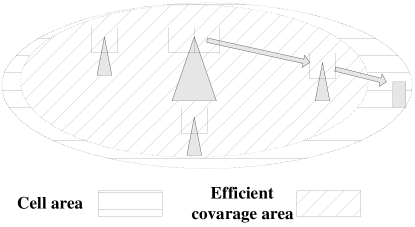
Figure 1: Amplify-and-forward MIMO relaying cellular network.

Cooperative communication is a promising technology to improve quality and reliability of wireless links [1, 2, 3, 4, 5, 6, 7, 8]. One of the most important application scenarios of cooperative communications is cellular network. Due to shadowing or deep fading of wireless channels, base station may not be able to sufficiently cover all mobile terminals in a cell, especially those on the edge. Deployment of relay stations is an effective and economic way to improve the communication quality in cellular networks, as shown in Fig. 1.

In cooperative cellular networks, there are two major strategies in relaying. Relay station can either decode the received signal before retransmission [9] or simply amplify-and-forward (AF) the received signal to the corresponding destination without decoding [10]. AF strategy has low complexity and minimal processing delay, and is more secure. These reasons make AF preferable in practical implementation. In fact, deployment of AF relay station with multiple antenna to enlarge coverage of base station is one of the most important components in the future communication protocols, e.g., LTE, IMT-Advanced and Winner project [11], [12].

With multiple antennas at mobile terminals, relay station and base station, a natural question is how to allocate limited power resource in the spatial domain. In general, power allocation is equivalent to beamforming matrices design at base station, relay and mobile terminals, and the objective can be maximizing capacity [13] or minimizing the mean-square error (MSE) of the recovered data [14]. The MSE criterion is a widely chosen one since it aims at the data be recovered as accurate as possible, and is extensively used in power allocation in classical point-to-point [15, 17, 16] or multi-user MIMO systems[18, 19, 20, 22, 21, 23, 24]. The MSE minimization is also related to capacity maximization [17], [22] if a suitable weighting is applied to different data streams.

In a cellular network, the base station and relay station are usually allowed to be equipped with multiple antennas. For each mobile terminal, if it is equipped with single antenna, such relay cellular networks has been investigated from various point-of-views. For example, beamforming design for capacity maximization has been considered in [9], and quality-of-service based power control has been investigated in [10]. However, in the next generation multi-media wireless communications, it is likely that the size of a mobile terminal allows multiple antennas to be deployed. Unfortunately, extension from the previous works on single antenna mobile terminals to multi-antenna terminals is by no mean straightforward.

In this paper, we take a step further to consider the case where each mobile terminal is also equipped with multiple antennas. In particular, we consider the joint precoders, forwarding matrix, and equalizers design for both uplink and downlink AF relaying cellular network, under power constraints. The design problems are formulated as optimization problem minimizing the sum MSE of multiple detected data streams. While extension of the presented algorithm to weighted MSE criterion is straightforward, we focus on sum MSE for notational clarity. The contribution of the paper is as follows. Firstly, in the downlink, the precoder at base station, forwarding matrix at relay station and equalizers at mobile terminals are jointly designed by an iterative algorithm. Secondly, in the uplink case, we demonstrate that the formulation of the beamforming design problem has the same form as that in the downlink, and the same iterative algorithm can be employed. Thirdly, since the general iterative solution provides little insight, we derive another algorithm under the specific case when the number of independent data streams from different mobile terminals is greater than or equal to their number of antenna. It is found that the resultant solution includes several existing algorithms for multi-user MIMO or AF relay network with single antenna as special cases.

The paper is organized as follows. In Section 2, beamforming design problem in downlink is investigated, and an iterative algorithm is presented. In Section 3, the analogy of the uplink and downlink beamforming design problems is demonstrated. Furthermore, another beamforming design algorithm is derived for the specific case of fully loaded or overloaded system, and the relationships of this algorithm with other existing algorithms are discussed. Simulation results are given in Section 4 to demonstrate the effectiveness of the proposed algorithms. Finally, conclusions are drawn in Section 5.

The following notations are used throughout this paper. Boldface lowercase letters denote vectors, while boldface uppercase letters denote matrices. The notation ${\bf{Z}}^{\rm{H}}$ denotes the Hermitian of the matrix ${\bf{Z}}$, and ${\rm{Tr}}({\bf{Z}})$ is the trace of the matrix ${\bf{Z}}$. The symbol ${\bf{I}}_{M}$ denotes an $M\times M$ identity matrix, while ${\bf{0}}_{M,N}$ denotes an $M\times N$ all zero matrix. The notation ${\bf{Z}}^{1/2}$ is the Hermitian square root of the positive semidefinite matrix ${\bf{Z}}$, such that ${\bf{Z}}^{1/2}{\bf{Z}}^{1/2}={\bf{Z}}$ and ${\bf{Z}}^{1/2}$ is also a Hermitian matrix. The operation ${\rm{diag}}\{[{\bf{A}}\ {\bf{B}}]\}$ is defined as a block diagonal matrix with ${\bf{A}}$ and ${\bf{B}}$ as block diagonal. The symbol ${\mathbb{E}}\{\bullet\}$ represents the statistical expectation. The operation ${\rm{vec}}({\bf{Z}})$ stacks the columns of the matrix ${\bf{Z}}$ into a single vector. The symbol $\otimes$ denotes the Kronecker product. For two Hermitian matrices, ${\bf{C}}\succeq{\bf{D}}$ means that ${\bf{C}}-{\bf{D}}$ is a positive semi-definite matrix.

2 Downlink Beamforming Design

2.1 System model and problem formulation

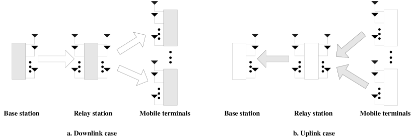
Figure 2: Amplify-and-forward MIMO relaying downlink and uplink cellular systems.

On the boundary of a cell, due to shadowing or deep fading, the direct link between base station (BS) and mobile terminals may not be good enough to maintain normal communication. Then mobile terminals will rely on relay station to communicate with BS. As shown in Fig. 2a, in downlink, signal is first transmitted from the BS to the relay station and then the relay station forwards the received signal to the corresponding mobile terminals. It is assumed that the BS has $N_{B}$ antennas and the relay station has $N_{R}$ antennas. For the $k^{\rm{th}}$ mobile terminal, it has $N_{M,k}$ antennas. The BS needs to simultaneously communicate with $K$ mobile terminals via a single relay station. There are $L_{k}$ data streams to be transmitted from the BS to the $k^{\rm{th}}$ mobile terminal, and the signal for the $k^{\rm{th}}$ mobile terminal is denoted by a $L_{k}\times 1$ vector ${\bf{s}}_{k}$. It is assumed that different data streams are independent, i.e., $\mathbb{E}\{{\bf{s}}_{k}{\bf{s}}_{j}^{\rm{H}}\}={\bf{0}}_{L_{k},L_{j}}$ when $k\neq j$ and $\mathbb{E}\{{\bf{s}}_{k}{\bf{s}}_{k}^{\rm{H}}\}={\bf{I}}_{L_{k}}$. With separate precoder ${\bf{T}}_{k}$ for different mobile terminals, the received signal at the relay station is

$${\bf{r}}={\bf{H}}_{BR}{\bf{T}}{\bf{s}}+{\boldsymbol{\eta}},$$ (1)

where ${\bf{H}}_{BR}$ denotes the $N_{B}\times N_{R}$ channel matrix between the BS and relay station, ${\bf{T}}=[{\bf{T}}_{1},\ \cdots,\ {\bf{T}}_{K}]$, ${\bf{s}}=[{\bf{s}}_{1}^{\rm{T}},\ \cdots,\ {\bf{s}}_{K}^{\rm{T}}]^{\rm{T}}$ and the vector ${\boldsymbol{\eta}}$ denotes the additive Gaussian noise with zero mean and covariance matrix ${\bf{R}}_{{\boldsymbol{\eta}}}$. The power constraint at the BS is given by $\sum_{k}{\rm{Tr}}({\bf{T}}_{k}{\bf{T}}_{k}^{\rm{H}})\leq P_{s}$, where $P_{s}$ is the maximum transmit power.

At the relay station, before retransmission the signal ${\bf{r}}$ is multiplied with a forwarding matrix ${\bf{W}}$ under a power constraint ${\rm{Tr}}({\bf{W}}{\bf{R}}_{{\bf{r}}}{\bf{W}})^{\rm{H}}\leq P_{r}$, where $P_{r}$ is the maximum transmit power at the relay station and ${\bf{R}}_{{\bf{r}}}$ is the covariance matrix of the received signal ${\bf{r}}$:

$${\bf{R}}_{\bf{r}} ={\bf{H}}_{BR}{\bf{T}}{\bf{T}}^{\rm{H}}{\bf{H}}_{BR}^{\rm{H}}+{\bf{R}}_{{\boldsymbol{\eta}}}.$$ (2)

Finally, at the $k^{\rm{th}}$ mobile terminal, the received signal ${\bf{y}}_{k}$ is

$${\bf{y}}_{k}={\bf{H}}_{RM,k}{\bf{W}}{\bf{H}}_{BR}{\bf{T}}{\bf{s}}+{\bf{H}}_{RM,k}{\bf{W}}{\boldsymbol{\eta}}+{\bf{v}}_{k},$$ (3)

where matrix ${\bf{H}}_{RM,k}$ is the $N_{R}\times N_{M,k}$ channel matrix between the relay station and the $k^{\rm{th}}$ mobile terminal, and ${\bf{v}}_{k}$ is the additive Gaussian noise at the $k^{\rm{th}}$ mobile terminal with zero mean and covariance matrix ${\bf{R}}_{{\bf{v}}_{k}}$.

At each mobile terminal, an equalizer ${\bf{G}}_{k}$ is employed to detect the data. The mean-square-error (MSE) of data detection at the $k^{\rm{th}}$ terminal is

$${\rm{MSE}}_{k}({\bf{G}}_{k},{\bf{W}},{\bf{T}}_{k})$$ (4)

$$={\mathbb{E}}\{\|{\bf{G}}_{k}{\bf{y}}_{k}-{\bf{s}}_{k}\|^{2}\}$$

$$={\rm{Tr}}({\bf{G}}_{k}({\bf{H}}_{RM,k}{\bf{W}}{\bf{R}}_{{\bf{r}}}{\bf{W}}^{\rm{H}}{\bf{H}}_{RM,k}^{\rm{H}}+{\bf{R}}_{{\bf{v}}_{k}}){\bf{G}}_{k}^{\rm{H}})-{\rm{Tr}}({\bf{G}}_{k}{\bf{H}}_{RM,k}{\bf{W}}{\bf{H}}_{BR}{\bf{T}}_{k})$$

$$-{\rm{Tr}}(({\bf{G}}_{k}{\bf{H}}_{RM,k}{\bf{W}}{\bf{H}}_{BR}{\bf{T}}_{k})^{\rm{H}})+{\rm{Tr}}({\bf{I}}_{L_{k}}).$$ (5)

Now defining ${\bf{y}}=[{\bf{y}}_{1}^{\rm{T}},\ \cdots,\ {\bf{y}}_{K}^{\rm{T}}]^{\rm{T}}$, ${\bf{H}}_{RM}=[{\bf{H}}_{RM,1}^{\rm{T}},\ \cdots,\ {\bf{H}}_{RM,K}^{\rm{T}}]^{\rm{T}}$, ${\bf{v}}=[{\bf{v}}_{1}^{\rm{T}},\ \cdots,\ {\bf{v}}_{K}^{\rm{T}}]^{\rm{T}}$, and ${\bf{G}}={\rm{diag}}\{[{\bf{G}}_{1},\ \cdots,\ {\bf{G}}_{K}]\}$, the sum MSE can be written as

$${\rm{{MSE}}}_{D}({\bf{G}},{\bf{W}},{\bf{T}})= \sum_{k=1}^{K}{\rm{MSE}}_{k}({\bf{G}}_{k},{\bf{W}},{\bf{T}}_{k})$$

$$= {\rm{Tr}}({\bf{G}}({\bf{H}}_{RM}{\bf{W}}{\bf{R}}_{{\bf{r}}}{\bf{W}}^{\rm{H}}{\bf{H}}_{RM}^{\rm{H}}+{\bf{R}}_{{\bf{v}}}){\bf{G}}^{\rm{H}})-{\rm{Tr}}({\bf{G}}{\bf{H}}_{RM}{\bf{W}}{\bf{H}}_{BR}{\bf{T}})$$

$$-{\rm{Tr}}(({\bf{G}}{\bf{H}}_{RM}{\bf{W}}{\bf{H}}_{BR}{\bf{T}})^{\rm{H}})+{\rm{Tr}}({\bf{I}}_{L}),$$ (6)

where $L=\sum_{k=1}^{K}L_{k}$ and ${\bf{R}}_{{\bf{v}}}={\rm{diag}}\{[{\bf{R}}_{{\bf{v}}_{1}},\ \cdots,\ {\bf{R}}_{{\bf{v}}_{K}}]\}$.

Therefore, the downlink beamforming optimization problem can be formulated as

$${\min_{{\bf{G}},{\bf{W}},{\bf{T}}}}\ \ \ \ \ {\rm{{MSE}}}_{D}({\bf{G}},{\bf{W}},{\bf{T}})$$

$$\ \ {\rm{s.t.}}\ \ \ \ \ \ {\rm{Tr}}({\bf{T}}{\bf{T}}^{\rm{H}})\leq P_{s}$$

$$\ \ \ \ \ \ \ \ \ \ \ \ {\rm{Tr}}({\bf{W}}{\bf{R}}_{{\bf{r}}}{\bf{W}}^{\rm{H}})\leq P_{r}$$

$$\ \ \ \ \ \ \ \ \ \ \ \ {\bf{G}}={\rm{diag}}\{[{\bf{G}}_{1},\ \cdots,\ {\bf{G}}_{K}]\}.$$ (7)

The optimization problem (2.1) is a nonconvex optimization problem for ${\bf{T}}$, ${\bf{W}}$ and ${\bf{G}}$, and there is no closed-form solution. This challenge remains even for the special case of multiuser MIMO systems [18], [19], [23] where only single hop transmission is involved. However, notice that when two out of the three variables are fixed, the optimization problem (2.1) for the remaining variable is a convex problem, and thus can be solved. Therefore, an iterative algorithm alternating the design of three variables can be employed.

2.2 Proposed iterative algorithm

(1) Equalizer design at the destination

When ${\bf{T}}$ and ${\bf{W}}$ are fixed, the optimization problem (2.1) is an unconstrained convex quadratic optimization problem for ${\bf{G}}$. Furthermore, since the structure of ${\bf{G}}$ is block diagonal, the design of individual ${\bf{G}}_{k}$ are decoupled. Therefore, the necessary and sufficient condition for the optimal solution is

$$\frac{\partial\sum_{k}{\rm{MSE}}_{k}({\bf{G}}_{k},{\bf{W}},{\bf{T}}_{k})}{\partial{\bf{G}}_{k}^{*}}={\bf{0}}_{L_{k},N_{M,k}},$$ (8)

and the optimal equalizer for the $k^{\rm{th}}$ mobile terminal can be easily shown to be

$${\bf{G}}_{k}=({\bf{H}}_{RM,k}{\bf{W}}{\bf{H}}_{BR}{\bf{T}}_{k})^{\rm{H}}({\bf{H}}_{RM,k}{\bf{W}}{\bf{R}}_{{\bf{r}}}{\bf{W}}^{\rm{H}}{\bf{H}}_{RM,k}^{\rm{H}}+{\bf{R}}_{{\bf{v}}_{k}})^{-1}.$$ (9)

(2) Forwarding matrix design at the relay station

When ${\bf{T}}$ and ${\bf{G}}$ are fixed, the optimization problem (2.1) is a constrained convex optimization problem for the variable ${\bf{W}}$, and the Karush-Kuhn-Tucker (KKT) conditions are the necessary and sufficient conditions for the optimal solution [25]. The KKT conditions of the optimization problem (2.1) with respective to ${\bf{W}}$ are [26]

$${\bf{H}}_{RM}^{\rm{H}}{\bf{G}}^{\rm{H}}{\bf{G}}{\bf{H}}_{RM}{\bf{W}}{\bf{R}}_{{\bf{r}}}+\lambda{\bf{W}}{\bf{R}}_{{\bf{r}}}=({\bf{H}}_{BR}{\bf{T}}{\bf{G}}{\bf{H}}_{RM})^{\rm{H}}$$ (10)

$$\lambda({\rm{Tr}}({\bf{W}}{\bf{R}}_{{\bf{r}}}{\bf{W}}^{\rm{H}})-P_{r})=0,\ \ \ \lambda\geq 0,$$ (11)

$${\rm{Tr}}({\bf{W}}{\bf{R}}_{{\bf{r}}}{\bf{W}}^{\rm{H}})\leq P_{r},$$ (12)

where $\lambda$ is the Lagrange multiplier.

Based on the first KKT condition (10), the optimal forwarding matrix ${\bf{W}}$ can be written as

$${\bf{W}} =({\bf{H}}_{RM}^{\rm{H}}{\bf{G}}^{\rm{H}}{\bf{G}}{\bf{H}}_{RM}+\lambda{\bf{I}})^{-1}({\bf{H}}_{BR}{\bf{T}}{\bf{G}}{\bf{H}}_{RM})^{\rm{H}}{\bf{R}}_{{\bf{r}}}^{-1},$$ (13)

where the value of $\lambda$ is computed using (11) and (12). Since $\lambda$ also appears in ${\bf{W}}$, (11) and (12) depends on $\lambda$ in a nonlinear way and there is no closed-form solution. Below, we propose a low complexity method to solve (11) and (12).

First, notice that in order to have (11) satisfied, either $\lambda=0$ or ${\rm{Tr}}({\bf{W}}{\bf{R}}_{{\bf{r}}}{\bf{W}}^{\rm{H}})=P_{r}$ must hold. If $\lambda=0$ also makes (12) satisfied, $\lambda=0$ is a solution to (11) and (12). On other hand, if $\lambda=0$ does not make (12) satisfied, we have to solve ${\rm{Tr}}({\bf{W}}{\bf{R}}_{{\bf{r}}}{\bf{W}}^{\rm{H}})=P_{r}$. It can be proved that [27] when ${\bf{T}}$ and ${\bf{G}}$ are fixed, the function $f(\lambda)={\rm{Tr}}({\bf{W}}{\bf{R}}_{{\bf{r}}}{\bf{W}}^{\rm{H}})$ is a decreasing function of ${\lambda}$ and the range of ${\lambda}$ must be within

$$0\leq\lambda\leq\sqrt{\frac{{\rm{Tr}}({\bf{E}}{\bf{R}}_{{\bf{r}}}^{-1}{\bf{E}}^{\rm{H}})}{P_{r}}}$$ (14)

where ${\bf{E}}=\sum_{k}\{({\bf{H}}_{BR}{\bf{T}}_{k}{\bf{G}}_{k}{\bf{H}}_{RM,k})^{\rm{H}}\}$. Therefore, $\lambda$ can be efficiently computed by one-dimension search, such as bisection search or golden search. Since ${\rm{Tr}}({\bf{W}}{\bf{R}}_{\bf{r}}{\bf{W}}^{\rm{H}})=P_{r}$ is a stronger condition than ${\rm{Tr}}({\bf{W}}{\bf{R}}_{\bf{r}}{\bf{W}}^{\rm{H}})\leq P_{r}$, (12) is satisfied automatically in this case. In summary, $\lambda$ is computed as

$$\lambda=\begin{cases}0&\text{if $f(0)\leq P_{r}$}\\ \text{Solve $f(\lambda)=P_{r}$ using bisection algorithm}&\text{Otherwise}\end{cases}.$$ (15)

(3) Precoder design at the BS

When ${\bf{W}}$ and ${\bf{G}}$ are fixed, the optimization problem (2.1) can be straightforwardly formulated as the following convex quadratic optimization problem for the precoder ${\bf{T}}$

$${\min_{{\bf{T}}}}\ \ \ {\rm{Tr}}({\bf{N}}_{0}^{\rm{H}}{\bf{T}}^{\rm{H}}{\bf{A}}_{0}{\bf{T}}{\bf{N}}_{0})+2\mathcal{R}\{{\rm{Tr}}({\bf{B}}_{0}^{\rm{H}}{\bf{T}})\}+c_{0}$$

$${\rm{s.t.}}\ \ \ \ {\rm{Tr}}({\bf{N}}_{1}^{\rm{H}}{\bf{T}}^{\rm{H}}{\bf{A}}_{1}{\bf{T}}{\bf{N}}_{1})+2\mathcal{R}\{{\rm{Tr}}({\bf{B}}_{1}^{\rm{H}}{\bf{T}})\}+c_{1}\leq 0,$$

$$\ \ \ \ \ \ \ \ {\rm{Tr}}({\bf{N}}_{2}^{\rm{H}}{\bf{T}}^{\rm{H}}{\bf{A}}_{2}{\bf{T}}{\bf{N}}_{2})+2\mathcal{R}\{{\rm{Tr}}({\bf{B}}_{2}^{\rm{H}}{\bf{T}})\}+c_{2}\leq 0,$$ (16)

where the corresponding parameters are defined as

$${\bf{A}}_{0} ={\bf{H}}_{BR}^{\rm{H}}{\bf{W}}^{\rm{H}}{\bf{H}}_{RM}^{\rm{H}}{\bf{G}}^{\rm{H}}{\bf{G}}{\bf{H}}_{RM}{\bf{W}}{\bf{H}}_{BR},\ \ \ {\bf{A}}_{1}={\bf{I}},\ \ \ {\bf{A}}_{2}={\bf{H}}_{BR}^{\rm{H}}{\bf{W}}^{\rm{H}}{\bf{W}}{\bf{H}}_{BR},$$

$${\bf{B}}_{0}^{\rm{H}} =-{\bf{G}}{\bf{H}}_{RM}{\bf{W}}{\bf{H}}_{BR},\ \ \ \ \ \ \ \ \ \ \ \ \ \ \ \ \ \ \ \ \ \ {\bf{B}}_{1}={\bf{B}}_{2}={\bf{0}},$$

$${\bf{N}}_{0} ={\bf{N}}_{1}={\bf{N}}_{2}={\bf{I}}_{L},$$

$$c_{0} ={\rm{Tr}}({\bf{R}}_{{\boldsymbol{\eta}}}{\bf{W}}^{\rm{H}}{\bf{H}}_{RM}^{\rm{H}}{\bf{G}}^{\rm{H}}{\bf{G}}{\bf{H}}_{RM}{\bf{W}})+{\rm{Tr}}({\bf{I}}_{L})+{\rm{Tr}}({\bf{G}}{\bf{R}}_{{\bf{v}}}{\bf{G}}^{\rm{H}}))$$

$$c_{1} =-P_{s},\ \ \ c_{2}={\rm{Tr}}({\bf{W}}{\bf{R}}_{{\boldsymbol{\eta}}}{\bf{W}}^{\rm{H}})-P_{r}.$$ (17)

Notice that the objective function and the constraints are of the same form. Using the property ${\rm{Tr}}({\bf{A}}{\bf{B}})={\rm{vec}}^{\rm{H}}({\bf{A}}^{\rm{H}}){\rm{vec}}({\bf{B}})$ and the property of Kronecker product, we can write $(l=0,1,2)$

$${\rm{Tr}}({\bf{N}}_{l}^{\rm{H}}{\bf{T}}^{\rm{H}}{\bf{A}}_{l}{\bf{T}}{\bf{N}}_{l})= {\rm{Tr}}({\bf{N}}_{l}^{\rm{H}}{\bf{T}}^{\rm{H}}{\bf{A}}_{l}^{\frac{\rm{H}}{2}}{\bf{A}}_{l}^{\frac{1}{2}}{\bf{T}}{\bf{N}}_{l})$$

$$= {\rm{vec}}^{\rm{H}}({\bf{A}}_{l}^{\frac{1}{2}}{\bf{T}}{\bf{N}}_{l}){\rm{vec}}({\bf{A}}_{l}^{\frac{1}{2}}{\bf{T}}{\bf{N}}_{l})$$

$$= {\rm{vec}}^{\rm{H}}({\bf{T}})({\bf{N}}_{l}^{*}\otimes{\bf{A}}_{l}^{\frac{\rm{H}}{2}})({\bf{N}}_{l}^{\rm{T}}\otimes{\bf{A}}_{l}^{\frac{1}{2}}){\rm{vec}}({\bf{T}}),$$ (18)

where the first equality is based on the fact that ${\bf{A}}_{l}$’s are positive semidefinite matrices. Furthermore, we can also write ${\rm{Tr}}({\bf{B}}_{l}^{\rm{H}}{\bf{T}})={\rm{vec}}^{\rm{H}}({\bf{B}}_{l}^{\rm{H}}){\rm{vec}}({\bf{T}})$. Putting these two results into (2.2) and after introducing an auxiliary variable $t$ [28], (2.2) is equivalent to the following optimization problem

$${\min_{{\bf{T}},t}}\ \ \ t$$

$${\rm{s.t.}}\ \ \ \ {\rm{vec}}^{\rm{H}}({\bf{T}})({\bf{N}}_{0}^{*}\otimes{\bf{A}}_{0}^{\frac{\rm{H}}{2}})({\bf{N}}_{0}^{\rm{T}}\otimes{\bf{A}}_{0}^{\frac{1}{2}}){\rm{vec}}({\bf{T}})\leq t-2\mathcal{R}\{{\rm{vec}}^{\rm{H}}({\bf{B}}_{0}^{\rm{H}}){\rm{vec}}({\bf{T}})\}$$

$$\ \ \ \ \ \ \ \ {\rm{vec}}^{\rm{H}}({\bf{T}})({\bf{N}}_{1}^{*}\otimes{\bf{A}}_{1}^{\frac{\rm{H}}{2}})({\bf{N}}_{1}^{\rm{T}}\otimes{\bf{A}}_{1}^{\frac{1}{2}}){\rm{vec}}({\bf{T}})\leq-c_{1}-2\mathcal{R}\{{\rm{vec}}^{\rm{H}}({\bf{B}}_{1}^{\rm{H}}){\rm{vec}}({\bf{T}})\}$$

$$\ \ \ \ \ \ \ \ {\rm{vec}}^{\rm{H}}({\bf{T}})({\bf{N}}_{2}^{*}\otimes{\bf{A}}_{2}^{\frac{\rm{H}}{2}})({\bf{N}}_{2}^{\rm{T}}\otimes{\bf{A}}_{2}^{\frac{1}{2}}){\rm{vec}}({\bf{T}})\leq-c_{2}-2\mathcal{R}\{{\rm{vec}}^{\rm{H}}({\bf{B}}_{2}^{\rm{H}}){\rm{vec}}({\bf{T}})\}.$$ (19)

Since $c_{0}$ does not affect the optimization problem, it has been neglected in (2.2).

With the Schur complement lemma [32], the optimization problem (2.2) can be further reformulated as the following semi-definite programming (SDP) problem [28]

$${\min_{{\bf{T}},t}}\ \ \ \ t$$

$${\rm{s.t.}}\ \ \left[{\begin{array}[]{*{20}c}{\bf{I}}&({\bf{N}}_{0}^{\rm{T}}\otimes{\bf{A}}_{0}^{\frac{1}{2}}){\rm{vec}}({\bf{T}})\\ (({\bf{N}}_{0}^{\rm{T}}\otimes{\bf{A}}_{0}^{\frac{1}{2}}){\rm{vec}}({\bf{T}}))^{\rm{H}}&-2\mathcal{R}\{{\rm{vec}}^{\rm{H}}({\bf{B}}_{0}){\rm{vec}}({\bf{T}})\}+t\\ \end{array}}\right]\succeq 0$$ (22)

$$\ \ \ \ \ \ \left[{\begin{array}[]{*{20}c}{\bf{I}}&({\bf{N}}_{l}^{\rm{T}}\otimes{\bf{A}}_{l}^{\frac{1}{2}}){\rm{vec}}({\bf{T}})\\ (({\bf{N}}_{l}^{\rm{T}}\otimes{\bf{A}}_{l}^{\frac{1}{2}}){\rm{vec}}({\bf{T}}))^{\rm{H}}&-2\mathcal{R}\{{\rm{vec}}^{\rm{H}}({\bf{B}}_{l}){\rm{vec}}({\bf{T}})\}-c_{l}\\ \end{array}}\right]\succeq 0,\ \ \ l=1,2.$$ (25)

The precoder at the BS is designed by solving this SDP problem using standard numerical algorithms such as interior-point polynomial algorithms [26], [28].

2.3 Summary and Initialization

In summary, the downlink beamforming matrices are computed iteratively. Since in each iteration, the MSE monotonically decreases, the iterative algorithm is guaranteed to converge to at least a local optimum. For initialization, identity matrices can be chosen as initial values due to its simplicity and better performance compared to randomly generated initial matrices [18], [19], [24]. On the other hand, we can also use a suboptimal design by viewing the downlink dual-hop AF MIMO relay cellular networks as a combination of conventional point-to-point MIMO system in the first hop, and multiuser MIMO downlink system in the second hop. More specifically, for the first hop, the linear minimum mean-square-error (LMMSE) precoder ${\bf{T}}$ at BS and equalizer ${\bf{W}}_{1}$ at relay station can be jointly designed using the point-to-point water-filling solution given in [17]. For the second hop, the precoder ${\bf{W}}_{2}$ at relay station and equalizer ${\bf{G}}$ at mobile terminals can be designed using the beamforming algorithm for multiuser MIMO systems proposed in [8]. Based on the results of ${\bf{W}}_{1}$ and ${\bf{W}}_{2}$, the forwarding matrix at relay station equals to ${\bf{W}}={\bf{W}}_{1}{\bf{W}}_{2}$. We refer this suboptimal algorithm as ‘separate LMMSE transceiver design’. It will be shown in Simulation section that the convergence speed using the second initialization is better than that of the first one. Finally, the iterative design procedure is formally given by

Algorithm 1

With initial ${\bf{G}}^{0}$, ${\bf{W}}^{0}$ and ${\bf{T}}^{0}$, the algorithm proceeds iteratively and in each iteration:

(1) ${\bf{G}}$ is updated using (9);

(2) ${\bf{W}}$ is updated using (13) and (15);

(3) ${\bf{T}}$ is updated by solving (2.2).

The algorithm stops when $\|{\rm{MSE}}_{D}^{I}-{\rm{MSE}}_{D}^{I+1}\|\leq{\mathcal{T}}_{D}$, where ${\rm{MSE}}_{D}^{I}$ is the total MSE in the $I^{\rm{th}}$ iteration and $\mathcal{T}_{D}$ is a threshold value.

3 Uplink Beamforming Design

3.1 System model and analogy with downlink design

In this section we will focus on beamforming matrices design for uplink, as shown in Fig. 2b. In uplink, there are $L_{k}$ data streams to be transmitted from the $k^{\rm{th}}$ mobile terminal to the BS, and the signal from the $k^{\rm{th}}$ mobile terminal is denoted as ${\bf{s}}_{k}$. Without loss of generality, it is assumed that the transmitted data streams are independent: ${\mathbb{E}}\{{\bf{s}}_{k}{\bf{s}}_{j}^{\rm{H}}\}={\bf{0}}_{L_{k},L_{j}}$ when $k\neq j$ and ${\mathbb{E}}\{{\bf{s}}_{k}{\bf{s}}_{k}^{\rm{H}}\}={\bf{I}}_{L_{k}}$. At the $k^{\rm{th}}$ mobile terminal, the transmit signal ${\bf{s}}_{k}$ is multiplied by a precoder matrix ${\bf{P}}_{k}$ under a power constraint ${\rm{Tr}}({\bf{P}}_{k}{\bf{P}}_{k}^{\rm{H}})\leq P_{s,k}$, where $P_{s,k}$ is the maximum transmit power at the $k^{\rm{th}}$ mobile terminal. The received signal ${\bf{x}}$ at the relay station is the superposition of signals from different terminals through different channels and is given by

$${\bf{x}}={\bf{H}}_{MR}{\bf{P}}{\bf{s}}+{\bf{n}},$$ (26)

where ${\bf{H}}_{MR}\triangleq[{\bf{H}}_{MR,1}\ \cdots\ {\bf{H}}_{MR,K}]$, ${\bf{P}}\triangleq{\rm{diag}}\{[{\bf{P}}_{1},\cdots,{\bf{P}}_{K}]\}$, ${\bf{s}}\triangleq[{\bf{s}}_{1}^{\rm{T}}\ \cdots\ {\bf{s}}_{K}^{\rm{T}}]^{\rm{T}}$, with ${\bf{H}}_{MR,k}$ being the $N_{R}\times N_{M,k}$ channel matrix between the $k^{\rm{th}}$ mobile terminal and relay station, and ${{\bf{n}}}$ is the additive Gaussian noise at the relay station with zero mean and covariance matrix ${\bf{R}}_{{\bf{n}}}$. Since the data transmitted from different mobile terminals are independent, the correlation matrix of ${\bf{x}}$ equals to

$${\bf{R}}_{{\bf{x}}}={\bf{H}}_{MR}{\bf{P}}{\bf{P}}^{\rm{H}}{\bf{H}}_{MR}+{\bf{R}}_{{\bf{n}}}.$$ (27)

At the relay station, the received signal ${\bf{x}}$ is multiplied with a linear forwarding matrix ${\bf{F}}$, with a power constraint ${\rm{Tr}}({\bf{F}}{\bf{R}}_{\bf{x}}{\bf{F}}^{\rm{H}})\leq P_{r}$, where $P_{r}$ is the maximum transmit power at the relay station. Finally, the received signal at the BS is

$${\bf{y}}={\bf{H}}_{RB}{\bf{F}}{\bf{H}}_{MR}{\bf{P}}{\bf{s}}+{\bf{H}}_{RB}{\bf{F}}{\bf{n}}+{\boldsymbol{\xi}},$$ (28)

where ${\bf{H}}_{RB}$ is the $N_{B}\times N_{R}$ channel matrix between the relay station and BS, and ${\boldsymbol{\xi}}$ is the additive zero mean Gaussian noise with covariance ${\bf{R}}_{{\boldsymbol{\xi}}}$.

When a linear equalizer ${\bf{B}}$ is adopted at the BS, the total MSE of the detected data is

$${\rm{MSE}}_{U}({\bf{B}},{\bf{F}},{\bf{P}})= \mathbb{E}\{\|{\bf{B}}{\bf{y}}-{\bf{s}}\|^{2}\}$$

$$= {\rm{Tr}}({\bf{B}}({\bf{H}}_{RB}{\bf{F}}{\bf{R}}_{{\bf{x}}}{\bf{F}}^{\rm{H}}{\bf{H}}_{RB}^{\rm{H}}+{\bf{R}}_{{\boldsymbol{\xi}}}){\bf{B}}^{\rm{H}})-{\rm{Tr}}({\bf{B}}{\bf{H}}_{RB}{\bf{F}}{\bf{H}}_{MR}{\bf{P}})$$

$$-{\rm{Tr}}(({\bf{B}}{\bf{H}}_{RB}{\bf{F}}{\bf{H}}_{MR}{\bf{P}})^{\rm{H}})+{\rm{Tr}}({\bf{I}}_{L}),$$ (29)

where $L=\sum_{k=1}^{K}L_{k}$ is the total number of data streams. Finally, the optimization problem for beamforming matrices design in the uplink case is formulated as

$$\min_{{\bf{B}},{\bf{F}},{\bf{P}}}\ \ \ \ \ {\rm{MSE}}_{U}({\bf{B}},{\bf{F}},{\bf{P}})$$

$$\ {\rm{s.t.}}\ \ \ \ \ \ \ {\rm{Tr}}({\bf{P}}_{k}{\bf{P}}_{k}^{\rm{H}})\leq P_{s,k},\ \ k=1,\cdots,K$$

$$\ \ \ \ \ \ \ \ \ \ \ \ {\rm{Tr}}({\bf{F}}{\bf{R}}_{\bf{x}}{\bf{F}}^{\rm{H}})\leq P_{r}$$

$$\ \ \ \ \ \ \ \ \ \ \ \ {\bf{P}}={\rm{diag}}\{[{\bf{P}}_{1},\ \cdots,\ {\bf{P}}_{K}]\}.$$ (30)

Comparing (3.1) with the downlink problem (2.1), it can be seen that the two problems are in the same form, except that i) there are individual constraints on ${\bf{P}}_{k}$ in (3.1) instead of a sum constraint on the corresponding ${\bf{T}}_{k}$ in (2.1), and ii) the diagonal structure constraint is on precoder instead of equalizer. However we can still employ the iterative algorithm developed in the previous section for this uplink beamforming design problem. More specifically, for equalizer ${\bf{B}}$ design, the problem is an unconstrained convex optimization problem and the optimal solution can be directly computed from the derivative of the objective function. For forwarding matrix ${\bf{F}}$ design, the problem is a convex quadratic optimization problem with only one constraint. In this case, the optimal solution can be solved based on KKT conditions. Finally, for precoder ${\bf{P}}$ design, the problem is a convex quadratic optimization with multiple constraints, which can be transformed into a standard SDP problem. Notice that a SDP problem can handle any number of linear matrix inequality constraints and the diagonal structure of ${\bf{P}}$ does not affect the SDP problem.

Although the optimization problem (3.1) can be solved using an iterative algorithm alternating the three variables ${\bf{B}}$, ${\bf{F}}$ and ${\bf{P}}$, this solution provide little insight into the nature of the problem. Below we consider the fully loaded or overloaded MIMO systems in which the number of independent data streams from mobile terminals is greater than or equal to the number of its antennas, i.e., $N_{M,k}\leq L_{k}$ [29], [30]. The solution is found to be insightful and includes several existing algorithms for conventional AF MIMO relay or multiuser MIMO as special cases.

3.2 Uplink beamforming design for fully loaded or overloaded systems

First, we reduce the number of variables of the optimization problem. Noticing that there is no constraint on ${\bf{B}}$, the optimal ${\bf{B}}$ satisfies ${\partial{\rm{MSE}}_{U}({\bf{B}},{\bf{F}},{\bf{P}})}/{\partial{{\bf{B}}}^{*}}={\bf{0}}_{L,N_{B}}$, and the optimal equalizer at the BS can be written as a function of forwarding matrix and precoder matrix. Therefore ${\bf{B}}=({\bf{H}}_{RB}{\bf{F}}{\bf{H}}_{MR}{\bf{P}})^{\rm{H}}({\bf{H}}_{RB}{\bf{F}}{\bf{R}}_{{\bf{x}}}{\bf{F}}^{\rm{H}}{\bf{H}}_{RB}^{\rm{H}}+{\bf{R}}_{{\boldsymbol{\xi}}})^{-1}$. Substituting this result into (3.1), the uplink MSE is simplified as

$${\rm{MSE}}_{U}({\bf{F}},{\bf{P}})$$

$$={\rm{Tr}}({\bf{I}}_{L})-{\rm{Tr}}(({\bf{H}}_{RB}{\bf{F}}{\bf{H}}_{MR}{\bf{P}})^{\rm{H}}({\bf{H}}_{RB}{\bf{F}}{\bf{R}}_{{\bf{x}}}{\bf{F}}^{\rm{H}}{\bf{H}}_{RB}^{\rm{H}}+{\bf{R}}_{{\boldsymbol{\xi}}})^{-1}({\bf{H}}_{RB}{\bf{F}}{\bf{H}}_{MR}{\bf{P}})).$$ (31)

Based on the definition of ${\bf{R}}_{\bf{x}}={\bf{H}}_{MR}{\bf{P}}{\bf{P}}^{\rm{H}}{\bf{H}}_{MR}^{\rm{H}}+{\bf{R}}_{\bf{n}}$, it can be expressed as

$${\bf{R}}_{\bf{x}} ={\bf{R}}_{{\bf{n}}}^{1/2}(\underbrace{{\bf{R}}_{{\bf{n}}}^{-1/2}{\bf{H}}_{MR}{\bf{P}}{\bf{P}}^{\rm{H}}{\bf{H}}_{MR}^{\rm{H}}{\bf{R}}_{{\bf{n}}}^{-1/2}+{\bf{I}}}_{\triangleq{\boldsymbol{\Xi}}}){\bf{R}}_{{\bf{n}}}^{1/2}.$$ (32)

Now introducing ${\bf{\tilde{F}}}={\bf{F}}{\bf{R}}_{\bf{n}}^{1/2}{\boldsymbol{\Xi}}^{1/2}$, the MSE (3.2) becomes

$${\rm{\overline{MSE}}}_{U}({\bf{\tilde{F}}},{\bf{P}})= {\rm{Tr}}({\bf{I}}_{L})-{\rm{Tr}}(({\bf{H}}_{RB}{\bf{\tilde{F}}}{\boldsymbol{\Xi}}^{-1/2}{\bf{R}}_{{\bf{n}}}^{-1/2}{\bf{H}}_{MR}{\bf{P}})^{\rm{H}}$$

$$\times({\bf{H}}_{RB}{\bf{\tilde{F}}}{\bf{\tilde{F}}}^{\rm{H}}{\bf{H}}_{RB}^{\rm{H}}+{\bf{R}}_{{\boldsymbol{\xi}}})^{-1}({\bf{H}}_{RB}{\bf{\tilde{F}}}{\boldsymbol{\Xi}}^{-1/2}{\bf{R}}_{{\bf{n}}}^{-1/2}{\bf{H}}_{MR}{\bf{P}})).$$ (33)

Thus the uplink beamforming design optimization problem (3.1) is rewritten as

$${\min_{{\bf{\tilde{F}}},{\bf{P}}}}\ \ \ \ {\rm{\overline{MSE}}}_{U}({\bf{\tilde{F}}},{\bf{P}})$$

$$\ {\rm{s.t.}}\ \ \ \ {\rm{Tr}}({\bf{P}}_{k}{\bf{P}}_{k}^{\rm{H}})\leq P_{s,k},\ \ k=1,\cdots,K$$

$$\ \ \ \ \ \ \ \ \ {\rm{Tr}}({\bf{\tilde{F}}}{\bf{\tilde{F}}}^{\rm{H}})\leq P_{r}$$

$$\ \ \ \ \ \ \ \ \ {\bf{P}}={\rm{diag}}\{[{\bf{P}}_{1},\ \cdots,\ {\bf{P}}_{K}]\}.$$ (34)

Unfortunately, the optimization problem (3.2) is still nonconvex for ${\bf{\tilde{F}}}$ and ${\bf{P}}$, and thus there is no closed-form solution. However, notice that if either ${\bf{\tilde{F}}}$ or ${\bf{P}}$ is fixed, the optimization problem is convex with respect to the remaining variable. Therefore, an iterative algorithm which designs ${\bf{\tilde{F}}}$ and ${\bf{P}}$ alternatively, is proposed as follows.

(1) Design ${\bf{\tilde{F}}}$ when ${\bf{P}}$ is fixed

From (3.2), it is noticed that ${\bf{\tilde{F}}}$ appears both inside and outside of the inverse operation. In order simplify the objective function, we use the following variant of matrix inversion lemma

$${\bf{C}}^{\rm{H}}({\bf{C}}{\bf{C}}^{\rm{H}}+{\bf{D}})^{-1}{\bf{C}} ={\bf{I}}-({\bf{C}}^{\rm{H}}{\bf{D}}^{-1}{\bf{C}}+{\bf{I}})^{-1}.$$ (35)

Taking ${\bf{C}}={\bf{H}}_{RB}{\bf{\tilde{F}}}$ and ${\bf{D}}={\bf{R}}_{{\boldsymbol{\xi}}}$, the MSE (3.2) can be reformulated as [27]

$${\rm{MSE}}_{U}({\bf{\tilde{F}}},{\bf{P}})= {\rm{Tr}}(({\boldsymbol{\Xi}}^{-1/2}{\bf{R}}_{{\bf{n}}}^{-1/2}{\bf{H}}_{MR}{\bf{P}})({\boldsymbol{\Xi}}^{-1/2}{\bf{R}}_{{\bf{n}}_{r}}^{-1/2}{\bf{H}}_{MR}{\bf{P}})^{\rm{H}}$$

$$\times({\bf{\tilde{F}}}^{\rm{H}}{\bf{H}}_{RB}^{\rm{H}}{\bf{R}}_{{\boldsymbol{\xi}}}^{-1}{\bf{H}}_{RB}{\bf{\tilde{F}}}+{\bf{I}})^{-1})+{\rm{Tr}}(({\bf{P}}^{\rm{H}}{\bf{H}}_{MR}^{\rm{H}}{\bf{R}}_{{\bf{n}}}^{-1}{\bf{H}}_{MR}{\bf{P}}+{\bf{I}})^{-1}).$$ (36)

Now, ${\bf{\tilde{F}}}$ only appears inside the matrix inverse. If ${\bf{P}}$ is fixed, the last term of (3.2) is independent of ${\bf{\tilde{F}}}$, and the optimization problem (3.2) becomes

$${{\min_{{\bf{\tilde{F}}}}}}\ \ \ \ {\rm{Tr}}(\underbrace{({\boldsymbol{\Xi}}^{-1/2}{\bf{R}}_{{\bf{n}}}^{-1/2}{\bf{H}}_{MR}{\bf{P}})({\boldsymbol{\Xi}}^{-1/2}{\bf{R}}_{{\bf{n}}}^{-1/2}{\bf{H}}_{MR}{\bf{P}})^{\rm{H}}}_{\triangleq{\boldsymbol{\Theta}}}({\bf{\tilde{F}}}^{\rm{H}}\underbrace{{\bf{H}}_{RB}^{\rm{H}}{\bf{R}}_{{\boldsymbol{\xi}}}^{-1}{\bf{H}}_{RB}}_{\triangleq{\bf{M}}}{\bf{\tilde{F}}}+{\bf{I}})^{-1})$$

$${\rm{s.t.}}\ \ \ \ \ {\rm{Tr}}({\bf{\tilde{F}}}{\bf{\tilde{F}}}^{\rm{H}})\leq P_{r}.$$ (37)

Based on eigen-decomposition, ${\boldsymbol{\Theta}}={\bf{U}}_{{\boldsymbol{\Theta}}}{\boldsymbol{\Lambda}}_{{\boldsymbol{\Theta}}}{\bf{U}}_{{\boldsymbol{\Theta}}}^{\rm{H}}$ and ${\bf{M}}={\bf{U}}_{{\bf{M}}}{\boldsymbol{\Lambda}}_{{\bf{M}}}{\bf{U}}_{{\bf{M}}}^{\rm{H}}$, and defining

$${\boldsymbol{\Lambda}}_{\bf{\tilde{F}}}\triangleq{\bf{U}}_{{\bf{M}}}^{\rm{H}}{\bf{\tilde{F}}}{\bf{U}}_{{\boldsymbol{\Theta}}},$$ (38)

the optimization problem (3.2) can be simplified as

$${{\min_{{\boldsymbol{\Lambda}}_{\bf{\tilde{F}}}}}}\ \ \ \ {\rm{Tr}}({\boldsymbol{\Lambda}}_{{\boldsymbol{\Theta}}}({\boldsymbol{\Lambda}}_{\bf{\tilde{F}}}^{\rm{H}}{\boldsymbol{\Lambda}}_{\bf{M}}{\boldsymbol{\Lambda}}_{\bf{\tilde{F}}}+{\bf{I}})^{-1})$$

$${\rm{s.t.}}\ \ \ \ \ {\rm{Tr}}({\boldsymbol{\Lambda}}_{\bf{\tilde{F}}}{\boldsymbol{\Lambda}}_{\bf{\tilde{F}}}^{\rm{H}})\leq P_{r}.$$ (39)

Without loss of generality, the diagonal elements of ${\boldsymbol{\Lambda}}_{{\boldsymbol{\Theta}}}$ and ${\boldsymbol{\Lambda}}_{{\bf{M}}}$ are assumed to be arranged in decreasing order. The closed-form solution of (3.2) can be shown to be [27]

$${\boldsymbol{\Lambda}}_{\bf{\tilde{F}}}=\left[{\begin{array}[]{*{20}c}{\left[\left(\frac{1}{\sqrt{\mu_{f}}}{\boldsymbol{\tilde{\Lambda}}}_{\bf{M}}^{-1/2}{{\boldsymbol{\tilde{\Lambda}}}_{\boldsymbol{\Theta}}^{1/2}}-{{\boldsymbol{\tilde{\Lambda}}}_{\bf{M}}^{-1}}\right)^{+}\right]^{1/2}}&{{\bf{0}}_{L,N_{R}-L}}\\ {{\bf{0}}_{N_{R}-L,L}}&{{\bf{0}}_{N_{R}-L,N_{R}-L}}\\ \end{array}}\right],$$ (42)

where ${\boldsymbol{\tilde{\Lambda}}}_{\boldsymbol{\Theta}}$ and ${\boldsymbol{\tilde{\Lambda}}}_{\bf{M}}$ are the $L\times L$ principal submatrices of ${\boldsymbol{\Lambda}}_{\boldsymbol{\Theta}}$ and ${\boldsymbol{\Lambda}}_{\bf{M}}$, respectively. The scalar $\mu_{f}$ is the Lagrange multiplier which makes ${\rm{Tr}}({\boldsymbol{\Lambda}}_{\bf{\tilde{F}}}{\boldsymbol{\Lambda}}_{\bf{\tilde{F}}}^{\rm{H}})=P_{r}$ hold. Based on (38) and (42), the optimal ${\bf{\tilde{F}}}$ can be recovered as

$${\bf{\tilde{F}}}={\bf{U}}_{{\bf{M}},L}\left[\left(\frac{1}{\sqrt{\mu_{f}}}{\boldsymbol{\tilde{\Lambda}}}_{\bf{M}}^{-1/2}{{\boldsymbol{\tilde{\Lambda}}}_{\boldsymbol{\Theta}}^{1/2}}-{{\boldsymbol{\tilde{\Lambda}}}_{\bf{M}}^{-1}}\right)^{+}\right]^{1/2}{\bf{U}}_{{\boldsymbol{\Theta}},L}^{\rm{H}},$$ (43)

where ${\bf{U}}_{{\bf{M}},L}$ and ${\bf{U}}_{{\boldsymbol{\Theta}},L}$ are the first $L$ columns of ${\bf{U}}_{{\bf{M}}}$ and ${\bf{U}}_{{\boldsymbol{\Theta}}}$, respectively. Finally, the optimal ${\bf{F}}$ is given by ${\bf{F}}={\bf{\tilde{F}}}{\boldsymbol{\Xi}}^{-1/2}{\bf{R}}_{\bf{n}}^{-1/2}$.

(2) Design ${\bf{P}}$ when ${\bf{\tilde{F}}}$ is fixed

Since ${\boldsymbol{\Xi}}$ in (3.2) depends on ${\bf{P}}$, the MSE expression in (3.2) is a complicated function of ${\bf{P}}$, direct optimization of ${\bf{P}}$ seems intractable. However, based on the property of trace operator ${\rm{Tr}}({\bf{D}}{\bf{C}})={\rm{Tr}}({\bf{C}}{\bf{D}})$, the total MSE (3.2) can be reformulated as [31]

$${\rm{\overline{MSE}}}_{U}({\bf{\tilde{F}}},{\bf{P}})$$

$$= {\rm{Tr}}({\bf{I}}_{L})-{\rm{Tr}}(({\bf{H}}_{RB}{\bf{\tilde{F}}})^{\rm{H}}({\bf{H}}_{RB}{\bf{\tilde{F}}}{\bf{\tilde{F}}}^{\rm{H}}{\bf{H}}_{RB}^{\rm{H}}+{\bf{R}}_{{\boldsymbol{\xi}}})^{-1}$$

$$\ \ \ \ \ \ \ \ \ \ \ \ \ \ \ \ \ \ \ \times{\bf{H}}_{RB}{\bf{\tilde{F}}})({\boldsymbol{\Xi}}^{-1/2}\underbrace{{\bf{R}}_{{\bf{n}}}^{-1/2}{\bf{H}}_{MR}{\bf{P}}{\bf{P}}^{\rm{H}}{\bf{H}}_{MR}^{\rm{H}}{\bf{R}}_{{\bf{n}}}^{-1/2}}_{={\boldsymbol{\Xi}}-{\bf{I}}}{\boldsymbol{\Xi}}^{-1/2}))$$

$$= {\rm{Tr}}({\bf{I}}_{L})-{\rm{Tr}}(({\bf{H}}_{RB}{\bf{\tilde{F}}})^{\rm{H}}({\bf{H}}_{RB}{\bf{\tilde{F}}}{\bf{\tilde{F}}}^{\rm{H}}{\bf{H}}_{RB}^{\rm{H}}+{\bf{R}}_{{\boldsymbol{\xi}}})^{-1}{\bf{H}}_{RB}{\bf{\tilde{F}}})({\bf{I}}_{N_{R}}-{\boldsymbol{\Xi}}^{-1})).$$ (44)

Substituting the definition of ${\boldsymbol{\Xi}}$ into (3.2), the MSE can be further rewritten as

$${\rm{\overline{MSE}}}_{U}({\bf{\tilde{F}}},{\bf{P}})$$

$$= {\rm{Tr}}(\underbrace{({\bf{H}}_{RB}{\bf{\tilde{F}}})^{\rm{H}}({\bf{H}}_{RB}{\bf{\tilde{F}}}{\bf{\tilde{F}}}^{\rm{H}}{\bf{H}}_{RB}^{\rm{H}}+{\bf{R}}_{{\boldsymbol{\xi}}})^{-1}({\bf{H}}_{RB}{\bf{\tilde{F}}})}_{\triangleq{\boldsymbol{\Pi}}}$$

$$\ \ \ \ \ \ \ \ \ \ \ \ \ \ \ \ \ \ \ \times({\bf{R}}_{{\bf{n}}}^{-1/2}{\bf{H}}_{MR}{\bf{P}}{\bf{P}}^{\rm{H}}{\bf{H}}_{MR}^{\rm{H}}{\bf{R}}_{{\bf{n}}}^{-1/2}+{\bf{I}}_{N_{R}})^{-1})$$

$$+{\rm{Tr}}({\bf{I}}_{L})-{\rm{Tr}}({({\bf{H}}_{RB}{\bf{\tilde{F}}})^{\rm{H}}({\bf{H}}_{RB}{\bf{\tilde{F}}}{\bf{\tilde{F}}}^{\rm{H}}{\bf{H}}_{RB}^{\rm{H}}+{\bf{R}}_{{\boldsymbol{\xi}}})^{-1}({\bf{H}}_{RB}{\bf{\tilde{F}}})}),$$ (45)

where ${\bf{P}}$ only appears inside of the inverse operation. As the last two terms of (3.2) are independent of ${\bf{P}}$, the optimization problem for ${\bf{P}}$ is

$${\min_{{\bf{P}}}}\ \ \ \ {\rm{Tr}}({\boldsymbol{\Pi}}({\bf{R}}_{{\bf{n}}}^{-1/2}{\bf{H}}_{MR}{\bf{P}}{\bf{P}}^{\rm{H}}{\bf{H}}_{MR}^{\rm{H}}{\bf{R}}_{{\bf{n}}}^{-1/2}+{\bf{I}}_{N_{R}})^{-1})$$

$${\rm{s.t.}}\ \ \ \ \ {\rm{Tr}}({\bf{P}}_{k}{\bf{P}}_{k}^{\rm{H}})\leq P_{s,k}\ \ k=1,\cdots,\ K$$

$$\ \ \ \ \ \ \ \ \ {\bf{P}}={\rm{diag}}\{[{\bf{P}}_{1},\ \cdots,\ {\bf{P}}_{K}]\}.$$ (46)

With the definitions of ${\bf{H}}_{MR}$ and ${\bf{P}}$,

$${\bf{H}}_{MR}{\bf{P}}{\bf{P}}^{\rm{H}}{\bf{H}}_{MR}^{\rm{H}}=\sum_{k=1}^{K}\{{\bf{H}}_{MR,k}\underbrace{{\bf{P}}_{k}{\bf{P}}_{k}^{\rm{H}}}_{\triangleq{\bf{Q}}_{k}}{\bf{H}}_{MR,k}^{\rm{H}}\}.$$ (47)

Putting (47) into (3.2), the optimization problem becomes

$${\min_{{\bf{Q}}_{k}}}\ \ \ \ {\rm{Tr}}({\boldsymbol{\Pi}}({\bf{R}}_{{\bf{n}}}^{-1/2}\sum_{k=1}^{K}\{{\bf{H}}_{MR,k}{\bf{Q}}_{k}{\bf{H}}_{MR,k}^{\rm{H}}\}{\bf{R}}_{{\bf{n}}}^{-1/2}+{\bf{I}}_{N_{R}})^{-1})$$

$${\rm{s.t.}}\ \ \ \ \ {\rm{Tr}}({\bf{Q}}_{k})\leq P_{s,k},\ k=1,\cdots,K,$$

$$\ \ \ \ \ \ \ \ \ {\bf{Q}}_{k}\succeq{\bf{0}}.$$ (48)

Using the Schur-complement lemma [32], the optimization problem (3.2) can be further formulated as a standard SDP optimization problem [31]

$${\min_{{\bf{X}},{\bf{Q}}_{k}}}\ \ \ \ {\rm{Tr}}({\bf{X}})$$

$$\ {\rm{s.t.}}\ \ \ \ \left[{\begin{array}[]{*{20}c}{\bf{X}}&{\boldsymbol{\Pi}}^{1/2}\\ {\boldsymbol{\Pi}}^{1/2}&{{\bf{R}}_{{\bf{n}}}^{-1/2}\sum_{k}\{{\bf{H}}_{MR,k}{\bf{Q}}_{k}{\bf{H}}_{MR,k}^{\rm{H}}\}{\bf{R}}_{{\bf{n}}}^{-1/2}+{\bf{I}}_{N_{R}}}\\ \end{array}}\right]\succeq{\bf{0}}$$ (51)

$$\ \ \ \ \ \ \ \ \ \ {\rm{Tr}}({\bf{Q}}_{k})\leq P_{s,k},\ \ k=1,\cdots,K$$

$$\ \ \ \ \ \ \ \ \ \ {\bf{Q}}_{k}\succeq{\bf{0}}.$$ (52)

The SDP problems can be efficiently solved using interior-point polynomial algorithms [26].

In summary, when $N_{M,k}\leq L_{k}$, the uplink beamforming design alternates between the design of ${\bf{\tilde{F}}}$ in (43) and ${\bf{Q}}_{k}$ in (3.2). The algorithm stops when $\|{\rm{MSE}}_{U}^{I}-{\rm{MSE}}_{U}^{I+1}\|\leq{\mathcal{T}}_{U}$, where ${\rm{MSE}}_{U}^{I}$ is the total MSE in the $I^{\rm{th}}$ iteration and $\mathcal{T}_{U}$ is a threshold value. After convergence, ${\bf{P}}_{k}={\bf{Q}}_{k}^{1/2}$, ${\bf{F}}={\bf{\tilde{F}}}{\boldsymbol{\Xi}}^{-1/2}{\bf{R}}_{\bf{n}}^{-1/2}$ and ${\bf{B}}=({\bf{H}}_{RB}{\bf{F}}{\bf{H}}_{MR}{\bf{P}})^{\rm{H}}({\bf{H}}_{RB}{\bf{F}}{\bf{R}}_{{\bf{x}}}{\bf{F}}^{\rm{H}}{\bf{H}}_{RB}^{\rm{H}}+{\bf{R}}_{{\boldsymbol{\xi}}})^{-1}$. We refer the algorithm in this section as Algorithm 2.

Remark 1: In case $N_{M,k}>L_{k}$, there is an additional constraint ${\rm{Rank}}\{{\bf{Q}}_{k}\}\leq N_{k}$ in (3.2). In this case, as rank constraints are nonconvex, transition from (3.2) to (3.2) involves a relaxation on the rank constraint. Then the objective function of (3.2) is a lower bound of that of (3.2). However, this problem seems to be common to all multiuser MIMO uplink beamforming [21], [23]. Notice that when $N_{M,k}\leq L_{k}$, there is no relaxation involved.

3.3 Special cases

Notice that (43) has a more general form than the water-filling solution in traditional point-to-point MIMO systems. On the other hand, (3.2) is a SDP problem frequently encountered in multiuser MIMO systems. In particular, they include the following existing algorithms as special cases.

$\bullet$ If ${\bf{H}}_{RB}={\bf{I}}_{L}$ and ${\bf{R}}_{\boldsymbol{\xi}}={\bf{0}}_{L,L}$, we have ${\boldsymbol{\Pi}}={\bf{I}}_{L}$ in (3.2), and the SDP optimization problem (3.2) reduces to that of the uplink multiuser MIMO systems [21], [23]. Therefore, they have the same solution.

$\bullet$ Substituting $K=1$ and ${\bf{P}}={\bf{I}}_{L_{1}}$ into (43), it reduces to the solution proposed for LMMSE joint design of relay forwarding matrix and destination equalizer in AF MIMO relay systems without source precoder [3].

$\bullet$ Notice that when there is only one mobile terminal ($K=1$), the optimization problem (3.2) is in the same form as (3.2). Defining ${\bf{H}}_{MR}^{\rm{H}}{\bf{R}}_{{\bf{n}}}^{-1}{\bf{H}}_{MR}={\bf{U}}_{MR}{\boldsymbol{\Lambda}}_{MR}{\bf{U}}_{MR}^{\rm{H}}$, and ${\boldsymbol{\Pi}}={\bf{U}}_{\boldsymbol{\Pi}}{\boldsymbol{\Lambda}}_{\boldsymbol{\Pi}}{\bf{U}}_{\boldsymbol{\Pi}}^{\rm{H}}$, a closed-form solution can be derived using the same procedure as for ${\bf{\tilde{F}}}$, and we have

$${\bf{P}}={\bf{U}}_{MR,L}\left[\left(\frac{1}{\sqrt{\mu_{p}}}{\boldsymbol{\tilde{\Lambda}}}_{MR}^{-1/2}{{\boldsymbol{\tilde{\Lambda}}}_{\boldsymbol{\Pi}}^{1/2}}-{{\boldsymbol{\tilde{\Lambda}}}_{MR}^{-1}}\right)^{+}\right]^{1/2}$$ (53)

where the ${\boldsymbol{\tilde{\Lambda}}}_{MR}$ and ${\boldsymbol{\tilde{\Lambda}}}_{\boldsymbol{\Pi}}$ are the $L\times L$ principal submatrices of ${\boldsymbol{\Lambda}}_{MR}$ and ${\boldsymbol{\Lambda}}_{\boldsymbol{\Pi}}$, respectively, and the matrix ${\bf{U}}_{MR,L}$ is the first $L$ columns of ${\bf{U}}_{MR}$. The scalar $\mu_{p}$ is the Lagrange multiplier which makes ${\rm{Tr}}({\bf{P}}{\bf{P}}^{\rm{H}})=P_{s,1}$ hold. In this case, the solution given by (53) corresponds to the source precoder design for AF MIMO relay systems with single user [5].

$\bullet$ Furthermore, substituting ${\bf{H}}_{RB}={\bf{I}}_{L}$ and ${\bf{R}}_{\boldsymbol{\xi}}={\bf{0}}_{L,L}$ into (53), it becomes the closed-form solution for LMMSE transceiver design in point-to-point MIMO systems [17].

4 Simulation Results and Discussions

In this section, we investigate the performance of the proposed algorithms for downlink and uplink. In the simulations, there is one BS, one relay station and two mobile terminals. For each mobile terminal, two independent data streams will be transmitted in the uplink (or received in the downlink) simultaneously. For each data stream, 10000 independent QPSK symbols are transmitted. The elements of MIMO channels between BS and relay station and between relay station and mobile terminals are generated as independent complex Gaussian random variables with zero mean and unit variance. Each point in the following figures is an average of 500 independent channel realizations. In order to solve SDP problems, the widely used optimization matlab toolbox CVX is adopted [33]. The thresholds for terminating the iterative algorithms are set at ${\mathcal{T}}_{D}={\mathcal{T}}_{U}=0.0001$.

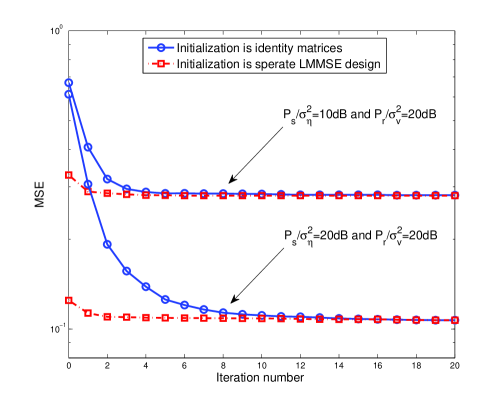
Figure 3: The convergence behavior of the proposed Algorithm 1 when $N_{B}=4$, $N_{R}=4$ and $N_{M,k}=2$ with 2 users.

First, let us focus on the downlink. In downlink, the noise covariance matrices at relay station and mobile terminals are ${\bf{R}}_{{\boldsymbol{\eta}}}=\sigma_{\eta}^{2}{\bf{I}}_{N_{R}}$ and ${\bf{R}}_{{\bf{v}}_{1}}={\bf{R}}_{{\bf{v}}_{2}}=\sigma_{v}^{2}{\bf{I}}_{N_{M}}$, respectively. We define the first hop SNR at the relay station as $P_{s}/{\sigma_{\eta}}^{2}$, and the second hop SNR at mobile terminals as $P_{r}/\sigma_{v}^{2}$. Fig. 3 shows the convergence behavior of the proposed Algorithm 1 for downlink with different second hop SNR at mobile terminals when $N_{B}=4$, $N_{R}=4$, $N_{M,k}=2$. Both initializations with identity matrices and the separate LMMSE design are shown. It can be seen that the proposed algorithm converges quickly, within 20 iterations. Furthermore, the convergence speed with separate LMMSE design as initialization is faster than that with identity matrices. It can also be seen that the two initializations result in the same MSE after convergence.

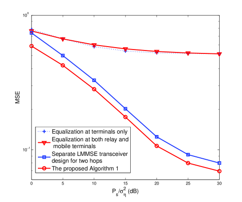
Figure 4: Total MSEs of detected data of the proposed Algorithm 1 and suboptimal algorithms, when $N_{B}=4$, $N_{R}=4$, $N_{M,k}=2$ and $P_{r}/\sigma_{v}^{2}$=20dB.

Fig. 4 compares the total data MSEs of the proposed Algorithm 1 and several suboptimal algorithms versus the first hop SNR $P_{s}/\sigma_{\eta}^{2}$. The second hop SNR at mobile terminals is fixed to be 20dB. The number of antennas is set as $N_{B}=4$, $N_{R}=4$ and $N_{M,k}=2$. The suboptimal algorithms under consideration are

$\bullet$ Direct amplify-and-forward, in which the precoder ${\bf{T}}$ at BS and forwarding matrix ${\bf{W}}$ at relay are proportional to identity matrices. At mobile terminals, LMMSE equalizer for the combined first hop and second hop channel is adopted to recover the signal [3].

$\bullet$ The first hop channel is equalized at relay and then the second hop channel is equalized at mobile terminals, both with LMMSE equalizers.

$\bullet$ Separate LMMSE design proposed for initialization of Algorithm 1.

From Fig. 4, it can be seen that as there is no precoder design at BS for the first two suboptimal algorithms, the data streams at different terminals cannot be efficiently separated by linear equalizers, resulting in poor performances. The separate LMMSE transceiver design has a much better performance. On the other hand, the proposed Algorithm 1 has the best performance among the four algorithms. The gap between the MSEs of the separate LMMSE design and that of Algorithm 1 is the performance gain obtained by additional iterations.

As the proposed Algorithm 1 involves a computational expensive SDP for the precoder ${\bf{T}}$ design, it is of great interest to investigate how much degradation would result from skipping the precoder design. Fig. 5 compares the total data MSEs of the proposed Algorithm 1 and the same algorithm but fixing the precoder ${\bf{T}}\propto{\bf{I}}$. The second hop SNR at mobile terminals $P_{r}/\sigma_{v}^{2}$ is fixed to be 20dB. From Fig. 5, it can be seen that a properly designed precoder significantly improves the system performance when the first hop SNR is high. Without the precoder, the data MSEs exhibit error floors at much lower $P_{s}/\sigma_{\eta}^{2}$. On the other hand, we can also see that increasing the number of antennas at the relay station greatly improves the system performance, as it simultaneously increases the diversity gain of the two hops.

Now, let us turn to the results in the uplink. In uplink case, the noise covariance matrices at relay station and BS are ${\bf{R}}_{{\bf{n}}}=\sigma_{n}^{2}{\bf{I}}_{N_{R}}$ and ${\bf{R}}_{{\boldsymbol{\xi}}}=\sigma_{\xi}^{2}{\bf{I}}_{N_{B}}$, respectively. We define the fist hop SNR at the relay station as $P_{s}/{\sigma_{n}}^{2}$, where $P_{s}=\sum_{k=1}^{K}P_{s,k}$. The second hop SNR at the BS is defined as $P_{r}/\sigma_{\xi}^{2}$.

Fig. 6 shows the convergence behavior of the proposed Algorithm 2 for uplink when $N_{B}=4$, $N_{R}=4$ and $N_{M,k}=2$. Notice that in this case, at each mobile terminal the number of antennas equals to that of the data streams, and Algorithm 2 involves no relaxation. The initialization is identity matrices. It can be seen that Algorithm 2 converges very fast, indicating its superior performance.

Fig. 7 shows the total data MSEs of the proposed Algorithm 2 and suboptimal algorithms, when $N_{B}=4$, $N_{R}=4$, $N_{M,k}=2$ and the SNR at relay station $P_{s}/\sigma_{n}^{2}$ is fixed to be 20dB. The suboptimal algorithms are similar to those for the downlink. In particular, we consider

$\bullet$ Equalization of the equivalent two-hop channel is applied only at the BS.

$\bullet$ Equalization is applied at relay station for the mobile-to-relay channel, and also at BS for the relay-to-BS channel.

$\bullet$ Separate LMMSE design. The first hop is considered as a traditional multiuser MIMO uplink system, and the beamforming matrices are designed using the algorithms in [19] and [21]. The second hop is considered as a point-to-point MIMO system, and the beamforming matrices are designed using the result in [17].

From Fig. 7, it can be seen that the performance of the proposed Algorithm 2 is better than other suboptimal algorithms. However, as the signals from different terminals are cooperatively detected at BS, the gaps between the performance of the suboptimal algorithms from that of Algorithm 2 is much smaller compared to their counterparts in downlink.

When $L_{k}<N_{M,k}$ in the uplink, strictly speaking, Algorithm 2 involves a relaxation, and its performance is not guaranteed. However, a simple variation of Algorithm 1 can be used for beamforming design in this case. Fig. 8 shows the total data MSEs of Algorithm 1 for uplink and Algorithm 2 with rank relaxation, when $L_{k}=2$ and $N_{M,k}=4$. The SNR at BS is fixed at $P_{r}/\sigma_{\xi}^{2}$=20dB. The joint relay forwarding matrix and destination equalizer design in [3] is also shown for comparison. It can be viewed as a design without source precoders at mobile terminals. From Fig. 8, it can be seen that Algorithm 1 and Algorithm 2, which involve the joint design of precoder, forwarding matrix and equalizer perform better than the algorithm in [3]. This indicates the importance of source precoder design in AF relay cellular networks. Furthermore, although Algorithm 2 involves a relaxation, its performance is still satisfactory, and is close to that of Algorithm 1. Finally, it can also be concluded that increasing the number of antennas at relay station can greatly improve the performance of uplink beamforming design for all algorithms.

5 Conclusions

In this paper, LMMSE beamforming design for amplify-and-forward MIMO relay cellular networks has been investigated. Both uplink and downlink cases were considered. In the downlink, precoder at base station, forwarding matrix at relay station and equalizer at mobile terminals were jointly designed by an iterative algorithm. On the other hand, in the uplink case, we demonstrated that in general the beamforming design problem can be solved by an iterative algorithm with the same structure as in the downlink case. Furthermore, for the fully loaded or overloaded uplink systems, a novel beamforming design algorithm was derived and it includes several existing algorithms for conventional point-to-point or multiuser systems as special cases. Finally, simulation results were presented to show the performance advantage of the proposed algorithms over several suboptimal schemes.

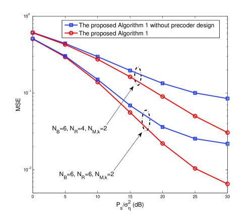
Figure 5: Total MSEs of detected data of the proposed Algorithm 1 with and without precoder design.

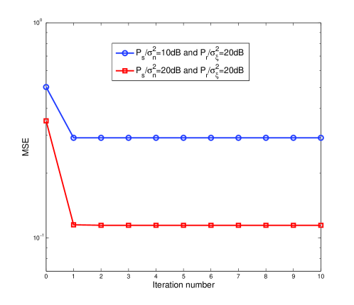
Figure 6: The convergence behavior of Algorithm 2 for uplink when $N_{B}=4$, $N_{R}=4$ and $N_{M,k}=2$.

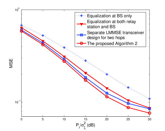
Figure 7: Total MSEs of detected data of Algorithm 2 and suboptimal algorithms, when $N_{B}=4$, $N_{R}=4$, $N_{M,k}=2$ and $P_{s}/\sigma_{n}^{2}$=20dB.

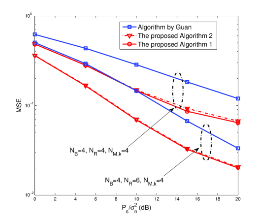
Figure 8: Total MSEs of the detected data of the Algorithm 1, Algorithm 2 with relaxation and the algorithm proposed in [3].

References

• [1] A. Scaglione, D. L. Goeckel, J. N. Laneman, Cooperative communications in mobile Ad Hoc networks, IEEE Signal Process. Magaz. 23 (5) (2006) 18-29.
• [2] J. N. Laneman, D. N. C. Tse, G. W. Wornell, Cooperative diversity in wireless networks: Efficient protocols and outage behavior, IEEE Trans. Inf. Theory 50 (12) (2004) 3062-3080.
• [3] W. Guan, H. Luo, Joint MMSE transceiver design in non-regenerative MIMO relay systems, IEEE Commun. Lett. 12 (7) (2008) 517-519.
• [4] X. Tang, Y. Hua, Optimal design of non-regenerative MIMO wireless relays, IEEE Trans. Wireless Commun. 6 (4) (2007) 1398-1407.
• [5] Y. Rong, X. Tang, Y. Hua, A unified framework for optimizing linear non-regenerative multicarrier MIMO relay communication systems, IEEE Trans. Signal Process. 57 (12) (2009) 4837-4851.
• [6] A. S. Behbahani, R. Merched, A. J. Eltawil, Optimizations of a MIMO relay Network, IEEE Trans. Signal Process. 56 (10) (2008) 5062-5073.
• [7] H. Bolcskei, R. U. Nabar, O. Oyman, A. J. Paulraj, Capacity scaling laws in MIMO relay networks, IEEE Trans. Wireless Commun. 5 (6) (2006) 1433-1443.
• [8] B. Wang, J. Zhang, A. Host-Madsen, On the capacity of MIMO relay channels, IEEE Trans. Inf. Theory 51 (1) (2005) 29-43.
• [9] C.-B. Chae, T. W. Tang, R. W. Health, S.-Y. Cho, MIMO relaying with linear processing for multiuser transmission in fixed relay networks, IEEE Trans. Signal Process. 56 (2) (2008) 727-738.
• [10] R. Zhang, C. C. Chai, Y.-C. Liang, Joint beamforming and power control for multiantenna relay broadcast channel with QoS constraints, IEEE Trans. Signal Process. 57 (2) (2009) 726-737.
• [11] S. Stefania, I. Toufik, M. backer, LTE, the UMTS Long Term Evolution: From Theory to Practice, Wiley, 2009.
• [12] A. Osseiran, etc, The road to IMT-advanced communication systems: state-of-the-art and innovation areas addressed by the WINNER + project - [topics in radio communications], IEEE Communication Magazine 47 (6) (2009) 38-47.
• [13] I. E. Telatar, Capacity of multi-antenna Gaussian channels, European Trans. on Telecommu. 10 (6) (1999) 585-595.
• [14] S. Kay, Fundamental of Statistical Signal Processing: Estimation Theory, Englewood Cliffs, NJ: Prentice-Hall, 1993.
• [15] E. G. Larsson, P. Stoica, Space-Time Block Coding for Wireless Communications, Cambridge University Press, 2003.
• [16] D. Tse, P. Viswanath, Fundamentals of Wireless Communication, Cambridge University Press, 2005.
• [17] H. Sampath, P. Stoica, A. Paulraj, Generalized linear precoder and decoder design for MIMO channels using the weighted MMSE criterion, IEEE Trans. Commun. 49 (12) (2006) 2198-2206.
• [18] J. Zhang, Y. Wu, S. Zhou, J. Wang, Joint linear transmitter and receiver design for the downlink of multiuser MIMO, IEEE Commun. Lett. 9 (11) (2005) 991-993.
• [19] S. Shi, M. Chubert, H. Boche, Rate optimization for multiuser MIMO systems with linear processing, IEEE Trans. Signal Process. 56 (8) (2008) 4020-4030.
• [20] S. Serbetli, A. Yener, Transceiver optimization for multiuser MIMO systems, IEEE Trans. Signal Process. 52 (9) (2004) 214-226.
• [21] M. Codreanu, A. Tolli, M. Juntti, M. Latva-aho, Joint design of Tx-Rx beamforming in MIMO downnlink channel, IEEE Trans. Signal Process. 55 (9) (2007) 4639-4655.
• [22] S. S. Christensen, R. Agarwal, E. de Carvalho, J. M. Cioffi, Weighted sum-rate maximization using weighted MMSE for MIMO-BC beamforming design, IEEE Trans. Wireless Commun. 7 (12) (2008) 4792-4799.
• [23] R. Hunger, M. Joham, W. Utschick, On the MSE-Duality of the broadcast channel and multiple access channel, IEEE Trans. Siganl Process. 57 (2) (2009) 698-713.
• [24] S. Shi, M. Chubert, H. Boche, Downlink MMSE transceiver optimization for multiuser MIMO systems: Dulaity and sum-MSE minmization, IEEE Trans. Signal Process. 55 (11) (2007) 5436-5446.
• [25] A. Beck, Quadratic matrix programming, SIAM Journal on Optimization 17 (4) (2007) 1224-1238.
• [26] S. Boyd, L. Vandenberghe, Convex Optimization, Cambridge University Press, 2004.
• [27] C. Xing, S. Ma, Y.-C. Wu, Robust joint design of linear relay precoder and destination equalizer for dual-hop amplify-and-forward MIMO relay systems, IEEE Trans. Signal Process. 58 (4) (2010) 2273-2283.
• [28] L. Vandenberghe, S. Boyd, Semidefinite programmming, SIAM Review 38(1)(1996) 49-95.
• [29] K.-K. Wong, A. Paulraj, R. D. Murch, Efficient high-performance decoding for overloaded MIMO antenna systems, IEEE Trans. Wireless Commun. 6 (5) (2007) 1833-1843.
• [30] R. de Miguel, V. Gardasevic, R. R. Muller, F. F. Knudsen, On overloaded vector precoding for single-user MIMO channels, IEEE Trans. Wireless Commun. 9 (2) (2010) 745-753.
• [31] C. Xing, Linear Mean-Square-Error Transceiver Design for Amplify-and-Forward Multiple Antenna Relaying Systems, Ph.D. Thesis, The University of Hong Kong, Hong Kong, July 2010.
• [32] R. A. Horn, C. R. Johnson, Matrix Analysis, Cambridge University Press, 1985.
• [33] M. Grant, S. Boyd, Y. Y. Ye, CVX: Matlab Software for Disciplined Convex Programming, available at: http://www.stanford.edu/boyd/cvx, V.1.0RC3, 2007.
Refer to caption