The extinction law for molecular clouds

Abstract

Context. The large optical and near-IR surveys have made it possible to investigate the properties of dark clouds by means of extinction estimates. There is, however, a need for case studies in more detail in order to investigate the basic assumptions when, say, interpreting reddening in terms of column density.

Aims. We determine the extinction curve from the UV to the near-IR for molecular clouds and investigate whether current models can adequately explain this wavelength dependence of the extinction. The aim is also to interpret the extinction in terms of $H_{2}$ column density.

Methods. We applied five different methods including a new method for simultaneously determining the reddening law and the classification of the background stars. Our method is based on multicolour observations and a grid of model atmospheres.

Results. We confirm that the extinction law can be adequately described by a single parameter, $R_{V}$ (the selective to absolute extinction), in accordance with earlier findings. The $R_{V}$ value for B 335 is $R_{V}\,=\,4.8$. The reddening curve can be accurately reproduced by model calculations. By assuming that all the silicon is bound in silicate grains, we can interpret the reddening in terms of column density, $N_{H}\,=\,4.4\ (\pm 0.5)\cdot\,10^{21}\,E_{I-K_{s}}\ cm^{-2}$, corresponding to $N_{H}\,=\,2.3\ (\pm 0.2)\cdot\,10^{21}\cdot A_{V}\ cm^{-2}$, close to that of the diffuse ISM, $(1.8\ -2.2)\cdot 10^{21}\ cm^{-2}$.

We show that the density of the B 335 globule outer shells can be modelled as an evolved Ebert-Bonnor gas sphere with $\rho\,\propto r^{-2}$, and estimate the mass of this globule to $2.5\,M_{\odot}$

1 Introduction

The extinction curve, i.e. the wavelength dependence of the interstellar extinction due to dust particles, has been the subject of numerous investigations in the past fifty years (as exemplified in Table 2). The main driver for these efforts has been the need for restoring the intrinsic spectral properties of the targets, but the extinction curve also carries information on the properties of the dust particles and their origin and development. For a recent review, see Draine (2003). The extinction curve has been defined well for the diffuse ISM (interstellar matter), and even though variations have frequently been reported for different lines of sight, it has been found that these variations can be described by a functional form with only one parameter, $R_{V}\,=\,A_{V}/E_{B-V}$ as shown by Cardelli et al. (1989) (hereafter CCM), who also found that the extinction in a few lines of sight through the outskirts of dark clouds can be defined in the same way. However, as the purpose of their investigation was to include the strongly variable 217.5 nm bump, the list of background stars is restricted to O and early B stars for which the emission from the surrounding HII and PDR regions may - as noted by the authors - add uncertainty to the deduced extinction curve. This is a particular problem in the infrared where a contribution of free-free nebular emission may artificially increase the derived $R_{V}$ value. Using a large sample (154) of obscured OB stars, He et al. (1995), concluded that even though the $R_{V}$ value may vary between 2.6 and 4.6, the near-IR ($\lambda\,>0.9\mu$m) extinction curve can be well-fitted to a power law with an exponent $-$1.73$\pm$0.04. The variation in $R_{V}$ value indicates that the light paths may partly pass through dark clouds, but this aspect is hard to quantify. In an investigation of the Taurus cloud complex, Whittet et al. (2001) observed 27 background, early type stars from the U to the K band, and most of these stars (23) have only moderate extinction ($A_{V}\,<\,3.4$) and the corresponding $R_{V}$ values average around 3.0, i.e. typical of the diffuse ISM. The remaining four stars, with $A_{V}$ values in the range 3.6–5.7, have higher $R_{V}$ values, indicating that these light paths probe denser regions with larger particles.

In our view, there is a need for further studies of the extinction curve in deeper parts of dark clouds and it is important, as far as possible, to include the UV/blue region since grain growth will first affect the extinction curve at shorter wavelengths. Thus, even though a ”universal” power law may describe the shape of the extinction curve well in the near-IR, the particle size distribution, and thus the column density of dust mass, may be poorly determined. The 2Mass all-sky survey (Skrutskie et al. (2006)) has proven extremely useful in providing extinction maps of dark cloud complexes, and it is important to find out how well the conversion factor $N_{H_{2}}/E_{J-K_{s}}$ can be determined. This is the main scope of the present investigation. We focus on the well known dark globule B 335, and based on multi-colour observations, we apply different ways to determine the extinction and, in particular, a new method that allows us to both classify the background stars and determine the extinction. For comparison, we also include observations of an early type star behind the Cha I cloud.

2 Observations and data reductions

B335 (RA(2000) = 294.25, DEC(2000)  = 7.57) and a reference field (RA(2000) = 293.54, DEC(2000) = 7.62), were observed using the NTT at La Silla during four nights 2006-06-27–29. The reference field, hereafter called the free field (B335ff in the table) was selected to be at the same galactic latitude as B335 and free from cloud extinction. The observations are summarized in Table 1.

Table 1: Observation log.

object	camera	filter	centre	exp time	exp time
			$\lambda$	ea image	total
			[nm]	[s]	[s]
B335	EMMI-blue	U602	354.0	720	24000
B335	EMMI-red	Bb605	413.2	720	8500
B335	EMMI-red	g772	508.9	500	4000
B335	EMMI-red	r773	673.3	300	2000
B335	EMMI-red	I610	798.5	200	1000
B335	EMMI-red	spec	grism4		6000
B335	NOTCAM	Ks	2144.	900	1000
B335ff	EMMI-blue	U602	354.0	720	4000
B335ff	EMMI-red	Bb605	413.2	720	3000
B335ff	EMMI-red	g772	508.9	500	2000
B335ff	EMMI-red	r773	673.3	300	1000
B335ff	EMMI-red	I610	798.5	200	500
Cha035	EMMI-blue	U602	354.0	720	7100
Cha035	EMMI-red	Bb605	413.2	720	720
Cha035	EMMI-red	g772	508.9	480	480
Cha035	EMMI-red	r773	673.3	300	300
Cha035	EMMI-red	I610	798.5	300	300

All object frames have been preceded and followed by exposures of the standard star SA111-1195 (Landolt (1992)) in respective filter. The basic reductions (bias subtraction, dark correction, flat-fielding, cosmic ray reduction) were carried out using standard $IRAF$ routines. Then the $IRAF$ astrometric programs are used for registering and co-adding the images using $Skyview$ facilities for astrometric data on stars common to all images of an object. The individual frames were noise weighted by the inverse of the errors of the stars in the middle magnitude range. The star finding program $sextractor$ has then been used to tabulate stars and positions. Photometry of the co-added images was then carried out using the $DAOPHOT$ photometry package.

The Landolt equatorial standard star SA111-1925 was classified with the help of the SED simplified method (see below) to be an A3V star. Using stellar models and the filter characteristics the colour correction from Landolt (1992) filters (including the detector spectral response and the atmospheric transmission) to the Eso NTT-EMMI Gunn and Bessel filter sets could be made.

These data have been combined with data from the Two Micron All Sky Survey (2MASS) Point Source Catalog(PSC) (Skrutskie et al. (2006)) thus extending the stellar data with the $J-H-K_{s}$ measurements (where these exist) in the B335 and the free field B335ff.

The EMMI-images and the 2Mass data have been complemented by an image taken with the NOTCAM at the Nordic Telescope on La Palma using the $K_{s}$-filter (by M Gålfalk, 2005-06-30. (The image reduction is described in Gålfalk & Olofsson (2007)). The photometric calibration was based on the 2Mass field stars with low photometric errors.

Finally $IRAC$ data from the Spitzer data archive have been used. The Spitzer archived images were analyzed with the Mopex-software package (Makovoz & Khan (2005), Makovoz & Marleau (2005), Masci et al. (2004)) to give the stellar magnitudes.

All the stellar data have finally been compiled in tables for B335 and the free field containing object positions, magnitudes and magnitude errors in all the relevant filters.

3 Results

3.1 The pair method

There are a few stars in the B 335 region for which we have spectroscopy. Some of these have been classified as K7III stars. They are obscured to varying degrees. One of them, No. 2, is more heavily obscured. By comparing these stars, and normalizing to $E_{I-K_{s}}$, we directly get the extinction curve (apart from the extrapolation to zero wave-number i.e. $A_{K_{s}}/E_{I-K_{s}}$). Unfortunately, the faintness of the obscured star in the U band results in a large uncertainty regarding the the derived extinction in the UV.

3.2 Statistical reddening

Lacking any information on the intrinsic SED:s (spectral energy distributions) of the stars, the traditional method is to determine the reddening vector for the various colour index combinations. The main problem in this approach is the wide spread of the intrinsic colours of the stars, as is shown in Fig 1. For this reason it is useless for estimating the extinction towards individual anonymous stars. However, it is a robust and simple method and worth looking closer at. In Fig 2 we show the distribution of the colour indices $B-K_{s}$ versus $U-K_{s}$ for the two fields. The expected intrinsic scatter is clearly seen in the free field, but it is also clear that the contours for the B 335 field are both stretched and shifted due to the reddening. The slope of the line, $E_{B-K_{s}}/E_{U-K_{s}}$, is well defined.

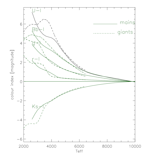
Figure 1: The colours as derived from the stellar atmospheric models from Hauschildt et al. (1999)

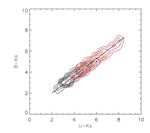
Figure 2: The contours represents the number density of colour indices for the stars in the B 335 field and the reference field (black). The fitted line represents the direction of the reddening vector.

Figure 3: The median of the logarithmic projected separation (of the seven nearest) stars vs the U-magnitude limits. The dashed curves shows one standard deviation for the object in the B335circle.

3.3 Star counting

Star counting is a straightforward way of estimating the interstellar extinction. The star count method goes back to Wolf23 and is based on the projected surface density of stars in an obscured area compared to that of a region without (foreground) extinction. The stars in magnitude intervals are counted in each cell of a grid of cells. Later the method was improved to instead count the number of stars up to a magnitude level. In this way the chosen grid cell size is a compromise between spatial and statistical resolution. Cambrésy (1999) presented an improved method where the statistical resolution is fixed by measuring the local star density expressed as the projected distance to the stars in the local surrounding. In the free field a relation of the mid (mean or median) distance $d_{free}$ of the neighbouring stars up to a magnitude limit $m_{limit}$ gives a linear relationship as shown in Fig 3.

$$log(d_{free})=C_{linear}\cdot m_{limit}$$ (1)

where $C_{linear}$ is a constant. This relation is linear in a range determined by the completeness level of magnitudes. For the reference as well as for the object field we have the relation $m_{limit}\ =\ m_{0}\ -\ (1./C_{linear})\cdot log(d)$ see Fig 3, differing by different values for the constant $m_{0}$ in the reference and the object field, namely the difference in the extinction between the two fields.

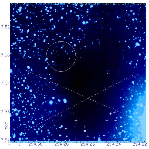
Figure 4: B335 in the U-filter with the circle shown in which extinction estimation by star counting has been performed in Fig 3. The dashed lines mark the cloud centre and outflow cones, + signs mark the stars that contribute in Fig 13 to the estimation of the cloud radius.

The star count method is simple and straightforward. If the reference field is representative for the star field behind the cloud, the measurement gives the extinction of the foreground cloud. In contrast to methods based on the colour of the stars, star counting gives the total extinction, and the otherwise required extrapolation from the longest wavelength to infinity is avoided. However, in practice the assumption on a smooth distribution of background stars is not valid and this limits the accuracy. In addition, it gives a poor spatial resolution compared to methods based on reddening of the background stars. Still, for comparison, we have applied the method of Cambrésy (1999) and we have selected a sub-region in the B 335 field, see Fig 4. The result is shown in table 3.

3.4 The SED method

Several multicolour systems (e. g. the Strömgren four-colour Strömgren (1966), or the Vilnius seven-colour photometric system Straižys (1993)) have been extensively used to classify stars and quantify stellar properties. They are based on measurements in well defined narrow-band filter sets and the correction for the interstellar extinction is carried out by adopting an extinction law.

We propose a more general way to determine the intrinsic qualities of stars as well as the extinction curve, based on multicolour measurements. For a given star, the observed SED represents the combination of the intrinsic SED of the star, the distance and the extinction along its light path. Without any separate knowledge of the star and without any assumption of the wavelength dependence of the extinction, there is no way to determine the intrinsic SED of one star and the extinction. However, if we consider two (or more) adjacent stars and assume that their cloud extinction is the same, then it is possible to find both the spectral class of the stars and the extinction of the intervening part of the cloud (see Appendix A).

There are practical limitations also for this method. One is the assumption of equal extinction for adjacent stars, which is risky in regions of strong gradients. Another is the tendency for the reddening vector in a colour index diagram to be parallel to the locus of the intrinsic colours of the stars as seen in Fig 2. In other words, it may be difficult to tell whether a star is red because it is intrinsically red or reddened by the extinction. The degeneracy was resolved by choosing several combinations of neighbouring stars and noting the consistency in the $T_{eff}$ determination. It turns out that a broad spectral coverage is essential and that it is indeed possible to find trustworthy solutions. To represent the intrinsic SED:s of the stars we have used model atmospheres kindly provided by P. Hauschildt, which cover the temperature range 2600 K to 10000 K at two surface gravities ¹⁰log g equal to 0 and 4.5 representing the main sequence stars and the giant stars respectively. In order to keep the number of model SED:s at a manageable level, we only include one metalicity (solar). The synthetic spectra cover the spectral range $0.01\mu\,<\lambda\,<\,100\,\mu$ at a high spectral resolution. These model atmospheres are described by Hauschildt et al. (1999). The sensitivity function (including filter transmission, detector sensitivity and atmospheric transmission) was used to calculate the synthetic colours.

Figure 5: Extinction vs wavenumber $[1/\mu m]$ for several stars in the differently dense regions of the B335 cloud. The dashed curves are the $R_{V}$ fitted CCM curves. The curve marked Cha035 is a corresponding measurement of the extinction toward a star behind the Chamaeleon I cloud.

Fig 5 shows the extinction in the whole wavelength range from 0.35 to 8. $\mu m$ for some stars in the cloud border high-density area of B335. For each of these we fit a CCM curve. We first note that CCM curves well describe the observed extinction curves and that the $R_{V}$ values are in the range $R_{V}$ = 3.4–5.5 with an average of $R_{V}$ = 4.8. A similar extinction curve constructed from the measurements in the Cha I cloud (marked Cha035) is also drawn in the same diagram (together with its fitted CCM curve).

Figure 6: Extinction vs wavenumber $[1/\mu m]$ as the median for several stars (whose sight line extinctions are shown in 5). The CCM curve (dashed line) fitted to that extinction has a $R_{V}$ of 4.8. The grain distribution model shown in Fig 11 gives a good fit to the observations (dotted line). The scattering part, labelled ”scattering” shows the scattering part of the extinction.

The normalized and averaged extinction from B335 is in Fig 6 compared with a CCM curve with $R_{V}$ = 4.8.

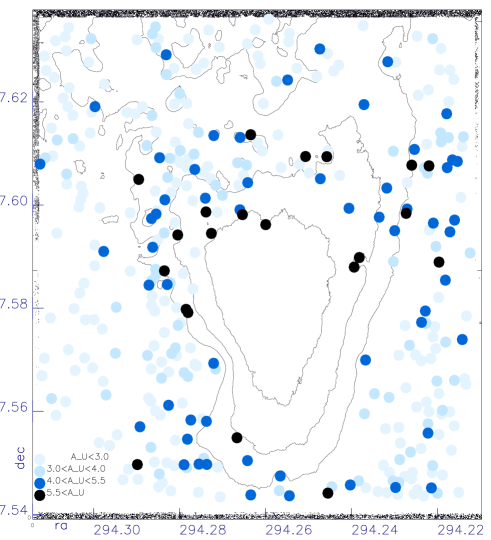
Figure 7: Extinction as calculated with the simplified SED method for each star (only stars with U and 2Mass Ks measurements are included). The contours mark the background flux in the U band due to the scattered interstellar radiation field. The step between contour lines is $\sim 5\cdot 10^{-2}\,\mu Jy\,arcsec^{-2}$.

3.5 A simplified SED method

All the methods tested above confirm that the extinction in the optical and NIR wavelength range can accurately be described by the CCM curve. This means that we can simplify the SED method by just leaving the $R_{V}$ value and a colour excess (e.g. $E_{I-K_{s}}$) as parameters and search for the best combination of R, E and model SED. This can conveniently be done for each star resulting in an extinction map with high resolution, as in Fig 7. In this figure we compare the surface brightness due to the scattered interstellar radiation field to the extinction of the individual field stars. As expected, the stars with the highest extinction are closest to the dark core of the globule. In this figure we have included faint stars with relatively poor photometry. Our optimization scheme allows the $R_{V}$ value to vary between 2 and 12 and, surprisingly, we notice a large variation. For faint stars with poor photometry as well as for stars with little extinction, this can be explained as spurious, but how about the lines of sight toward more obscured stars with accurate photometry - can we trust the deduced R_V values? If we restrict the sample to stars with $E(U-K_{s})>3$, $\sigma K_{s}<0.3$ we get the $R_{V}$ distribution shown in Fig 8. This sample includes late stars for which the model atmospheres probably are less reliable and for which we expect larger departures from solar metallicity. This means that the free parameter R_V could to some extent compensate for such non-perfect matching of the model colours to the true intrinsic colours. If we restrict the sample further by only including stars with T${}_{eff}>7500$ K, for which we assume that the uncertainties are less we still find a scatter, but interestingly also a trend; the R_V value correlates to the extinction, see Fig 9.

We have applied the five methods in determining the extinction curve towards B 335 and in table 3 we summarize the results. The different methods agree well.

Table 2: Extinction descriptions

reference	wavelength	description
	range $[\mu m]$	$R_{V}\,=\,A_{V}/E_{B-V}$
Bailey & Williams (1988)	$0.9\ \ <\ \lambda\ >\ 3.5$	$A_{\lambda}/A_{V}\ \varpropto\lambda^{-\alpha}$
Cardelli et al. (1989)	$0.35\ <\ \lambda\ <\ 0.9$	$A_{\lambda}/A_{V}\ =\ f_{A}(1/\lambda,\ 7)+f_{B}(1/\lambda,\ 7)/R_{V}$
	$0.9\ \ <\ \lambda\ <\ 3.5$	$A_{\lambda}/A_{V}\ =\ C0\cdot(1/\lambda)^{\alpha}+C1\cdot(1/\lambda)^{\alpha}/R_{V}$
Fitzpatrick & Massa (1990)	$0.11\ <\ \lambda\ <\ 0.3$	5-parameter model
Fitzpatrick (1999)	$\lambda\ >\ 0.11$	$R_{V}\ tabled\ A_{\lambda}/A_{V}$
Indebetouw et al. (2005)	$1.25\ <\ \lambda\ <\ 5.$	$log(A_{\lambda}/A_{V})\ =\ f_{A}(log(\lambda),\ 2)$

Table 3: Comparison of normalized extinctions.

			EMMI						2Mass			Spitzer
band			U602	Bb605	g772	V606	r773	I610	J	H	$K_{s}$	$[3.6\mu]$	$[5.8\mu]$
$\lambda\ \ \ [nm]$			354.0	413.2	508.9	542.1	673.3	798.1	1258.5	1649.7	2157.2
$\Delta\lambda\ [nm]$			53.7	109.4	75.3	104.8	81.1	155.2	300.	300.	300.	800.	1500.
source	medium	RV	E($[\lambda]$- Ks)/E(I - Ks)
this work
B335 SED-method	B335	4.8	2.29	2.02	1.72		1.25	1.00	0.33	0.11	0.00	-0.15	-0.22
B335 SED-stdv			0.06	0.04	0.01		0.01		0.03	0.02		0.05	0.06
B335 pair-method			2.39	2.11	1.87		1.23	1.00	0.28	0.15	0.00	-0.06	-0.15
B335 pair-stdv			0.08	0.08	0.11		0.07		0.03	0.01		0.01	0.03
B335 statistical			2.32	1.96	1.66		1.16	1.00	0.34	0.09	0.00
B335 stat-stdv			0.15	0.10	0.05		0.04		0.04	0.04
B335 star count			1.9	1.7	1.5		1.3	1.00	0.00
B335 star-stdv			0.4	0.5	0.5		0.4		0.2
	medium	RV	E($[\lambda]$- Ks)/E(I - Ks)
Cardelli et al. (1989)		4.8	2.30	2.14	1.76	1.65	1.31	1.00	0.35	0.14	0.00	-0.14	-0.20
Rieke & Lebofsky (1985)	dISM	3.09	3.84	3.28		2.40	1.72	1.00	0.46	0.17	0.00
Martin & Whittet (1990)	dISM	3.0	3.91	3.22		2.37	1.70	1.00	0.44	0.16	0.00
He et al. (1995)	dISM	3.08	3.21	2.67		1.96	1.52	1.00	0.36	0.13	0.00
Fitzpatrick (1999)	dISM	3.1	3.71	3.09		2.26	1.62	1.00	0.41	0.14	0.00
dISM stands for diffuse ISM

Figure 8: The $R_{V}$ distribution of the extinction towards the background stars with good photometry and with $E(I-K_{s})>3$. The median $R_{V}$value is $\sim 4.8$.

Figure 9: The $R_{V}$ for selected early type stars as a function of the excess $E_{U-K_{s}}$ showing a tendency for higher $R_{V}$ values at higher excesses.

Figure 10: This figure, based on the same sub-sample as Fig 8, shows the statistical spatial correlation of the $R_{V}$ values. There is no significant tendency for adjacent stars to have similar $R_{V}$ values.

4 Interpretation

4.1 The extinction curve – local variations?

Our results show that CCM curves well represent the extinction in the test cloud, B 335 as well as for one location in the Cha I cloud. The simplified SED method resulted in a distribution of R_V values (Fig 8), and one may wonder whether there is any local variations, apart from the tendency of a correlation between $R_{V}$ value and extinction 9. In Fig 10 we show that there is no tendency for such local variation, and we conclude that the scatter shown in Fig 8 is probably due to non-perfect matching of the model colours to the real ones as well as the observational uncertainties.

Figure 11: The grain size distribution for the average extinction as shown in Fig 5 (full drawn line: graphite, dashed: silicates). As a comparison the WD2001 $R_{V}\,=\,3.1$ grain distribution dotted and dash-dotted. The model parameters used are shown in Tab 4. ($dN_{grain}/da$ grain size distribution; a grain particle radius; $N_{H}$ H-column density.)

4.2 Grain size distribution

We apply the grain size distribution model constructed by Weingartner & Draine (2001) (hereafter WD2001) and using Mie calculations (cf. Bohren & Huffman (1983)) we optimise the relative abundance of the different components to fit the observed extinction curve. The model fit to the observed extinction is very good as shown in Fig. 6. In Fig. 11 we compare the resulting size distributions of the graphite and the silicate grains to that for the diffuse ISM, and as expected the grains are larger in the molecular cloud. Even though this general tendency for larger grains in the globule is a robust and expected result, we cannot push the interpretation much further as the model fit to the observed extinction includes many parameters, some of these not well constrained by the observations.

Table 4: Grain distribution parameters according to WD2001

	WD2001 grain model parameters
parameters	$b_{C}$	$C_{g}$	$C_{s}$	$\alpha_{g}$	$\alpha_{s}$	$\beta_{g}$	$\beta_{s}$	$a_{t,g}$	$a_{t.s}$
B335 (mean of several sightlines)	1.3	$3.55\cdot 10^{-11}$	$7.33\cdot 10^{-14}$	-1.4	-1.5	-0.240	-3.02	$3.88\cdot 10^{-3}$	0.271
WD2001 table 1 $R_{V}\,=\,3.1$	4.0	$2.9\cdot 10^{-11}$	$1.3\cdot 10^{-13}$	-1.8	-2.1	-0.132	-0.114	8.98	0.169

Figure 12: The total particle masses for the grain size distribution shown in Fig. 11 as a function of the U-extinction. The slope of the curve corresponds to $23\,(\pm 3)\,\mu g\,cm^{-2}\ magnitude^{-1}$.

4.3 The column density

In view of the possible spatial variations of the grain properties we combine neighbouring stars in pairs, under the assumptions

• that the extinctions are represented by CCM functions

• that they have similar grain size distribution and

• that the extinction differences depend on a scale factor only.

Even though our model fits show variations in the carbon/silicate ratio, the total amount of dust mass relates closely to the extinction, and we find the following relation (Fig 12):

grain mass = $23\,(\pm 2)\cdot A_{U}\,\mu g\,cm^{-2}$.

We now turn to the average extinction curve (SED method) in table 3. Assuming that all silicon is bound in these grains as silicates and a ’Cosmic’ abundance of $[Si]\,=3.63\cdot 10^{-5}\cdot[H]$ (Savage & Sembach (1996)) we find the following relation:

$N_{H}\,=\,4.4\,(\pm\,0.5)\,\cdot 10^{21}\cdot E_{I-K_{s}}\,cm^{-2}$

If we trust the model extrapolation to zero wave-number and interpolate between the g- and r-filters we get the relation:

$N_{H}\,=\,2.3\,(\pm\,0.2)\,\cdot 10^{21}\cdot A_{V}\,cm^{-2}$

for B335, which should be compared to the relations found in the literature (e g Bohlin et al. (1978), Predehl & Schmitt (1995), Ryter (1996), Vuong et al. (2003)) from UV Lyman $\alpha$ and X-ray analyses
$N_{H}\,=\,1.8-2.2\cdot 10^{21}\cdot A_{V}\,cm^{-2}$,

Figure 13: The B extinction vs radius [arcsec] from the centre at the protostar in the southern sector of the cloud (Fig 4). The curve marks the projected density for a gas sphere with $\rho\,\propto\,r^{-2}$ with an effective radius 190 [arcsec].

4.4 The mass of B 335

The young source in the middle of the globule has an East–West bipolar outflow with an opening angle of $25^{\circ}\,\pm 5$ (Cabrit et al. (1988) and Hirano et al. (1992)). However, the pre-stellar density profile in regions away from the outflow (see Fig 4) has probably been roughly conserved. We consider a sector in the south direction and plot the extinction as a function of projected radius in Fig 13.

We can trace the extinction for $A_{B}<10$, which means outside a region at radii $>1^{\prime}$ from the cloud centre, corresponding to a distance of 0.03 pc. One of several models of the globule, that has been discussed (Larson (1969), Penston (1969), Shu (1977)), is the gas sphere evolved from the isothermal gravitationally compressed gas sphere with an undisturbed outer shell and and a collapsing centre. In the undisturbed shell the density varies as $\rho(r)\,=\,\kappa/r^{2}$ as described by Shu (1977). The projected density can be fitted to the the extinction profile deduced from sight-lines to the stars marked in the Fig 4 and shown in Fig 13. The effective cloud radius of the globule thus estimated is of the order of $R_{cloud}\,\simeq\,190\,arcsec\,(\bigtriangleup R_{cloud}\,\pm\,\sim 20\,arcsec$).

Thus assuming a gas sphere model with $\rho(r)\,\propto\,r^{-2}$ in line with the findings by Harvey and coworkers (Harvey et al. (2001), Harvey et al. (2003a), Harvey et al. (2003b)) we can estimate the mass $M_{B335}$ of the globule.
Given the cloud radius, the density gradient and the sound speed $a=\sqrt{k\cdot T/\mu}$ we get

$$M_{B335}\,=\,\frac{2\cdot a^{2}\cdot R_{cloud}}{G}\\$$ (2)

where G is the gravitation constant. From molecular line data Zhou et al. (1990) estimated the effective speed of sound $a$ to be $230\,m/s$ , which corresponds to a kinetic temperature of $13^{o}K$. With the cloud model and the sound speed the mass $M_{B335}$ can thus be estimated to be $2.2\,\pm\,0.2\,M_{\odot}$ (apart from the error in the estimate of the distance to the globule).

The more direct way for handling this gas sphere-model is to use the estimation of the measured silicate grain column density $\delta_{silicates}$ transformed into H-mass column density $\delta_{H}$ to get the globule mass $M$. The protostar is assumed to be located in the centre of the cloud. Thus with the impact radius b for a number of sightlines and their H-mass column densities the simple calculations described in Appendix B allow the globule mass to be estimated.

With the globule radius of $190\,\pm\,\sim 20\,arcsec$ the globule mass for sightlines outside of the outflow cone is found to be $2.5\,\pm 0.2\,M_{\odot}$. The three sight lines through or near the outflow cone of the YSO in B335 (marked #10, 84, 112 in the Fig 14) result in lower mass estimates, that average to $2.0\,\pm 0.1\,M_{\odot}$. These total globular-mass estimates are in agreement with the estimation of $2.2\,M_{\bigodot}$ done by Harvey et al. (2001), when corrected for the distance estimate (Olofsson & Olofsson (2009). That leaves a mass of less than 1.0 solar mass within 1 arcmin (the closest sight line in this study) from the centre star.

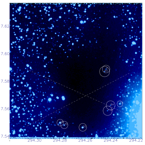
Figure 14: The map marks the sightlines for which the extinction measurements have been done in Fig 5 and for which the globule mass has been estimated. The dashed lines mark the cloud centre and outflow cones.

Figure 15: The difference between the extinctions from the different methods (from Tab 3) and the SED-method with the standard deviations marked in the individual estimates as error bars.

5 Discussion

As a next step it would be natural to investigate a number of molecular clouds and the question is which method should be used. We have used five different methods to determine the extinction curve in a molecular cloud. Within the uncertainties, all methods give the same result (see Tab 3 and Fig 15). There are advantages and disadvantages connected to the different methods depending on the aim of the investigation.

The pair method requires spectroscopic observations in addition to the multi-colour observations. As the stars tend to be very faint in the optical region, the spectroscopy should be carried out in the infrared. The requirement of finding pairs with identical spectral classes that in addition have significantly different extinction, means in practice that quite an extensive spectrometry program should be planned for. On the other hand, given the spectral class, the intrinsic SED is known and the reddening curve can be determined to each star. This is the method we used for the Cha  I 35 included as a comparison in Fig 5. One potential problem is of course that the line of sight may include some background extinction from the diffuse ISM.

The statistical reddening method is simple and robust but it suffers from the problem of separating the large intrinsic scatter of the colour indices from the effect of reddening. It can obviously not be used to gain information on the extinction to individual stars, but it serves well as a complement to more detailed methods.

The star count method is not well suited for determining the extinction curve. It has several shortcomings and the only advantage, that it in principle determines the absolute extinction is not very useful as the accuracy is too poor.

The SED method allows the determination of the extinction in many sub-regions of the cloud and, like the previous methods, it does not include any assumption on the functional shape of the extinction. It is , however, computationally slow.

The simplified SED method is based on our finding that the extinction actually can be characterized by a CCM curve. This may not necessarily be true in all clouds, but it should suffice to first use e.g. the statistical reddening method to check whether a CCM curve can be applied.

If so, the simplified SED method has the advantage of defining the extinction curve towards each star. It must of course be realized that e.g. non-resolved double stars, having flatter SED:s than single stars, would cause spurious $R_{V}$ determinations. This is probably part of the scatter seen in Fig 8. Actually, it could for this reason be justified to exclude stars with extreme $R_{V}$ values in constructing the extinction map of the cloud.

We have determined the extinction curve in the form $E_{[\lambda]-K_{s}}/E_{I-K_{s}}$, and our model fit allows us to estimate the corresponding column density. We have used $E_{I\,-\,K_{s}}$ as the reference colour excess, but in practice there is a number of different I band filters being used and for this reason, and also because of the all-sky coverage of the 2Mass survey it may be more useful to relate to $E_{J-K_{s}}$, even though the error bars are slightly larger. The H-column density results are summarized in Tab 5 and compared with some often cited literature values.

Table 5: H-column density comparison.

source	medium	method	ratioes $N_{H}/A\cdot 10^{-21}\ cm^{-2}$
			$N_{H}/E_{B-V}$	$N_{H}/A_{V}$	$N_{H}/E_{I-K_{s}}$	$N_{H}/E_{J-K_{s}}$	$N_{H}/E_{H-K_{s}}$	$N_{H}/A_{J}$
this work	B335	multicolour		$2.3\,(\pm 0.2)$	$4.4\,(\pm 0.5)$	$15.3\,(\pm 1.9)$	$47\,(\pm 8)$	$7.5\,(\pm 0.8)$
Bohlin et al, 1978	diffuse ISM	Lyman $\alpha$	5.8	1.87
Bohlin et al, 1978	$\rho$ Oph	Lyman $\alpha$	15.8
Predehl et Schmitt, 1995	diffuse ISM	X-ray	5.3	$1.79\,\pm 0.03$
Ryter, 1996	diffuse ISM	Lyman $\alpha$ and X-ray	6.8
Vuong et al, 2003	$\rho$ Oph	X-ray						$5.6\,(\pm 0.4)$
Winston et al. (2007)	Serpens	X-ray					11.5

One problem in going from the observed reddening curve (which relates to a colour index) to the true extinction curve (which relates to a certain wavelength) is the extrapolation to zero wave-number. Both the CCM curve and our dust model fittings provide this extrapolation, but it would still be desirable to include measurements at longer wavelengths. This will be presented in a forthcoming paper (Olofsson & Olofsson, in preparation), where we also will include ices in the measurements and the modelling.

6 Conclusions

• The extinction in the B 335 globule follows a CCM curve with $4.<R_{V}<6.$.

• A dust-to-extinction relation has been established: grain mass = 23. A${}_{U}\,\mu$g cm^-2.

• The relation between reddening and hydrogen column density is $N_{H}\,=\,4.4\cdot\,10^{21}\,E_{I-K_{s}}\,cm^{-2}$

• Assuming a gas sphere with the outer shell modelled with a density profile as $\rho(r)\,\propto\,r^{-2}$, we find an effective globule radius of 190 arcsec. The mass of the B 335 globule is estimated to be $M_{B335}\,=\,2.5\,M_{\bigodot}$

Appendix A SED method

The analysis is based on models for stellar atmospheres and for the interstellar medium extinction. The idea is that combining several star in a group with neighbouring sightlines there is a part of the extinction common to all in the group. This allows us to create an equation system containing the colour indices $CI([\lambda_{i}]-[\lambda_{0}])$ from multi-filter measurements of each star in the group. For a group of three we have for filter $[\lambda_{i}]$ and star#1, 2 and 3

$$CI([\lambda_{i}]\ -\ [\lambda_{0}])_{1} = CI([\lambda_{i}]\ -\ [\lambda_{0}])_{0,1}+A_{\lambda_{i}}\ -\ A_{\lambda_{0}}$$

$$CI([\lambda_{i}]\ -\ [\lambda_{0}])_{2} = CI([\lambda_{i}]\ -\ [\lambda_{0}])_{0,2}+A_{\lambda_{i}}\ -\ A_{\lambda_{0}}+\Delta E_{2}$$

$$CI([\lambda_{i}]\ -\ [\lambda_{0}])_{3} = CI([\lambda_{i}]\ -\ [\lambda_{0}])_{0,3}+A_{\lambda_{i}}\ -\ A_{\lambda_{0}}+\Delta E_{3}$$

where $CI([\lambda_{i}]-[\lambda_{0}])_{\ast}$ are the measured inputs, while the $CI([\lambda_{i}]-[\lambda_{0}])_{0,\ast}$ are the parameterized stellar models for the intrinsic colours with parameters like effective temperature $T_{eff}$, surface gravity and metallicity. Finally $A_{\lambda_{i}}\ -\ A_{\lambda_{0}}$ is the common excesses, namely that of star#1. The other stars may have the additional excesses $\Delta E_{\ast}$, caused by the ISM-extinction between the background stars. As this also can be parameterized to follow e g a CCM-function we have a non-linear over-determined equation system, that can be solved by an optimizing technique for $A_{\lambda_{i}}\ -\ A_{\lambda_{0}}$ and the stellar model parameters of the stars.

In the application described the stellar models have been restricted to those with solar metallicity and two surface gravities, one for the main sequence stars and one for giants.

Thus the number of parameters to be solved are

• $T_{eff}$ one effective temperature for each star.

• $A_{\lambda_{i}}\,-\,A_{\lambda_{0}}$ one excess parameter for each filter measurement.

• $\Delta E_{\lambda}$ : The interstellar extinction CCM-characterization parameter $R_{V}$ for the determination of the $\Delta E_{\lambda}$’s. There is a proportionality constant attached to each $\Delta E_{\lambda}$, as well, to determine all its $\lambda$’s.

So, for three stars and eight filters the number of parameters are 3(Teff’s) + 7(colour indices) + 1(CCM $R_{V}$) + 2(proportionality constants) equals 13 parameters (to be fitted to 21 measured colour indices).

Appendix B Mass determination from column densities.

With an assumed model for the globule mass distribution and measurements of column densities it is possible with simple calculations to get estimates of the globule mass. In this case we assume that our column density measurements are made in the still undisturbed shell of the globule, whose centre is known as well as the impact radius b for the column density measurement. Then with the following variables:

$$\begin{array}[]{lp{0.8\linewidth}}R_{cloud}&cloud radius\\ \emph{b}&impact radius from cloud centre\\ m&calculated globule mass\\ mol_{silicate}&molecular weight of silicates = 172\\ mol_{H}&molecular weight of H\,+\,He=\,1.25\\ $[Si]$&abundance of Si\ \ $[Si]\ =\ 3.63\cdot 10^{-5}\ \cdot\ [H]$\\ \rho(r)&density at radius r\\ \delta_{silicate}(b)&measured column density of silicates at b\\ \delta_{H}(b)&from $\delta_{silicate}$ calculated H-column density at b\\ \end{array}$$

The mass can be calculated in the following way:

$$\rho(r) = \kappa\ /\ r^{2}$$

$$\delta_{silicate}(b) = (2\ \kappa\ /\ b\ )\cdot\ \arccos(b\ /\ R_{cloud})$$

$$\delta_{H}(b) = \delta_{silicate}(b)\ \cdot mol_{H}/\ ([Si]\ \cdot\ mol_{silicate})$$

$$\kappa = \delta_{H}(b)\cdot b/(2\cdot\ \arccos(b\ /\ R_{cloud}))$$

$$m = 4\pi\ \int_{0}^{Rcloud}\rho\ \cdot\ r^{2}\ \cdot\ dr$$

$$m = 4\pi\ \int_{0}^{Rcloud}(\kappa/r^{2})\ \cdot\ r^{2}\ \cdot\ dr=4\pi\ \cdot\ \kappa\ \cdot\ R_{cloud}$$

$$m = 2\pi\cdot\delta_{H}(b)\cdot b\cdot R_{cloud}/\arccos(b\ /\ R_{cloud})$$

If more than one column density measurement at different impact radii b are available the parameter $R_{cloud}$ can be determined as well as the globule mass.

References

- Bailey & Williams (1988) Bailey, M. E. & Williams, D. A., eds. 1988, Dust in the universe; Proceedings of the Conference, Victoria University of Manchester, England, Dec. 14-18, 1987
- Bohlin et al. (1978) Bohlin, R. C., Savage, B. D., & Drake, J. F. 1978, ApJ, 224, 132
- Bohren & Huffman (1983) Bohren, C. F. & Huffman, D. R. 1983, Absorption and scattering of light by small particles, ed. D. R. Bohren, C. F. & Huffman
- Cabrit et al. (1988) Cabrit, S., Goldsmith, P. F., & Snell, R. L. 1988, ApJ, 334, 196
- Cambrésy (1999) Cambrésy, L. 1999, A&A, 345, 965
- Cardelli et al. (1989) Cardelli, J. A., Clayton, G. C., & Mathis, J. S. 1989, ApJ, 345, 245
- Draine (2003) Draine, B. T. 2003, ArXiv Astrophysics e-prints
- Fitzpatrick (1999) Fitzpatrick, E. L. 1999, PASP, 111, 63