M-dwarf metallicities – A high-resolution spectroscopic study in the near infrared

Abstract

Context. The relativley large spread in the derived metallicities ([Fe/H]) of M dwarfs shows that various approaches have not yet converged to consistency. The presence of strong molecular features, and incomplete line lists for the corresponding molecules have made metallicity determinations of M dwarfs difficult. Furthermore, the faint M dwarfs require long exposure times for a signal-to-noise ratio sufficient for a detailed spectroscopic abundance analysis.

Aims. We present a high-resolution (R$\sim$50,000) spectroscopic study of a sample of eight single M dwarfs and three wide-binary systems observed in the infrared J-band.

Methods. The absence of large molecular contributions allow for a precise continuum placement. We derive metallicities based on the best fit synthetic spectra to the observed spectra. To verify the accuracy of the applied atmospheric models and test our synthetic spectrum approach, three binary systems with a K-dwarf primary and an M-dwarf companion were observed and analysed along with the single M dwarfs.

Results. We obtain a good agreement between the metallicities derived for the primaries and secondaries of our test binaries and thereby confirm the reliability of our method of analysing M dwarfs. Our metallicities agree well with certain earlier determinations, and deviate from others.

Conclusions. We conclude that spectroscopic abundance analysis in the J band is a reliable method for establishing the metallicity scale for M dwarfs. We recommend its application to a larger sample covering lower as well as higher metallicities. Further prospects of the method include abundance determinations for individual elements.

1 Introduction

Although the M dwarfs constitute a large fraction of the detectable baryonic matter, we still lack a great deal of knowledge about our low-mass ($<0.6M_{\odot}$) hydrogen-burning neighbours. Studies (Henry 1998; Chabrier 2003) suggest that as much as 70% of all stars in the solar vicinity ($\sim$10 pc) are M dwarfs which makes these objects essential when deriving quantities such as the initial mass function (IMF, Salpeter 1955) and the present day mass function. These frequently used functions are derived using the luminosity. The transformation to mass, based upon stellar evolution theories, is sensitive to chemical composition. Moreover, a study of the possible time dependence of the IMF function for the low-mass part, needs good stellar metallicity criteria for M dwarfs. Thus, if we are to create a realistic model of the galactic evolution and present day status, detailed studies of these faint but numerous objects are of great interest. The M dwarfs are needed in the understanding of main-sequence stellar evolution and to define a limit between stellar and substellar objects. Finally, a well defined metallicity scale for M-dwarfs is essential to determine whether or not the general trend towards supersolar metallicities among FGK-stars planet hosts (e.g. Fischer & Valenti 2005) holds also for cooler objects.

Spectroscopic studies of M dwarfs at high resolution have proven to be a difficult task. In the low-temperature regime occupied by these targets (2000$\lesssim$T${}_{\rm eff}\lesssim$4100 K), the optical spectrum is covered by a forest of molecular lines, hiding or blending most of the atomic lines used in spectral analysis. However, models of low-mass late-type stars have undergone continuous improvements, from the early work by Tsuji (1969), Auman (1969) and Mould (1975, 1976), to the work by Brett & Plez (1993), Brett (1995a, b), Allard & Hauschildt (1995), Hauschildt et al. (1999) with their extensive grid of NextGen models, and the improved MARCS models (Gustafsson et al. 2008). New molecular and atomic line data are collected and organised in large databases such as VALD (Kupka et al. 1999) and VAMDC (Dubernet et al. 2010) and will improve the situation further.

The faintness characterising the M dwarfs has limited the number of high-resolution, high signal-to-noise studies. Non-sufficient resolution and dominant molecular features make it difficult to derive accurate atomic line strengths needed for a reliable metallicity determination. Metallicities have been derived via photometric calibrations (Bonfils et al. 2005a), studies using molecular indices (Woolf & Wallerstein 2006), as well as spectrum synthesis (Bean et al. 2006a, b) and spectroscopic calibrations in the K band (Rojas-Ayala et al. 2010).

In this paper we present a detailed spectroscopic study in the J-band ($1100-1400$ nm), a spectral region relatively free from molecular lines. In the near infrared, atomic lines can be isolated and the lack of molecular lines allows a precise continuum placement. This spectral region was exploited for abundance analysis in the pioneering study of Betelgeuse, based on FTS spectra, by Vieira (1986), but has not been used much for late-type dwarfs until the last decade due to lack of efficient IR spectrometers at large telescopes. The present generation of IR echelles at large telescopes have, however, opened new possibilities, see, e.g. McLean et al. (2000, 2007).

Similarly to previous studies (Bean et al. 2006b; Bonfils et al. 2005a), we select a number of binary systems with a solar-type primary and an M-dwarf companion to assess the accuracy of the atmospheric models used in the analysis and to verify the atomic line treatment. We then apply this result to a number of non-binary M dwarfs. Our choice of spectral region makes a careful analysis possible, for a sample of stars that are thought to have a high metal content ($-$0.35 to 0.5 dex), avoiding the large contribution of molecules such as TiO to the spectrum at optical wavelengths.

The paper is organized as follows. In Section 2 we briefly summarize previous metallicity studies of M dwarfs. In Section 3, we describe the programme stars, the observations, and some aspects of the data reduction. In Section 4, the ingredients of the spectrum analysis are presented – compilation and derivation of spectral line data, stellar atmospheric parameters, and the procedure for metallicity estimation. In Section 5 we discuss the results of the analysis, and Section 6 concludes the paper.

2 Previous studies

The stars in our sample have been investigated with various methods different from ours by several authors. In the following, we give a brief description of these studies.

Bonfils et al. (2005a) developed a photometric calibration of M-dwarf metallicities based on the spectroscopic analysis of F/G/K-type components of wide binary systems, where the secondaries are M dwarfs. They complemented their calibration sample with spectroscopic metallicities derived for metal-poor early-M-type dwarfs by Woolf & Wallerstein (2005). Based on these metallicities and 2MASS photometry for 46 stars, they derived an expression for the metallicity as a function of absolute K magnitude $M_{K}$ and $V-K$ colour.

Bean et al. (2006a) analysed optical spectra with $R\geq 50000$ and signal-to-noise ratios between 200 and 400 of three stars. They used the methods developed in Bean et al. (2006b), fitting synthetic spectra for 16 atomic lines in the spectral intervals 8326 to 8427 and 8660 to 8693 Å, as well as a TiO bandhead at 7088 Å to their observations. They simultaneously determined $T_{\rm eff}$, metallicity, broadening parameters, and continuum normalization factors from the spectra. Bean et al. (2006b) used five wide binary stars with F/G/K primaries and M-dwarf secondaries to evaluate their method (amongst them GJ 105). They found differences in derived metallicity between the M dwarf and solar-similar components ranging from $-0.16$ to $-0.07$ for four systems, and +0.03 dex for GJ 105.

Johnson & Apps (2009) and Schlaufman & Laughlin (2010) both aimed to improve the Bonfils et al. (2005a) photometric calibration, taking a slightly different approach. First, they used a volume-limited calibration sample of solar-type stars to derive the mean metallicity of the solar neighbourhood. Johnson & Apps (2009) selected 109 G0-K2 dwarfs with spectroscopically determined metallicities and distances $d<18$ pc from Valenti & Fischer (2005). Schlaufman & Laughlin (2010) selected a sample of F and G dwarfs with metallicity estimates based on Strömgren photometry and $d<20$ pc from Holmberg et al. (2009), which was kinematically matched to the solar-neighbourhood M-dwarf population.

Next, these authors defined a main-sequence line in the $(V-K)-M_{K}$ plane for a second calibration sample of late-K and M-type dwarfs. Johnson & Apps (2009) defined the second calibration sample of nearby low-mass stars to be a volume-limited sample of single K-type dwarfs ($d<20$ pc) and single M-type dwarfs ($d<10$ pc) based on parallaxes from Hipparcos and other sources. They fit a fifth-degree polynomial to the $V-K$ colours and $M_{K}$ magnitudes of these stars. Schlaufman & Laughlin (2010) adopted the main-sequence line of Johnson & Apps (2009) for their study.

A third calibration sample was used to find the variation of metallicity with horizontal or vertical distance from the main-sequence line ($\Delta(V-K)$ or $\Delta M_{K}$, respectively). Johnson & Apps (2009) used a set of six M dwarfs with FGK-companions with metallicities $>+0.2$ dex from Valenti & Fischer (2005) and assigned to the main-sequence line the mean metallicity of the first calibration sample. They derived a linear relationship between [Fe/H] and $\Delta M_{K}$ with a dispersion of 0.06 dex. Schlaufman & Laughlin (2010) extended this calibration set by adding 13 wide-binary stars with accurate $V$ magnitudes from Bonfils et al. (2005a) with $-0.33\leq$ [Fe/H] $\leq+0.32$. They derived a linear relationship between [Fe/H] and $\Delta(V-K)$, based only on the third calibration sample and the main-sequence line. In this case, the first calibration sample was used to verify that the zero-point of this relationship is close to the mean metallicity of the solar neighbourhood.

The work of Rojas-Ayala et al. (2010) is based on low-resolution spectroscopy in the K-band. They used a calibration sample of 17 M dwarfs in wide-binary systems with metallicities determined for the FGK primaries by Valenti & Fischer (2005). From these metallicities and their observations, they derived a linear relationship between [Fe/H], two metallicity-sensitive indices measured from Na I and Ca I features, and a temperature-sensitive water index. They estimate an uncertainty for their calibration of 0.15 dex.

Table 1: The target list. Period gives the ESO period in which our observations were taken. The references of the listed spectral types are: 1: Gray et al. (2006), 2: Mugrauer et al. (2007), 3: Jenkins et al. (2009), 4: Upgren et al. (1972), 5: Reid et al. (1995), 6: Hawley et al. (1996). The references of the planet detections are: a: Lovis et al. (2005), b: Endl et al. (2008), c: Johnson et al. (2007), d: Butler et al. (2004), e: Bonfils et al. (2005b), f: Bonfils et al. (2007), g: Butler et al. (2006), h: Marcy et al. (1998).

Target	Other ID	Type	Planet?	Period	$\sim$S/N	Ref.	Ref. Planet
HD 101930A	HIP 57172	K2	yes	82	120	1	a
HD 101930B	TYC 8638-366-1	M0-M1		82	150	2
GJ 105 A	HIP 12114	K3	no	82	110	1
GJ 105 B	BD+06 398B	M4.5		84	80	3
GJ 250 A	HIP 32984	K3	no	82	80	4
GJ 250 B	HD 50281B	M2		82	100	5
GJ 176	HIP 21932	M2	yes	82	70	5	b
GJ 317	LHS 2037	M3.5	yes	84	100	5	c
GJ 436	HIP 57087	M2.5	yes	84	140	5	d
GJ 581	HIP 74995	M3	yes	84	110	5	e
GJ 628	HIP 80824	M3.5	no	84	130	5
GJ 674	HIP 85523	M2.5	yes	84	140	6	f
GJ 849	HIP 109388	M3.5	yes	82,84	90,120	3	g
GJ 876	HIP 113020	M4	yes	84	100	5	h

3 Target selection and observations

We compiled a sample of M dwarfs in binary systems with a solar-type (FGK) primary companion and non-binary M dwarfs in the solar vicinity. Some of the M dwarfs or systems we observed are known to harbour planets, others have no detection of any planet companions as yet. The programme stars were selected from the Catalogue of nearby wide binary and multiple systems (Poveda et al. 1994) and from the Interactive Catalog of the on-line Extrasolar Planets Encyclopaedia (Schneider et al. 2011), as well as from a programme searching for stellar companions of exoplanet host stars (Mugrauer et al. 2004, 2005, 2007).

The observations were carried out in service mode with the infrared spectrometer CRIRES at ESO-VLT (Kaeufl et al. 2004). In total 14 targets were observed during periods 82 (1st of October 2008 to 31st of March 2009) and 84 (1st of October 2009 to 31st of March 2010). A slit width of 0.4$\arcsec$ was used, resulting in a resolving power of R = $\lambda/\Delta\lambda=50\,000$. In addition a number of close binary systems with small separations ($\leq$ 20$\arcsec$) were observed which will be discussed in a future paper. In this article we present the analysis of three wide binary systems and eight single M dwarfs. The binary systems are well separated and the angular separations are 73$\arcsec$ for HD 101930 (Mugrauer et al. 2007), 165$\arcsec$ for GJ 105 (van Maanen 1938), and 58.3$\arcsec$ for GJ 250 (Dommanget & Nys 2002). The observations of our targets should therefore not be contaminated with light from the companion star. GJ 105A has a faint, close-by (3$\arcsec$) low-mass companion, GJ 105C (Golimowski et al. 1995b, a). The luminosity difference in the J band however is on the order of five magnitudes and the fainter companion is assumed not to affect the analysis. See Table 1 for a list of spectral types, binarity and planet detections of the stars treated in this paper. Each target was observed with four different CRIRES wavelength settings, centered on 1177, 1181, 1204, and 1258 nm in period 82, and 1177, 1205, 1258, and 1303 nm in period 84 (see Figure 2 & 4 for the total wavelength coverage). For some of the fainter targets we obtained several exposures, which were co-added to reach a signal-to-noise ratio around 100. The typical continuum signal-to-noise ratio spans between 70 and 150.

CRIRES contains four detectors, but unfortunately only detectors #2 and #3 produced reliable data, as #1 and #4 are heavily vignetted and possibly contaminated by crosstalk between adjacent orders. Realizing the extent of this failure of the first and fourth detector we chose to rearrange the wavelength settings between the observing periods. We re-observed one target from period 82 (GJ 849) in period 84 to assure consistency between the two observing runs. As is shown below (Section 5), our analysis indeed gives the same metallicity for both periods, which supports the homogeneity of our observations. The analysis in this paper is based on the higher reliability data from detectors #2 and #3.

In connection with each observation a rapidly rotating early-type star, was observed to represent the telluric spectrum. Although the observed region (1167–1306 nm) was chosen to harbour as few telluric lines as possible, the majority of lines detected in the spectra still were of telluric origin. The pipe-line reduced spectra were normalised together with the corresponding telluric standard to ensure a consistent continuum placement. The absence of strong molecular absorptions made continuum windows easily recognizable.
From a first examination of the reduced data it became clear that the wavelength calibration in ESO’s reduction pipe-line based on thorium and argon lines did not produce the desired outcome. Both overall shifts and distortions in the wavelength scale could be seen, compared to the solar atlas or to synthetic spectra, probably because of the small number of thorium and argon lines present in the calibration frame of the observed wavelength regions. The solution was to make use of the telluric lines present in the observations and to match these with telluric lines in the electronic version of the atlas of the solar spectrum (Livingston & Wallace 1991), using a polynomial fit.

4 Analysis

4.1 Spectral line data

The atomic line data in the observed region were acquired from the Vienna Atomic Line Database (VALD Kupka et al. 1999), with the exception of a few lines that are from Meléndez & Barbuy (1999). We used the Sun as a reference and calculated a synthetic spectrum using the established line list. A MARCS model with the parameters $T_{\rm eff}$= 5777 K, $\log g$= 4.44, [Fe/H]= 0.00 was adopted and $v\sin i$= 0.7 kms^-1 was used. We used the same solar chemical composition as in the MARCS models (Grevesse et al. 2007). The unknown line-broadening micro- ($\xi_{\rm t}$) and macroturbulence ($\zeta_{\rm t}$) parameters, must be adjusted when comparing the synthetic spectrum with observed lines. We used a high-quality solar spectrum where telluric lines have been removed (Livingston & Wallace 1991) and the SME package (see Section 4.3) to solve for both turbulence parameters.

When comparing our solution with the observed spectrum we noted that a few lines did not match. This might be the result of inaccuracies in the listed oscillator strengths and damping parameters and we therefore determined new $\log gf$ and van der Waals broadening parameters for these particular lines (assuming that hydrogen is the main perturber in this temperature regime) . This was done in an iterative scheme where we first solved for the $\log gf$ and van der Waals parameters for each of the deviating lines separately, and then determined the turbulence parameters using all lines. After a few iterations we converged to a synthetic fit that reproduced the solar line profiles. The $\xi_{\rm t}$ and $\zeta_{\rm t}$ values that yielded the best fit were found to be 0.79 kms^-1 and 1.77 kms^-1, respectively. The final line data for the dominant lines used in the metallicity analysis can be found in Table 3, where we have marked the lines for which we re-determined the line parameters.

The observed wavelength region was chosen to contain as few stellar molecular features as possible. Significant stellar molecular absorption in the observed wavelength regions comes from FeH. In addition, some absorption from CrH and water is expected.

Spectral lines of FeH were synthesized for all targets together with the atomic lines, to account for possible blends. The FeH line list was calculated by one of us (BP), using the best available laboratory data for energy levels and transition moment (Phillips et al. 1987; Langhoff & Bauschlicher 1990). The weak FeH lines visible in the spectra of our M-dwarf targets seem to be reproduced rather well. We compared our FeH line list with that of Dulick et al. (2003) by calculating spectra with both lists for the two stars GJ 436 and GJ 628. An overall comparison showed that the FeH lines calculated with the Dulick et al. (2003) list were somewhat weaker than when using the BP list. Line-depth ratios between a number of selected FeH lines appearing in both lists and in the observations were calculated. For this calculation, we used mean fluxes of the 40% of the pixels closest in wavelength to the line center within the regions masking each FeH line, such as those shown in Fig. 1. The BP ratios were closer to the observed ones than the Dulick ratios for a majority of these lines – for GJ 436 for 20 out of 30 lines, and for GJ 628 for 22 out of 37 lines. The spectra calculated with the Dulick et al. (2003) list contain several lines which do not appear in the BP list, and which we do not observe in our spectra. In conclusion, we decided to use the BP list for the analysis. After the completion of the present paper we noted that the line-list by Dulick et al. (2003) has been used by Wende et al. (2010) to model CRIRES spectra of a late M dwarf in the wavelength range 986–1077 nm and subsequently by Shulyak et al. (2011) for a study of rotation and magnetic fields in late-type M-dwarf binaries.

We also synthesized the observed spectral regions including CrH lines with data taken from Burrows et al. (2002) for a representative set of parameters. The regions contain a few weak CrH lines, but they do not coincide with any of the atomic lines selected for analysis, and thus were not taken into account.

We assessed the importance of water absorption for our spectral region by computing synthetic spectra using the line list of Barber et al. (2006). From the $\approx$27 million theoretical transitions listed between 1160 and 1320 nm, we removed those with a line strength of less than 0.5% of the strongest line at $T$=3000 K (the line strength measure was $\log(\lambda)+\log(gf)-E_{\rm low}/(\ln 10kT)$), resulting in 57265 lines. We computed pure water spectra for atmospheric models with a range in $T_{\rm eff}$ and metallicity corresponding to our M-dwarf sample. If the line parameters are correct, spectra with $T_{\rm eff}$=3200 K may suffer from a decrease in the continuum level of up to 2%, caused by numerous weak water lines. For higher temperatures, the importance of water absorption decreases rapidly. For wavelengths less than about 1200 nm, individual water lines with depths of up to 5% are apparent in the test calculations for $T_{\rm eff}$=3200 K. We also calculated spectra for the parameters of GJ 628 (see Section 4.2) for the four wavelength segments with $\lambda<$ 1208 nm, including atomic, FeH, and water lines, and compared them with the observations. There was a certain resemblance between some of the synthetic water lines and some of the otherwise unidentified features in the observed spectra, but we could not verify the accuracy of the wavelengths and line strengths to a satisfactory degree. Also, the profiles of the atomic lines showed little change in the spectra with and without water absorption. Hence, we decided not to include the water line list in the analysis.

Table 2: Atomic lines used in analysis. $E_{\rm low}$ is the lower level energy. Column “VdW” lists the parameter(s) used to calculate line broadening due to van der Waals interaction. Negative numbers give the logarithm of the line width per perturber at l0⁴ K in rad s^-1 cm³, log$\gamma_{\rm W}$. For positive numbers, the integer part gives the broadening cross-section at a velocity of 10⁴ m s^-1 in atomic units, while the fractional part gives the velocity parameter (see Barklem et al. 2000). Column “Source” gives a reference code for the atomic data (see notes below table), or an “S”, meaning that log$gf$ and log$\gamma_{\rm W}$ were determined from a fit to the solar spectrum, with the reference code in parentheses indicating the source of the initial data. When there are two codes, the first one refers to log$gf$, and the second one to log$\gamma_{\rm W}$. K or M in the last column indicates that the line was used in the K or M dwarf analysis, respectively (some of them only in the period 82 (P82) or period 84 (P84) spectra, see Table 1).

Wavelength [Å]	Species	$E_{\rm low}$ [eV]	log$gf$	VdW	Source	K/M
11681.594	Fe I	3.547	$-$3.301	$-$7.352	S(K07)	K
11682.250	Fe I	5.620	$-$1.420	$-$7.520	MB99	K
11715.487	Fe I	5.642	$-$0.961	$-$7.142	S(K07)	K
11725.563	Fe I	5.699	$-$1.279	$-$7.112	S(K07)	K
11727.733	Fe I	6.325	$-$0.879	$-$6.722	S(K07)	K
11743.695	Fe I	5.947	$-$0.943	$-$6.932	S(K07)	K (P82)
11767.600	Ca I	4.532	$-$0.635	$-$6.777	S(K07)	K,M
11780.547	Ti I	1.443	$-$2.180	$-$7.790	BLNP,K10	K,M
11783.267	Fe I	2.832	$-$1.520	$-$7.842	S(BWL,K07)	K,M
11783.433	Mn I	5.133	$-$0.094	$-$7.560	K07	K
11797.179	Ti I	1.430	$-$2.250	$-$7.790	BLNP,K10	K,M
11828.171	Mg I	4.346	$-$0.046	862.225	S(N10),BPM	K,M (P82)
11949.545	Ti I	1.443	$-$1.550	$-$7.790	BLNP,K10	K,M
11949.760	Ca II	6.470	$-$0.040		MB99	K
11955.955	Ca I	4.131	$-$0.849	$-$7.300	K07	K,M
11973.050	Fe I	2.176	$-$1.405	$-$7.889	S(BWL,K07)	K,M
11973.854	Ti I	1.460	$-$1.591	$-$7.528	S(BLNP,K10)	K,M
11984.198	Si I	4.930	$+$0.239	677.228	K07,BPM	K
11991.568	Si I	4.920	$-$0.109	674.228	K07,BPM	K
12031.504	Si I	4.954	$+$0.477	685.229	K07,BPM	K
12039.822	Mg I	5.753	$-$1.530		N10	K
12044.055	Cr I	3.422	$-$1.863	$-$6.281	K10	K
12044.129	Fe I	4.988	$-$2.130	$-$6.677	K07	K
12053.083	Fe I	4.559	$-$1.543	$-$7.540	BWL,K07	K
12510.520	Fe I	4.956	$-$1.846	$-$7.142	S(K07)	K
12532.835	Cr I	2.709	$-$1.879	$-$7.800	K10	K,M
12556.999	Fe I	2.279	$-$3.913	$-$7.422	S(BWL,K07)	K,M
12569.569	Ti I	2.175	$-$1.867	$-$7.810	K20	K,M
12569.634	Co I	3.409	$-$0.992	$-$7.730	K21	K
12600.277	Ti I	1.443	$-$2.150	$-$7.790	BLNP,K10	K,M
12909.070	Ca I	4.430	$-$0.426	$-$7.787	K20	M (P84)
12910.087	Cr I	2.708	$-$1.863	$-$7.402	S(K10)	M (P84)
12919.898	Ti I	2.154	$-$1.553	$-$7.750	K10	M (P84)
12937.016	Cr I	2.710	$-$1.896	$-$7.800	K10	M (P84)
12975.927	Mn I	2.888	$-$1.356	$-$7.372	S(K07)	M (P84)
12975.72-12976.15a	Mn I				S(MB99)	M (P84)
13001.401	Ca I	4.441	$-$1.139	$-$7.710	K07	M (P84)
13006.685	Fe I	2.990	$-$3.269	$-$7.412	S(K07)	M (P84)
13011.892	Ti I	1.443	$-$2.180	$-$7.790	BLNP,K10	M (P84)
13033.555	Ca I	4.441	$-$0.064	$-$7.710	K07	M (P84)
13057.885	Ca I	4.441	$-$1.092	$-$7.710	K07	M (P84)

4.2 Atmospheric parameters

Table 3: Compiled atmospheric parameters for the K stars. References: 1: Sousa et al. (2008), 2: Santos et al. (2005) 3: Santos et al. (2004), 4: Mishenina et al. (2004), 5: Valenti & Fischer (2005), 6: Luck & Heiter (2006), 7: Heiter & Luck (2003), 8: Bean et al. (2006b), 9: Lovis et al. (2005). The $v\sin i$ reference is stated to the right in the list of references. The miroturbulent velocity for GJ105A is from reference 6,7,8, and from references 3,6,7 for target GJ250A.

Target	$T_{\rm eff}$ [K]	$\log g$ [cms-2]	$\xi_{\rm t}$ [kms-1]	$v\sin i$ [kms-1]	References
HD101930 A	5121 $\pm$ 87	4.32 $\pm$ 0.19	0.82 $\pm$ 0.14	0.7	1,2, 9
GJ 105 A	4867 $\pm$ 114	4.60 $\pm$ 0.07	0.60 $\pm$ 0.32	2.9	5,6,7,8, 5
GJ 250 A	4758 $\pm$ 173	4.40 $\pm$ 0.33	0.64 $\pm$ 0.56	1.8	3,4,5,6,7, 5

Table 4: Stellar colours. All $J,H$, and $K_{\rm S}$ values are from 2MASS (Cutri et al. 2003). References for $B,V,R_{\rm C}$, and $I_{\rm C}$: B90 : Bessel (1990), C62 : Cousins & Stoy (1962), C80 : Cousins (1980), K01 : Kharchenko (2001), Ki98 : Kilkenny et al. (1998), Ki07 : Kilkenny et al. (2007), K02 : Koen et al. (2002), K10 : Koen et al. (2010), L89 : Laing (1989), R04 : Reid et al. (2004), T84 : The et al. (1984)

Target	$B$	$V$	$R_{\rm C}$	$I_{\rm C}$	$J$	$H$	$K_{\rm S}$	Reference
HD101930 A	9.12	8.21			6.645 $\pm$ 0.019	6.259 $\pm$ 0.047	6.147 $\pm$ 0.026	C62
HD101930 B	11.663	10.605			7.940 $\pm$ 0.025	7.291 $\pm$ 0.049	7.107 $\pm$ 0.024	K01
GJ 250 A	7.64	6.59	5.975	5.45	5.013 $\pm$ 0.252	4.294 $\pm$ 0.258	4.107 $\pm$ 0.036	B90,C80
GJ 250 B	11.57	10.08	9.04	7.80	6.579 $\pm$ 0.034	5.976 $\pm$ 0.055	5.723 $\pm$ 0.036	L89
GJ 105 A	6.78	5.81	5.235	4.74	4.152 $\pm$ 0.264	3.657 $\pm$ 0.244	3.481 $\pm$ 0.208	B90,C80
GJ 105 B	13.16	11.66	10.44	8.88	7.333 $\pm$ 0.018	6.793 $\pm$ 0.038	6.574 $\pm$ 0.020	L89
GJ 176	11.50	9.966	8.941	7.711	6.462 $\pm$ 0.024	5.824 $\pm$ 0.033	5.607 $\pm$ 0.034	K10,R04
GJ 317	13.488	11.985	10.862	9.375	7.934 $\pm$ 0.027	7.321 $\pm$ 0.071	7.028 $\pm$ 0.020	B90,L89
GJ 436	12.17	10.65	9.58	8.24	6.900 $\pm$ 0.024	6.319 $\pm$ 0.022	6.073 $\pm$ 0.016	R04
GJ 581	12.179	10.571	9.456	8.051	6.706 $\pm$ 0.025	6.095 $\pm$ 0.033	5.837 $\pm$ 0.022	B90,L89,K02,K10,T84
GJ 628	11.657	10.082	8.918	7.410	5.950 $\pm$ 0.024	5.373 $\pm$ 0.040	5.075 $\pm$ 0.024	B90,L89,K02,Ki98,Ki07
GJ 674	10.944	9.389	8.312	6.979	5.711 $\pm$ 0.019	5.154 $\pm$ 0.033	4.855 $\pm$ 0.018	B90,L89,K10,T84
GJ 849	11.878	10.376	9.284	7.877	6.510 $\pm$ 0.024	5.899 $\pm$ 0.044	5.594 $\pm$ 0.017	B90,L89,K02,K10,T84
GJ 876	11.759	10.187	9.006	7.446	5.934 $\pm$ 0.019	5.349 $\pm$ 0.049	5.010 $\pm$ 0.021	B90,K02,Ki98,Ki07,T84

Table 5: Atmospheric parameters for the M dwarfs. The adopted effective temperatures, based on the photometric calibration by Casagrande et al. (2008) and FeH spectrum adjustment are given in the second column. For comparison, the effective temperatures derived from the Worthey & Lee (2011, WL11) calibration are also shown. Parallaxes are from Hipparcos (van Leeuwen 2007) for all targets except for GJ 317 (Johnson et al. 2007) and GJ105 B (Jenkins et al. 2009). The $v\sin i$ references listed in the rightmost column are: 1: Browning et al. (2010), 2: Marcy & Chen (1992), 3: Reiners (2007), 4: Torres et al. (2006), 5: Delfosse et al. (1998).

Target	$T_{\rm eff}$ [K]	$T_{\rm eff}$ [K] (WL11)	$\log g$ [cms-2]	Mass [$M_{\odot}$]	Parallax [mas]	$v\sin i$ [kms-1]	Ref.
HD101930 B	3908	3887	4.46 $\pm$ 0.09	0.70 $\pm$ 0.02	34.24 $\pm$ 0.81
GJ 105 B	3261$\dagger\dagger$	3162	4.96 $\pm$ 0.08	0.26 $\pm$ 0.01	129.4 $\pm$ 4.3	$\leq$ 2.4	1
GJ 250 B	3376	3462	4.80 $\pm$ 0.08	0.44 $\pm$ 0.01	114.81 $\pm$ 0.44	$\leq$ 2.5	1
GJ 176	3361	3462	4.76 $\pm$ 0.08	0.49 $\pm$ 0.02	107.83 $\pm$ 2.85
GJ 317	3325$\dagger\dagger$	3199	4.97 $\pm$ 0.12	0.25 $\pm$ 0.06	109 $\pm$ 20	$\leq$ 2.5	1
GJ 436	3263	3376	4.80 $\pm$ 0.08	0.44 $\pm$ 0.01	98.61  $\pm$ 2.33	1.0 $\pm$0.9	2
GJ 581	3308$\dagger$	3288	4.92 $\pm$ 0.08	0.30 $\pm$ 0.01	160.91 $\pm$ 2.61	0.4 $\pm$0.3	2
GJ 628	3208$\dagger$	3167	4.93 $\pm$ 0.08	0.29 $\pm$ 0.01	232.98 $\pm$ 1.60	1.5	3
GJ 674	3305	3376	4.88 $\pm$ 0.08	0.35 $\pm$ 0.01	220.24 $\pm$ 1.42	3.2 $\pm$ 1.2	4
GJ 849	3196	3258	4.76 $\pm$ 0.08	0.49 $\pm$ 0.01	109.94 $\pm$ 2.07	$\leq$ 2.4	5
GJ 876	3156$\dagger$	3167	4.89 $\pm$ 0.08	0.33 $\pm$ 0.01	213.28 $\pm$ 2.12	$\leq$ 2.0	5

The analysis using synthetic spectra requires a specification of several input parameters: effective temperature, $T_{\rm eff}$, surface gravity, $\log g$, the macro- and microturbulence parameters, and the overall metallicity [Fe/H] compared to the Sun. We searched the archives (e.g. SIMBAD, VizieR) to find reliable measures of the atmospheric parameters. We found spectroscopically determined values for the three K-dwarf stars in our sample and used an unweighted mean based on these values. The adopted atmospheric parameters can be found in Table 3. For the majority of the M-dwarf targets there are no detailed atmospheric studies available. To keep the analysis consistent, effective temperatures and surface gravities for the M-dwarf targets were determined using calibration equations based on photometric data. High-accuracy photometric data were available in the archives for all of our stars. Photometric data in the Johnson $(BV)$ and Cousins $(RI)_{\rm c}$ systems were collected, and where multiple measures were available an unweighted mean was calculated. Infrared colours ($JHK$) were gathered from the Two Micron All Sky Survey (2MASS: Cutri et al. 2003), see Table 4.
Effective temperatures for the M dwarfs were estimated from the photometric calibrations derived by Casagrande et al. (2008), using different combinations of the $V$, $R_{\rm c}$, $I_{\rm c}$, $J$, $H$, $K_{\rm s}$ colours. The resultant twelve $T_{\rm eff}$ values per target where then merged into a mean. We noted that our main molecular features, the FeH lines, are quite temperature sensitive, and used this sensitivity to verify and adjust the photometric temperatures. The FeH lines show a good agreement for most photometric temperatures, whereas for a few objects, the FeH lines indicate a correction by up to +200 K (see Table 4). We estimated the uncertainties of the photometric temperatures by propagating the uncertainties of the observed colours through the calibrations. To this we added in quadrature the quoted uncertainty of the calibration expression itself. The resultant uncertainties of $\sim$150 K for the photometric temperatures is in good agreement with the corrections we apply based on the temperature sensitivity of FeH. An example is shown in Fig. 1, where a synthetic spectrum with three different $T_{\rm eff}$ values is compared to a region of the observed spectrum of GJ 436 containing several FeH lines. The $T_{\rm eff}$ values correspond to the photometric $T_{\rm eff}$, as well as 200 K lower and higher values. We adjusted the temperature and metallicity for four of the M-dwarf targets iteratively, since the FeH line strengths also depend on the overall metallicity. We tested the sensitivity of the FeH lines to surface gravity and did not find any significant effect in the parameter space and wavelength regions relevant to this study, contrary to Wende et al. (2009) who find a surface gravity sensitivity using 3D-models. That study, however, was carried out in a different wavelength region (997 nm) and with a larger stepsize in $\log g$ than tested for here.

In addition, the tabulated grids of colours by Worthey & Lee (2011) were used to estimate a value for the effective temperature, gravity, and metallicity simultaneously from an independent calibration. The best-fit set of parameters was determined via a chi-square minimization between observed and tabulated colours ($B-V,J-K,H-K,V-K,V-I,V-R$). This method resulted in $T_{\rm eff}$ values similar to the adjusted Casagrande et al. (2008) calibrations (any differences are below 100 K). In Table 4 we list effective temperatures derived from both methods. We take the maximum difference between the two $T_{\rm eff}$ determinations as an indication for the range of $T_{\rm eff}$ values to explore in the analysis for each target.

The surface gravities of the M dwarfs were established using the $\log g$–${\cal M_{\rm\star}}$ relation derived by Bean et al. (2006b, their Eq. 2). The input masses were estimated from the $\log\,({\cal M}/{\cal M_{\odot}})-M_{K}$ relationship established by Delfosse et al. (2000). The $M_{K}$ in this relation refers to the absolute $K$ magnitude in the $CIT$ system and a transformation of the 2MASS $K_{\rm S}$ magnitudes was carried out using the equation presented in Carpenter (2001). Absolute magnitudes in $K_{\rm CIT}$ were derived using the Hipparcos parallaxes (van Leeuwen 2007) for all targets except for GJ 317 and GJ 105 B where the parallaxes were taken from Johnson et al. (2007) and Jenkins et al. (2009), respectively. An estimate of the total $\log g$ error was made by propagating the uncertainties in the 2MASS $K_{\rm S}$ colours and listed parallax uncertainties through the calibration equations. In the absence of an error estimate of the mass-luminosity relation we derived the standard deviation of the mass-luminosity fit using the data on which the calibration expression is based (Delfosse et al. 2000, their Table 3). The surface gravity–mass calibration is determined by Bean et al. (2006b) to have an error of 0.08 [log(cms^-2)] in $\log g$. Ignoring possible errors in the $K_{\rm S}$–$K_{\rm CIT}$ transformation, the different uncertainties were added in quadrature to calculate the final overall error (see Table 4).

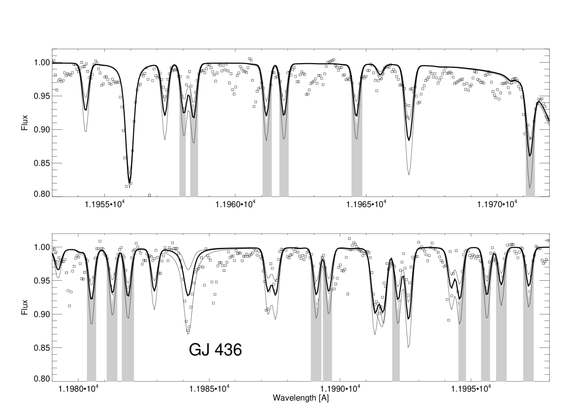
Figure 1: Two selected wavelength regions containing FeH lines, with synthetic and observed spectra for GJ 436. The FeH lines are marked with a grey shade. The thick solid line was calculated using the adopted $T_{\rm eff}$of 3263 K. The upper and lower thin lines are calculated with 200 K higher and lower $T_{\rm eff}$ values, respectively. The observations are represented by open squares.

4.3 Model atmospheres and abundance determination

Table 6: Derived metallicities for our sample and comparison with previous abundance determinations: Bo05: Bonfils et al. (2005a), Be06: Bean et al. (2006a), JA09: Johnson & Apps (2009), SL10: Schlaufman & Laughlin (2010), R10: Rojas-Ayala et al. (2010). The [Fe/H] marked “c” in the JA09 column denotes that this star was not present in their study and we therefore used our collected colours and their provided calibration. Note that the metallicity determination of HD101930B from JA09 is an extrapolation slightly outside the valid range. The metallicities in the Bo05 and SL10 columns are calculated from their respective calibration equations except for the values marked with an ”s” that are spectroscopically determined. The errors quoted for this work are a combination of systematic errors from the uncertainties in atmospheric parameters and the uncertainty from the fitting routine (see Section 4.3).

Target	This work	Bo05	Be06	JA09	SL10	R10
HD101930A	$+$0.20 $\pm$ 0.06
HD101930B	$+$0.09 $\pm$ 0.10	$-$0.16		$+$0.08 c	$-$0.05
GJ105A	$-$0.05 $\pm$ 0.01	$-$0.19 s	$-$0.12
GJ105B	$-$0.06 $\pm$ 0.15	$-$0.15	$-$0.09	$+$0.06 c	$-$0.07	$-$0.04
GJ250A	$-$0.03 $\pm$ 0.05	$-$0.15 s
GJ250B	$-$0.05 $\pm$ 0.05	$-$0.18		$+$0.05 c	$-$0.09
GJ176	$+$0.04 $\pm$ 0.02	$-$0.06		$+$0.18	$+$0.05
GJ317	$+$0.20 $\pm$ 0.14	$-$0.22		$-$0.10	$-$0.21
GJ436	$+$0.08 $\pm$ 0.05	$-$0.05	$-$0.32	$+$0.25	$+$0.08	$+$0.00
GJ581	$-$0.15 $\pm$ 0.03	$-$0.25	$-$0.33	$-$0.10	$-$0.21	$-$0.02
GJ628	$+$0.08 $\pm$ 0.03	$-$0.13		$+$0.12 c	$-$0.02
GJ674	$-$0.11 $\pm$ 0.13	$-$0.28		$-$0.11	$-$0.22
GJ849 P82&84	$+$0.35 $\pm$ 0.10	$+$0.17		$+$0.58	$+$0.37	$+$0.49
GJ876	$+$0.12 $\pm$ 0.15	$+$0.02	$-$0.12	$+$0.37	$+$0.24	$+$0.43

For the metallicity determination we employed the method of fitting synthetic spectra to the observed spectra. The analysis is based on the latest generation of MARCS model atmospheres (Gustafsson et al. 2008). These models give the temperature and pressure distribution in radiative and hydrostatic equilibrium, assuming radiative transport with mixing-length convection in a plane-parallel stellar atmosphere. The formation of dust is not accounted for in the models, as it has been found to be less important in models of early-type M dwarfs (earlier than about M6 or $T_{\rm eff}$ $\gtrsim$ 2600 K; Jones & Tsuji 1997; Tsuji 2002). Our sample includes rather early-type M dwarfs, see Table 1.

We used an improved version of the SME package (Valenti & Piskunov 1996; Valenti & Fischer 2005). This tool performs an automatic parameter optimization using a Levenberg-Marquardt chi-square minimization algorithm. Synthetic spectra are calculated on the fly by a built-in spectrum synthesis code, for a set of global model parameters and specified spectral line data. Starting from user-provided initial values, synthetic spectra are computed for small offsets in different directions for a subset of parameters defined to be “free”. The required model atmospheres are interpolated in the grid of MARCS models available on the MARCS webpage, using an accurate algorithm described in Valenti & Fischer (2005, Section 4.1). Partial derivatives calculated from the corresponding parameter and chi-square values are used to approach the minimum in the chi-square surface. In an independent step from the parameter optimization, the wavelength scale is corrected for any residual velocity shifts by a one-dimensional golden section search. SME also has the option to apply a local fit of the continuum, but we did not use this functionality here. Continuum normalization was instead done during data reduction (see Section 3).

A mask specifies the pixels in the observed spectrum which should be used to determine velocity corrections and to calculate the chi-square. Mask definition is an important step in spectrum synthesis analysis. The radial velocity correction was done in a first step, using most of the observed spectral region and solar metallicity synthetic spectra. This correction was applied to the observed spectra before defining the mask for the metallicity analysis. We placed the mask as consistently as possible for all programme stars to cover the maximum number of spectral lines not affected by blends between different species. Defects in the observed spectra caused by imperfect telluric correction or instrumental effects were masked out, as were the cores of strong lines. For some blended or contaminated lines, a part of the profile was included in the mask if considered useful for the fitting procedure.

The number of available lines in the telluric-free spectra used in the analysis was at maximum 30 in a K dwarf and 23 in an M-dwarf spectrum. The total number of lines included in the analysis of each target spectrum varied slightly due to differences in the data quality, imperfect telluric line removal and other non-physical spectral features. We note that the four potassium lines in our spectra (1169.02, 1176.96, 1177.28, 1252.21 nm) are most likely affected by non-LTE in the solar spectrum. This is suspected from the fact that when we adjusted the $gf$-values for these lines to fit a high-quality solar spectrum, the lines became too strong in the cooler, high-gravity M dwarfs. A discussion on the solar non-LTE effect of these lines can be found in Zhang et al. (2006), where two of the K lines present in our spectra are explored. These authors derive a negative abundance correction for the K lines, meaning that the lines are stronger when calculated in non-LTE than for LTE. Due to the higher densities, collisions may be expected to drive the atmospheres of M dwarfs towards LTE conditions. Although the non-LTE effects in the M dwarfs are probably smaller than in the Sun, they are as yet unknown to us. Hence, we decided not to use the K lines in the analysis and excluded them from our line mask (see Figs. 2 and 3).

There are nine C I lines apparent in the spectra of the Sun and the K dwarfs in our wavelength range. We tried to model these lines using atomic data from Ralchenko et al. (2010), which are based on averaged calculated transition probabilities from two literature sources (Nussbaumer & Storey 1984; Hibbert et al. 1993, using the “velocity” results of the latter), and van der Waals broadening parameters from Barklem et al. (2000). However, the synthetic lines were too weak in the solar spectrum and at the same time somewhat too strong in the K-dwarf spectra, compared to the observations. Hence, we were not able to derive “astrophysical” $gf$-values applicable to both types of stars. We suspect non-LTE effects to be the cause of this problem, which might be spectral-type dependent, in the sense that they are stronger in G-type dwarfs than in K-type dwarfs. This is supported by the fact that all of these lines are high-excitation lines, with lower level energies lying between 7.5 and 8.8 eV. Such levels are easily depopulated by photoionization, which leads to deviations from the LTE approximation. We are not aware of any study of non-LTE effects for the carbon lines in question, and did not include the carbon lines in the analysis.

For all other elements included in our investigation, we do not suspect any non-LTE effects based on the comparisons with the solar spectrum and the K-dwarf spectra. However, we cannot completely exclude any additional non-LTE effects based on our data and models. Unfortunately, non-LTE studies in the infrared region are rare, and investigations have focused on solar-type stars. The study by Allende Prieto et al. (2004) indicates that lines of neutral Fe and Ca might be affected by departures from LTE in the coolest stars of their sample. However, the lowest $T_{\rm eff}$ which they explore is close to 4500 K, and their spectral range extends from about 360 nm to 1 micron. For a review of non-LTE effects in optical spectra of FGK-type stars for a large number of elements see Asplund (2005).

The consistency of the SME solution with the selected surface gravity could be tested using strong lines with well developed wings. While we are not sure about non-LTE effects on potassium line strength we can try to use the shape of these lines for a gravity test. In order to do that we solved for the surface gravity keeping all the other parameters fixed from the optimal solution. The experiment was carried out for one data set for two objects GJ 105B and GJ 628. We find that the surface gravities did not change by more than 0.03 dex confirming that the preset values are consistent with the shapes of strong lines.

We let the overall metallicity, [Fe/H], and the macroturbulence parameter vary and solved for both simultaneously. For the M dwarfs, the unknown microturbulence parameter was set to 1 kms^-1 and line broadening by rotation was neglected, as most of our M dwarfs are known to be relatively slow rotators (see Table 4). As macroturbulence was the only line-broadening parameter, which we included in the fit procedure, the value resulting in the best fit contains contributions from other broadening mechanisms, otherwise unaccounted for, e.g. variations in the instrumental profile, or rotational broadening. The derived values for our programme stars are below 1 kms^-1, except for GJ 876 (1.7 kms^-1), GJ 250A and B ($\approx$2 kms^-1), GJ 674 (3.8 kms^-1 comparable to its $v\sin i$ value in Table 4), and GJ 105B (4.6 kms^-1).

To ensure that we end up in a global minimum when converging to a solution for the best fit, we started from different initial values for the metallicity and plotted the resultant $\chi^{2}$ for each fit as a function of the determined metallicity. This also gave us an estimate of the uncertainties introduced by the fitting routine itself, and was included in the total error calculation. A majority of the lines included in the analysis are weak although some stronger lines are present. We tested the convergence dependence on weak lines as compared to the wings of the stronger lines and found that the strong and weak lines contributed equally to the final $\chi^{2}$ solution. Both strong and weak lines resulted in equal metallicities. We also estimated the Ca abundances for the M dwarfs observed in period 84, where a number of Ca lines are present in the wavelength setup, and find [Ca/Fe] abundances of 0.0–0.1 dex with respect to solar values.

The total uncertainties were computed by perturbing the atmospheric parameters by $\pm$100 K in $T_{\rm eff}$ and $\pm$0.1 dex in $\log g$, and repeating the metallicity fit. The deviations with respect to the adopted [Fe/H] value were then added in quadrature to the uncertainties from the fitting routine itself.

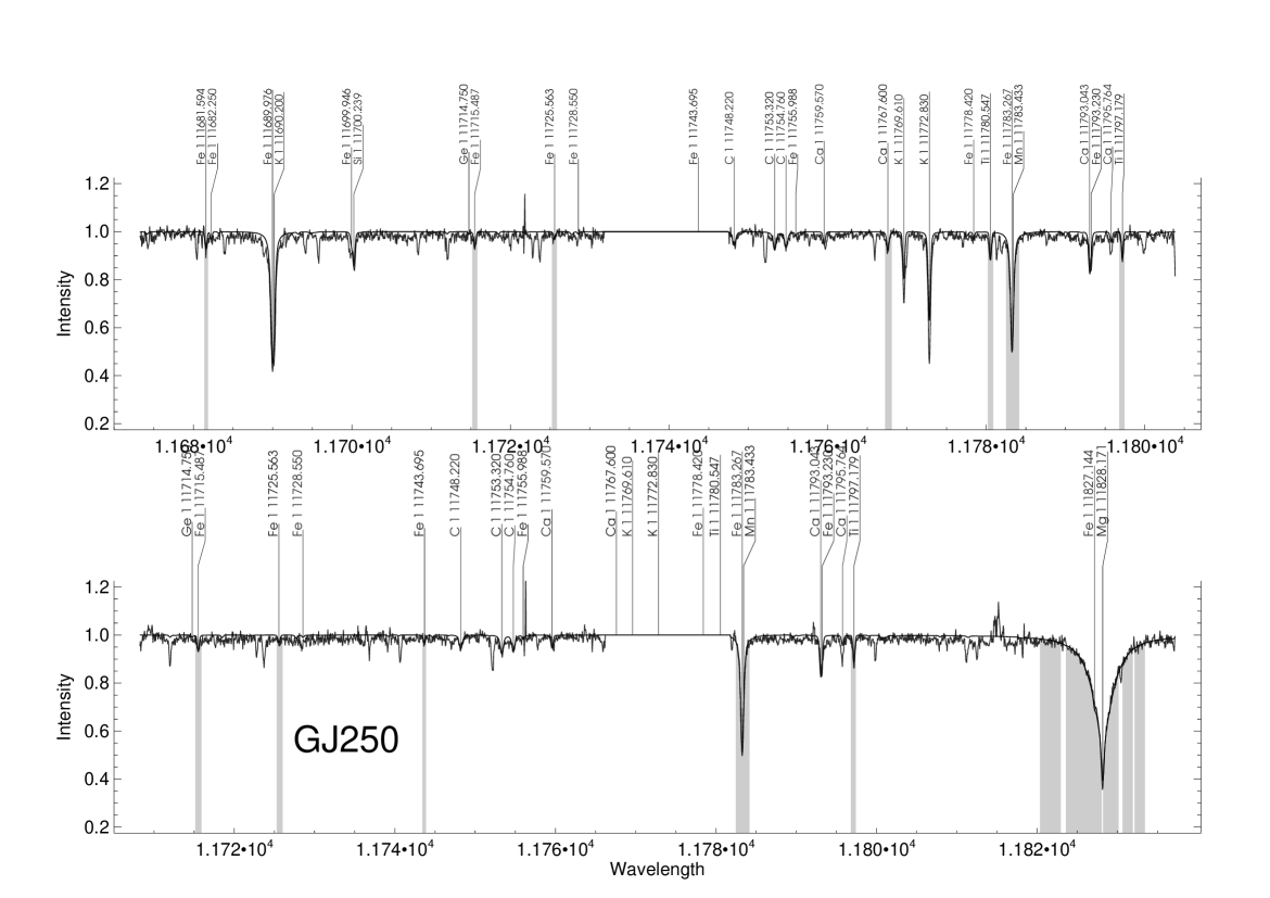
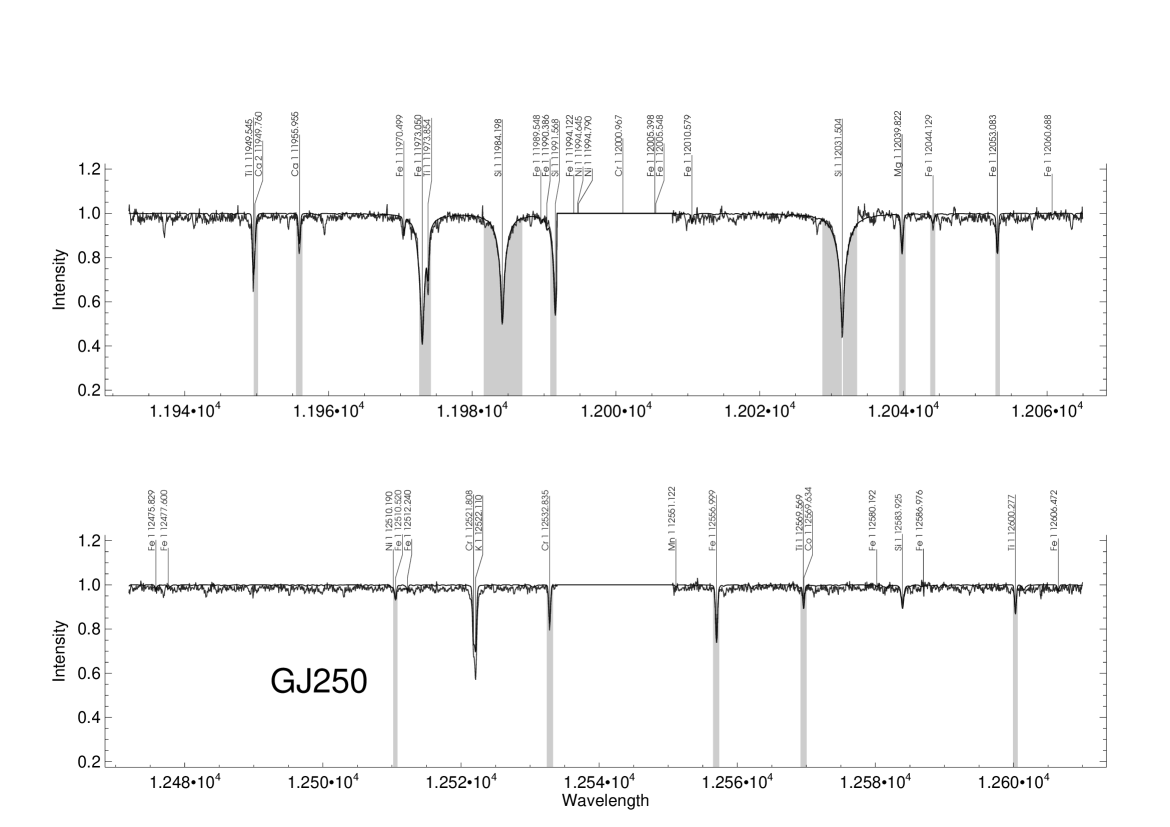
Figure 2: The eight observed wavelength regions in period 82 plotted together with the best fit synthetic spectrum for target GJ250A (primary in double system). The mask used in the metallicity determination is marked with a grey shade.

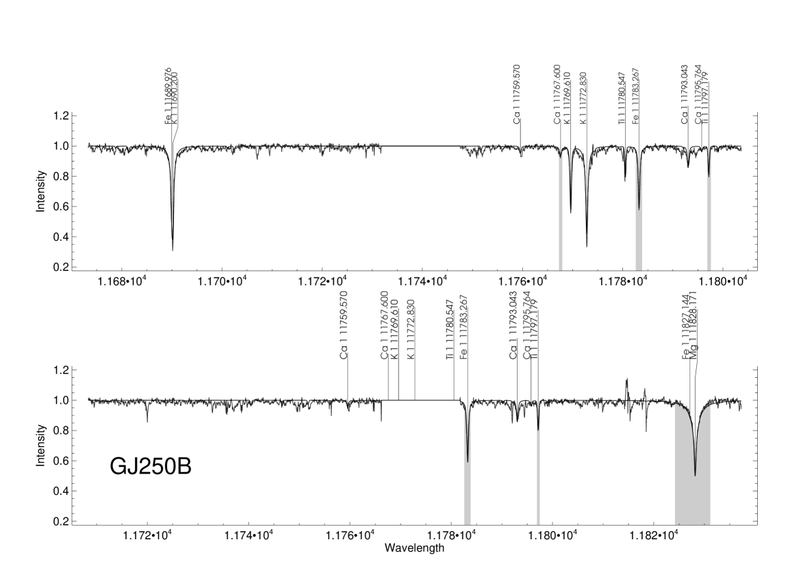
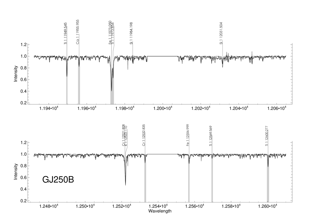
Figure 3: The eight observed wavelength regions in period 82 plotted together with the best fit synthetic spectrum for target GJ250B (secondary in double system). The mask used in the metallicity determination is marked with a grey shade.

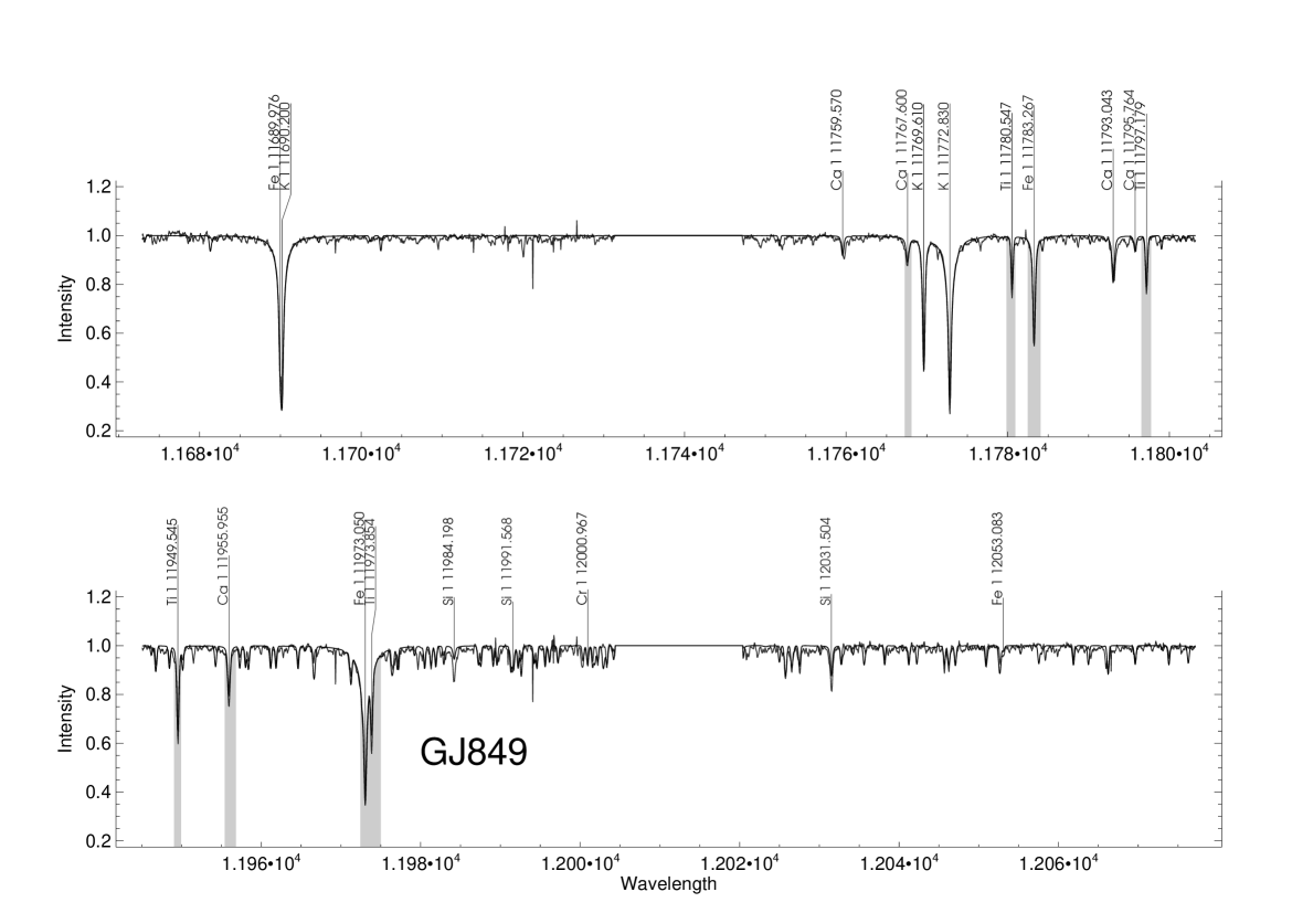
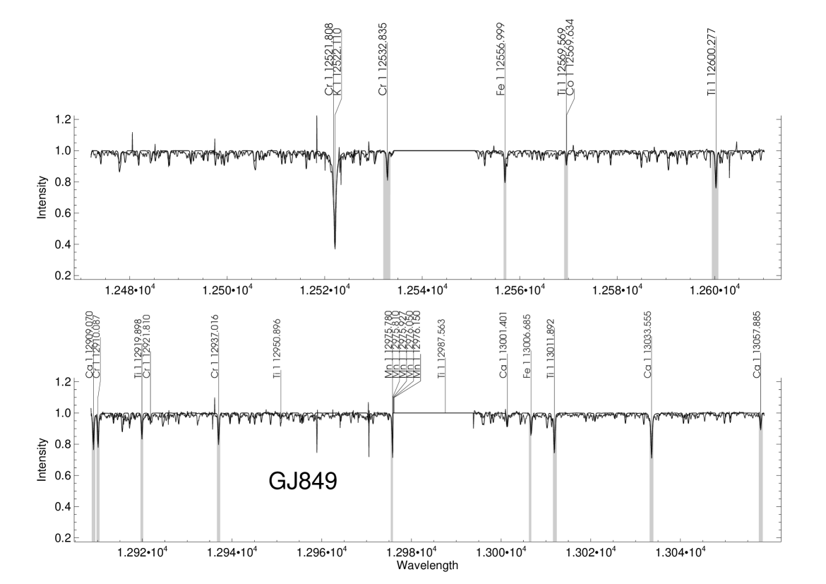
Figure 4: The eight observed wavelength regions plotted together with the best fit synthetic spectrum for one of the coolest targets, GJ849 observed in period 84. The mask used in the metallicity determination is marked with a grey shade.

5 Results and discussion

We have carried out a careful analysis of high-resolution M and K dwarf spectra in the infrared J-band. To calibrate our metallicity scale, three binary systems consisting of a K-dwarf primary and an M-dwarf secondary were observed. The derived metallicities of the binary systems as well as the single M dwarfs can be found in Table 6 and Figure 5. In this table and figure we also list metallicities determined by previous spectroscopic and photometric investigations.

5.1 Binary systems

Stars in binary systems have been formed out of the same molecular cloud and are expected to have the same metallicities. For two of the three binary systems present in this study, we derive very similar metallicities for both components.

The binary system GJ250 AB consists of a K3-dwarf primary and an M2-dwarf secondary. The metallicity determinations for the two stars are consistent within the errors. The synthetic spectra calculated for both stars show good agreement for both weaker as well as stronger lines, including the potassium lines in the M dwarfs that are not included in the derivation of the best fit (see Figs. 2 and 3).

The M dwarf in the GJ105 AB system shows too weak FeH lines in comparison to the calculated spectrum based on the derived photometric effective temperature. We adjusted the temperature by +200 K while solving for [Fe/H] simultaneously as described in Section 4.2. The difference in the determined metallicity of the components in the system was found to be 0.01 dex, which is in agreement with coeval star formation. We note, however, that the best fit synthetic spectrum does not give a satisfactory fit for all atomic lines as the stronger lines tend to be too broad for the established fit. This affect can arise from an incorrect surface gravity, although the potassium line test described above does not support this explanation.

The third binary system, HD101930 AB consists of an early K-dwarf primary (K2) and an early M dwarf (M0-M1). The secondary is the only early M dwarf in our sample and we note that the spectrum shows both features we recognise from the primary, such as strong Si lines, and characteristics seen in the other M dwarfs, such as absent C lines and prominent FeH lines. In a careful study of the best fit synthetic spectrum we noted that a majority of the lines fit rather well except for the strong Si lines and the excluded K lines. We derived a metallicity of 0.09 dex which is 0.11 dex lower than established for the primary of the system. This difference is still on the order of the estimated uncertainties.

5.2 Single M dwarfs

For five of the eight single M dwarfs we derived metallicities for the first time based on high resolution spectroscopy. For the three stars analysed in the optical by Bean et al. (2006a), our metallicities are higher by $\gtrsim$0.2 dex. The recent study using spectroscopic indices by Rojas-Ayala et al. (2010), includes four of our targets and we derived lower metallicities for three of these stars. The photometric calibration by Bonfils et al. (2005a) returns overall lower metallicities than we determined but the calibration is claimed by Johnson & Apps (2009) to produce too low [Fe/H] values. The latter authors corrected for this and we do agree better with this higher metallicity scale. The best agreement we seem to find with Schlaufman & Laughlin (2010), who used a similar technique as Johnson & Apps (2009). After the completion of the present paper, we noted that Neves et al. (2011) recently evaluated the photometric metallicity calibrations of Bo05, JA10 and SL10, and rank the SL10 scale highest. The metallicities derived in our work are shown in Figs. 5 and 6 together with results from the discussed studies. The average differences between our study and those of Schlaufman & Laughlin (2010), Johnson & Apps (2009) and Bonfils et al. (2005a) are 0.09, 0.13 and 0.17, respectively.

6 Conclusions

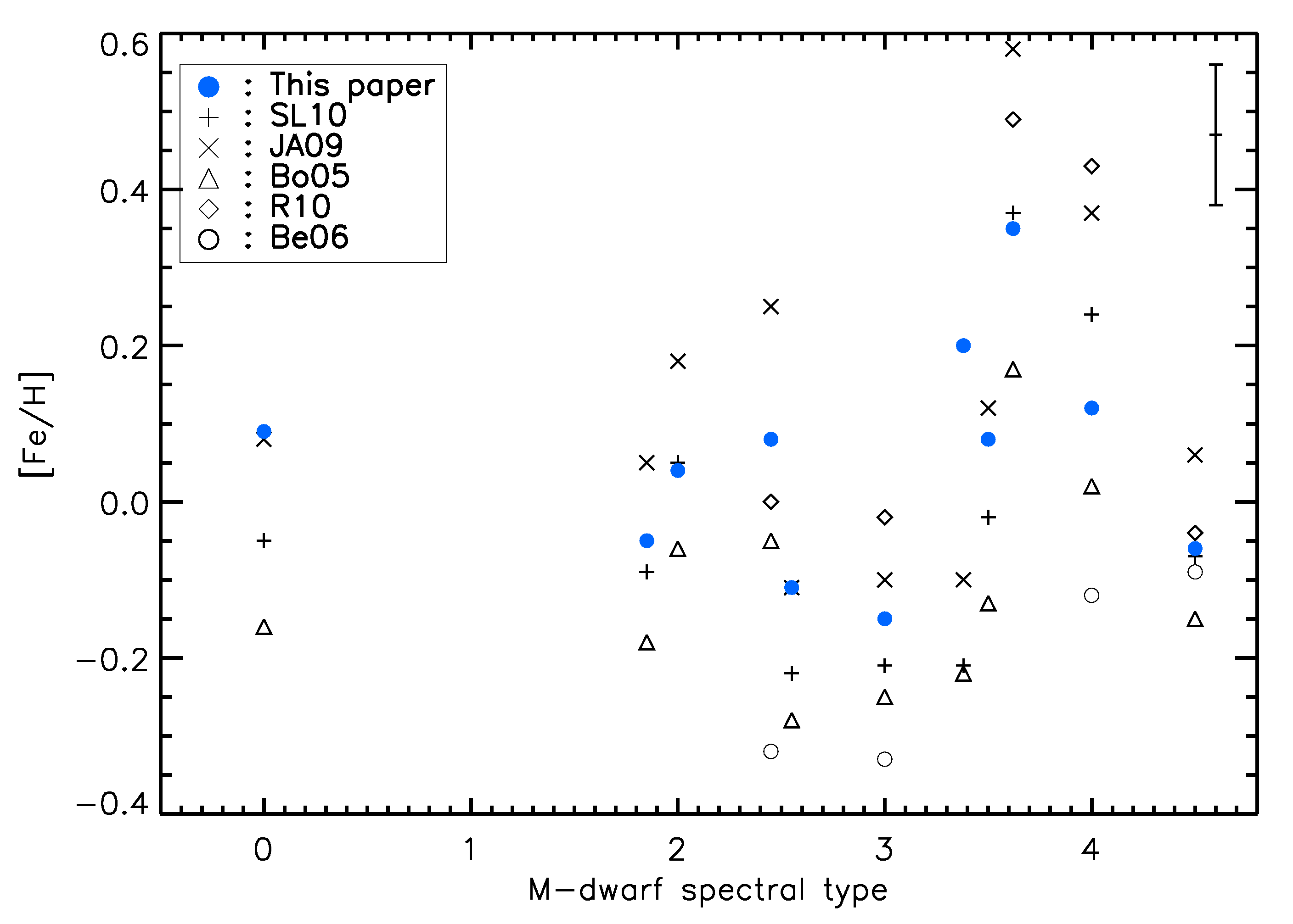
Figure 5: Derived metallicities for our sample in comparison with previous abundance determinations (see Table 6 for references) as a function of spectral type (see Table 1). For an easier presentation the targets with equal spectral types have been slightly shifted horizontally. In the upper right corner we show an error bar indicating the mean error of the metallicities derived in this paper.

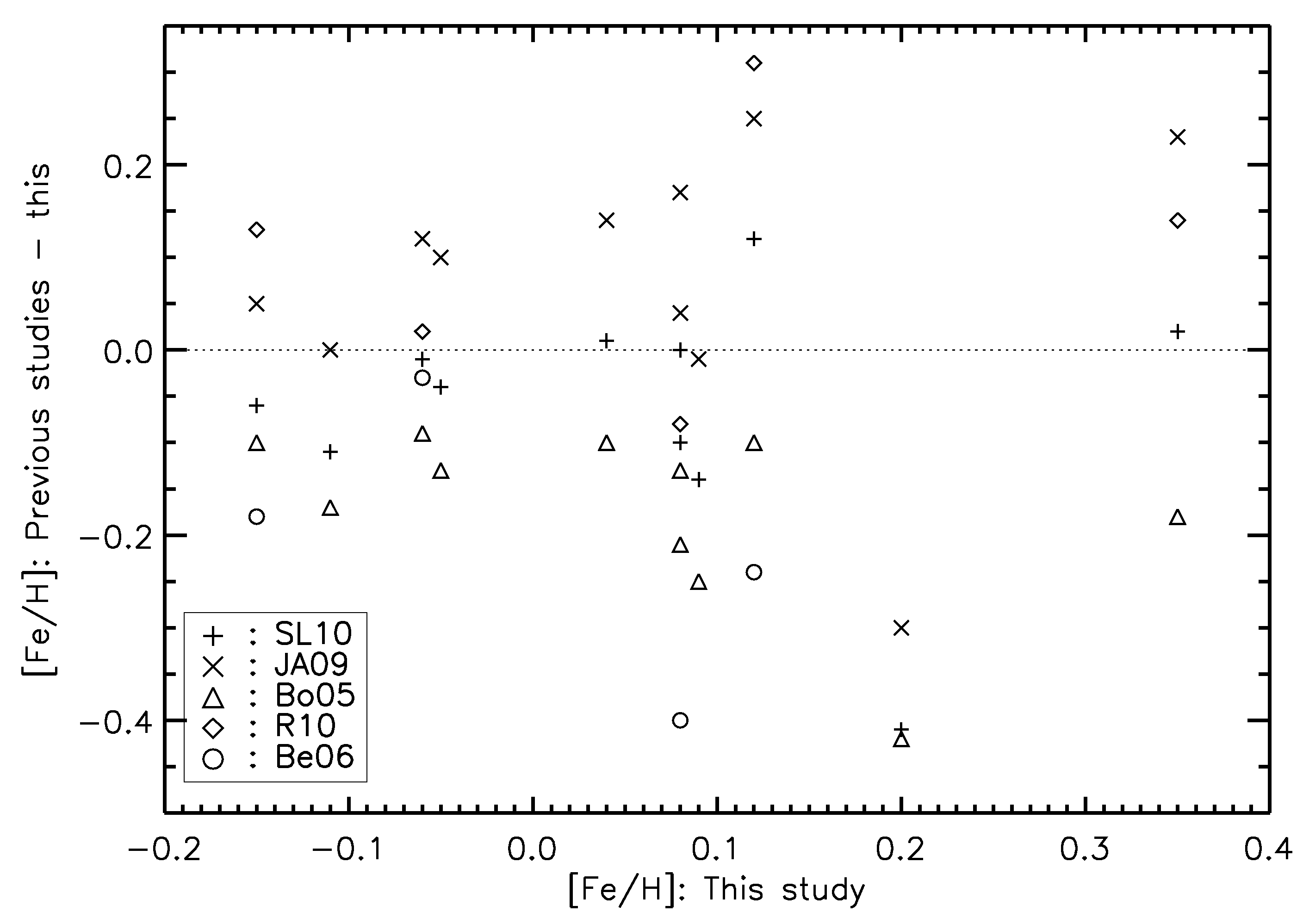
Figure 6: Differences in metallicities for our sample in comparison with previous abundance determinations (see Table 6 for references) as a function of metallicities from this study. A zero-line (dotted) to guide the eye is also plotted.

We have derived a new metallicity scale based on a careful spectroscopic analysis of high-resolution spectra (R$\sim$50,000) observed in the J-band. Previous abundance studies are based on full spectroscopic analyses in the optical regime, low resolution spectroscopic infrared indices as well as purely photometric calibrations. Observations in the infrared J-band have the advantage of few and weak molecular features (FeH) which allows for a precise continuum placement as compared to the optical wavelength regions where the continuum is heavily depressed due to the many and strong TiO lines. We find that we can correct for lines introduced by the Earth’s atmosphere quite succesfully by using a rapidly rotating calibration star, and by applying a carefully determined continuum placement. We verify the accuracy of the atmospheric models involved in the metallicity determination by observing three binary systems that are expected to have the same [Fe/H]. In two of the systems GJ105 AB and GJ250 AB we find that the metallicities agree within 0.01 and 0.02 dex, respectively. In the third binary system, HD101930 AB, we find a discrepancy of 0.11 dex, which is consistent with the derived errors.

We test the convergence of the procedure by starting from different initial guesses and find consistent solutions although some of the cooler objects show a greater spread in the determined metallicity.

Our sample covers a restricted range in $T_{\rm eff}$ (between $\approx$3200 and 3400 K, and a single object at 3900 K), and the extreme metallicities ($<-0.1$ and $>+0.2$) are not well covered. To explore the metallicity scale further, targets with a larger spread in the atmospheric parameters need to be observed, preferrably with an instrument that can cover a larger wavelength range efficiently. Improving the completeness of molecular line lists will improve the accuracy of the metallicity determinations, since there are still a number of unknown molecular blends present.

We conclude that a high-resolution spectroscopic analysis in the near infrared is a reliable method for metallicity determinations in this $T_{\rm eff}$ regime. It is also the only method which will enable the determination of abundances of individual elements in M dwarfs.