Identify Charged Higgs Boson in $W^{\pm}H^{\mp}$ associated production at LHC

Abstract

We investigate the possibility to discover the charged Higgs via $pp\to W^{\pm}H^{\mp}\to l+\displaystyle{\not}E_{T}+b\bar{b}jj$ process at LHC, which suffers from large QCD backgrounds. We optimize the kinematic cuts to suppress the backgrounds, so that the reconstruction of the charged Higgs through hadronic decay is possible. The angular distribution of the b-jet from $H^{\pm}$ decay is investigated as a way to identify the charged scalar from vector bosons.

I Introduction

Understanding electroweak symmetry breaking is one of the driving forces behind the undergoing experiments at the CERN large hadron collider (LHC). In the Standard Model (SM), the fermions and gauge bosons get masses through Higgs mechanism with one weak-isospin doublet Higgs field. Although SM is extremely successful in phenomenology, there are still remaining problems not well understood. Extensions of SM have been considered widely. Two Higgs Doublet Model (2HDM)TDLEE ; SW ; Liu:1987ng ; YLW1 ; Glashow:1976nt ; HW is one of the natural extensions. In this kind of models, the charged Higgs boson ($H^{\pm}$) is of special interest, since its discovery is an unambiguous evidence for an extended Higgs sector. Therefore, the hunt for charged Higgs bosons plays an important role in the search for new physics at LHC.

Currently most of the limits or constraints to the charged Higgs mass are model-dependent. The best model-independent direct limit from the LEP experiments is $m_{H^{\pm}}>78.6$ GeV at 95% C.L.lep:2001ch , assuming only the decay channels $H^{+}\to c\bar{s}$ and $H^{+}\to\tau\nu_{\tau}$. As the charged Higgs will contribute to flavor changing neutral currents at one loop level, the indirect constraints can be extracted from B-meson decays. In Type II 2HDM, the constraint is $M_{H^{\pm}}\gtrsim 350$ GeV for $\tan\beta$ larger than 1, and even stronger for smaller $\tan\beta$ typeII . However, since the phases of the Yukawa couplings in Type III or general 2HDM are free parameters, $m_{H^{\pm}}$ can be as low as 100 GeVBCK .

At hadron colliders, the charged Higgs phenomenology has been studied widely. The main production modes are $gb\rightarrow H^{-}t$ for $m_{H^{\pm}}>m_{t}+m_{b}$ and $gg\rightarrow H^{-}t\bar{b}$ for $m_{H^{\pm}}\lesssim m_{t}-m_{b}$ Barnett ; Bawa ; Borzumati ; Miller ; Alwall:2004xw ; Beccaria:2009my . The preferred decay modes are then $H^{-}\rightarrow b\bar{t}$ and $H^{-}\rightarrow\tau\bar{\nu}_{\tau}$, respectively. Another interesting channel is the $H^{\pm}$ production in association with a $W$ boson, whose leptonic decays can serve as an important trigger for the $W^{\pm}H^{\mp}$ search. This channel can also cover the region $m_{H^{\pm}}\sim m_{t}$. The dominant channels for $W^{\pm}H^{\mp}$ production are $b\bar{b}\rightarrow W^{\pm}H^{\mp}$ at tree level and $gg\rightarrow W^{\pm}H^{\mp}$ at one-loop level. $W^{\pm}H^{\mp}$ production at hadron colliders in Type II 2HDM and other 2HDMs has been studied in Kniehl ; Dicus ; Brein ; Asakawa ; Eriksson ; Bao:2010sz . It is found that, due to the large negative interference term between the triangle- and box-type quark-loop Feynman diagrams, the gluon-fusion cross section in MSSM is quite small. The NLO-QCD and SUSY-QCD corrections to $b\bar{b}$ annihilation amplitude in MSSM are all about 10%Zhao:2005mu ; Gao:2007wz . As has studied in Kniehl ; Moretti:1998xq , the hadronic decay channel of $H^{\pm}$ suffers from large QCD backgrounds, which overwhelm the charged Higgs signal over the heavy mass range that can be probed at LHC. In this paper, we optimize the kinematic cuts of the final state. The signal-background ratio is improved so that the resonance reconstruction is possible. Once the resonance of $b\bar{t}~{}(t\bar{b})$ is detected at LHC, its spin should be determined. We investigate the angular distribution of the b-jet with respect to the beam direction. It is found that such distribution is useful to identify the charged scalar from vector bosons.

This paper is organized as follows. In section II, the corresponding theoretical framework is briefly introduced. Section III is devoted to the numerical analysis of $W^{\pm}H^{\mp}$ production and the related SM backgrounds. In section IV, the angular distributions of b-jet are investigated to identify the scalar from vector bosons. Finally, a short summary is given.

II Theoretical framework for Charged Higgs

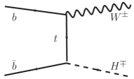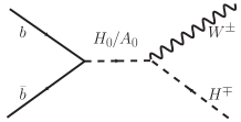
(a)	(b)

Figure 1: Feynman diagrams for $W^{\pm}H^{\mp}$ production at partonic level.

The scalar sector of SM is not yet confirmed by experiments and it is possible to extend the Higgs structure to two Higgs doublets. For example, it has been shown that if one Higgs doublet is needed for the mass generation, an extra Higgs doublet is necessary for the Spontaneous $CP$ violationTDLEE . In 2HDMs, after the spontaneous symmetry breaking, there remain five physical Higgs scalars, i.e., two neutral $CP$-even bosons $h_{0}$ and $H_{0}$, one neutral $CP$-odd boson $A_{0}$, and two charged bosons $H^{\pm}$. In this work we aim to study the charged Higgs phenomenology and choose the Type II Yukawa couplings as the working model,

$$-\mathcal{L} = -\cot\beta\frac{m^{u}}{v}\bar{u}_{L}(H+iA)u_{R}-\cot\beta\frac{m^{u}}{v}\bar{u}_{R}(H-iA)u_{L}$$ (1)

$$+\tan\beta\frac{M^{d}}{v}\bar{d}_{L}(H-iA)d_{R}+\tan\beta\frac{M^{d}}{v}\bar{d}_{R}(H+iA)d_{L}$$

$$-\sqrt{2}\cot\beta\frac{M^{u}}{v}V_{ud}^{{\dagger}}\bar{d}_{L}H^{-}u_{R}-\sqrt{2}\tan\beta\frac{M^{d}}{v}V_{ud}^{{\dagger}}\bar{d}_{R}H^{-}u_{L}$$

$$-\sqrt{2}\cot\beta\frac{M^{u}}{v}V_{ud}\bar{u}_{R}H^{+}d_{L}-\sqrt{2}\tan\beta\frac{M^{d}}{v}V_{ud}\bar{u}_{L}H^{+}d_{R}.$$

The Yukawa couplings are related to the fermion masses, which indicates that the dominant production processes for the charged Higgs associated with a $W$ boson at hadron collider are $b\bar{b}$ annihilation at tree-level and gluon fusion at one loop level. The $b\bar{b}$ annihilation is overwhelming for $\tan\beta>1$Kniehl , while large $\tan\beta$ is favored by $B$ meson rare decaysHewett:1992is ; Barger:1992dy ; Bertolini:1990if . In this work we investigate the properties of charged Higgs with large $\tan\beta$ in $b\bar{b}$ annihilation process. The Feynman diagrams are shown in Fig. 1. The corresponding invariant amplitude square averaged over the spin and color of initial partons is given by

$$|{\cal M}|^{2} = \left.\frac{G_{F}^{2}{\hat{s}}}{6}\right\{2m_{b}^{2}\tan^{2}\beta[({\hat{s}}-m_{W}^{2}-m_{H}^{2})^{2}-4(m_{W}m_{H})^{2}](|G_{H_{0}}|^{2}+|G_{A_{0}}|^{2})$$ (2)

$$+ [m_{b}^{2}\tan^{2}\beta({\hat{s}}{\hat{t}}^{2}+2{\hat{t}}{\hat{u}}m_{W}^{2}-2m_{W}^{4}m_{H}^{2})+m_{t}^{4}\cot^{2}\beta({\hat{t}}{\hat{u}}+2{\hat{s}}m_{W}^{2}-m_{W}^{2}m_{H}^{2})]\frac{4}{{\hat{s}}({\hat{t}}-m_{t}^{2})^{2}}$$

$$+ \left.m_{b}^{2}\tan^{2}\beta({\hat{t}}^{2}+{\hat{t}}{\hat{u}}-2m_{W}^{2}m_{H}^{2})\frac{1}{{\hat{t}}-m_{t}^{2}}Re(G_{H_{0}}+G_{A_{0}})\right\},$$

where $\hat{s}=(p_{b}+p_{\bar{b}})^{2},~{}\hat{t}=(p_{b}-p_{W})^{2},~{}\hat{u}=(p_{b}-p_{H})^{2}$ are the Mandelstam variables and $G_{F}$ is the Fermi constant. The Higgs propagator functions are

$$G_{H_{0},A_{0}}=\frac{1}{\hat{s}-m_{H_{0},A_{0}}^{2}+i\Gamma_{H_{0},A_{0}}m_{H_{0},A_{0}}},$$ (3)

where $\Gamma_{H_{0},A_{0}}$ are the higgs widths which are obtained with HDECAYDjouadi:1997yw package.

III $W^{\pm}H^{\mp}$ Production and Corresponding backgrounds

Figure 2: The total cross section as a function of $m_{H^{\pm}}$ for $pp\to W^{\pm}H^{\mp}$ process at (a) $\sqrt{s}=7$ TeV and (b) $\sqrt{s}=14$ TeV.

The total cross section for the $pp\to W^{\pm}H^{\mp}$ process can be written as follows

$$\sigma=\int f_{b}(x_{1})f_{\bar{b}}(x_{2})\hat{\sigma}(x_{1}x_{2}s)dx_{1}dx_{2},$$ (4)

where $\sqrt{s}$ is the proton-proton center of mass energy, $\hat{\sigma}$ is the partonic level cross section of $b\bar{b}\to W^{\pm}H^{\mp}$, and $f_{q}(x_{i})$ is the parton distribution function (PDF). In our numerical calculations, we employ CTEQ6L1Pumplin:2002vw for PDF, and set $V_{tb}=1$, $M_{W}=80.4$ GeV, and $m_{t}=172.9$ GeV. In Fig. 2, the total cross sections are shown as a function of charged Higgs mass for $\tan\beta=10$, 30, and 50 at LHC. The cross section increases with $\tan\beta$. Supposing the luminosity to be $10~{}fb^{-1}$ at $\sqrt{s}=7$ TeV, one can notice that it is difficult for the charged Higgs associated with a $W$ boson to be detected when its mass is above 600 GeV even for $\tan\beta=50$. It is easier for the charged Higgs boson to be observed at $\sqrt{s}=14$ TeV. Therefore in this work we focus on investigating the charged Higgs associated with a $W$ boson in the following processes

$$pp \to W^{-}H^{+}\to W^{-}t\bar{b}\to l^{-}\nu b\bar{b}jj,$$ (5)

$$pp \to W^{+}H^{-}\to W^{+}\bar{t}b\to l^{+}\nu b\bar{b}jj$$

at $\sqrt{s}=14$ TeV with $\tan\beta=30$.

Figure 3: (a) The transverse momentum distributions of the jets ($j_{1},j_{2},j_{3},j_{4}$) with $p_{Tj_{1}}>p_{Tj_{2}}>p_{Tj_{3}}>p_{Tj_{4}}$ for $m_{H^{\pm}}=500$ GeV at $\sqrt{s}=14$ TeV. (b) The transverse momentum distribution of the charged lepton (solid line) and the missing transverse energy $\displaystyle{\not}E_{T}$ distribution (dashed line). (c) The minimal angular separation distributions between jets (solid line) and that between jets and the charged lepton (dashed line).

Figure 4: The $b\bar{b}jj$ invariant mass distributions.

To be more realistic, the simulation at the detector is performed by smearing the leptons and jets energies according to the assumption of the Gaussian resolution parametrization

$$\frac{\delta(E)}{E}=\frac{a}{\sqrt{E}}\oplus b,$$ (6)

where $\delta(E)/E$ is the energy resolution, $a$ is a sampling term, $b$ is a constant term, and $\oplus$ denotes a sum in quadrature. We take $a=5\%$, $b=0.55\%$ for leptons and $a=100\%$, $b=5\%$ for jets respectivelyAad:2009wy .

The transverse momentum distributions for the four jets are shown in Fig. 3 (a). In Fig. 3 (b), the transverse momentum distribution for the charged lepton and the missing transverse energy ($\displaystyle{\not}E_{T}$) distribution are displayed. In order to identify the isolated jet (lepton), we define the angular separation between particle $i$ and particle $j$ as

$$\Delta R_{ij}=\sqrt{\Delta\phi_{ij}^{2}+\Delta\eta_{ij}^{2}},$$ (7)

where $\Delta\phi_{ij}=\phi_{i}-\phi_{j}$ and $\Delta\eta_{ij}=\eta_{i}-\eta_{j}$. $\phi_{i}$ ($\eta_{i}$) denotes the azimuthal angle (rapidity) of the related jet (or lepton). The corresponding distributions for $\Delta R=min(\Delta R_{ij})$ are shown in Fig. 3 (c).

The momentum of the neutrino can be reconstructed from the $W$ mass, missing transverse momentum and neutrino mass, i.e., the neutrino momentum is obtained by solving the following equations

$${\bf p}_{\nu T} = -({\bf p}_{lT}+\sum{\bf p}_{jT}),$$

$$m_{W}^{2} = (p_{\nu}+p_{l})^{2},\;p_{\nu}^{2}=0,$$ (8)

where ${\bf p}_{iT}$ is the transverse momentum of the corresponding particle and $p_{\nu}$ ($p_{l}$) is the four-momentum of neutrino (charged lepton). We veto the event if no solution can be found.

In our analysis, all the hadronic jets are from the charged Higgs boson decay. As a result, the invariant mass of these jets can be used to reconstruct the charged Higgs boson mass. The distributions $d\sigma/dM_{jjjj}$ for various charged Higgs mass are shown in Fig. 4.

Based on the above discussion, we employ the basic cuts (referred as cut I)

$$p_{lT}>20~{}GeV,~{}p_{jT}>30~{}GeV,~{}\displaystyle{\not}E_{T}>20~{}GeV,$$

$$|\eta_{l}|<2.5,~{}|\eta_{j}|<3.0,~{}\Delta R_{jj(lj)}>0.4.$$ (9)

For the processes Eq. (12) with final state $l+\displaystyle{\not}E_{T}+b\bar{b}jj$, the dominant SM backgrounds are $t\bar{t}$, $t\bar{t}W$, $t\bar{t}Z$, $WZjj$, $WWjj$ and $Wjjjj$, which are generated with the MadGraphmadgraph and Alpgenalpgen . In the $W^{\pm}H^{\mp}$ production processes, four jets are from the charged Higgs decay, and three of them are from top quark decay. Therefore to purify the signal, one can require the invariant mass of final jets to be around the charged Higgs mass, and one top quark is reconstructed by three jets. Since $t\bar{t}$ is one of the predominant backgrounds, one can veto $t\bar{t}$ events if the second top quark can be reconstructed. Such kinds of invariant mass cut (referred as cut II) are

$$|M_{jjjj}-m_{H^{\pm}}|\leq 30~{}GeV,~{}~{}|M_{jjj}-m_{t}|\leq 20~{}GeV~{}and~{}~{}|M_{jl\nu}-m_{t}|\geq 20~{}GeV.$$ (10)

In order to further purify the signal, we apply a cut on the invariant mass for all of the visible particles

$$M_{jjjjl}=\sqrt{(\sum p_{j}+p_{l})^{2}}>1.5m_{H^{\pm}}$$ (11)

together with one b-tagging (referred as cut III).

The cross sections for signal after each cut are listed in table 1. We find that after all cuts, there is about 1 $fb$ left for the signal process around $m_{H^{\pm}}=500$ GeV, and the backgrounds are suppressed significantly. In table 2, we list the event numbers for the signal and background processes survived after all cuts with the integral luminosity of $300~{}fb^{-1}$ at $\sqrt{s}=14$ TeV. The significance for the signal to background can reach above three sigma for $m_{H^{\pm}}\geq 400$ GeV. As an example, we choose $m_{H^{\pm}}=$ 500 GeV for the investigation in section IV.

$m_{H^{\pm}}$(GeV)	No cuts	Cut I	Cut I+II	Cut I+II+III
300	105	6.37	3.33	1.43
400	49.7	4.41	2.05	1.11
500	25.7	2.83	1.20	0.72
600	14.1	1.81	0.70	0.45
800	4.90	0.77	0.26	0.18
1000	1.93	0.35	0.10	0.07

Table 1: The cross section of the signal process at $\sqrt{s}=14$ TeV in unit of $fb$.

$m_{H^{\pm}}(GeV)$	300	400	500	600	800	1000
$W^{\pm}H^{\mp}$	429	333	216	135	54	21
$t\bar{t}$	14640	3360	696	231	$<$1	$<$1
$t\bar{t}W$	24	9	3	2	$<$1	$<$1
$t\bar{t}Z$	30	6	$<$1	$<$1	$<$1	$<$1
$WZjj$	69	$<$1	$<$1	$<$1	$<$1	$<$1
$WWjj$	120	117	$<$1	$<$1	$<$1	$<$1
$Wjjjj$	20940	5970	$<$1	$<$1	$<$1	$<$1
$S/B$	0.01	0.03	0.31	0.57	$>$9	$>$3.5
$S/\sqrt{B}$	2.27	3.42	8.15	8.77	$>$22	$>$8.57

Table 2: The event numbers after all cuts for the signal and backgrounds with a integral luminosity of $300~{}fb^{-1}$ at $\sqrt{s}=14$ TeV. The signal$-$background ratio and the significance are given.

IV Identify $H^{\pm}$ from charged vector bosons

The reconstruction of the resonance from $b\bar{t}~{}(t\bar{b})$ final states can straightforward lead to the conclusion that a new charged boson is detected. However, many theories beyond SM also predict the existence of new heavy charged vector bosons (e.g. $W^{\prime\pm}$) which can decay to $b\bar{t}~{}(\bar{tb})$. It can not be ignored to identify the scalar from the vector bosons with the identical final state. We study the following processes

$$pp \to W^{-}W^{\prime+}\to W^{-}t\bar{b}\to l^{-}\nu b\bar{b}jj,$$ (12)

$$pp \to W^{+}W^{\prime-}\to W^{+}\bar{t}b\to l^{+}\nu b\bar{b}jj.$$

The corresponding transverse momentum distributions and $b\bar{b}jj$ invariant mass are similar to Fig. 3 and Fig. 4. Hence a proper observable has to be found to represent the spin of the new particle, which is another main aim of this paper.

Figure 5: The angular distribution of bottom quark in the (a) $W^{\pm}H^{\mp}$ process and (b) $W^{\pm}W^{\prime\mp}$ process at LHC for $m_{(H^{\pm},W^{\prime\pm})}=500$ GeV. Solid, dashed and dotted lines respectively stand for the distributions through $W_{L}^{\prime\pm}$, $W_{R}^{\prime\pm}$ and $W_{V}^{\prime\pm}$. The symbols $W_{L}^{\prime\pm}$ ($W_{R}^{\prime\pm}$) and $W_{V}^{\prime\pm}$ respectively denote the vector bosons participated in left (right) handed and pure vector type interactions.

Figure 6: The angular distribution of b-jet in the (a) $W^{\pm}H^{\mp}$ process and (b) $W^{\pm}W^{\prime\mp}$ process at LHC after the detector simulation and through all cuts, Solid, dashed and dotted lines respectively stand for the distributions through $W_{L}^{\prime\pm}$, $W_{R}^{\prime\pm}$ and $W_{V}^{\prime\pm}$. The symbols are similar to Fig. 5.

Taking into account that the scalar particle is different from the vector ones in the angular distribution of their decay products, we can define the angle $\theta$ as follows

$$\cos\theta=\frac{{\bf p}_{b}^{*}\cdot{\bf p}}{|{\bf p}_{b}^{*}||{\bf p}|},$$ (13)

where ${\bf p}$ is the 3-momentum of one of the initial proton in the laboratory frame, and ${\bf p}_{b}^{*}$ is the 3-momentum of the b-jet which is not decay from top (anti-)quark in the $H^{\pm}$ (or $W^{\prime\pm}$) rest frame. The distributions $\frac{d\sigma}{\sigma d\cos\theta}$ related to $H^{\pm}$ and $W^{\prime\pm}$ without any cuts are shown in Fig. 5. The bottom (anti-)quark in $H^{\pm}$ rest frame is isotropic, and has no correlation with the proton moving direction. However, if the new charged particle is a vector ($W^{\prime\pm}$), the ${\bf p_{b}^{*}}$ is not isotropic any more. The distribution is sensitive to the chiral couplings. Such chiral couplings of $W^{\prime\pm}$ have also been studied in other processesBao:2011nh ; Gopalakrishna:2010xm . Fig. 6 shows the corresponding b-jet angular distributions after the smearing and the kinematic cuts in section III. One can find that the curve for $H^{\pm}$ is slightly distorted by the kinematic cuts, which does not change the fact that the distributions corresponding to the scalar and the vector bosons are characteristically different. To characterize such difference, we employ the function

$$f(\cos\theta)=\frac{1}{2+\frac{2}{3}A}(1+A\cos^{2}\theta)$$ (14)

to fit the curves in Fig. 5 and 6. The values of $A$ are listed in table 3. Obviously, $A$ is different for scalar and vector bosons before or after all cuts. Therefore, the investigation of the angular distribution and the characteristic quantity $A$ is helpful to discriminate the charged scalar from the vector bosons.

	$H^{\pm}$	$W_{L}^{\prime\pm}$	$W_{R}^{\prime\pm}$	$W_{V}^{\prime\pm}$
No cuts	0	0.69	0.28	0.65
Cut I+II+III	-0.13	0.66	0.14	0.60

Table 3: The values of $A$ from fitting the curves in Fig. 5 and 6 with the function Eq. (14).

V Summary

We investigate the possibility of detecting charged Higgs production in association with $W$ boson via $pp\to W^{\pm}H^{\mp}\to l+\displaystyle{\not}E_{T}+b\bar{b}jj$ at LHC. We apply the resonance reconstruction (cut II) and resonance mass dependence (cut III) to suppress the QCD backgrounds. It is found that with $300~{}fb^{-1}$ integral luminosity at $\sqrt{s}=14$ TeV, the signal can be distinguished from the backgrounds for the charged Higgs mass around 400 GeV or larger. If a new resonance particle is observed, one of the key question is to identify its spin. We study the angular distributions for the charged Higgs and the representative vector bosons ($W^{\prime\pm}$) with various chiral couplings. From the angular distributions and the characteristic quantity $A$ the scalar can be distinguished from the vector bosons. The above analysis can be applied to discriminate the scalar from the vector bosons once the new resonance particle produced in association with a vector gauge boson (e.g. $W$ or $Z$) is discovered at LHC.