Imprints of Cosmic Phase Transition in Inflationary Gravitational Waves
Abstract
We discuss the effects of cosmic phase transition on the spectrum of primordial gravitational waves generated during inflation. The energy density of the scalar condensation responsible for the phase transition may become sizable at the epoch of phase transition, which significantly affects the evolution of the universe. As a result, the amplitudes of the gravitational waves at high frequency modes are suppressed. Thus the gravitational wave spectrum can be a probe of phase transition in the early universe.
Spontaneous symmetry breaking (SSB) often plays very important role in high energy physics. For the construction of the standard model of particle physics, which is currently the most successful model of high energy phenomena, the SSB of due to the Higgs mechanism (i.e., the electroweak symmetry breaking) is crucial. In addition, at the scale of the quantum chromodynamics (QCD), chiral symmetry breaking also occurs. If we consider various models of physics beyond the standard model, SSBs may occur at higher energy scales. For example, if the strong CP problem is solved by the Peccei-Quinn (PQ) mechanism Peccei:1977hh , the PQ symmetry breaking should happen at the PQ scale. In grand unified theories (GUTs) Georgi:1974sy , the symmetry breaking of occurs at the GUT scale (where is the GUT gauge group). In supersymmetric models, the supersymmetry breaking terms are expected to arise due to the spontaneous breaking of supersymmetry.
The SSBs in the framework of the standard model, i.e., the electroweak symmetry breaking and the chiral symmetry breaking in QCD, may be well understood in the future by experimental data (in particular, by the LHC result), lattice simulation, and so on. However, it is difficult to study the SSBs in models beyond the standard model because their energy scales are too high to be reached by collider experiments. Thus, the physics related to those SSBs at high energy scales are hardly probed by the existing methods.
If we consider cosmology, there should exist in the past a period of cosmic phase transition related to the SSB. In particular, in a period around the phase transition, the expansion of the universe may be significantly affected by the energy density of the fields which cause the SSB, which results in a significant deviation from the radiation-dominated universe. In the following, we will show that information of such an early universe may be imprinted in the spectrum of primordial gravitational waves (GWs) generated during inflation. This is because the GW spectrum is sensitive to the expansion history of the universe Seto:2003kc ; Smith:2005mm ; Boyle:2005se ; Nakayama:2008ip ; Kuroyanagi:2008ye ; Nakayama:2009ce ; Kuroyanagi:2011fy . Importantly, the GW spectrum may be studied at future experiments such as DECIGO Seto:2001qf and/or BBO gr-qc/0506015 .
In this letter, we discuss the possibility of studying cosmic phase transition in the early universe by using GW. We will show that the evolution of the amplitudes of GW may be significantly affected if phase transition happened in the early epoch and hence the information on the SSB may be extracted from the spectrum of GW.
Let us first discuss how the amplitudes of GWs evolve in the expanding universe. The tensor perturbation of the metric, which corresponds to the degrees of freedom of the GW, is defined as
| (1) |
where is the line element, and the indices and run . The tensor perturbation satisfies transverse and traceless conditions, . Thus, there are two physical degrees of freedom (for a fixed value of the momentum), which we denote by and . In the following discussion, it is convenient to work in the momentum space, so we define the Fourier amplitude of as
| (2) |
where is the reduced Planck scale, and is the polarization tensor which satisfies . Then, satisfies
| (3) |
where the “dot” denotes the derivative with respect to time, and . Here, we neglect the anisotropic stress which is irrelevant for the present study. Although we will numerically follow the evolution of the GW amplitudes, it is instructive to shortly discuss the qualitative behavior of the solution of Eq. (3). When (out of horizon), the last term of the left-hand side is irrelevant and hence stays (almost) constant. On the contrary, once the mode enters the horizon (i.e., ), is under oscillation; in this case, and are approximately proportional to and , respectively, where denotes the average for the time scale much longer than the oscillation time (but shorter than cosmic time).
During inflation, the quantum fluctuation of the GW determines the initial value of . The present GW spectrum per log wavenumber interval for (where and are comoving wavenumbers of modes which enter the horizon at the time of electroweak phase transition and reheating after inflation, respectively) is given by
| (4) |
Here, is the tensor-to-scalar ratio in units of and
| (5) |
where denotes the temperature at which the mode enters the horizon, and denote the effective number of relativistic degrees of freedom for the energy density and the entropy density, respectively, with subscript being for the present value. In addition, is the pivot scale and is the tensor spectral index, which is given by in standard inflation models. Thus the scale dependence of the primordial GW spectrum is very weak as long as is small enough. Hereafter, we neglect the scale dependence for simplicity.
Now let us discuss how the universe expands in the period of cosmic phase transition. During the cosmic phase transition, the expectation value of the order parameter changes from zero to a finite value due to thermal effects. The detail of the phase transition depends on the physics in the SSB sector. In the present study, we model the SSB sector simply by introducing a scalar field which plays the role of the order parameter. With and being (real) scalar fields, we consider the following scalar potential,
| (6) |
where and are coupling constants while is the vacuum expectation value of .#1#1#1 Problematic domain wall formations are avoided if one regards as a radial part (absolute value) of the complex scalar field, which triggers the SSB of a continuous symmetry, such as U(1). Cosmic strings in association with the SSB of U(1) are not harmful for GeV. Here, represents the scalar field responsible for the cosmic phase transition; () corresponds to the symmetric (broken) phase, while represents the degrees of freedom in thermal bath (with temperature ).
With being in thermal bath, the free energy of acquires a term proportional to around . Thus, in the early universe with high enough temperature, the symmetry is expected to be restored. As the temperature decreases, the negative mass-squared term in the (zero-temperature) scalar potential wins over the thermal mass term, and the SSB takes place. Here, we expect that the evolution of is well governed by the following equation,
| (7) |
where is the expansion rate of the universe, is the decay rate of , and the “dash” denotes derivative with respect to . In addition, is the potential of in thermal bath, which we evaluate as , where (with being density matrix) is thermal average of the operator . We consider the case where the time scale of the change of is much smaller than that of cosmic expansion. Thus, we take , where is the Hamiltonian in -sector to calculate .
We evaluate the thermal average by approximating as a free scalar field with the mass squared of and obtain
| (8) | |||||
where .#2#2#2One may estimate the expectation value of by minimizing the free energy. In the present analysis, we approximate that the phase transition occurs when the curvature of the potential at becomes zero. With such an approximation, results of free-energy and our procedures agree because the thermal mass of the scalar field obtained in two procedures are the same. For the following discussion, it is instructive to expand the potential around to find
| (9) |
where
| (10) |
Thus, the curvature at changes its sign at .
Because we are interested in the case where , the oscillation of decays away with the time scale much faster than the cosmic expansion. Thus, we can approximate that follows the temporal minimum of . Even so, an accurate understanding of the evolution of is not straightforward because, in some period, has two minima. In particular, at the temperature just above , is not the absolute minimum of the potential, and hence the phase transition may proceed with a tunneling from to the absolute minimum Callan:1977pt . Whether the phase transition completes via the first or second order phase transition depends on the parameters in the model. For , the second order phase transition precedes the first order one. For , the first order phase transition may take place at the temperature . In either case, we simply approximate that the phase transition occurs at the time when the cosmic temperature becomes for the first time. In addition, because the position of the true minimum of the potential at well agrees with that at , we approximate the energy density of the sector as
| (13) |
where is the time of the phase transition.
With the above approximation, the evolution of the scale factor is governed by
| (14) |
where is the energy density of the radiation component; it evolves as
| (15) |
and is related to the cosmic temperature as , with being the effective number of massless degrees of freedom. In our analysis, we take the standard-model value of , which is . Although may also contribute to , such a contribution is so small that we can safely neglect it.
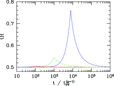
In Fig. 1, we plot the product of the time and the expansion rate as a function of for several values of . (In the plot, is normalized by , which is the time of the phase transition for the case of , to make the figure independent of .) The product is equal to if the universe is dominated by radiation. We can see that the evolution of the universe at deviates from that of radiation-dominated universe as becomes smaller. This behavior can be easily understood from the relation . For smaller , the potential energy of at the origin tends to dominate the universe before the phase transition. In the small limit, a brief period of inflation takes place Lyth:1995ka .
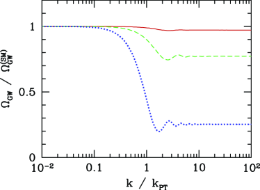
Once the evolution of the scale factor is understood, we can easily solve Eq. (3) to obtain the present spectrum of the GW. In Fig. 2, we plot the present GW spectrum as a function of . Assuming that is much higher than the electroweak scale, we normalize as
| (16) |
where is the wavenumber of the mode which enters the horizon at the time of the phase transition.
One can see that the GW spectrum with is suppressed. With the present approximation, the following relation holds,
| (17) |
where is the reduction rate of the high-frequency GW spectrum due to the phase transition. The right-hand side of Eq. (17) depends only on the combination of , and is independent of . For (, , , ), is given by (, , , ). If a short period of inflation occurs with sufficiently small , the spectrum of GWs which enter the horizon during such a period is proportional to .
In order to discuss the possibility of studying the cosmic phase transition using GWs, it is necessary to understand the present frequency of the mode with . (The comoving wavenumber is related to the present frequency as , with being the present scale factor.) Let us define
| (18) |
which is the temperature just after the phase transition. Then, the present frequency of the mode with is given by
| (19) |
We have seen that when becomes sizable. In such a case, we obtain
| (20) |
Finally we discuss the possibility for detecting characteristic features of the phase transition in the GW spectrum. For this purpose, we approximate the sensitivity of the future space interferometers such as DECIGO/BBO with correlation analysis of 1 year Seto:2001qf ; gr-qc/0506015 ; gr-qc/0511145 ; gr-qc/9909001 as
| (21) |
with , , and . Then, we expect that the modulation in the GW spectrum due to the phase transition is in the range of detector sensitivity if (i) , and (ii) . Condition (i) ensures that the drop-off of is larger than the sensitivity, while condition (ii) means that the GWs with are observable. For , , and , for example, the conditions (i) and (ii) are satisfied when , , and , respectively. Broader regions will be explored in the ultimate-DECIGO Seto:2001qf ; gr-qc/0511145 , where sensitivities will be improved by orders of magnitude. Notice that, because of the stochastic background from white dwarf binaries, it will be difficult to extract the signal of cosmic phase transition in the GW spectrum if astro-ph/0304393 .
As a final remark, the scalar field dynamics associated with phase transitions produces GWs of flat spectrum Krauss:1991qu ; Fenu:2009qf ; Giblin:2011yh . This contribution is small enough to be neglected for the intermediate scale phase transition with GeV, which we are interested in (see Eq. (20)).
In summary, we have argued that the spectrum of GW can be a useful probe of the cosmic phase transition in the early universe. So, if GWs with sizable amplitudes (i.e., the sizable value of the tensor-to-scalar ratio parameter ) are observed by the measurement of -mode polarization of the cosmic microwave background, we have a good chance of studying the cosmic phase transition in the early universe with precise observations of primordial GWs.
Acknowledgment: This work is supported by Grant-in-Aid for Scientific research from the Ministry of Education, Science, Sports, and Culture (MEXT), Japan, No. 22540263 (T.M.), No. 22244021 (T.M.), No. 23104001 (T.M.), No. 21111006 (K.N.), and No. 22244030 (K.N.).
References
- (1)
- (2) R. D. Peccei, H. R. Quinn, Phys. Rev. Lett. 38, 1440 (1977); Phys. Rev. D 16, 1791 (1977).
- (3) H. Georgi, S. L. Glashow, Phys. Rev. Lett. 32, 438 (1974).
- (4) N. Seto, J. ’I. Yokoyama, J. Phys. Soc. Jap. 72, 3082-3086 (2003).
- (5) T. L. Smith, M. Kamionkowski, A. Cooray, Phys. Rev. D73, 023504 (2006).
- (6) L. A. Boyle, P. J. Steinhardt, Phys. Rev. D77, 063504 (2008); L. A. Boyle, A. Buonanno, Phys. Rev. D78, 043531 (2008).
- (7) K. Nakayama, S. Saito, Y. Suwa, J. ’i. Yokoyama, Phys. Rev. D77, 124001 (2008); JCAP 0806, 020 (2008).
- (8) S. Kuroyanagi, T. Chiba, N. Sugiyama, Phys. Rev. D79, 103501 (2009); Phys. Rev. D83, 043514 (2011).
- (9) K. Nakayama, J. ’i. Yokoyama, JCAP 1001, 010 (2010).
- (10) S. Kuroyanagi, K. Nakayama, S. Saito, [arXiv:1110.4169 [astro-ph.CO]].
- (11) N. Seto, S. Kawamura, T. Nakamura, Phys. Rev. Lett. 87, 221103 (2001); S. Kawamura et al., Class. Quant. Grav. 28, 094011 (2011).
- (12) J. Crowder, N. J. Cornish, Phys. Rev. D72, 083005 (2005).
- (13) C. G. Callan, Jr., S. R. Coleman, Phys. Rev. D16, 1762 (1977).
- (14) D. H. Lyth, E. D. Stewart, Phys. Rev. D53, 1784 (1996).
- (15) H. Kudoh, A. Taruya, T. Hiramatsu, Y. Himemoto, Phys. Rev. D73, 064006 (2006).
- (16) M. Maggiore, Phys. Rept. 331, 283 (2000).
- (17) A. J. Farmer, E. S. Phinney, Mon. Not. Roy. Astron. Soc. 346, 1197 (2003).
- (18) L. M. Krauss, Phys. Lett. B284, 229-233 (1992); K. Jones-Smith, L. M. Krauss, H. Mathur, Phys. Rev. Lett. 100, 131302 (2008).
- (19) E. Fenu, D. G. Figueroa, R. Durrer, J. Garcia-Bellido, JCAP 0910, 005 (2009).
- (20) J. T. Giblin, Jr, L. R. Price, X. Siemens, B. Vlcek, [arXiv:1111.4014 [astro-ph.CO]].