Dust reddening in star-forming galaxies

Abstract

We present empirical relations between the global dust reddening and other physical galaxy properties including the H$\alpha$ luminosity, H$\alpha$ surface brightness, metallicity and axial ratio for star-forming disc galaxies. The study is based on a large sample of $\sim$ 22 000 well-defined star-forming galaxies selected from the Sloan Digital Sky Survey (SDSS). The reddening parameterized by color excess $E\mathrm{(}B-V)$ is derived from the Balmer decrement. Besides the dependency of reddening on H$\alpha$ luminosity / surface brightness and gas phase metallicity, it is also correlated with the galaxy inclination, in the sense that edge-on galaxies are more attenuated than face-on galaxies at a give intrinsic luminosity. In light of these correlations, we present the empirical formulae of $E\mathrm{(}B-V)$ as a function of these galaxy properties, with a scatter of only 0.07 mag. The empirical relation can be reproduced if most dust attenuation to the H ii region is due to diffuse interstellar dust distributing in a disc thicker than that of H ii regions. The empirical formulae can be incorporated into semi-analytical models of galaxy formation and evolution to estimate the dust reddening and enable comparison with observations more practically.

1 Introduction

Dust is a crucial component of galaxies in modifying the observed properties of galaxies by absorbing and scattering starlight, and also re-emits the absorbed energy in the mid- and far-infrared bands. The extinction cross section of dust generally decreases with increasing wavelength, i.e., the extinction is more severe at shorter wavelength, particularly at ultra-violet (UV) band. As a result, the spectral energy distributions (SED) of galaxies appear redder, which is so-called “reddening”. The effects of dust should be properly accounted for when interpreting the observations of the galaxies, for example the luminosity or star formation rate (SFR) of a galaxy. For a galaxy with spectroscopic data covering suitable wavelengths, it is usually possible to estimate the amount of dust extinction from the spectrum. For example, the average dust reddening of H ii regions can be derived from Balmer decrement, and be used to correct for the dust attenuation to the emission-line luminosity. In other cases, one has to rely on empirical relations to get an estimate of dust extinction in a statistical way.

Additionally, it is necessary to incorporate dust into the galaxy formation and evolution model. Currently there are two ways to account for dust effects: full radiative transfer calculations assuming dust properties and geometric distribution, or adopting simple recipes obtained empirically. Since the dust formation in the galactic environment is a complicated chemical process, it has not yet been implemented in the current galaxy evolution models. The dust properties and distribution are input in the models and should be tested with observations. Alternatively, many authors have adopted the empirical relations to compute the perpendicular optical depth of a galactic disc, and then assign a random inclination angle for each galaxy to get the final dust corrections (e.g. Guiderdoni & Rocca-Volmerange 1987; Kauffmann et al. 1999; Somerville & Primack 1999; De Lucia, Kauffmann & White 2004; De Lucia & Blaizot 2007; Kang et al. 2005; Kitzbichler & White 2007). Therefore, a well-defined empirical recipe of dust reddening will help the comparison of model predictions with observations.

Previous studies have suggested that dust reddening in star-forming galaxies is correlated with the SFR, which can be well estimated with the intrinsic H$\alpha$ luminosity (e.g. Kennicutt 1998; Calzetti et al. 2010). Galaxies with large SFR (or high luminosity) show strong global extinction in the emission lines (e.g., Wang & Heckman 1996; Charlot & Fall 2000; Calzetti 2001; Stasińska & Sodré 2001; Afonso et al. 2003; Kewley et al. 2004; Zoran, Barkana, & Thompson 2006; Calzetti et al. 2007; Garn et al. 2010), and also large infrared to ultraviolet flux ratios (e.g., Iglesias-Paramo et al. 2006 and reference therein).

In addition, it has been recognized that dust reddening might also be a function of gas-phase metallicity, i.e. the reddening and extinction increase with metallicity. For instance, the average reddening to H ii regions in an individual galaxy is correlated with the metallicity in the disc (e.g., Quillen & Yukita 2001; Boisser et al. 2004). For the case of whole galaxies, the relationship between reddening and metallicity also exists (e.g. Heckman et al. 1998; Buat et al. 2002; Asari et al. 2007). It is also supported by the fact that the low-metallicity galaxies such as blue compact galaxies are usually less reddened (e.g. Kong 2004).

Recently, Garn & Best (2010) also found a significant correlation between dust extinction and metallicity, however, they claimed that the dependency of reddening on stellar mass is more fundamental. They built a sample of about 90 000 star-forming galaxies using Sloan Digital Sky Survey (SDSS) data, and compare the relationship between the dust extinction of H$\alpha$ luminosity and SFR, metallicity as well as stellar mass, respectively. They concluded that the dust extinction $A_{\mathrm{H{\alpha}}}$ can be best predicted from the stellar mass, with a scatter of $\sim$0.3 mag.

Besides, the dependency of dust attenuation on inclination has been also investigated. While the correlation between dust attenuation of optical stellar continuum and disc inclination has been well established for disc galaxies (e.g. Driver et al. 2007; Shao et al. 2007; Unterborn & Ryden 2008), that of emission lines is still uncertain (e.g. Yip et al. 2010).

These works focused on how the dust reddening depends on one property of galaxies, luminosity, metallicity or stellar mass, which are generally correlated with each other (e.g. Garnett & Shields 1987; Skillman et al. 1989; Zaritsky et al. 1994; Zahid et al. 2011; Tremonti er al. 2004). Disentangling the dependencies of dust reddening on these galaxy properties can not only help us to derive a more accurate empirical formulae for dust reddening, but also provide more insight to the dust formation within galaxy environment. In this work, we study a large sample of star-forming disc galaxies in the local universe with a median redshift of 0.07, selected from the spectroscopy database of SDSS. We obtain empirical formulae for dust reddening as a function of intrinsic H$\alpha$ luminosity / surface brightness, gas-phase metallicity and the axial ratio of the disc.

In Section 2 we describe our sample selection, and in Section 3 describe the spectral analysis and methods used to estimate the parameters such as the dust reddening, intrinsic H$\alpha$ luminosity, surface brightness, metallicity and axial ratio etc. We present the resultant expression for the empirical formulae of dust reddening, and compare our results with previous work in Section 4. In Section 5 we reproduce the observed trend with a toy model of parallel-slab disc, which gives some insights into the geometry of dust distribution and dust-to-gas ratio. Conclusions are given in Section 6. Throughout the paper, we will assume a cosmology of $H_{0}=72$ km s^-1Mpc^-1, $\Omega_{M}=0.3$ and $\Omega_{\Lambda}=0.7$.

2 DATA AND SAMPLE SELECTION

We start from the spectroscopic sample of galaxies in the SDSS data release five (DR5, Adelman-McCarthy et al. 2007). SDSS produces imaging and spectroscopic survey with a wide-field 2.5m telescope at Apache Point Observatory, New Mexico (York et al. 2000). The survey provides imaging in five broad bands u, g, r, i, z, with magnitude limits of 22.2 in r band, and spectroscopic targets are selected using a variety of algorithms, including the “main” sample of galaxies with $r$-band magnitude brighter than 17.77 (Strauss et al. 2002) with fibers of 3$\aas@@fstack{\prime\prime}$ diameter. The spectra range from 3200 to 9200 Å at a resolution $R\equiv\lambda/\Delta\lambda=1800$ . DR5 spectroscopic area covers 5740 deg^-2, and there are $\sim$675,000 spectra classified as galaxies. To select clean galaxies, we use the SDSS photometric flags to eliminate the targets that are only one part of a large galaxy or a part of merging galaxies. We list the sample-selection cuts and corresponding number of remaining objects within each subsample in Table 1. Then the galaxy spectra are corrected for the Galactic extinction using the dust extinction map (Schlegel et al. 1998) with an extinction curve of Fitzpatrick (1999) with $R_{V}=3.1$.

We select emission-line galaxies where the H$\alpha$ has been detected at high significance, i.e., S/N$>$20. To include galaxies of high reddening, we use a looser criterion on H$\beta$: S/N$>$10. The emission lines are measured with the procedures described in details in Section 3.1. In order to use the ratios of [O iii]/H$\beta$ and [N ii]/H$\alpha$ on line-ratio diagnostic diagrams (e.g. BPT diagrams; Baldwin, Phillips & Terlevich 1981) for spectral classification, we also impose the criteria [O iii] S/N$>$10 and [N ii] S/N$>$5. It should be noted that the requirement of lower limit in the S/N ratio for [N ii] may drop some low metallicity galaxies, and that for [O iii] may miss high metallicity galaxies. We will justify the S/N criteria in Section 4.2.

Galaxies with significant broad H$\alpha$ component are rejected. The broad-line Active Galactic Nuclei (AGNs) are defined as objects for which adding an additional broad component of H$\alpha$ to the emission-line model can significantly improve the fit to the H$\alpha$+[N ii] blend (refer to Dong et al. 2005, 2007; also Zhou et al. 2006). In practice, the galaxies with broad H$\alpha$ component detected at the $\geq 5\sigma$ significance level are regarded as candidates of broad-line AGNs, and removed from the sample. We also remove the narrow-line active galaxies by using the BPT diagram (Kauffmann et al. 2003b, hereafter Ka03; Kewley et al. 2006) based on [N ii]/H$\alpha$. The galaxies below the Ka03 pure star-formation line on [N ii]/H$\alpha$ diagram are referred as our sample of star-forming galaxies. Most of these galaxies lie below the extreme-starburst line on the [S ii]/H$\alpha$ and [O i]/H$\alpha$ diagrams, with a fraction of 99 percent and 94 percent, respectively. Using a more strict criterion on selecting H ii galaxies given by Stasińska et al. (2006) will result in less metal-rich galaxies (see § 3.3).

As shown by Kewley et al. (2005), if the nuclear spectrum contains less than twenty percent of the total galaxy light, we will likely over-estimate the global metallicity and reddening, and under-estimate the global SFR by a significant fraction. Therefore, we remove the galaxies for which the fiber magnitude at $g$-band is greater than the total magnitude by 1.7 mag.

In the following analysis, we will pick out the late-type (presumably disc-dominated) galaxies from the star-forming galaxies based on the likelihoods provided by SDSS pipeline. The photometry pipeline provides the likelihoods (dev_L, exp_L, and star_L) associates with the de Vaucouleurs, exponential, and PSF fits, respectively. The fractional likelihoods for the exponential fit is calculated as

$$f(\mathrm{exp}\_\mathrm{L})=\frac{\mathrm{exp}\_\mathrm{L}}{\mathrm{exp}\_\mathrm{L}+\mathrm{dev}\_\mathrm{L}+\mathrm{star}\_\mathrm{L}},$$ (1)

and similarly for $f$(exp_L) and $f$(star_L). It is suggested that the fractional likelihood greater than 0.5 for any of the three model fits is generally good as a threshold for object classification (Stoughton et al. 2002). For a galaxy, $f$(star_L) is generally zero. We define a galaxy as a disc galaxy if the logarithmic likelihood for an exponential fit ($r$-band) is larger than that of a de Vaucouleurs fit by 0.2 dex (corresponding to $f$(exp_L)$>0.6$), while as an elliptical galaxy if the logarithmic likelihood for a de Vaucouleurs fit is larger than that of an exponential fit by 0.2 dex ($f$(dev_L)$>0.6$). This parameter is also correlated with the compactness index such as $R_{50}/R_{90}$, which is commonly used in quantitative classification (e.g. Shimasaku et al. 2001; Strateva et al. 2001). With this criterion, 23919 star-forming galaxies are classified as disc galaxies, and 7650 as elliptical galaxies, and 595 as unclassified type.

Table 1: Summary of sample-selection cuts.

Selection cut	Num remained	Percent removed by cut
SDSS DR5 spectroscopic sample	582 512	/
Photometric clean sample	495 165	14.99
S/N(H$\alpha$) $>$ 20	191 289	61.37
S/N(H$\beta$) $>$ 10	128 046	33.06
S/N([O iii]) $>$ 10	67 236	47.49
S/N([N ii]) $>$ 5	67 013	0.33
Remove broad-line AGN candidates	57 068	14.84
Remove multiple observations	56 241	1.45
Select star-forming galaxies using BPT	46 865	16.67
Require $>$20% total light in the fiber	32 164	31.37
Select disk galaxies	23 919	25.63
Require $-2.5<N2<-0.4$	22 616	5.45

3 METHODS AND SAMPLE PROPERTIES

3.1 SPECTRA ANALYSIS: STARLIGHT-CONTINUUM SUBTRACTION AND EMISSION-LINE FITTING

In order to measure the emission lines, we take two steps to analyze the spectra: continuum fitting and emission-line fitting. First, we subtract the stellar continuum following the recipe described by Lu et al. (2006). In brief, Ensemble Learning for Independent Component Analysis (EL-ICA) has been applied to the simple stellar population library (Bruzual & Charlot 2003, BC03) to derive a set of templates, which then are shifted and broadened to match the stellar velocity dispersion of the galaxy, and reddened assuming a starburst-like extinction law to fit the observed galaxy spectra. During the continuum fitting the bad pixels flagged out by SDSS pipeline as well as the emission-line regions are masked. From the fit, we obtain simultaneously the modeled stellar-light component, stellar velocity dispersion and an effective reddening to the stellar light (refer to Lu et al. 2006 for details). Second, the emission lines are modeled with various Gaussians on the continuum-subtracted spectra, using the MPFIT package (Markwardt 2009) implemented in Interactive Data Language (IDL). The formal 1$\sigma$ errors in flux obtained from the fitting, are propagated from the error of the spectra, and then adopted as the emission-lines flux uncertainties. The emission lines we measure have been corrected for absorption lines, by subtracting the stellar component models. The typical absorption correction is 27 percent of the flux of H$\beta$ emission-line. We examine the model-fitting of higher-order Balmer absorption lines, like H$\delta$, which is less contaminated by emission lines, and estimate the uncertainty in absorption measurement to be less than 24 percent, including the statistical uncertainty. Thus the uncertainty in H$\beta$ absorption measurement is generally less than 6 percent of H$\beta$ emission flux.

The corresponding emission-line regions are masked in the continuum fits. To determine the proper mask-ranges for the emission lines, usually several iterations of the above procedures are required. Emission lines, H$\alpha$, H$\beta$, H$\gamma$, H$\delta$, H$\epsilon$, [O ii]$\lambda 3727$ Å, [Ne iii] $\lambda\lambda 3869,3969$ ÅÅ, [Ne v] $\lambda 3427$ Å, [O iii]$\lambda 4363$ Å, [He ii] $\lambda 4686$ Å, [O iii]$\lambda\lambda 4959,5007$ ÅÅ, [N i] $\lambda 5199$ Å, [He i] $\lambda 5876$ Å, [N ii]$\lambda\lambda 6548,6584$ ÅÅ, [S ii]$\lambda\lambda 6716,6731$ ÅÅ, [O i]$\lambda\lambda 6300,6344$ ÅÅ, [Ar iii] $\lambda 7136$ Å are included in the first iteration, but insignificant ones (signal-to-noise ratio in emission-line flux, S/N$<$3) are dropped in the later fitting. For robustness, we assume identical profiles for [N ii] doublet lines and H$\alpha$. The [S ii] doublet lines are assumed to have a same profile, so are [O iii] doublet lines. The ratios of [N ii] doublets and [O iii] doublets are fixed to their theoretical values, 2.96 and 3, respectively. [O ii] doublets are each modeled with a single gaussian of the same width. To reduce the uncertainty in the measurements of weak emission lines, we fix their profiles to those of strong lines of similar ionization states. As the final procedure, upper limits are given to the undetected lines assuming that the lines have the identical profile as the detected strong lines. If no emission-line has been detected significantly ($>5\sigma$), no emission-line flux will be given for that spectrum.

3.2 REDDENING AND $L_{\mathrm{H{\alpha}}}$ CORRECTION

We estimate the reddening of emission lines using the Balmer decrement H$\alpha$/H$\beta$ ratio. An intrinsic value of 2.86 as expected for case-B recombination with electron density $n_{e}=100{\rm cm}^{-3}$ at $T=10^{4}$ K is assumed (Osterbrock & Ferland 2006). This value is generally consistent with the lower limit of the measured H$\alpha$/H$\beta$ ratio (Figure 1a) in our sample. There is only a small fraction (about 1.5 percent) of objects with H$\alpha$/H$\beta$ below 2.86, likely due to measurement uncertainty. For these objects, the reddening is adopted as zero. Due to our stringent criteria for H$\beta$ and [O iii] detections, a significant fraction of objects with high Balmer decrement values have been dropped; thus most of our sample have H$\alpha$/H$\beta$ $<7$. The attenuation $A_{\rm H\alpha}$ is estimated from the Balmer decrement H$\alpha$/H$\beta$ assuming an extinction curve, and then used to correct H$\alpha$ luminosity.

We also apply aperture correction on H$\alpha$ luminosity, based on the difference between the model magnitude and the fiber magnitude at $g$-band. This correction method assumes the distribution of H$\alpha$ emission is the same as that of the stellar light (continuum emission). Such a correction is only an approximation because the line emission and the stellar continuum emission may not distribute in the same way. Some other authors use empirical approach to make aperture corrections taking into account the color differences within / outside the fiber (Brinchmann et al. 2004), or constrain the global SFR from fitting stochastic models to the photometric SED (Salim et al. 2007). The former method is based on the main assumption that the distribution of specific SFR for a given set of colours inside the fibre is similar to that outside. We test with this method, but find that at a given set of colours the likelihood distribution of specific SFR inside the fiber varies with Balmer decrement. The typical specific SFR is higher for galaxies with larger Balmer decrement, and lower for galaxies with smaller Balmer decrement. Thus this method of aperture correction may introduce dependence of H$\alpha$ luminosity on Balmer decrement. Since our goal is to investigate the correlation between dust reddening and luminosity, we decide to settle for the simple scaling method. We also examine if the global SFR obtained with the method of Salim et al. (2007) is used, and compare with the SFR estimated from far-infrared luminosity, as we will check for our corrected SFR in the following part of this section. The test suggests our simple method is no worse than theirs.

Figure 1: Distributions of properties for the selected $\sim$22 000 disc-dominated H ii galaxies in the SDSS DR5 (see text): (a) Balmer Decrement H$\alpha$/H$\beta$; (b) dust-attenuation corrected H$\alpha$ luminosity $\log\ L_{\mathrm{H\alpha}}^{cor}$; (c) $12+\log\mathrm{(O/H)}$; (d) axial ratio b/a; (e) H$\alpha$ surface brightness corrected for dust attenuation $\log\ B_{\mathrm{H\alpha}}^{cor}$ , see Equation 6; (f) stellar mass.

Because different parts of a galaxy suffer from different extinction, the extinction derived from the Balmer decrement is only a certain average. In the following, we will check if the aperture and attenuation correction introduce any fake correlation between the H$\alpha$ luminosity and reddening. If the corrected $f$(H$\alpha$) does not represent an accurate intrinsic H$\alpha$ flux, then the star-formation rate estimated from H$\alpha$ luminosity will be inaccurate. To examine this issue, we use far-infrared luminosity as the reference tracer for SFR and compare it with the SFR estimated from H$\alpha$ luminosity. On one hand, although integrated IR emission should provide a robust measurement of SFR in dusty circumstances (Kennicutt 1998 and references therein, Dale & Helou 2002), there are also calibrations based on luminosities of specific bands at infrared (e.g. Wu et al. 2005; Alonso-Herrero et al. 2006; Zhu et al. 2008; Calzetti et al. 2007, 2010; Rieke et al. 2009). At high luminosity ($L_{\rm 70\mu m}\ga 1.4\times 10^{42}$ergs s^-1), $L_{\rm 70\mu m}$ correlates linearly with SFR, thus could be used as a tracer of SFR (Calzetti et al. 2010, their equation 22):

$$SFR(70)\ (M_{\sun}{\rm yr^{-1}})=5.88\times 10^{-44}L_{\rm 70\mu m}.$$ (2)

On the other hand, we adopt the calibration of Calzetti et al. (2010, their equation 5) to convert H$\alpha$ luminosity to SFR as:

$$SFR({\rm H\alpha})\ (M_{\sun}{\rm yr^{-1}})=5.45\times 10^{-42}L_{\mathrm{H{\alpha}}}(\rm ergs~{}s^{-1}),$$ (3)

in which $L_{\mathrm{H{\alpha}}}$ should be corrected for intrinsic extinction. This calibration is based on solar metallicity and Kroupa (2001) Initial Mass Function (IMF). The Kroupa IMF has two power laws, one with a slope of $-1.3$ for stellar masses ranging from 0.1 to 0.5 $M_{\sun}$ and the other with a slope of $-2.3$ for stellar masses ranging from 0.5 to 100 $M_{\sun}$. This calibration is based on a $t>1$ Gyr age constant star-formation stellar population.

Figure 2: The ratio of ${\rm SFR}({\rm H\alpha})/{\rm SFR}(70)$ versus Balmer decrement H$\alpha$/H$\beta$ in logarithmic scale. ${\rm SFR}({\rm H\alpha})\ (M_{\sun}{\rm yr^{-1}})=5.45\times 10^{-42}L_{\mathrm{H{\alpha}}}(\rm ergs~{}s^{-1})$, where $L_{\mathrm{H{\alpha}}}$ is attenuation-corrected with a starburst attenuation curve (Calzetti 2001, left panel), or a Galactic extinction curve (middle panel: O’Donnell 1994 curve, right panel: Fitzpatrick 1999 curve). ${\rm SFR}(70)\ (M_{\sun}{\rm yr^{-1}})=5.88\times 10^{-44}L_{\rm 70\mu m}$. Solid lines represent the best-fitting for the sample, and dashed lines represent ${\rm SFR}({\rm H\alpha})/{\rm SFR}(70)=1$.

We cross-match our parent sample of star-forming galaxies with the 70$\mu$m band photometry catalogs from Spitzer Wide-area InfraRed Extragalactic Survey (SWIRE; Lonsdale et al. 2003) Data Release 3. To estimate the H$\alpha$ SFR for the galaxies with confidence, we require the aperture to include at least twenty percent of the total light (Kewley et al. 2005). We also require the detection of H$\alpha$ emission to be more significant than $10\sigma$. In order to get a matched sample of reasonable size, we apply a looser S/N criteria on other emission lines (i.e. S/N$>$10 for H$\alpha$, and S/N$>$5 for [N ii], H$\beta$, [O iii]). With a matching radius of 5″, we get 156 star-forming galaxies with measurements of 70$\mu$m fluxes. Removing five galaxies with contaminating sources nearby in IR emission, two galaxies with unreliable or problematic 70$\mu$m fluxes, and one galaxy with problematic aperture correction (negative value), there are 148 galaxies left in the SWIRE star-forming galaxy sample.

We correct $L_{\mathrm{H{\alpha}}}$ for dust attenuation with three extinction curves respectively: 1) the attenuation curve for the continuum of starburst galaxies (Calzetti et al. 2000); and Galactic extinction curve of 2) O’Donnell (1994); or 3) Fitzpatrick (1999). Converting $L_{\mathrm{H{\alpha}}}$ to SFR with Equation 3, we investigate the ratio of SFR(H$\alpha$)/SFR(70) as a function of the Balmer decrement in the log-space. If $L_{\mathrm{H{\alpha}}}$ is properly corrected for dust attenuation, the ratio of $L_{\mathrm{H{\alpha}}}/L_{\rm 70\mu m}$, thus the ratio of SFR(H$\alpha$)/SFR(70) should be independent of the dust reddening and the Balmer decrement. In the SWIRE star-forming galaxy sample, there are 147 galaxies with $L_{\rm 70\mu m}$ greater than $1.4\times 10^{42}$ ergs s^-1 $\sim 3.7\times 10^{8}$ L_☉, for which Equation 2 can be used to estimate ${\rm SFR}(70)$. Figure 2 shows that if the starburst attenuation-law is adopted (left panel), SFR(H$\alpha$)/SFR(70) still correlates with $H\alpha/H\beta$ (the spearman rank coefficient $r_{s}=0.33$, with the probability of null hypothesis $P_{null}<10^{-4}$), implying that the $L_{\mathrm{H{\alpha}}}$ might have been over-corrected than demanded, while the Galactic extinction-curves give better correction on average (middle and right panel). With Fitzpatrick (1999) curve, the ratio ${\rm SFR}({\rm H\alpha})/SFR(70)$ is uncorrelated to the Balmer decrement ($r_{s}=-0.01$, $P_{null}=0.90$). This means the H$\alpha$ SFR can be well determined from the attenuation-corrected $L_{\mathrm{H{\alpha}}}$ by assuming Fitzpatrick’s curve. Therefore, we will adopt this curve for attenuation correction to $L_{\mathrm{H{\alpha}}}$ in the following analysis.

For our final sample of star-forming disc galaxies, the corrected $L_{\mathrm{H{\alpha}}}$ is shown in distribution histogram in Figure 1(b). The dust-extinction corrected H$\alpha$ luminosity is in the range from 4$\times 10^{37}$ ergs s^-1to 2$\times 10^{43}$ ergs s^-1, with a median value of 3$\times 10^{41}$ ergs s^-1. The typical error in $L_{\mathrm{H{\alpha}}}$ is 0.04 dex, as the quadrature sum of the measurement uncertainty in observed flux of H$\alpha$ emission, and the Balmer decrement used for attenuation correction. The uncertainty induced by either the average reddening we simply assumed or the aperture correction for $L_{\mathrm{H{\alpha}}}$ has not been included. Assuming Fitzpatrick’s extinction curve, the color excess is estimated as

$$E\mathrm{(}B-V)\ = 1.99\log\frac{H\alpha/H\beta}{2.86} for\;{\rm H\alpha/H\beta}\geq 2.86$$

$$= 0 for\;{\rm H\alpha/H\beta}<2.86.$$ (4)

The median formal uncertainty in H$\alpha$/H$\beta$ for our selected sample is typically 3.4 percent, which gives an uncertainty of 0.03 mag in $E\mathrm{(}B-V)$. The uncertainty of $E\mathrm{(}B-V)$ is about 0.04 mag typically for the small sample of SWIRE star-forming galaxies. We also calculate $E\mathrm{(}B-V)$ from the ratio of H$\alpha$/H_γ assuming Fitzpatrick’s extinction curve, and the derived $E\mathrm{(}B-V)$ is quite consistent with the value obtained using Equation 4. This proves that our corrections for Balmer absorptions are quite robust.

We note that in the relation between SFR(H$\alpha$)/SFR(70) and the Balmer decrement, irrespective of which extinction curve adopted, there is a moderate scatter $\sim$0.13 dex. This scatter includes the measurement errors of observed $L_{\mathrm{H{\alpha}}}$, the Balmer decrement and model/fiber magnitudes at $g$-band; the uncertainty in aperture-correction and attenuation-correction; the measurement error in observed $L_{\rm 70\mu m}$; and the calibration error in the SFR(H$\alpha$)/SFR(70) ratio. The overall measurement error for SFR(H$\alpha$) is typically 0.04 dex, and for SFR(70) typically 0.01 dex. Then the remaining scatter of 0.12 dex accounts for the sum in quadrature of uncertainties in aperture and attenuation correction, and the the calibration scatter in SFR(H$\alpha$)/SFR(70). Therefore, any one of these uncertainties, for example the the calibration scatter in SFR(H$\alpha$)/SFR(70) should be less than 0.12 dex, which is smaller than the calibration uncertainty in SFR(70) of Equation 2, $\sim$0.2 dex (Calzetti et al. 2010, refer to their Section 5). Note in passing, we obtained a larger scatter ($\sim$0.17dex) in SFR(H$\alpha$)/SFR(70) if MPA-JHU SFR(H$\alpha$) is used instead.

Figure 3: The reddening of emission lines parameterized by $E\mathrm{(}B-V)$ as a function of (a) attenuation-corrected H$\alpha$ luminosity $L_{\mathrm{H{\alpha}}}$ (in units of ergs s^-1), (b) oxygen abundance for our final sample of 22616 star-forming disc-dominated galaxies. The red line is the median value, while the blue lines enclose 68 percent (1$\sigma$) objects at a given $\log\ L_{\mathrm{H\alpha}}^{cor}$ or $12+\log\mathrm{(O/H)}$. (c) Distribution of $E\mathrm{(}B-V)$.

3.3 METALLICITY

Estimating global metallicity has been widely studied by using strong lines. However, there is still no consensus on which line ratio should be used. Ratios of strong lines, such as $R_{23}\equiv\log$([O ii]$\lambda 3727$ Å + [O iii]$\lambda\lambda 4959,5007$ ÅÅ) / H$\beta$, [N ii]$\lambda 6584$ Å / [O ii]$\lambda 3727$ Å, $N2\equiv\log$([N ii]$\lambda 6584$ Å / H$\alpha$), and $O3N2\equiv\log$([O iii]$\lambda 5007$ Å / H$\beta$) / ([N ii]$\lambda 6584$ Å / H$\alpha$) are used to estimate the oxygen abundance (e.g., McGaugh 1991; Storchi-Bergmann et al. 1994; Denicoló et al. 2002; Kewley & Dopita 2002; Pilyugin 2003; Pilyugin & Thuan 2005; Pettini & Pagel 2004; Tremonti et al. 2004; Liang et al. 2006; Shi et al. 2006; Nagao et al. 2006). The commonly used metallicity indicator $R_{23}$ is not used here, because it includes [O ii] emission line which is much prone to dust extinction. Note that one purpose of our work is to investigate the relation between dust reddening and the metallicity, we should avoid any spurious correlation potentially caused by the reddening correction. The estimator $N2$ and $O3N2$ are both not sensitive to the reddening correction. But the measurement error of $O3N2$ (typically 0.03 dex) is larger than that of $N2$ (typically 0.01 dex). Therefore $N2$ is preferred as our metallicity diagnostic.

The relation of line ratio versus abundance can be generally calibrated using two different approaches: the empirical method relying on the electron temperature $T_{e}$ as a surrogate for metallicity (cooling increases with metallicity), or a comparison with photoionization models. Note that different methods lead to systematic differences in the calibrated relations up to a factor of three or more in some extreme cases, apart from the limited range for the validation of the relations (refer to Kewley et al. 2008 for a detailed discussion).

We estimate the metal abundance with $N2$ index of Pettini & Pagel (2004, hereafter PP04), further revised by Nagao et al. (2006) and Liang et al. (2006). PP04 derived their formula from H ii regions with well determined oxygen abundance based on $T_{e}$-method, while Nagao et al. and Liang et al. calibrated gas metallicity in galaxies obtained using other methods such as $T_{e}$-method or Bayesian-technique by comparing with the theoretical models of Tremonti et al. (2004). The three calibrations yield very similar estimates of [O/H] at low abundances (e.g. $12+\log\mathrm{(O/H)}<8.5$), but they deviates considerably at high abundances (e.g. $12+\log\mathrm{(O/H)}>8.5$): PP04 gives a lower abundance value than those of Liang et al. (2006) and Nagao et al. (2006). Since PP04 calibration does not extend to high abundance (most of their objects have $7.5<12+\log\mathrm{(O/H)}<8.5$), we adopt the calibration of Nagao et al. (2006), expressed as

$$N2=96.641-39.941\times y+5.2227\times y^{2}-0.22040\times y^{3},$$ (5)

where $y\equiv 12+\log\mathrm{(O/H)}$. Equation 5 is valid within the metallicity range $7.15\leq 12+\log\mathrm{(O/H)}\leq 9.16$, corresponding to $-2.5\leq N2\leq-0.4$. We estimate metallicity for our sample with $N2$ for consistency, thus we reject those with $N2>-0.4$ (only about five percent in our sample). Note that this selection has little effect on the results we obtain in this paper. The final sample consists of 22616 galaxies, with the oxygen abundance in the range of $7.64<12+\log\mathrm{(O/H)}<9.16$ and with a median value $<12+\log\mathrm{(O/H)}>=8.84$ (Figure 1c). The oxygen abundances could be converted to metallicity in units of solar metallicities ($Z_{\odot}$=0.02), adopting a value of $12+\log\mathrm{(O/H)}_{\odot}=8.66$ (Asplund et al. 2004), and the range is $0.1<Z/Z_{\odot}<3.2$, with a median of $<Z/Z_{\odot}>=1.5$.

The error in the metallicity includes measurement uncertainty and calibration uncertainty. For our sample, the metallicity is estimated using $N2$, and the typical measurement uncertainty in $N2$ is 2.5 percent, which corresponds only up to 0.02 dex in $12+\log\mathrm{(O/H)}$. The main uncertainty in metallicity estimation comes from the scatter of the calibration of $N2$ indicator. Nagao et al. did not explicitly provide the scatter of their calibration (Equation 5). However, PP04 proposed a linear calibration of $N2$ and indicated the $1\sigma$ uncertainty in $Z$ is 0.18 dex. The $N2$ calibration in Equation 5 differs significantly ($\Delta Z\geq 0.2$ dex) from PP04’s calibration only at metallicities $12+\log\mathrm{(O/H)}<7.5$ and $12+\log\mathrm{(O/H)}>8.5$. Moreover, Kewley & Ellison (2008) compared various metallicity calibrations, and concluded that metallicities estimated from strong-line methods should be consistent within 0.15 dex. Therefore, we estimate the upper limit of the uncertainty in metallicity to be $\Delta Z\sim 0.15$ dex.

3.4 SURFACE BRIGHTNESS $B_{\mathrm{H{\alpha}}}$, DISC INCLINATION AND OTHER PROPERTIES

The surface brightness of a galaxy is the flux received from a unit solid angle as it appears on the sky, then we define the intrinsic surface brightness $B_{\mathrm{H{\alpha}}}$ as the H$\alpha$ luminosity per area within the half-light radius of the galaxy, i.e.

$$B_{\mathrm{H{\alpha}}}\equiv\frac{L_{\mathrm{H{\alpha}}}}{8\pi^{2}R_{50}^{2}}\quad\ ({\rm ergs~{}s^{-1}kpc^{-2}}),$$ (6)

where $R_{50}$ is the Petrosian half-light physical radius (in kpc) in $r$-band, which can be obtained by the product of Petrosian half-light radius (in arcsec) provided by the SDSS pipeline, and the angular distance. The apparent surface brightness is dimmer than $B_{\mathrm{H{\alpha}}}$ with redshift by a factor of $(1+z)^{-4}$. The distribution of $B_{\mathrm{H{\alpha}}}$ is shown on (Figure 1e), and the formal uncertainty for $B_{\mathrm{H{\alpha}}}$ is about 0.05 dex. We will use this definition of $B_{\mathrm{H{\alpha}}}$ to compare with a toy model in next section. We use the axial ratio in the exponential fit of the galaxy ($AB_{exp}$ given by SDSS pipeline) as a surrogate for the disc inclination (Figure 1d). While the axial ratio $b/a$ close to 1 means that the disc galaxy is face-on, $b/a$ close to 0 means the disc is edge-on. The typical error of $b/a$ is about 0.02. Note that Petrosian radius is defined as the radius at which the ratio (equals to some specified value, 0.2 for SDSS) of the averaged surface-brightness in a local annulus to the mean surface-brightness within it (Blanton et al. 2001; Yasuda et al. 2001). Thus the Petrosian radius is not very sensitive to the disc inclination. However, the H$\alpha$ surface brightness $B_{\mathrm{H{\alpha}}}$ estimated in Equation 6 is only a crude average approximation, because H ii regions likely occupy only a portion of the galaxy, and the distribution may be very inhomogeneous.

The stellar mass $M_{*}$ (Figure 1f) is calculated from template fits to the SDSS five-band photometry with the sdss_kcorrect package (Blanton & Roweis 2007) in IDL. The magnitudes are corrected to the AB system (-0.036, 0.012, 0.010, 0.028 and 0.040 for the ugriz filters, respectively) and corrected for Galactic extinction. In short, Blanton & Roweis (2007) built their five templates using a technique of nonnegative matrix factorization based on a set of 450 instantaneous burst stellar population models (Bruzual & Charlot 2003) and 35 emission templates of MAPPINGS-III models (Kewley et al. 2001). Specifically, the stellar population models include all six metallicities ($Z$ from 0.0001 to 0.05) and 25 ages (from 1 Myr to 13.75 Gyr) based on Chabrier (2003) stellar initial mass function and the Padova 1994 isochrones. For each stellar population model, three different dust models are assumed: no dust extinction, $\tau_{V}=3$ with Milky Way-like extinction, or $\tau_{V}=3$ with Small Maggellanic Cloud-like extinction. They assumed a homogeneous dust distribution and shell geometry for the latter two dust models. The authors compared their measurements of stellar masses for SDSS galaxies with those obtained by Kauffmann et al. (2003a), and found that the two set of masses are consistent with each other, with a scatter of only 0.1 dex (refer to their Figure 17 in Blanton & Roweis 2007).

In addition to these parameters, we also look into other properties based on the spectra. The 4000 Å discontinuity is due to the opacity from ionized metals, and its amplitude indicates the stellar population ages. In hot stars, the metal elements are multiply ionized and the opacity decreases, thus the 4000 Å break strength is small for young stellar populations and large for old, metal-rich populations (Bruzual 1983; Balogh et al. 1999). The break discontinuity is generally defined as the ratio of the continuum red- and blue-wards 4000 Å. We adopt the narrow definition D_n(4000) introduced by Balogh et al. (1999) using bands 3850-3950 Å and 4000-4100 Å. D_n(4000) is measured from the reddening-corrected modeled spectrum, which is obtained in the continuum fits described in Section 3.1, instead of directly from the observed spectrum. An extensive test shows that the former has two advantages over the latter. One is that for the observed spectrum of a low S/N ratio, the model-fitting provides a filter to the noises on the observed spectrum. The other is, on the modeled spectrum, the bias in D_n(4000) introduced by reddening can be corrected, about an offset of 0.03 larger for the typical reddening ($E\mathrm{(}B-V)=0.23$) of our sample. H$\delta$ absorption line equivalent width (EW), which reaches a peak for the stellar population of age $\sim 0.1-1$ Gyr (the Lick index H$\delta_{A}$, Worthey & Ottaviani 1997; Kauffmann et al. 2003a), is measured from the modeled continuum as well. The electron density is estimated from the ratio of [S ii]$\lambda\lambda 6716,6731$ ÅÅ (Osterbrock & Ferland 2006).

4 RELATION BETWEEN INTRINSIC REDDENING AND OTHER GALAXY PROPERTIES

In this section, we will investigate the correlations between the intrinsic dust-reddening and other observable properties or those properties that could be deduced from observations. The properties include the gas metallicity, the attenuation-corrected H$\alpha$ luminosity or surface brightness, stellar mass, and the inclination of the disc.

For the $\sim$22 000 star-forming disc-dominated galaxies in our final sample, the distributions of emission-line reddening, which is parameterized by $E\mathrm{(}B-V)$, are shown as a function of $L_{\mathrm{H{\alpha}}}$ (Figure 3a) or $12+\log\mathrm{(O/H)}$ (Figure 3b). On Figure 3b, the metallicity estimated from $N2$ has a cut-off at $12+\log\mathrm{(O/H)}=9.16$, which corresponds to $N2=-0.4$. The histogram of $E\mathrm{(}B-V)$ distribution is shown on Figure 3(c). While the $E\mathrm{(}B-V)$ range is wide (0.0$\sim$1.0 mag), 95 percent of our sample is in the range of 0.05 to 0.6 mag.

Figure 4: Left panel: $\log\ L_{\mathrm{H{\alpha}}}$ versus $E\mathrm{(}B-V)$. $L_{\mathrm{H{\alpha}}}$ is in units of ergs s^-1. Black dots represent for the galaxies with axial ratio $b/a<0.9$, and blue dots for the face-on galaxies ($b/a>0.9$). Red lines are the best-fitting power-law for face-on galaxies in each metallicity bin. Right panel: The $E\mathrm{(}B-V)$ ratio versus the axial ratio b/a for each metallicity bin. The $E\mathrm{(}B-V)$ ratio is the ratio of $E\mathrm{(}B-V)$ in other galaxies to that deduced from the linear function of $L_{\mathrm{H{\alpha}}}$ for face-on galaxies. The solid line presents the best-fitting. The three metallicity bins are 0.5$Z_{\odot}$, $Z_{\odot}$ and 2$Z_{\odot}$, as marked on the left panel.

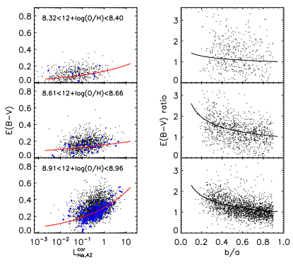
Figure 3 shows that the reddening increases both with increasing $L_{\mathrm{H{\alpha}}}$ and $12+\log\mathrm{(O/H)}$. The intrinsic dust-reddening is clearly correlated with the H$\alpha$ luminosity, with a Spearman rank coefficient $r_{s}=0.59$ (the probability of null hypothesis $P_{\rm null}<10^{-5}$) for our sample of star-forming disc galaxies (Figure 3a). This relation has been known for a long time (e.g. Wang & Heckman 1996; Calzetti et al. 2001; Hopkins et al. 2001; Afonso et al. 2003). The reddening correlates with H$\alpha$ surface brightness as well (not shown in the figure), with $r_{s}=0.51$ ($P_{\rm null}<10^{-5}$). On the other hand, the reddening is also correlated with the gas-phase metallicity indicated by oxygen abundance $12+\log\mathrm{(O/H)}$ ($r_{s}=0.67$, $P_{\rm null}<10^{-5}$, Figure 3b), which has also been known previously (e.g. Heckman et al. 1998; Boissier et al. 2004; Asari et al. 2007). At low metallicity, the reddening increases slowly with [O/H], but at high metallicity, it rises more sharply. The correlation between $E\mathrm{(}B-V)$ and metallcity is the strongest among all of the correlations, therefore we divide our sample into bins of metallicity to investigate the relations of reddening with other parameters (H$\alpha$ luminosity/surface brightness, axial ratio, stellar mass, etc.) at a given metallicity bin in the rest part of this section.

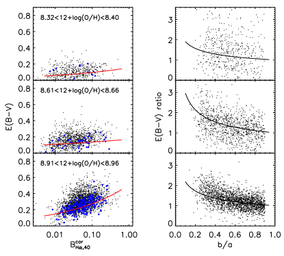
We divide the sample into continuous metallicity bins. The bin is so chosen that a bin-size is no less than 0.05 in $12+\log\mathrm{(O/H)}$, with at least 400 objects in each bin. In order to isolate the inclination-dependence, we check the relation between $E\mathrm{(}B-V)$ and $L_{\mathrm{H{\alpha}}}$ for nearly face-on galaxies, i.e. $(b/a)>0.90$, and then compare it with the rest of the galaxies. Clearly, face-on galaxies have systematically small $E\mathrm{(}B-V)$ values than the others at a given intrinsic $L_{\mathrm{H{\alpha}}}$ (Figure 4, left panel). We fit the relation of reddening with luminosity for these face-on galaxies using a power-law function. For a galaxy, the $E\mathrm{(}B-V)$ ratio is defined as the ratio of $E\mathrm{(}B-V)$ of this galaxy, to the expected $E\mathrm{(}B-V)$ based on its H$\alpha$ luminosity from the best-fitting power-law function for the face-on galaxies. The $E\mathrm{(}B-V)$ ratio is found to correlate with the axial ratio, which can be well fitted by $(b/a)^{\gamma}$. Figure 4 shows $\log L_{\mathrm{H{\alpha}}}$ versus $E\mathrm{(}B-V)$ as well as and the best-fitting curve for the face-on objects on the left panel, and the dependency of the $E\mathrm{(}B-V)$ ratio on the axial ratio b/a on the right panel. These results are only illustrated for three metallicity bins: $12+\log\mathrm{(O/H)}\simeq 8.36$, 8.64 and 8.94 (i.e. $\sim$0.5$Z_{\odot}$, $Z_{\odot}$ and 2$Z_{\odot}$, adopting $[12+\log\mathrm{(O/H)}]_{\odot}=8.66\pm 0.05$, Asplund et al. 2004). The correlation between the $E\mathrm{(}B-V)$ ratio and the axial ratio becomes stronger as the metallcity increases, for example $r_{s}=-0.49$ ($P_{\rm null}<10^{-5}$) for the bottom metallicity bin $12+\log\mathrm{(O/H)}\simeq 8.94$. We fit the data in each bin with a joint function in the form of

$$E\mathrm{(}B-V)\ =pL_{\mathrm{H\alpha},42}^{q}(b/a)^{\gamma},$$ (7)

where $L_{\mathrm{H{\alpha}},42}\equiv L_{\mathrm{H{\alpha}}}/(10^{42}~{}{\rm ergs~{}s^{-1}})$. For each metallicity bin, the fitting parameters are obtained by minimizing $\chi^{2}$ in the fitting implemented by MPFIT, and the results are listed in Table 2. Only uncertainties in $E\mathrm{(}B-V)$ have been considered in the fitting, thus the errors of the fitting parameters are underestimated.

Figure 5: Fitting parameters as a function of metallicity. (a) $p$, (b) $q$ and (c) $\gamma$ are from Equation 7, and (d) $p$, (e) $q$ and (f) $\gamma$ are from Equation 11. Those symbols without error bars indicates the error is smaller than the symbol size. In each panel, the best-fitting function is shown in blue solid line.

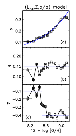
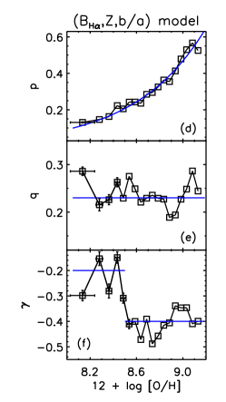
Figure 5 shows $p$, $q$ and $\gamma$ as a function of the metallicity. We can see that $p$ increases with the metallicity, and can be fitted with an exponential function of $12+\log\mathrm{(O/H)}$, i.e. a power-law function of metallicity $Z$, in the form of

$$p\ =0.072^{\pm 0.001}\exp(\frac{x}{0.71^{\pm 0.01}})$$

$$=0.18^{\pm 0.02}\left(\frac{Z}{Z_{\odot}}\right)^{0.61^{\pm 0.01}},$$ (8)

where $x=12+\log\mathrm{(O/H)}\ -8$. The power-law index $q$ varies slightly between 0.08 and 0.17, and the average value is about 0.15. We therefore adopt the parameter $q$ as a constant:

$$\langle q\rangle=0.15.$$ (9)

$|\gamma|$ first increases from about 0.1 with metallicity and then reaches to a constant ($|\gamma|\sim 0.4$) at about $12+\log\mathrm{(O/H)}\simeq 8.5$. We use a step function to fit $\gamma$ as a function of $12+\log\mathrm{(O/H)}$, which is expressed as

$$\gamma\ = -0.1\qquad for\;0.1<x<0.5$$

$$= -0.4\qquad for\;0.5\leq x<1.2$$ . (10)

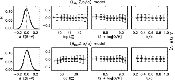
Substitute $p$, $q$ and $\gamma$ into Equation 7, we will get the overall function of luminosity, metallicity and inclination, and we call this ($L_{\mathrm{H{\alpha}}}$, $Z$, b/a) model hereafter. To verify the reliability of our empirical formulae, we define the $E\mathrm{(}B-V)$ residual as $\Delta E\mathrm{(}B-V)\equiv E\mathrm{(}B-V)_{obs}-E\mathrm{(}B-V)_{model}$, and show its distribution in Figure 6 (the first column, upper panel). The $E\mathrm{(}B-V)$ distribution can be well fitted with a Gaussian profile, with width $\sigma=0.068$ mag. If we adopt a more stringent S/N criteria (S/N$>100$) on H$\alpha$ emission, the result will yield a sample of $\sim$5000 star-forming disc galaxies. We repeat the procedure above and find the scatter of $\Delta E\mathrm{(}B-V)$ remains similar, $\sigma=0.066$ mag, indicating that the scatter is independent of H$\alpha$ S/N, in the S/N range we consider (we will discuss in more details and show that our S/N criteria is reasonable in the following Section 4.2). Besides, we find that $\Delta E\mathrm{(}B-V)$ is uncorrelated with the parameters including $L_{\mathrm{H{\alpha}}}$, metallicity or axis ratio (Figure 6, the right three columns), which suggests that the ($L_{\mathrm{H{\alpha}}}$, $Z$, b/a) model considered above reproduces the intrinsic reddening well in the disc galaxies.

Note that at low metallicities the scatter in the relation between $E\mathrm{(}B-V)$ ratio and $b/a$ is larger than that at high metallicities (Figure 5, the right column). The power-law index $\gamma$ is close to zero at low metallcity, i.e. the relationship between $E\mathrm{(}B-V)$ ratio and $b/a$ is almost flat; while $\gamma\sim-0.4$ when the metallicity increases to solar or super-solar value. This suggests that dust reddening is not so sensitive to the axis ratio at low metallicity as at high metallcity. It may be attributed to two possible reasons. One is that the relation at low metallicity might remain as strong as at high metallcity, but the limited dynamic-range of $E\mathrm{(}B-V)$ and the measurement uncertainties prevent us from recovering the relationship. The $E\mathrm{(}B-V)$ dynamic-range is only about 0.2 mag at low metallicity, and increases to 0.8 mag at high metallicity. The other possible reason is that the relation indeed becomes weaker at low metallicity. At present we can not distinguish which one is true, especially when the number of face-on galaxies at low metallicity is limited. If we adopt $\gamma$ to be $-0.4$ for all metallicities, the distribution of $\Delta E\mathrm{(}B-V)$ slightly changes.

Table 2: Coefficients of empirical fits to reddening in a function as in Equation 7, the empirical relation of reddening parameterized by color excess $E\mathrm{(}B-V)$, as a function of $L_{\mathrm{H{\alpha}}}$ and the axial ratio b/a in different metallicity bins.

Metallcity bin	Num	$p$	$q$	$\gamma$	$\chi^{2}_{\nu}$
$12+\log\mathrm{(O/H)}<8.22$	423	$0.104^{\pm 0.003}$	$0.132^{\pm 0.006}$	$-0.196^{\pm 0.027}$	10.75
$8.22<12+\log\mathrm{(O/H)}<8.32$	448	$0.106^{\pm 0.003}$	$0.083^{\pm 0.007}$	$-0.060^{\pm 0.029}$	9.14
$8.32<12+\log\mathrm{(O/H)}<8.40$	515	$0.135^{\pm 0.003}$	$0.159^{\pm 0.007}$	$-0.155^{\pm 0.027}$	7.01
$8.40<12+\log\mathrm{(O/H)}<8.46$	539	$0.139^{\pm 0.003}$	$0.108^{\pm 0.006}$	$-0.054^{\pm 0.023}$	7.41
$8.46<12+\log\mathrm{(O/H)}<8.51$	568	$0.138^{\pm 0.002}$	$0.128^{\pm 0.005}$	$-0.260^{\pm 0.020}$	5.84
$8.51<12+\log\mathrm{(O/H)}<8.56$	733	$0.150^{\pm 0.002}$	$0.138^{\pm 0.005}$	$-0.284^{\pm 0.018}$	6.65
$8.56<12+\log\mathrm{(O/H)}<8.61$	819	$0.162^{\pm 0.002}$	$0.159^{\pm 0.004}$	$-0.292^{\pm 0.014}$	7.26
$8.61<12+\log\mathrm{(O/H)}<8.66$	1088	$0.158^{\pm 0.002}$	$0.141^{\pm 0.004}$	$-0.416^{\pm 0.012}$	6.20
$8.66<12+\log\mathrm{(O/H)}<8.71$	1329	$0.188^{\pm 0.002}$	$0.166^{\pm 0.003}$	$-0.380^{\pm 0.010}$	6.51
$8.71<12+\log\mathrm{(O/H)}<8.76$	1583	$0.195^{\pm 0.001}$	$0.171^{\pm 0.003}$	$-0.418^{\pm 0.009}$	6.09
$8.76<12+\log\mathrm{(O/H)}<8.81$	1917	$0.212^{\pm 0.001}$	$0.165^{\pm 0.003}$	$-0.433^{\pm 0.008}$	7.09
$8.81<12+\log\mathrm{(O/H)}<8.86$	2162	$0.231^{\pm 0.001}$	$0.162^{\pm 0.002}$	$-0.391^{\pm 0.006}$	6.97
$8.86<12+\log\mathrm{(O/H)}<8.91$	2456	$0.241^{\pm 0.001}$	$0.143^{\pm 0.002}$	$-0.438^{\pm 0.006}$	7.02
$8.91<12+\log\mathrm{(O/H)}<8.96$	2551	$0.279^{\pm 0.001}$	$0.152^{\pm 0.002}$	$-0.361^{\pm 0.005}$	8.27
$8.96<12+\log\mathrm{(O/H)}<9.01$	2191	$0.299^{\pm 0.001}$	$0.139^{\pm 0.002}$	$-0.338^{\pm 0.005}$	8.97
$9.01<12+\log\mathrm{(O/H)}<9.06$	1652	$0.315^{\pm 0.001}$	$0.144^{\pm 0.002}$	$-0.368^{\pm 0.006}$	10.64
$9.06<12+\log\mathrm{(O/H)}<9.11$	1052	$0.321^{\pm 0.001}$	$0.154^{\pm 0.002}$	$-0.397^{\pm 0.007}$	13.53
$12+\log\mathrm{(O/H)}>9.11$	590	$0.318^{\pm 0.002}$	$0.166^{\pm 0.003}$	$-0.430^{\pm 0.009}$	11.33

Figure 6: The first column shows the distribution of $E\mathrm{(}B-V)$ residuals in our sample for the two empirical models: the ($L_{\mathrm{H{\alpha}}}$, $Z$, b/a) model and the ($B_{\mathrm{H{\alpha}}}$, $Z$, b/a) model. $\Delta E\mathrm{(}B-V)$ is defined as $\Delta E\mathrm{(}B-V)\equiv E\mathrm{(}B-V)_{obs}-E\mathrm{(}B-V)_{model}$. $N$ is the fraction of the total sample. The best-fitting Gaussian is over-plotted with the centre shown in dotted line for each model. The second to forth column shows $\Delta E\mathrm{(}B-V)$ as a function of $L_{\mathrm{H{\alpha}}}$ or $B_{\mathrm{H{\alpha}}}$ (in units of log ergs s^-1 or ergs s^-1kpc^-2), $12+\log\mathrm{(O/H)}$ and the axial ratio $b/a$, respectively. In each panel, the sample is binned in corresponding parameters, and the median values with 1$\sigma$ dispersions in each bin are shown. The gray dashed line represents $\Delta E\mathrm{(}B-V)=0$.

Figure 7: Left panel: $\log\ B_{\mathrm{H{\alpha}}}$ versus $E\mathrm{(}B-V)$. $B_{\mathrm{H{\alpha}}}$ is in units of ergs s^-1 kpc ^-2. Right panel: The $E\mathrm{(}B-V)$ ratio versus the axial ratio b/a for each metallicity bin. The $E\mathrm{(}B-V)$ ratio is the ratio of $E\mathrm{(}B-V)$ in other galaxies to that deduced from the linear function of $B_{\mathrm{H{\alpha}}}$ for face-on galaxies. The three metallicity bins are 0.5$Z_{\odot}$, $Z_{\odot}$ and 2$Z_{\odot}$, as marked on the left panel. The symbols and the lines represent the same as in Figure 4.

We do similar analysis on how $E\mathrm{(}B-V)$ varies as a function of H$\alpha$ surface brightness and inclination in the metallicity bins, because the H$\alpha$ (SFR) surface density is believed to physically link with the gas surface density, which is closely coupled with dust. Besides, the gas surface density is provided by the current models of galaxy formation. Therefore, the $E\mathrm{(}B-V)$ as a function of H$\alpha$ surface brightness will enable direct application of the empirical relation on the intrinsic reddening in the galaxy evolution models. Figure 7 shows $B_{\mathrm{H{\alpha}}}$ versus $E\mathrm{(}B-V)$ and the best-fitting curve of a power-law function for the face-on objects on the left panel, while the distribution of $E\mathrm{(}B-V)$ ratio against the axial ratio for the three selected metallicity bins on the right panel. In each metallcity bin, we fit the data with a function in the form of

$$E\mathrm{(}B-V)\ =pB_{\mathrm{H\alpha},40}^{q}(b/a)^{\gamma},$$ (11)

where $B_{\mathrm{H{\alpha}},40}\equiv B_{\mathrm{H{\alpha}}}/(10^{40}~{}{\rm ergs~{}s^{-1}kpc^{-2})}$. All the fitting parameters are listed in Table 3. We also fit $p$ with an exponential function of $12+\log\mathrm{(O/H)}$, $q$ with a constant, and $\gamma$ as a step function (Figure 5).

$$p\ =0.092^{\pm 0.001}\exp(\frac{x}{0.61^{\pm 0.01}})$$

$$=0.27^{\pm 0.02}\left(\frac{Z}{Z_{\odot}}\right)^{0.71^{\pm 0.01}},$$ (12)

$$\langle q\rangle=0.23,$$ (13)

and

$$\gamma\ = -0.2\qquad for\;0.1<x<0.5$$

$$= -0.4\qquad for\;0.5\leq x<1.2$$ . (14)

With the model expressed in Equation 11, hereafter ($B_{\mathrm{H{\alpha}}}$, $Z$, b/a) model, we calculate $\Delta E\mathrm{(}B-V)$ and show the distribution in Figure 6. The distribution can be also fitted well with a Gaussian profile, with width $\sigma=0.068$ mag. $\Delta E\mathrm{(}B-V)$ is uncorrelated with the parameters including $B_{\mathrm{H{\alpha}}}$, the metallicity or the axial ratio, which suggests that the ($B_{\mathrm{H{\alpha}}}$, $Z$, b/a) model can reproduce the intrinsic reddening well in the disc galaxies too.

Table 3: Coefficients of empirical fits to reddening in a function as in Equation 11, the empirical relation of $E\mathrm{(}B-V)$ as a function of $B_{\mathrm{H{\alpha}}}$ and the axial ratio b/a in different metallicity bins.

Metallcity bin	Num	$p$	$q$	$\gamma$	$\chi^{2}_{\nu}$
$12+\log\mathrm{(O/H)}<8.22$	423	$0.131^{\pm 0.003}$	$0.286^{\pm 0.009}$	$-0.298^{\pm 0.020}$	9.85
$8.22<12+\log\mathrm{(O/H)}<8.32$	448	$0.147^{\pm 0.006}$	$0.215^{\pm 0.013}$	$-0.154^{\pm 0.027}$	8.78
$8.32<12+\log\mathrm{(O/H)}<8.40$	515	$0.163^{\pm 0.005}$	$0.226^{\pm 0.011}$	$-0.281^{\pm 0.027}$	7.24
$8.40<12+\log\mathrm{(O/H)}<8.46$	539	$0.223^{\pm 0.006}$	$0.263^{\pm 0.010}$	$-0.149^{\pm 0.022}$	6.54
$8.46<12+\log\mathrm{(O/H)}<8.51$	568	$0.205^{\pm 0.005}$	$0.229^{\pm 0.008}$	$-0.309^{\pm 0.020}$	5.34
$8.51<12+\log\mathrm{(O/H)}<8.56$	733	$0.242^{\pm 0.006}$	$0.275^{\pm 0.008}$	$-0.411^{\pm 0.018}$	5.97
$8.56<12+\log\mathrm{(O/H)}<8.61$	819	$0.243^{\pm 0.004}$	$0.249^{\pm 0.006}$	$-0.400^{\pm 0.015}$	6.91
$8.61<12+\log\mathrm{(O/H)}<8.66$	1088	$0.236^{\pm 0.004}$	$0.221^{\pm 0.005}$	$-0.472^{\pm 0.012}$	5.89
$8.66<12+\log\mathrm{(O/H)}<8.71$	1329	$0.285^{\pm 0.004}$	$0.229^{\pm 0.004}$	$-0.391^{\pm 0.010}$	6.31
$8.71<12+\log\mathrm{(O/H)}<8.76$	1583	$0.295^{\pm 0.004}$	$0.236^{\pm 0.004}$	$-0.488^{\pm 0.010}$	5.93
$8.76<12+\log\mathrm{(O/H)}<8.81$	1917	$0.325^{\pm 0.003}$	$0.229^{\pm 0.003}$	$-0.457^{\pm 0.008}$	6.43
$8.81<12+\log\mathrm{(O/H)}<8.86$	2162	$0.363^{\pm 0.003}$	$0.227^{\pm 0.003}$	$-0.415^{\pm 0.007}$	6.58
$8.86<12+\log\mathrm{(O/H)}<8.91$	2456	$0.355^{\pm 0.003}$	$0.189^{\pm 0.003}$	$-0.406^{\pm 0.006}$	6.77
$8.91<12+\log\mathrm{(O/H)}<8.96$	2551	$0.413^{\pm 0.003}$	$0.194^{\pm 0.002}$	$-0.339^{\pm 0.005}$	8.24
$8.96<12+\log\mathrm{(O/H)}<9.01$	2191	$0.479^{\pm 0.003}$	$0.227^{\pm 0.003}$	$-0.347^{\pm 0.005}$	8.42
$9.01<12+\log\mathrm{(O/H)}<9.06$	1652	$0.530^{\pm 0.003}$	$0.248^{\pm 0.003}$	$-0.346^{\pm 0.006}$	9.26
$9.06<12+\log\mathrm{(O/H)}<9.11$	1052	$0.567^{\pm 0.004}$	$0.286^{\pm 0.003}$	$-0.410^{\pm 0.007}$	10.98
$12+\log\mathrm{(O/H)}>9.11$	590	$0.526^{\pm 0.005}$	$0.244^{\pm 0.004}$	$-0.399^{\pm 0.009}$	11.22

In order to investigate the origin of the scatter in the empirical relations, we examine the correlation between $\Delta E\mathrm{(}B-V)$ and other galaxy parameters, such as stellar mass, the 4000 Å break index, EW of Balmer absorption lines, the electron density in H ii region or concentration index. The $\Delta E\mathrm{(}B-V)$ for either ($L_{\mathrm{H{\alpha}}}$, $Z$, b/a) model or ($B_{\mathrm{H{\alpha}}}$, $Z$, b/a) model is not correlated with any of the parameters above, implying that the dust reddening in a disc galaxy is primarily determined by only three physical properties: luminosity (SFR) / surface brightness (SFR surface density), metallicity and disc inclination.

We also attempt another multi-parameter model ($M_{*}$, $Z$, b/a) with similar procedure described above, and find that the scatter of $\Delta E\mathrm{(}B-V)$ is 0.072 mag, which is slightly larger than the two models above (Equation 7 and 11). However, $\Delta E\mathrm{(}B-V)$ for this model is still weakly correlated with $L_{\mathrm{H{\alpha}}}$ ($r_{s}=0.15$, $P_{\rm null}<10^{-5}$). This suggests that ($L_{\mathrm{H{\alpha}}}$ or SFR, $Z$) combination works better than ($M_{*}$, $Z$) combination. Physically, at a given metallicity, the amount of dust is proportional to the amount of cold gas, which is closely correlated with SFR.

4.1 Comparison with previous work

We compare our models with previous empirical relations. Garn & Best (2010) investigate the dependency of dust extinction at H$\alpha$ on SFR, metallicity and stellar mass respectively, in star-forming galaxies based on SDSS database. They conclude that the stellar mass is the most fundamental parameter in determining the dust extinction in the local Universe, and their relation between stellar mass and dust extinction seems to hold up to redshift of 1.5 (Sobral et al. 2011). They utilize different models to fit the extinction $A_{\mathrm{H{\alpha}}}$, with each model taking into consideration one of the three parameters: SFR, $M_{*}$ and metallicity. They find that the $M_{*}$ model gives the best fit, with the minimum of scatter (0.28 mag) in the extinction residual $\Delta A_{\mathrm{H{\alpha}}}\equiv A_{\mathrm{H{\alpha}}}^{obs}-A_{\mathrm{H{\alpha}}}^{model}$, less than the scatter for SFR model and metallicity model, both of which are 0.33 mag. When calculating the $A_{\mathrm{H{\alpha}}}$, they adopt the Calzetti et al. (2000) dust attenuation-curve. We repeat their analysis for our selected sample of disc galaxies and compare the scatter of $\Delta A_{\mathrm{H{\alpha}}}$ among different models. In each model a low-order (third order) polynomial is adopted to fit the extinction, and the distribution of $\Delta A_{\mathrm{H{\alpha}}}$ is well fitted by a Gaussian, with widths $\sigma=$0.27, 0.28 and 0.28 mag for the $M_{*}$, $L_{\mathrm{H{\alpha}}}$ (SFR) and metallicity model respectively. Higher order polynomial fits will not decrease the scatter. We check the scatter of $\Delta A_{\mathrm{H{\alpha}}}$ for our ($L_{\mathrm{H{\alpha}}}$, $Z$, b/a) or ($B_{\mathrm{H{\alpha}}}$, $Z$, b/a) model assuming Calzetti’s attenuation law, and the Gaussian width is only $\sigma=0.22$ mag (corresponding to $\sigma=0.065$ mag for the $\Delta E\mathrm{(}B-V)$ distribution). We also check for the ($M_{*}$, $Z$, b/a) model, and find that the scatter of $\Delta A_{\mathrm{H{\alpha}}}$ is 0.24 mag, which is better than the single-parameter models, but worse than the other two multi-parameter models.

Our empirical relations predict dust reddening better than the single-parameter models, probably because we include disc inclination in the analysis. In order to investigate what dominates the relationships of the variables, we apply principle component analysis on the physical variables. The derived principle components (PCs) are linear combinations of the variables, and represent for the directions of maximum variance in the data. For H$\alpha$ luminosity and surface brightness, $E\mathrm{(}B-V)$, $M_{*}$ and metallicity, the quantities are normalized to zero mean and standard deviation of unity, while for the axial ratio original value is used. We test with different subsets of variables adopted in each multi-parameter model as well as all of the variables, and find similar results. Take the case of ($L_{\mathrm{H{\alpha}}}$, $Z$, b/a) model for example, the first two PCs contribute to about 80 percent of the total variance. In PC1, the variables $L_{\mathrm{H{\alpha}}}$, $Z$ and $E\mathrm{(}B-V)$ weight almost equivalently. This is consistent with what Garn & Best (2010) found. But in PC2 the axial ratio weights the most (-0.98) and $E\mathrm{(}B-V)$ weights the second (0.30). The result is consistent with what we previously found. Although the axial ratio only weakly correlated with $E\mathrm{(}B-V)$ ($r_{s}=-0.13$, $P_{\rm null}<10^{-5}$), after removing the $E\mathrm{(}B-V)$ dependence on H$\alpha$ luminosity and metallicity, the negative correlation between $b/a$ and $E\mathrm{(}B-V)$ emerges.

4.2 Error analysis

We have shown that the global reddening of the emission lines from a disc galaxy can be reasonably determined by its H$\alpha$ luminosity or surface brightness, gas metallicity and disc inclination. The $1\sigma$ scatter of $\Delta E\mathrm{(}B-V)$ is about 0.07 mag, which is contributed by several sources, including the measurement uncertainty in the Balmer decrement, the error in the metallicity, the uncertainties in other variables and the intrinsic scatter in the relation. We will discuss the uncertainties in the following.

Let us take a review of the uncertainties in the physical quantities. The formal error for $L_{\mathrm{H{\alpha}}}$ measurement is 0.04 dex, and for $B_{\mathrm{H{\alpha}}}$ is 0.05 dex. As discussed in Section 3.2, the uncertainty induced by aperture-correction and attenuation-correction is less than 0.12 dex. The typical error of $b/a$ is 0.02. The uncertainty in metallicity calibration dominates the uncertainty of metallicity, estimated to be $\sim 0.15$ dex. We use Monte Carlo simulation to estimate the error of $E\mathrm{(}B-V)$ for Equation 7 and 11 taking the uncertainties for the best-fit parameters and the measurement errors for the physical variables. The errors of $E\mathrm{(}B-V)$ predicted by Equation 7 and 11 are both about 0.056 mag. If taking the uncertainty in aperture-correction and attenuation-correction (0.12 dex at most) into account in $L_{\mathrm{H{\alpha}}}$ and $B_{\mathrm{H{\alpha}}}$ error, the simulated $E\mathrm{(}B-V)$ errors slightly changes to 0.058 mag. Remember that the measurement error of $E\mathrm{(}B-V)$ is 0.03 mag, the scatter of $\Delta E\mathrm{(}B-V)$ (0.07 mag) can be almost explained by the uncertainties of the physical quantities. Considering all these uncertainties, $E\mathrm{(}B-V)$ predicted from the empirical relations are quite consistent with the observed values.

From Figure 6 we can see that the $\Delta E\mathrm{(}B-V)$ distribution can be well described by a Gaussian profile, indicative of a random distribution. However, the intrinsic scatter of the empirical relation is still unclear, because of the large uncertainty in the metallicity calibration. Therefore, to estimate the intrinsic scatter of the relation, it will be of help to decrease the uncertainty in the metallicity calibration and obtain the metallicity more precisely. One may find there is slight excess over the positive tail of the gaussian distribution. We examine the objects (about one percent of the whole sample) with $\Delta E\mathrm{(}B-V)>0.2$, i.e. the observed $E\mathrm{(}B-V)$ is under-estimated with our empirical models by 0.2 mag, and find that these objects are prone to large Balmer decrement, low H$\beta$ S/N and low H$\beta$ EW.

As previously mentioned, we require S/N$>20$ for H$\alpha$, and S/N$>10$ for H$\beta$ and [O iii] when selecting our sample in Section 2. The S/N criteria for H$\alpha$ will exclude some galaxies with low SFR and low H$\alpha$ EW. Thus the number of galaxies with low H$\alpha$ luminosity and low SFR will be reduced. In fact, when the criteria S/N$>10$ is applied for H$\beta$, most of the remaining sample ($\sim$99.9 percent) will have H$\alpha$ S/N$>20$. In order to investigate whether the H$\beta$ and [O iii] S/N criteria bias our results, we attempt a looser S/N($>5$) criteria for both lines, and the sample is expanded by 50 percent to have 34815 galaxies. Then we fit the data with both the ($L_{\mathrm{H{\alpha}}}$, $Z$, b/a) model and ($B_{\mathrm{H{\alpha}}}$, $Z$, b/a) model. The results show that the fit parameters are quite similar as those we have obtained in Section 4, but the scatter in $\Delta E\mathrm{(}B-V)$ increases to about 0.08 mag. Note that 10 percent uncertainty in H$\alpha$/H$\beta$ will result in an uncertainty of 0.086 mag in $E\mathrm{(}B-V)$, which explains the increased scatter. Thus including the low S/N objects merely introduces more scatter in the relation.

5 A TOY MODEL ON DUST EXTINCTION TO H ii REGIONS IN A DISC GALAXY

Two different sources contribute to the extinction for H ii regions: dust associated with the individual H ii region and diffuse foreground dust in the galaxy. Let us first consider the dust in the precursor molecular clouds (MC). The intrinsic extinction in individual H ii region depends on the relative distribution of young massive stars, gas and dust in the star-formation regions, which are also closely related to the age and size of the precursor MC, as well as the stochastic formation of high mass stars for a given initial mass function. An H ii region is embedded in the cold gas/dust envelope before the cold gas/dust is blown away. The time scale for such a process is expected to depend on the size and density of the precursor cloud: longer for more massive and dense H ii region. Panuzzo et al. (2003) discussed the attenuation to the H$\alpha$ emission line for different evaporating time scale, in comparison with the lifetime of massive stars that produce the ionizing continuum. They simply adopt a central ionizing star in a spherical cloud, which corresponds to the maximum attenuation case. If the time scale is short enough, most H ii regions are produced outside of the MC, and the main attenuation is due to foreground dust. In the case of long evaporation time, an H ii region is buried in the MC during most of their life time and the extinction associated with the H ii region will be important. In a galaxy, all these cases are likely present. Furthermore, the young ionizing stars are not necessarily forming in the cloud centre. These complications make any prediction of the reddening in an individual cloud rather difficult.

However, as far as a large number of H ii regions are concerned, the statistical behavior may be quite well defined. The H$\alpha$ luminosity function of H ii regions in spiral galaxies can be described by double power-law functions, with a flatter power-law below the break luminosity of 38.6 (in units of ergs s^-1, logarithmic), and a steeper one above it (e.g. Kennicutt et al. 1989; Bradley et al. 2006). In our sample, most galaxies have H$\alpha$ luminosities above 40 (in units of ergs s^-1, logarithmic) with a median of 41.5, and the maximum is 43.3. Therefore, a galaxy consists of numerous (order of hundreds to millions of) H ii regions. The H ii regions follow certain distributions of ages and initial masses, determined by the star-formation processes, because the star-formation time in a galaxy is likely much longer than the lifetime of an individual H ii region, i.e. the life time of OB stars. If these distributions are the same for each galaxy and there are a large number of H ii regions, one may expect that the average extinction within H ii regions should be similar in each galaxy. In this respect, it is not expected that the dust reddening depends on the H$\alpha$ luminosity or the inclination of the disc. In contrast, for example, if the MC mass function and stellar IMF depend on the global properties of the galaxies, such as the gas surface density, then one may expect that the average extinction is correlated with the global properties. However, this is poorly known so far.

Next, we consider the extinction due to diffuse interstellar dust in a galaxy. It is expected that this extinction depends on the gas surface density, inclination, metallicity of the interstellar medium and size of the galaxy. To simplify the model, we will adopt smooth distributions for the dust, gas and star-formation regions with the following assumptions:

(1)

dust-to-gas density ratio is proportional to the gas metallicity (Issa et al. 1990), i.e., gas and dust are coupled:

$$\rho_{\mathrm{d}}\propto\rho_{\mathrm{g}}\times Z,$$ (15)

where $\rho_{\mathrm{d}}$ and $\rho_{\mathrm{g}}$ are dust density and gas density, respectively;

(2)

both gas and dust distributions in the vertical ($z$) and radial ($R$) direction can be described by an exponential law (e.g. de Jong 1996; Thomas et al. 2004; Misiriotis et al. 2006), i.e.,

$$\rho_{\mathrm{g}}=\rho_{\mathrm{g}}(0)\exp(-z/h_{\mathrm{g}})\exp(-R/R_{\mathrm{g}}),$$ (16)

where $\rho_{\mathrm{g}}(0)$ is the gas density at $z=0$ and $R=0$, $h_{\mathrm{g}}$ and $R_{\mathrm{g}}$ are the characteristic lengths in the vertical and radial directions for gas distribution. But the dust distribution may have different length scales due to radial metallicity gradient:

$$\rho_{\mathrm{d}}=\rho_{\mathrm{d}}(0)\exp(-z/h_{\mathrm{d}})\exp(-R/R_{\mathrm{d}}),$$ (17)

where $\rho_{\mathrm{d}}(0)$ is the dust density at $z=0$ and $R=0$, $h_{\mathrm{d}}$ and $R_{\mathrm{d}}$ are the characteristic lengths in the vertical and radial directions for dust distribution;

(3)

the H ii distribution is also exponential in both radial and vertical direction, but with different characteristic lengths (e.g. de Jong 1996):

$$\rho_{\mathrm{H\alpha}}=\rho_{\mathrm{H\alpha}}(0)\exp(-z/h_{\mathrm{H\alpha}})\exp(-R/R_{\mathrm{H\alpha}}).$$ (18)

By integrating $\rho_{\mathrm{H\alpha}}$ over $z$ direction, we yield a surface density of H$\alpha$, $\Sigma_{\mathrm{H\alpha}}$. Specifically, the H$\alpha$ surface density at $R=0$ is

$$\Sigma_{\mathrm{H\alpha,0}} = \int_{0}^{\infty}\rho_{\mathrm{H\alpha}}(0)\exp(-z/h_{\mathrm{H\alpha}})dz+\int_{-\infty}^{0}\rho_{\mathrm{H\alpha}}(0)\exp(z/h_{\mathrm{H\alpha}})dz$$ (19)

$$= 2\rho_{\mathrm{H\alpha}}(0)h_{\mathrm{H\alpha}}$$

The gas disc is rather thin in general. As a result, dust attenuation can be modeled as plane-parallel except at extremely high inclinations. Young stars are formed in dense molecular cores, which might be distributed in a plane thinner than the gas disc. For a plane-parallel model, the optical depth is expressed as

$$\tau\ =\rho_{\mathrm{d}}k_{\nu}z/\cos i,$$ (20)

where $k_{\nu}$ is the opacity coefficient, and $i$ is the inclination angle, and $i=0^{\degr}$ represents the line of sight perpendicular to the galaxy disc, while $i=90^{\degr}$ represents the line of sight parallel to the galaxy disc. The optical depth to H$\alpha$ emission from the middle plane of the disc to the upper disc surface at $R=0$ is defined as

$$\tau_{\mathrm{H\alpha,0}}=\int_{0}^{\infty}\rho_{\mathrm{d}}(0)k_{\nu}\exp(-h/h_{\mathrm{d}})dh=\rho_{\mathrm{d}}(0)k_{\nu}h_{\mathrm{d}}.$$ (21)

It is symmetric between the middle plane to the upper and lower disc surface, thus the overall optical depth through the whole disk vertically at $R=0$ should be $2\tau_{\mathrm{H\alpha,0}}$. Then we consider the optical depth from the point at $z$($>0$) on the vertical axis ($R=0$) to the upper surface of the disc is

$$\tau_{1}(z)=\int_{z}^{\infty}\rho_{\mathrm{d}}(0)k_{\nu}\exp(-h/h_{\mathrm{d}})dh=\tau_{\mathrm{H\alpha,0}}\exp(-z/h_{\mathrm{d}}),$$ (22)

and the optical depth from that point to the lower disc surface can be expressed as

$$\tau_{2}(z)=2\tau_{\mathrm{H\alpha,0}}-\tau_{1}(z).$$ (23)

Light from the H ii regions at the position ($z$, $R$) needs to travel through the disc, from both upper and lower sides. With these descriptions, we can calculate the H$\alpha$ luminosity, H$\alpha$ surface brightness and average attenuation at H$\alpha$ and H$\beta$ by integrating the radiation transfer function over both vertical and radial directions within the disc. Then the H$\alpha$ luminosity is

$$L_{\mathrm{H{\alpha}}}\ =\int_{0}^{2}\pi d\theta\int_{0}^{R_{H\alpha,max}}RdR\int_{0}^{\infty}\rho_{\mathrm{H\alpha}}$$

$$\{\exp[-\frac{\tau_{1}(z)}{\cos i}\exp(-R/R_{\mathrm{d}})]+exp[-\frac{\tau_{2}(z)}{\cos i}\exp(-R/R_{\mathrm{d}})]\}.$$ (24)

Substitue Equation 18, 22, 23, $y=\exp(-z/h_{\mathrm{H\alpha}})$ and $a=R/R_{\mathrm{H\alpha}}$ into Equation 24, then we get

$$L_{\mathrm{H{\alpha}}}\ = \pi R^{2}_{\mathrm{H\alpha}}\Sigma_{\mathrm{H\alpha,0}}\int_{0}^{1}dy\int_{0}^{\xi}ada\exp(-a)\{$$ (25)

$$\exp[-\frac{\tau_{\mathrm{H\alpha,0}}}{\cos i}\exp(-a/\eta)y^{1/\kappa}]+$$

$$\hskip 20.00003pt\exp[-\frac{\tau_{\mathrm{H\alpha,0}}}{\cos i}\exp(-a/\eta)(2-y^{1/\kappa})]\},$$

where $\xi\equiv R_{\mathrm{H\alpha,max}}/R_{\mathrm{H\alpha}}$ is set by the threshold surface density of star formation $R_{\mathrm{H\alpha,max}}\equiv R_{\mathrm{g}}\ln(\Sigma_{\mathrm{g,0}}/\Sigma_{\mathrm{th}})$; and the threshold gas surface density is adopted as $\Sigma_{\mathrm{th}}\simeq 5M_{\sun}$ pc^-2(Martin & Kennicutt 2001); $\Sigma_{\mathrm{g,0}}$ is the surface density of gas at $R=0$; $\eta=R_{\mathrm{d}}/R_{\mathrm{H\alpha}}$ and $\kappa=h_{\mathrm{d}}/h_{\mathrm{H\alpha}}$. In order to reduce the number of free parameters ($\Sigma_{H\alpha,0}$, $\tau_{\mathrm{H\alpha,0}}$, $\cos i$, $\xi$, $\eta$ and $\kappa$), we use the empirical relation between the SFR surface density $\Sigma_{\mathrm{SFR}}$ and gas surface density $\Sigma_{\mathrm{g}}$ (known as Schmidt-Kennicutt law; Kennicutt et al. 1998):

$$\Sigma_{\mathrm{SFR}}\ (M_{\sun}\mathrm{yr^{-1}kpc^{-2}})$$

$$=(2.5\pm 0.7) \times 10^{-4}\left(\frac{\Sigma_{\mathrm{g}}}{M_{\sun}\mathrm{pc}^{-2}}\right)^{1.4\pm 0.15}.$$ (26)

Reminding that the gas and H ii distributions are both exponential, we will get $R_{\mathrm{g}}=1.4R_{\mathrm{H\alpha}}$. With above relations and the conversion between $L_{\mathrm{H{\alpha}}}$ and SFR (Equation 3), we can write:

$$\xi=\ln\frac{\Sigma_{\mathrm{H\alpha,0}}}{4.4\times 10^{38}~{}\mathrm{ergs~{}s^{-1}~{}kpc}^{-2}}.$$ (27)

Assuming the dust-to-gas ratio to be the same as in the Galactic disc, i.e., $E\mathrm{(}B-V)\ =1.7\times 10^{-22}N_{\mathrm{H}}(Z/Z_{\odot})$ (Bohlin 1978) and a Galactic extinction curve (Fitzpatrick 1999), we obtain the effective optical depth to H$\alpha$ through the disc perpendicularly as

$$\tau_{\mathrm{H\alpha,0}}=0.5\left(\frac{\Sigma_{\mathrm{H\alpha,0}}}{3.3\times 10^{39}~{}{\mathrm{ergs~{}s^{-1}}~{}\mathrm{kpc}^{-2}}}\right)^{0.714}\frac{Z}{Z_{\odot}}.$$ (28)

Once we have $\tau$, it is straightforward to calculate the extinction at H$\alpha$ using Equation 25 as following

$$A_{\mathrm{H{\alpha}}}\ = -2.5\log\left(\frac{L_{\mathrm{H{\alpha}},\tau}}{L_{\mathrm{H{\alpha}},\tau=0}}\right)\$$ (29)

$$= \int_{0}^{1}dy\int_{0}^{\xi}ada\exp(-a)\{\exp[-\frac{\tau_{\mathrm{H\alpha,0}}}{\cos i}\exp(-a/\eta)y^{1/\kappa}]+$$

$$\hskip 20.00003pt\exp[-\frac{\tau_{\mathrm{H\alpha,0}}}{\cos i}\exp(-a/\eta)(2-y^{1/\kappa})]\}/$$

$$\hskip 30.00005pt2[1-\exp(-\xi)-\xi\exp(-\xi)],$$

Similarly, replacing $\tau_{\mathrm{H\alpha,0}}$ with $\tau_{\mathrm{H\beta,0}}$, one obtains the extinction at H$\beta$. Thus H$\alpha$/H$\beta$ ratio can be calculated, and then $L_{\mathrm{H{\alpha}}}$ can be corrected with the extinction estimated from the Balmer decrement, as the extinction correction we make to the observed $L_{\mathrm{H{\alpha}}}$.

In order to examine if such a model can reproduce the observed correlations, we compute the average surface brightness $B_{\mathrm{H{\alpha}}}$ and color excess $E\mathrm{(}B-V)$ estimated by H$\alpha$/H$\beta$ from the model based on the following parameters: $\Sigma_{H\alpha,0}$, $Z$, $\cos i$, $\eta$ and $\kappa$. To facilitate comparison with observation, we obtain $B_{\mathrm{H{\alpha}}}$ following the same method used for observation (Equation 6) by dividing the attenuation-corrected $L_{\mathrm{H{\alpha}}}$ with the surface within the half-light radius, defined as the radius within which the H$\alpha$ luminosity is half of the total $L_{\mathrm{H{\alpha}}}$. The $E\mathrm{(}B-V)$ is calculated from $A_{\mathrm{H{\alpha}}}$ and $A_{\mathrm{H{\beta}}}$ assuming Fitzpatrick’s extinction curve. We first fix $\eta$ to be 1. Since increasing metallicity and inclination both cause an increase in extinction, these two factors are coupled in the model. Therefore, we incorporate them into one parameter $Zi\equiv Z/\cos i$. We compute the models for a grid of parameters with $38.5<\log\Sigma_{H\alpha,0}<42.0$, $Zi=0.5,\ 1.5,\ 2.5,\ 3.5,\ 4.5$, $\kappa=0.5,\ 1,\ 2,\ 5$.

Figure 8: Average surface brightness $B_{\mathrm{H{\alpha}}}$ (ergs s^-1 kpc^-2, corrected for extinction) versus $E\mathrm{(}B-V)$, with the relative characteristic lengths of dust to H ii regions distribution in radial direction $\eta=1$ (left panel) and $\eta=1.2$ (right panel). Observation sample with $Z/\cos i$, marked as $Zi$ for short, in bins of $0.5\pm 0.1$, $1.5\pm 0.1$, $2.5\pm 0.1$, $3.5\pm 0.1$, and $4.5\pm 0.1$ are shown. Dotted (blue) line represents for the relative characteristic lengths of dust to H ii regions distribution in vertical direction $\kappa=0.5$, solid (red) line for $\kappa=1$, dashed (magenta) line for $\kappa=2$, and dash-dotted (green) line for $\kappa=5$.

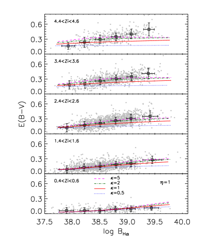
The models are over-plotted on the observation sample on the $B_{\mathrm{H{\alpha}}}$ versus $E\mathrm{(}B-V)$ plane (Figure 8). For clarity, we only show the observation sample in five bins of $Zi$ with a bin-width of 0.2, and on each panel the subsample is binned in $B_{\mathrm{H{\alpha}}}$ and shown in squares with error bars. We can see the observation trend on each panel, that $E\mathrm{(}B-V)$ increases as $B_{\mathrm{H{\alpha}}}$ increases. The model curves are calculated with the corresponding value of median $Zi$ for each subsample. On each panel, $E\mathrm{(}B-V)$ gets larger when $\kappa$ increases, and each curve with constant $\kappa$ first increases and then becomes flat as $B_{\mathrm{H{\alpha}}}$ increases. At small $\kappa$, i.e. the dust layer is much thinner than the stellar disc, $E\mathrm{(}B-V)$ saturates at a small value because the Balmer-line emission from the disc of larger height tends to dominate, resulting in a small $E\mathrm{(}B-V)$, while at large $\kappa$ more Balmer-line emission comes from the inner region close to the midplane of the disc, thus tend to have a large $E\mathrm{(}B-V)$. The saturation is due to the fact that the observed light from outside weights more as the optical depth increases.

Generally the $\kappa=1$ model reproduces the observed correlations at low $Zi$. However, as $Zi$ increases, the constant $\kappa$ model is lower than the observation trend at the high-end of $B_{\mathrm{H{\alpha}}}$. At medium $Zi$ (1.5$\sim$2.5), the observation can be better presented by the model with larger $\kappa$ (e.g. $\kappa\geq 2$). This could be explained by the vertical expansion of dust distribution in the disc while higher surface brightness indicates intenser star-formation activity. The dust may be driven away from the midplane of the disc by radiation pressure or the stellar winds, thus the dust layer become thicker than that for low $B_{\mathrm{H{\alpha}}}$. But $E\mathrm{(}B-V)$ saturates at about 0.3 mag when $\kappa\geq 2$, which means that the effective optical depth saturates when the height of dust layer gets to twice height of H ii regions. Another possible explanation is that the Kennicutt-Schimidt law we adopt in the model is an averaged star formation law that linked between the surface density of gas and star formation as the form of $\Sigma_{\mathrm{SFR}}\propto\Sigma_{\mathrm{g}}^{N}$. Leroy et al. (2008) suggested that the star formation law may vary as a function of local conditions at different galactocentric radius, including metallicity and the dominated gas content (H i or H₂). The SF law has smaller $N$ value at higher $\Sigma_{\mathrm{SFR}}$ in the inner region of a galaxy (e.g. Bigiel et al. 2008, their Figure 11), thus large dust reddening in the inner region dominates the observed $E\mathrm{(}B-V)$. As a result, the dust reddening is higher than that the present model predicts.

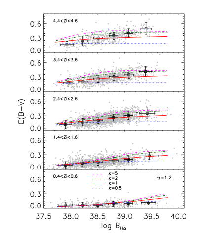
In the model above, we assume $\eta=1$, i.e. the dust and H ii region has the same characteristic scale in the radial distribution, but the gas/dust may distribute at larger radii than the star-forming regions (e.g. Bigiel et al. 2008). Thus we also consider $\eta=1.2$, and find that the observation with large $Zi$ can be well explained by model with $\kappa=1$ at low $B_{\mathrm{H{\alpha}}}$ and $\kappa\geq 2$ at high $B_{\mathrm{H{\alpha}}}$. It is possible because in a spiral galaxy centre, where the metallicity is higher than outside, we are observing the star-formation dominated centre, and the gas (or dust) distribution is more extended.

In this simple toy model, the optical depth $\tau_{H\alpha}$ is assumed to be proportional to the metallicity $Z$. It comes from the assumption that $\rho_{\mathrm{d}}\propto\rho_{\mathrm{g}}\times Z$. However, there is evidence that this assumption may be not the case in practice. Boissier et al. (2004) studied six nearby late-type galaxies in FIR and UV images, and find that the dust-to-gas ratio is proportional to $(Z/Z_{\odot})^{0.88}$, which was flatter than the linear correlation we adopted above. This suggests that the dust-to-gas ratio may not evolve linearly with $Z$. In addition, we assume in the model that the disc height is very thin, i.e. the disc height is quite small compared to the disc radius, thus the radial gradient in gas density can be neglected when calculating $\tau_{H\alpha}$. Under that assumption, the effect of inclination on optical depth can be expressed as $(\cos i)^{-1}$. However, in practice, the disc may not have a uniform height, for instance, it may be thicker in the centre and thinner at large radii, or the presence of bulge in the disc centre. Also, the distribution of dust and star-formation regions may be not smooth, for example when the spiral arms are present in the disc galaxy. In those cases, the inclination factor might be flatter than $(\cos i)^{-1}$. Accounting for these realistic effects, we adjust $Z/Z_{\odot}$ to $(Z/Z_{\odot})^{\alpha}$ in Equation 28 and $(\cos i)^{-1}$ to $(\cos i)^{-\alpha}$ in Equation 25 and 29, then test several values for the power-law index. It turns out that with $\alpha=0.7$ the simple model reproduces the observation trend well (Figure 9). When $Zi$ is low, the model of constant $\kappa$ (0.5 or 1) reproduces the observation trend well. While $Zi$ is higher, the observation can be reproduced with the model of $\kappa\geq 2$.

Figure 9: Same figure as Figure 8, except that the model is calculated with Equation 28 and 29, but adjusting $Z/Z_{\odot}$ to $(Z/Z_{\odot})^{0.7}$, and $\cos i$ to $(\cos i)^{0.7}$.

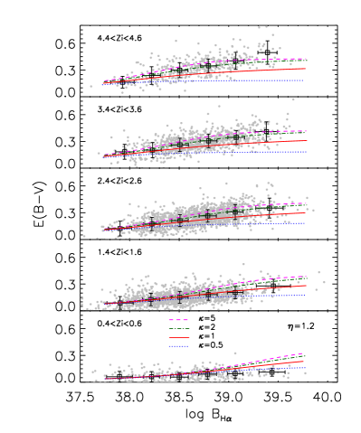
To summarize, the simple toy models reproduce the observed trends between dust reddening and H$\alpha$ surface brightness, that reddening increases with $B_{\mathrm{H{\alpha}}}$. The comparisons between observation and the toy models indicate that, the relative distribution of H ii regions to gas/dust both in vertical and radial direction of the galaxy disc, may vary in different environment of star-formation activity levels or metallicities. The dust might be distributed further beyond the H ii regions when the star formation activity is intenser, or the dust is distributed in a thicker disc ($\kappa\geq 1$) than the H ii regions when the metallicity gets higher. In addition, our results imply that dust-to-gas density ratio may be not proportional to the metallicity $Z$, but to a power-law of $Z$, $Z^{\alpha}$ with $\alpha\sim 0.7$.

6 CONCLUSIONS AND IMPLICATIONS

We present the empirical formulae of intrinsic reddening as a function of intrinsic H$\alpha$ luminosity or surface brightness, metallicity and disc inclination (Equation 7, 11 and Table 2 and 3) for a large sample of $\sim$22 000 well-defined star-forming disc galaxies selected from the SDSS. With the empirical formulae, the reddening parameterized by $E\mathrm{(}B-V)$ could be predicted within 1$\sigma$ uncertainty of 0.07 mag. The $\Delta E\mathrm{(}B-V)$, defined as the observed reddening estimated from the Balmer decrement minus predicted value, does not correlate with the three parameters used in the formulae. We also find that $\Delta E\mathrm{(}B-V)$ is independent of the stellar mass, 4000 Å break strength or electron density within the galaxy.

The observed trend between the dust reddening and H$\alpha$ surface brightness could be reproduced by a plane-parallel slab toy model, in which the dust is scaled with gas, and all the distributions of the dust, gas and star-formation regions are smooth and follow exponential laws in the disc. We find from the comparisons of the models to the observation, the relative vertical scale of dust distribution to H ii regions distribution may vary with H$\alpha$ surface brightness or metallicity. The higher intensity of star formation could drive the dust to distribute in a thicker layer, or the dust disc is thicker than the disc of the H ii regions when the metallicity is higher. However, the real galaxies may be not fully described by this simple toy model. For example, when the spiral arms are present, or the SF regions are clumpy, the assumptions of smooth distributions will be improper. In addition, our result implies a different scaling law of dust-to-gas ratio as a function of metallicity $Z$ from the linearly relation (Equation 15). Our empirical relations, which suggest dust reddening is partially dependent on metallicity ($\propto Z^{0.6\sim 0.7}$), can be an observational constraints on the output of radiative-transfer model calculations, and hence provides constraints on the assumed dust-to-gas ratio in the model.

Since metallicity-dependence has been introduced, we believe that our empirical formulae should be applicable to the early evolutionary stage of a galaxy, when the gas metallicity might be low. In the starburst galaxies at high redshift, dust surrounding star-forming region has been proven to be prone to sub-milimeter and far-infrared observations. But most of those galaxies are relatively dim in optical, implying severe extinction and reddening to these galaxies. The observed galaxies at high redshifts are affected by reddening, in the way that the galaxies with heavy attenuation and reddening may escape from the detection. The importance of the reddening correction depends on the wavelength band that is used. For example, UV continuum luminosity is usually used to infer SFR in high-redshift galaxies. It is very sensitive to the attenuation/reddening. Calzetti et al. (2000) find that the extinction to emission lines and to stellar continuum in optical band are different, and the continuum reddening is only about 40 percent of that for emission lines. However, the extinction to UV continuum is likely similar to the H ii region because UV continuum is also emitted by young hot stars, which are likely surrounded by H ii regions. As a result, our results may be used to estimate the reddening for these high-redshift galaxies with caution, that the metallicity should be well-calibrated and be within the range covered by our sample. Following Equation 7 and the discussions in Section 4, SFR in luminous star formation or high metallicity galaxies might have been under-estimated (e.g. Heckman et al. 1998; Hopkins et al. 2001; Panuzzo et al. 2007), or those galaxies are even completely lost in optical surveys.

The quantitative relationship of reddening with the metallicity, luminosity or surface brightness, and the inclination for disc galaxies can also be incorporated into the current semi-analytic models of galaxy formation and evolution (e.g. Croton et al. 2006; De Lucia et al. 2004; Kang et al. 2005). In those models, a simple chemical enrichment scheme has been included, and the metal abundance has been actually predicted. With the known metallicity and the star formation rate (intrinsic luminosity) provided by the models, the reddening can be estimated accurately with our formulae, and then used to shape the spectral energy distribution and predict the emerging luminosity more realistically.

References

- Adelman-McCarthy et al. (2007) Adelman-McCarthy, J. K., et al. 2007, ApJS, 172, 634
- Afonso et al. (2003) Afonso, J., Hopkins, A., Mobasher, B., & Almeida, C. 2003, ApJ, 597, 269
- Allende Prieto et al. (2001) Allende Prieto, C., Lambert, D. L., & Asplund, M. 2001, ApJ, 556, L63
- Alonso-Herrero et al. (2006) Alonso-Herrero, A., Rieke, G. H., Rieke, M. J., Colina, L., Pérez-González, P. G., & Ryder, S. D. 2006, ApJ, 650, 835
- Asari et al. (2007) Asari, N. V., Cid Fernandes, R., Stasińska, G., Torres-Papaqui, J. P., Mateus, A., Sodré, L., Schoenell, W., & Gomes, J. M. 2007, MNRAS, 381, 263
- Asplund et al. (2004) Asplund, M., Grevesse, N., Sauval, A. J., Allende Prieto, C., & Kiselman, D. 2004, A&A, 417, 751
- Baldwin et al. (1981) Baldwin, J. A., Phillips, M. M., & Terlevich, R. 1981, PASP, 93, 5
- Balogh et al. (1999) Balogh, M. L., Morris, S., Yee, H., Carlberg, R., & Ellingson, E. 1999, ApJ, 527, 54
- Bianchi & Efremova (2006) Bianchi, L., & Efremova, B. V. 2006, AJ, 132, 378
- Bigiel et al. (2008) Bigiel, F., Leroy, A., Walter, F., Brinks, E., de Blok, W. J. G., Madore, B., & Thornley, M. D. 2008, AJ, 136, 2846
- Blanton et al. (2001) Blanton, M. R., et al. 2001, AJ, 121, 2358
- Blanton & Roweis (2007) Blanton, M. R., & Roweis, S. 2007, AJ, 133, 734
- Boissier et al. (2004) Boissier, S., Boselli, A., Buat, V., Donas, J., & Milliard, B. 2004, A&A, 424, 465
- Bradley et al. (2006) Bradley, T. R., Knapen, J. H., Beckman, J. E., & Folkes, S. L. 2006, A&A, 459, L13
- Brinchmann et al. (2004) Brinchmann, J., Charlot, S., White, S. D. M., Tremonti, C., Kauffmann, G., Heckman, T., & Brinkmann, J. 2004, MNRAS, 351, 1151
- Bruzual (1983) Bruzual, A. G. 1983, ApJ, 273, 105
- Bruzual & Charlot (2003) Bruzual, A. G., & Charlot, S. 2003, MNRAS, 344, 1000
- Buat et al. (2002) Buat, V., Boselli, A., Gavazzi, G., & Bonfanti, C. 2002, A&A, 383, 801
- Calzetti (2001) Calzetti, D. 2001, PASP, 113, 1449
- Calzetti et al. (2000) Calzetti, D., Armus, L., Bohlin, R. C., Kinney, A. L., Koornneef, J., & Storchi-Bergmann, T. 2000, ApJ, 533, 682
- Calzetti et al. (1994) Calzetti, D., Kinney, A. L., & Storchi-Bergmann, T. 1994, ApJ, 429, 582
- Calzetti et al. (2007) Calzetti, D., et al. 2007, ApJ, 666, 870
- Calzetti et al. (2010) Calzetti, D., et al. 2010, ApJ, 714, 1256
- Chabrier (2003) Chabrier, G. 2003, PASP, 115, 763
- Charlot & Fall (2000) Charlot, S., & Fall, S. M. 2000, ApJ, 539, 718
- Croton et al. (2006) Croton, D. J., et al. 2006, MNRAS, 365, 11
- Dale & Helou (2002) Dale, D. A., & Helou, G. 2002, ApJ, 576, 159
- de Jong (1996) de Jong, R. S. 1996, A&A, 313, 377
- De Lucia & Blaizot (2007) De Lucia, G., & Blaizot, J. 2007, MNRAS, 375, 2
- De Lucia et al. (2004) De Lucia, G., Kauffmann, G., & White, S. D. M. 2004, MNRAS, 349, 1101
- Denicoló et al. (2002) Denicoló, G., Terlevich, R., & Terlevich, E. 2002, MNRAS, 330, 69
- Dong et al. (2005) Dong, X.-B., Zhou, H.-Y., Wang, T.-G., Wang, J.-X., Li, C., & Zhou, Y.-Y. 2005, ApJ, 620, 629
- Dong et al. (2007) Dong, X.-B., et al. 2007, ApJ, 657, 705
- Driver et al. (2007) Driver, S. P., Popescu, C. C., Tuffs, R. J., et al. 2007, MNRAS, 379, 1022
- Fischera et al. (2003) Fischera, J., Dopita, M. A., & Sutherland, R. S. 2003, ApJ, 599, L21
- Fitzpatrick (1999) Fitzpatrick, E. L. 1999, PASP, 111, 63
- Flores et al. (2004) Flores, H., Hammer, F., Elbaz, D., Cesarsky, C. J., Liang, Y. C., Fadda, D., & Gruel, N. 2004, A&A, 415, 885
- Gallazzi et al. (2005) Gallazzi, A., Charlot, S., Brinchmann, J., White, S. D. M., & Tremonti, C. A. 2005, MNRAS, 362, 41
- Garn & Best (2010) Garn, T., & Best, P. N. 2010, MNRAS, 409, 421
- Garn et al. (2010) Garn, T., et al. 2010, MNRAS, 402, 2017
- Garnett & Shields (1987) Garnett, D. R., & Shields, G. A. 1987, ApJ, 317, 82
- Groves et al. (2006) Groves, B. A., Heckman, T. M., & Kauffmann, G. 2006, MNRAS, 371, 1559
- Guiderdoni & Rocca-Volmerange (1987) Guiderdoni, B., & Rocca-Volmerange, B. 1987, A&A, 186, 1
- Heckman et al. (1998) Heckman, T. M., Robert, C., Leitherer, C., Garnett, D. R., & van der Rydt, F. 1998, ApJ, 503, 646
- Ho (2005) Ho, L. C. 2005, ApJ, 629, 680
- Hopkins et al. (2001) Hopkins, A. M., Connolly, A. J., Haarsma, D. B., & Cram, L. E. 2001, AJ, 122, 288
- Iglesias-Páramo et al. (2006) Iglesias-Páramo, J., et al. 2006, ApJs, 164, 38
- Issa et al. (1990) Issa, M. R., MacLaren, I., & Wolfendale, A. W. 1990, A&A, 236, 237
- Kang et al. (2005) Kang, X., Jing, Y. P., Mo, H. J., Borner, G. 2005, ApJ, 631, 21
- Kauffmann et al. (1999) Kauffmann, G., Colberg, J. M., Diaferio, A., & White, S. D. M. 1999, MNRAS, 303, 188
- Kauffmann et al. (2003a) Kauffmann, G., et al. 2003, MNRAS, 341, 33
- Kauffmann et al. (2003b) Kauffmann, G., et al. 2003, MNRAS, 346, 1055
- Kennicutt (1998) Kennicutt, R. C., Jr. 1998, ApJ, 498, 541
- Kennicutt et al. (1989) Kennicutt, R. C., Jr., Edgar, B. K., & Hodge, P. W. 1989, ApJ, 337, 761
- Kewley & Dopita (2002) Kewley, L. J., & Dopita, M. A. 2002, ApJs, 142, 35
- Kewley et al. (2001) Kewley, L. J., Dopita, M. A., Sutherland, R. S., Heisler, C. A., & Trevena, J. 2001, ApJ, 556, 121
- Kewley & Ellison (2008) Kewley, L. J., & Ellison, S. L. 2008, ApJ, 681, 1183
- Kewley et al. (2004) Kewley, L. J., Geller, M. J., & Jansen, R. A. 2004, AJ, 127, 2002
- Kewley et al. (2002) Kewley, L. J., Geller, M. J., Jansen, R. A., & Dopita, M. A. 2002, AJ, 124, 3135
- Kewley et al. (2006) Kewley, L. J., Groves, B., Kauffmann, G., & Heckman, T. 2006, MNRAS, 372, 961
- Kewley et al. (2005) Kewley, L. J., Jansen, R. A., & Geller, M. J. 2005, PASP, 117, 227
- Kitzbichler & White (2007) Kitzbichler, M. G., & White, S. D. M. 2007, MNRAS, 376, 2
- Kraemer et al. (1999) Kraemer, S. B., Ho, L. C., Crenshaw, D. M., Shields, J. C., & Filippenko, A. V. 1999, ApJ, 520, 564
- Kroupa (2001) Kroupa, P. 2001, MNRAS, 322, 231
- Kong (2004) Kong, X. 2004, A&A, 425, 417
- Lacey & Silk (1991) Lacey, C., & Silk, J. 1991, ApJ, 381, 14
- Lee et al. (2004) Lee, J. C., Salzer, J. J., & Melbourne, J. 2004, ApJ, 616, 752
- Leroy et al. (2008) Leroy, A. K., Walter, F., Brinks, E., et al. 2008, AJ, 136, 2782
- Liang et al. (2006) Liang, Y. C., Yin, S. Y., Hammer, F., Deng, L. C., Flores, H., & Zhang, B. 2006, ApJ, 652, 257
- Lonsdale et al. (2003) Lonsdale, C. J., et al. 2003, PASP, 115, 897
- Lu et al. (2006) Lu, H., Zhou, H., Wang, J., Wang, T., Dong, X., Zhuang, Z., & Li, C. 2006, AJ, 131, 790
- Malhotra & Rhoads (2004) Malhotra, S., & Rhoads, J. E. 2004, ApJ, 617, L5
- Markwardt (2009) Markwardt, C. B. 2009, Astronomical Data Analysis Software and Systems XVIII, 411, 251
- Martin & Kennicutt (2001) Martin, C. L., & Kennicutt, R. C., Jr. 2001, ApJ, 555, 301
- McGaugh (1991) McGaugh, S. S. 1991, ApJ, 380, 140
- Misiriotis et al. (2006) Misiriotis, A., Xilouris, E. M., Papamastorakis, J., Boumis, P., & Goudis, C. D. 2006, A&A, 459, 113
- Moustakas & Kennicutt (2006) Moustakas, J., & Kennicutt, R. C., Jr. 2006, ApJ, 651, 155
- Moustakas et al. (2006) Moustakas, J., Kennicutt, R. C., Jr., & Tremonti, C. A. 2006, ApJ, 642, 775
- Nagao et al. (2006) Nagao, T., Maiolino, R., & Marconi, A. 2006, A&A, 459, 85
- O’Donnell (1994) O’Donnell, J. E. 1994, ApJ, 422, 158
- Osterbrock & Ferland (2006) Osterbrock, D. E., & Ferland, G. J. 2006, Astrophysics of gaseous nebulae and active galactic nuclei, 2nd. ed. by D.E. Osterbrock and G.J. Ferland. Sausalito, CA: University Science Books, 2006
- Panuzzo et al. (2003) Panuzzo, P., Bressan, A., Granato, G. L., Silva, L., & Danese, L. 2003, A&A, 409, 99
- Panuzzo et al. (2007) Panuzzo, P., Granato, G. L., Buat, V., et al. 2007, MNRAS, 375, 640
- Pettini & Pagel (2004) Pettini, M., & Pagel, B. E. J. 2004, MNRAS, 348, L59
- Pilyugin (2003) Pilyugin, L. S. 2003, A&A, 399, 1003
- Pilyugin et al. (2005) Pilyugin, L. S., Thuan, T. X. 2005, ApJ, 631, 231
- Quillen & Yukita (2001) Quillen, A. C., & Yukita, M. 2001, AJ, 121, 2095
- Rieke et al. (2009) Rieke, G. H., Alonso-Herrero, A., Weiner, B. J., Pérez-González, P. G., Blaylock, M., Donley, J. L., & Marcillac, D. 2009, ApJ, 692, 556
- Salim et al. (2007) Salim, S., Rich, R. M., Charlot, S., et al. 2007, ApJS, 173, 267
- Schlegel et al. (1998) Schlegel, D. J., Finkbeiner, D. P., & Davis, M. 1998, ApJ, 500, 525
- Shao et al. (2007) Shao, Z., Xiao, Q., Shen, S., et al. 2007, ApJ, 659, 1159
- Shi et al. (2006) Shi, F., Kong, X., & Cheng, F. Z. 2006, A&A, 453, 487
- Shimasaku et al. (2001) Shimasaku, K., et al. 2001, AJ, 122, 1238
- Skillman et al. (1989) Skillman, E. D., Kennicutt, R. C., & Hodge, P. W. 1989, ApJ, 347, 875
- Smail et al. (2004) Smail, I., Chapman, S. C., Blain, A. W., & Ivison, R. J. 2004, ApJ, 616, 71
- Sobral et al. (2011) Sobral, D., Best, P., Matsuda, Y., et al. 2011, MNRAS accepted, arXiv:1109.1830
- Somerville & Primack (1999) Somerville, R. S., & Primack, J. R. 1999, MNRAS, 310, 1087
- Stasińska et al. (2006) Stasińska, G., Cid Fernandes, R., Mateus, A., Sodré, L., & Asari, N. V. 2006, MNRAS, 371, 972
- Stasińska et al. (2004) Stasińska, G., Mateus, A., Jr., Sodré, L., Jr., & Szczerba, R. 2004, A&A, 420, 475
- Storchi-Bergmann et al. (1994) Storchi-Bergmann, T., Calzetti, D., & Kinney, A. L. 1994, ApJ, 429, 572
- Stoughton et al. (2002) Stoughton, C., Lupton, R. H., Bernardi, M., et al. 2002, AJ, 123, 485
- Strateva et al. (2001) Strateva, I., et al. 2001, AJ, 122, 1861
- Strauss et al. (2002) Strauss, M. A., Weinberg, D. H., Lupton, R. H., et al. 2002, AJ, 124, 1810
- Swinbank et al. (2004) Swinbank, A. M., Smail, I., Chapman, S. C., Blain, A. W., Ivison, R. J., & Keel, W. C. 2004, ApJ, 617, 64
- Thomas et al. (2004) Thomas, H. C., Alexander, P., Clemens, M. S., Green, D. A., Dunne, L., & Eales, S. 2004, MNRAS, 351, 362
- Tremonti et al. (2004) Tremonti, C. A., et al. 2004, ApJ, 613, 898
- Unterborn & Ryden (2008) Unterborn, C. T., & Ryden, B. S. 2008, ApJ, 687, 976
- Wang & Heckman (1996) Wang, B., & Heckman, T. M. 1996, ApJ, 457, 645
- White & Frenk (1991) White, S. D. M., & Frenk, C. S. 1991, ApJ, 379, 52
- White & Rees (1978) White, S. D. M., & Rees, M. J. 1978, MNRAS, 183, 341
- Worthey & Ottaviani (1997) Worthey, G., & Ottaviani, D. L. 1997, ApJs, 111, 377
- Wu et al. (2005) Wu, H., Cao, C., Hao, C.-N., Liu, F.-S., Wang, J.-L., Xia, X.-Y., Deng, Z.-G., & Young, C. K.-S. 2005, ApJ, 632, L79
- Yasuda et al. (2001) Yasuda, N., et al. 2001, AJ, 122, 1104
- Yip et al. (2010) Yip, C.-W., Szalay, A. S., Wyse, R. F. G., et al. 2010, ApJ, 709, 780
- York et al. (2000) York, D. G., Adelman, J., Anderson, J. E., Jr., et al. 2000, AJ, 120, 1579
- Zahid et al. (2011) Zahid, H. J., Kewley, L. J., & Bresolin, F. 2011, ApJ, 730, 137
- Zaritsky et al. (1994) Zaritsky, D., Kennicutt, R. C., Jr., & Huchra, J. P. 1994, ApJ, 420, 87
- Zhou et al. (2006) Zhou, H., Wang, T., Yuan, W., et al. 2006, ApJS, 166, 128
- Zhu et al. (2008) Zhu, Y.-N., Wu, H., Cao, C., & Li, H.-N. 2008, ApJ, 686, 155
- Zoran et al. (2006) Zoran, O., Barkana, R., & Thompson, R. I. 2006, MNRAS, 368, L47