On the Entropy Region of Gaussian Random Variables*111*Preliminary versions of this manuscript have appeared in [1] and [2].
Abstract
Given (discrete or continuous) random variables , the -dimensional vector obtained by evaluating the joint entropy of all non-empty subsets of is called an entropic vector. Determining the region of entropic vectors is an important open problem with many applications in information theory. Recently, it has been shown that the entropy regions for discrete and continuous random variables, though different, can be determined from one another. An important class of continuous random variables are those that are vector-valued and jointly Gaussian. It is known that Gaussian random variables violate the Ingleton bound, which many random variables such as those obtained from linear codes over finite fields do satisfy, and they also achieve certain non-Shannon type inequalities. In this paper we give a full characterization of the convex cone of the entropy region of three jointly Gaussian vector-valued random variables and prove that it is the same as the convex cone of three scalar-valued Gaussian random variables and further that it yields the entire entropy region of 3 arbitrary random variables. We further determine the actual entropy region of 3 vector-valued jointly Gaussian random variables through a conjecture. For number of random variables, we point out a set of minimal necessary and sufficient conditions that numbers must satisfy in order to correspond to the entropy vector of scalar jointly Gaussian random variables. This improves on a result of Holtz and Sturmfels which gave a nonminimal set of conditions. These constraints are related to Cayley’s hyperdeterminant and hence with an eye towards characterizing the entropy region of jointly Gaussian random variables, we also present some new results in this area. We obtain a new (determinant) formula for the hyperdeterminant and we also give a new (transparent) proof of the fact that the principal minors of an symmetric matrix satisfy the (up to times) hyperdeterminant relations.
I Introduction
Obtaining the capacity region of information networks has long been an important open problem. It turns out that there is a fundamental connection between the entropy region of a number of random variables and the capacity region of networks [3] [4]. However determining the entropy region has proved to be an extremely difficult problem and there have been different approaches towards characterizing it. While most of the effort has been towards obtaining outer bounds for the entropy region by determining valid information inequalities [5, 6, 7, 8, 9, 10, 11, 12] some have focused on innerbounds [13, 14, 15] which may prove to be more useful since they yield achievable regions.
Let be jointly distributed discrete random variables with arbitrary alphabet size . The vector of all the joint entropies of these random variables is referred to as their “entropy vector” and conversely any dimensional vector whose elements can be regarded as the joint entropies of some random variables, for some alphabet size , is called “entropic”. The entropy region is defined as the region of all possible entropic vectors and is denoted by [5]. Let and . If we define then it is well known that the joint entropies (or , for simplicity) satisfy the following inequalities:
-
1.
-
2.
For :
-
3.
For any : .
These are called the basic inequalities of Shannon information measures and the last one is referred to as the “submodularity property”. They all follow from the nonnegativity of the conditional mutual information [7, 16, 17]. Any inequality obtained from positive linear combinations of conditional mutual information is called a “Shannon-type” inequality. The space of all dimensional vectors which only satisfy the Shannon inequalities is denoted by . It has been shown that and where denotes the closure of [7]. However, for , in 1998 the first non-Shannon type information inequality was discovered [7] which demonstrated that is strictly smaller than . Since then many other non-Shannon type inequalities have been discovered [18, 8, 11, 12]. Nonetheless, the complete characterization of for remains open.
The effort to characterize the entropy region has focused on discrete random variables, ostensibly because the study of discrete random variables is simpler. However, continuous random variables are as important, where now for any collection of random variables , with joint probability density function , the differential entropy is defined as
| (1) |
Let be a valid discrete information inequality. This inequality is called balanced if for all we have . Using this notion Chan [19] has shown a correspondence between discrete and continuous information inequalities, which allows us to compute the entropy region for one from the other.
Theorem 1 (Discrete/continuous information inequalities)
-
1.
A linear continuous information inequality is valid if and only if its discrete counterpart is balanced and valid.
-
2.
A linear discrete information inequality is valid if and only if it can be written as for some , where is a valid continuous information inequality ( denotes the complement of in ).
The above Theorem suggests that one can also study continuous random variables to determine . Among all continuous random variables, the most natural ones to study first (for many of the reasons further described below) are Gaussians. This will be the main focus of this paper.
Let be jointly distributed zero-mean222Since differential entropy is invariant to shifts there is no point in assuming nonzero means for the . vector-valued real Gaussian random variables of vector size with covariance matrix . Clearly, is symmetric, positive semidefinite, and consists of block matrices of size (corresponding to each random variable). We will allow to be arbitrary and will therefore consider the normalized joint entropy of any subset of these random variables
| (2) |
where denotes the cardinality of the set and is the matrix obtained by keeping those block rows and block columns of that are indexed by . Note that our normalization is by the dimensionality of the , i.e., by , and that we have used to denote normalized entropy.
Normalization has the following important consequence.
Theorem 2 (Convexity of the region for )
The closure of the region of normalized Gaussian entropy vectors is convex.
Proof:
Let and be two normalized Gaussian entropy vectors. This means that the first corresponds to some collection of Gaussian random variables with the covariance matrix , for some , and the second to some other collection with the covariance matrix , for some . Now generate copies of jointly Gaussian random variables and copies of and define the new set of random variables , where denotes the transpose, by stacking and independent copies of each, respectively, into a dimensional vector. Clearly the are jointly-Gaussian. Due to the independence of the and , , , the non-normalized entropy of the collection of random variables is
To obtain the normalized entropy we should divide by
which, since and are arbitrary, implies that every vector that is a convex combination of and is entropic and generated by a Gaussian.
Note that can also be written as follows:
| (3) |
Therefore if we define
| (4) |
it is obvious that can be obtained from and vice versa. All that is involved is a scaling of the covariance matrix . Denote the vector obtained from all entries by . For balanced inequalities there is the additional property,
Lemma 1
If the inequlaity is balanced then .
Proof:
We can simply write,
| (5) |
Therefore the set of linear balanced information inequalities that and satisfy is the same. Moreover any other type of inequality that satisfies can be converted to an inequality for and vice versa and therefore the space of and can be obtained from each other. For simplicity, we will therefore use instead of throughout the paper and use the term entropy for both and interchangeably.
In this paper we characterize the entropy region of 3 jointly Gaussian random variables and study the minimal set of necessary and sufficient conditions for a dimensional vector to represent an entropy vector of scalar jointly Gaussian random variables for . As equation (4) suggests, the entropy of any subset of random variables from a collection of Gaussian random variables is simply the “log” of the principal minor of the covariance matrix corresponding to this subset. Therefore studying the entropy of Gaussian random variables involves studying the relations among principal minors of symmetric positive semi-definite matrices, i.e., covariance matrices. It has recently been noted that one of these relations is the so-called Cayley “hyperdeterminant” [20]. Therefore along the study of entropy of Gaussian random variables we also examine the hyperdeterminant relation.
The remainder of this paper is organized as follows. In the next section we review background and some motivating results on the entropies of Gaussian random variables. Section III states the main results on the characterization of the entropy region of 3 jointly Gaussian random variables. In Section IV we examine the hyperdeterminant relation in connection to the entropy region of Gaussian random variables. We give a determinant formula for calculating the special hyperdeterminant. Moreover we present a new and transparent proof of the result of [20] on why the principal minors of a symmetric matrix satisfy the hyperdeterminant relations. In Section V we study the minimal set of necessary and sufficient condition for a dimensional vector to be the entropy vector of scalar jointly Gaussian random variables. For , there are 5 such equations and we explicitly state them.
II Some Known Results
From (4) it can be easily seen that any valid information inequality for entropies can be immediately converted into an inequality for the (block) principal minors of a symmetric, positive semi-definite matrix. This connection has been previously used in the literature. In fact one can study determinant inequalities by studying the corresponding entropy inequalities, see e.g. [21].
Let be the normalized entropy vector corresponding to some vector-valued collection of random variables with an covariance matrix . Further, let denote the vector of block principal minors of . Then it is clear that , where the exponential acts component-wise on the entries of . Then the submodularity of entropy translates to the following inequality for the principal minors:
| (6) |
In the context of determinant inequalities for a Hermitian positive semidefinite matrix this is known as the “Koteljanskii” inequality and is a generalization of the “Hadamard-Fischer” inequalities [22]. Dating back at least to Hadamard in 1893, studying the determinant inequalities is an old subject which is of interest in its own right and has many applications in matrix analysis and probability theory.
Some of the interesting problems in the area of principal minor relations include characterizing the set of bounded ratios of principal minors for a given class of matrices (e.g. the class of positive definite, or the class of matrices whose all of their principal minors are positive, i.e., the P matrices) [23, 24], studying the Gaussian conditional independence structure in the context of probabilistic representations [25] and detecting P matrices, e.g., via computation of all the principal minors of a given matrix [26].
Although determinant inequalities have been studied extensively on their own and also through the entropy inequalities, the reverse approach of determining Gaussian entropies via the exploration of the space of principal minors has been less considered [25, 27]. As it turns out, this approach is deeply related to the “principal minor assignment” problem where a matrix with a set of fixed principal minors is sought. Recently there has been progress towards this area for symmetric matrices [20, 28] and we will discuss this in more detail in Sections IV and V.
Apart from the result of [27] which shows the tightness of the Zhang-Yeung non-Shannon inequality [14] for Gaussian random variables, one of the encouraging results for studying the Gaussian random variables is that they can violate the “Ingleton bound”. This bound is one of the best known inner bounds for [14].
Theorem 3 (Ingleton inequality)
[29] Let be vector subspaces and let . Further let and be the rank function defined as the dimension of the subspace . Then for any subsets , we have
| (7) |
Ingleton inequality was first obtained for the rank of vector spaces. However it turns out that certain types of entropy functions, in particular all linear representable (corresponding to linear codes over finite fields) and pseudo-abelian group characterizable entropy functions also satisfy this inequality and hence fall into this inner bound [30, 31]. However if we consider 4 jointly Gaussian random variables, we interestingly find that they can violate the Ingleton bound. Consider the following covariance matrix:
| (8) |
To violate the Ingleton inequality we need to have:
| (9) |
or equivalently in terms of the minors :
| (10) |
Substituting for values of from the covariance matrix and simplifying we obtain:
| (11) |
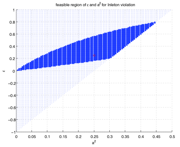
Moreover imposing positivity conditions for this matrix to correspond to a true covariance matrix gives , . Solving inequality (11) subject to these constraints yields a region of permissible and (Fig 1). In particular the point lies in this region. Interestingly enough, this example has also been discovered in the context of determinantal inequalities in [23].
Taking these results into account, we will hence study the Gaussian entropy region for 2 and 3 random variables and give the minimal number of necessary and sufficient conditions for a dimensional vector to correspond to the entropy of scalar jointly Gaussian random variables in the following sections.
III Entropy Region of 2 and 3 Gaussian Random Variables
The mentioned results in the previous section (violation of the Ingleton bound and tightness of the non-Shannon inequality) lead one to speculate whether the entropy region for arbitrary continuous random variables is equal to the entropy region of (vector-valued) Gaussian ones. Although this is the case for random variables, it is not true for . What is true for is that the entropy region of 3 arbitrary continuous random variables can be obtained from the convex cone of the region of 3 scalar-valued Gaussian random variables.
III-A
Entropy region of 2 jointly Gaussian random variables is trivially equal to the whole entropy region of 2 arbitrary distributed continuous random variables.
Theorem 4
The entropy region of 2 jointly Gaussian random variables is described by the single inequality and is equal to the entropy region of 2 arbitrary distributed continuous random variables.
Proof:
Since it is known that the continuous entropy region is described by the single balanced inequality , to prove the theorem it is sufficient to show that any entropy vector satisfying this inequality may be described by 2 jointly Gaussians and this is trivial to show.
III-B Main Results for
Although we consider vector-valued jointly Gaussian random variables, for we interestingly find that considering the convex hull of scalar jointly Gaussian random variables is sufficient for characterizing the Gaussian entropy region.
Theorem 5
The entropy region of 3 vector-valued Gaussian random variables can be obtained from the convex hull of scalar Gaussian random variables.
The main result about the convex cone of the entropy region of 3 jointly Gaussian random variables is formalized in the next theorem:
Theorem 6 (Convex Cone of the Entropy Region of 3 Scalar-Valued Gaussian Random Variables)
The convex cone generated by the entropy region of 3 scalar-valued Gaussian random variables gives the entropy region of 3 arbitrary continuously distributed random variables.
This theorem states that one can indeed construct the entropy region of continuous random variables from the entropy region of Gaussian random variables and therefore it encourages the study of Gaussians for . Moreover Theorem 6 addresses the “convex cone” of the Gaussian entropy region and as it turns out for most practical purposes characterizing the “convex cone” is sufficient. The problem of characterizing the entropy region of Gaussian random variables itself, rather than its convex cone, is more complicated. For 3 random variables we state the following conjecture:
Conjecture 1 (Entropy Region of 3 Vector-Valued Jointly Gaussian Random Variables)
Let vector defined as be an entropy vector generated by 3 vector-valued Gaussian random variables. Define and . The closure of the Gaussian entropy region generated by such vectors is characterized by,
-
1.
For :
(12) -
2.
For :
(13)
In other words we conjecture that the entropy region for three Gaussian random variables is simply given by the above inequalities. Thus, when , the Gaussian entropy region coincides with the continuous entropy region; however, when (and this can happen for some valid entropy vectors), we have the tighter upper bound (13) on . In other words the actual Gaussian entropy region for vector-valued random variables is strictly smaller than the entropy region of 3 arbitrarily distributed continuous random variables.
We strongly believe the above conjecture to be true. The missing gap in our proof is a certain function inequality, which all our simulations suggest to be true (see Conjecture 308).
III-C Proof of Main Results for
In what follows we give the proof of the results stated in the previous section for . The basic idea is to determine the structure of the Gaussian random variables that generate the boundary of the entropy region for Gaussians, and then to determine what the boundary entropies are. We need a few lemmas:
Lemma 2 (Boundary of the Gaussian Entropy Region)
The boundary of the Gaussian entropy region is generated by the concatenation of a set of vector valued Gaussian random variables with covariance
| (14) |
where the are orthogonal matrices such that , and another set of independent vector-valued Gaussian random variables with covariance
| (15) |
Proof:
To find the boundary region for 3 jointly Gaussian random variables, we can maximize linear functions of the entropy vector. We can therefore take an arbitrary set of constants and solve the following maximization problem:
| (16) |
or equivalently,
| (17) |
where is the block covariance matrix and denotes the submatrix of whose rows and columns are indexed by . We shall assume all the principal minors of are nonzero. The optimization problems (16-17) also come about when we fix any 6 of the entropies and try to maximize the last one. KKT conditions necessitate that the derivative of (17) with respect to be zero, i.e. . To compute the derivatives we note that . However since covariance matrix is symmetric, we can further write . If we adopt the following notation,
| (26) | |||
| (31) |
Then we obtain, 333Note that had we taken the derivative with respect to a symmetric matrix from the beginning, then we had, , where “diag()” denotes the diagonal elements of its argument. However this derivation would also result in equation (51).
| (44) | |||
| (51) |
Now if we assume , then we can define the following “unit-determinant” matrix:
| (55) |
Let be the submatrix of obtained from choosing rows and columns of that are indexed by . Then if we multiply (51) from left and right by we obtain:
| (65) | |||
| (76) | |||
| (84) |
Due to the special structure of , we have therefore if we define
| (85) |
and and also similar to (31), i.e.,
| (94) | |||
| (99) |
it follows that (51) will be satisfied by instead of . In other words we have the following equation:
| (109) | |||
| (113) |
Multiplying (113) by from the right we obtain,
| (126) | |||
| (139) |
Note that equating the diagonal elements to zero results in the following constraints on coefficients:
| (140) | |||
| (141) | |||
| (142) |
These imply that the equations representing the touching hyperplanes to the Gaussian region should be balanced (see Theorem 1). Now considering blocks (2,1), (3,1) together, (1,2), (3,2) with each other and (1,3), (2,3) simultaneously in (139) and noting that , we obtain
| (149) |
| (156) |
| (173) |
| (178) |
Now if the matrix were full rank, the rank of the left matrix in either of the equations (168)–(178) would be and therefore the Schur complement of its (1,1) block should be zero, i.e.:
| (179) |
in other words:
| (180) |
Since is symmetric, . This implies that off-diagonal blocks of are multiples of an orthogonal matrix, i.e.,
| (181) |
for some orthogonal matrix and such that
| (182) |
Stating (181) explicitly, we have:
| (183) | |||
| (184) | |||
| (185) |
Replacing for from (183)–(185) in equations (168)–(178) we obtain 6 equations, which turn out to be all the same as the following equation when we consider the balancedness constraints of (140)–(142) and definition of in (182):
| (186) |
Simplifying (186) using the fact that from (182), we obtain that:
| (187) |
Now note that in the general case in equations (168)–(178) need not be full rank. Therefore there is a unitary matrix such that:
| (188) |
Writing explicitly:
| (201) |
where is now full rank and we can assume its column rank (as well as its column size) to be where . This suggests doing a similarity transformation on with the following unitary matrix without affecting the block principal minors:
| (202) |
From which we obtain:
| (203) |
Considering and simultaneously and using (188) we have,
| (205) | |||
| (208) |
Therefore we can simply obtain the following structure for :
| (209) |
where the dimension of is . A similar argument for other elements yields the following structure for :
| (210) |
Now define and similar to (99) let and where for , denotes the submatrix of obtained from choosing the block rows and block columns indexed by . If we multiply (113) from the left by and from the right by , then it turns out that (113) is satisfied when are replaced . Therefore we can write equations (168)–(178) for . Doing so gives the following:
| (215) |
which if we replace for values of from (210) and assume that and represent the same value, we obtain:
| (224) |
From which it follows that:
| (225) |
Stating (225) explicitly, we have the following 3 equations:
| (230) |
| (235) |
| (240) |
Note that the dimension of is . Therefore nullity of the left matrix in (225) is at least . Hence if we let the rank of the left matrix in (225) be we will have:
| (241) |
On the other hand it is also obvious that:
| (242) |
From (241) and (242) it follows that:
| (243) |
Since a similar argument can be used for and we conclude that:
| (244) |
Now note that (230)–(240) is similar to (168)–(178) with instead of . Therefore the same argument that led to (181) yields that is a multiple of an orthogonal matrix say ; in other words
| (245) | |||
| (246) | |||
| (247) |
where similar to (182), is given by
| (248) |
and we have,
| (249) |
Note that sign of can be chosen arbitrarily in (248). Finally it follows that after a series of permutations on (210) and substituting for values of from (245)–(247), can be written as follows:
| (250) |
which if viewed as the timeshare of a set of Gaussian random variables with an orthogonal covariance matrix and another set of independent random variables, it has the same block principal minors as (210). Moreover has the same principal minors as and and therefore (250) is the optimizing solution to problem (17). However note that (250) is an optimal solution only if it is a positive semi-definite matrix. Therefore ’s and ’s should be such that,444Note that and the set of are dependent through (248). However it can be shown that for a given set of the values of can be determined such that (248) and (140)–(142) will hold.
| (251) |
| (255) |
Lemma 3 (Block Orthogonal, Block Diagonal Covariance)
Consider the covariance matrix
| (256) |
where the are orthogonal, , and in the block principal minors . Then
| (257) |
where and the upper bound is tight when and the lower bound is achieved when .
Proof:
We can easily write the following,
| (264) |
The result immediately follows from .
The and minors of the covariance matrix structure (250) obtained in Lemma 15 can now be written as,
| (265) | |||
| (266) |
Moreover since based on (249), for matrix (250), , based on Lemma 3, of (250) is given by:
| (267) |
However these values can also be obtained by a timeshare of 3 scalar random variables with covariance matrix,
| (271) |
and 3 other independent scalar random variables. This suggests that the region of 3 vector-valued Gaussian random variables may be obtained from the convex hull region of 3 scalar Gaussian random variables. In other words for , considering vector-valued random variables will not give any entropy vector that is not obtainable from scalar valued ones. This is essentially the statement of Theorem 5 and we can now proceed to a more formal proof.
Proof of Theorem 5: As in Lemma 15, we write the following optimization problem,
| (272) |
As was obtained in Lemma 15, the optimal solution is of the following form:
| (279) |
where are orthogonal matrices and . Now let
| (286) |
and define
| (293) |
However since , it follows that all blocks of are diagonal and therefore can be viwed as a timeshare of scalar random variables. Moreover since has the same principal minors as , therefore is also an optimal solution of (272).
In order to proceed to the proof of Theorem 6 we need the following lemma,
Lemma 4
Consider the function
| (294) |
where , for . is either a constant function equal to or has a unique global maximum given by:
| (295) |
Moreover if we let , then
| (296) |
Proof:
See Appendix.
Corollary 1
Let , in Lemma 4. Then is either a constant function equal to or has a unique global maximizer such that . Furthermore,
| (297) |
Now we can proceed to the proof of Theorem 6.
Proof of Theorem 6: We show that the entropy region of 3 continuous random variables can be generated from the convex cone of the Gaussian entropy region. To this end we prove that any entropy vector of 3 continuous random variables lies in the convex cone of Gaussian entropies. Let be an arbitrary entropy vector corresponding to 3 continuous random variables. We know that the only inequalities that constrain the entries of are
| (298) |
Let where the exponential acts componentwise. Then the equivalent set of constraints to (298) are
| (299) |
We now show that any such -vector can be obtained from Gaussian random variables. Consider the structure (250) obtained in Lemma 15 which suggested the time-share of a set of independent random variables with covariance matrix of block size and another set of random variables with orthogonal covariance matrix of block size . We try to find in structure (250) that will yield the desired and . Therefore if is the vector of block principal minors of structure (250) we need to obtain . Using (265) and (266) we can solve for and and obtain
| (300) |
Now we need to show that falls within the set of achievable values of . Note that calculating the determinant of the matrix in (250) via Lemma 3 or equation (267) gives
| (301) |
where the is achieved when . Letting and replacing for values of and in terms of and from (300) yields
| (302) | |||||
Of course this corresponds to the determinant of a covariance matrix of the time-share of some Gaussian random variables only if the term inside the outer parenthesis in (302) is positive. Therefore assuming and using (294) in Lemma 4:
| (303) |
It remains to show that for any given that satisfies the latter condition of (299), we have . Since by (299), can be as large as we really need to show that achieves for some value of . Therefore we need to compute,
| (304) |
Note that since we have fixed and , and that represents the timesharing of 2 sets of random variables, is not generally allowed (otherwise we enforce the random variables to be independent which is not necessarily the case for given and ). Therefore we have used instead of in (303). To find with respect to over , note that as stated in Lemma 4, has a (unique) global maximum with a value of at some . If for the assumed values of (obtained from the fixed values of and ), achives its maximum for , i.e., then
| (305) |
This immediately gives that the vector is achievable. Otherwise if , then for some , define the vector (elementwise exponentiation). This means that and hence . Now we try to achieve vector by Gaussian structure of (250). For this purpose we follow similar steps as above for and let to be the vector of block principal minors of the new corresponding matrix. Then we have
| (306) |
The global maximum of will now happen for at which it will have the value . Replacing this in (306) gives which means that although was not achievable with Gaussians is achievable. The result of the theorem is then established by noting that corresponds to a valid entropy vector , i.e., a scaled version of . Note that if maximum of happens at infinity, i.e., , then we should consider a sequence of scaled vectors (or equivalently ) where is an unbounded increasing sequence in . As , will asymptotically fall in the Gaussian region (a small perturbation of will put in the Gaussian region). Hence will belong to the closure of the convex cone of the Gaussian region as well.
Conjecture 2
Simulations of the function for different values of (Fig. 2 in the Appendix) support the statement of Conjecture 308. Our Conjecture 1 relies on the above.
Proof of Conjecture 1 Assuming Conjecture 308: To find the Gaussian entropy region again we employ Lemma 15 to obtain the boundary entropies of the region. Hence we consider the structure of (250) which is obtained from the time-share of a set of independent random variables with covariance matrix of block size and another set of random variables with orthogonal covariance matrix of block size . Let be the vector of block principal minors of the matrix in (250) and let where the exponential acts componentwise. Moreover denote the corresponding entropy vector by ( acting componentwise). Then we would like to characterize the set of -vectors (equivalently -vectors) that can arise from (250) (i.e., they lie in the convex hull of Gaussian structures). First let us investigate the constraints on and . It is easy to see that and . Therefore the imposed constraints are
| (309) |
where is due to the positivity requirement of the matrix. Next we would like to obtain the limits of . For this purpose assume that and are given fixed numbers satisfying (309). Determinant of matrix (250) is obtained from (267). If we let and substitute for and in (267) we obtain:
| (310) | |||||
Note that as described in the proof of Theorem 6, we should insist on the positivity of the expression inside the outermost parenthesis in (310). Therefore defining and using (294) in Lemma 4:
| (311) |
where since and are fixed, we have excluded and used instead of for in (311) so that we do not enforce indepndence of the underlying random variables. 555Note that if the underlying random variables are independent, then will be independent of . Using Corollary 1 and assuming that Conjecture 308 holds we obtain,
| (312) |
where . Replacing for in (312) in terms of -vector entries and using the result of (312) in (311) with the final substitution of -entries in terms of entropy elements of , yields the cojecture result. Note that when the characterization of the region is known perfectly from Corollary 1. The only part of the entropy region that is conjectured about is when whose proof relies on the validity of Conjecture 308.
IV Cayley’s Hyperdeterminant
Recall from (4) that the entropy of a collection of Gaussian random variables is simply the “log-determinant” of their covariance matrix. Similarly, the entropy of any subset of Gaussian random variables is simply the “log” of the principal minor of the covariance matrix corresponding to this subset. Therefore one approach to characterizing the entropy region of Gaussians, is to study the determinantal relations of a symmetric positive semi-definite matrix.
For example, consider 3 Gaussian random variables. While the entropy vector of 3 random variables is a 7 dimensional object, there are only 6 free parameters in a symmetric positive semi-definite matrix and therefore the minors should satisfy a constraint. It has very recently been shown that this constraint is given by Cayley’s so-called “hyperdeterminant” [20]. The hyperdeterminant is a generalization of the determinant concept for matrices to tensors and it was first introduced by Cayley in 1845 [32].
There are a couple of equivalent definitions for the hyperdeterminant among which we choose the definition through the degeneracy of a multilinear form. Consider the following multilinear form of the format in variables where each variable is a vector of length with elements in :
| (313) |
The multilinear form is said to be degenerate if and only if there is a non-trivial solution to the following system of partial derivative equations [33]:
| (314) |
The unique (up to a scale) irreducible polynomial function of entries with integral coefficients that vanishes when is degenerate is called the hyperdeterminant.
Example ( hyperdeterminant): Let and . Consider the multilinear form . The multilinear form is degenerate if there is a non-tirivial solution for such that
| (315) | |||
| (316) |
A nontirival solution exists if and only if . Therefore the hyperdeterminant is simply the determinant in this case.
The hyperdeterminant of a multilinear form was first computed by Cayley [32] and is as follows:
| (317) |
In [20] it is further shown that the principal minors of an symmetric matrix satisfy the ( times) hyperdeterminant. It is thus clear that determining the entropy region of Gaussian random variables is intimately related to Cayley’s hyperdeterminant.
It is with this viewpoint in mind that we study the hyperdeterminant in this section. In the next 2 subsections, first we present a a new determinant formula for the hyperdeterminant which may be of interest since computing the hyperdeterminant of higher formats is extremely difficult and our formula may suggest a way of attacking more complicated hyperdeterminants. Then we give a novel proof of one of the main results of [20] that the principal minors of any symmetric matrix satisfy the ( times) hyperdeterminant. Our proof hinges on identifying a determinant formula for the multilinear form from which the hyperdeterminant arises.
IV-A A Formula for the Hyperdeterminant
Obtaining an explicit formula for the hyperdeterminant is not an easy task. The first nontrivial hyperdeterminant which is the , was obtained by Cayley in 1845 [32]. However surprisingly calculating the next hyperdeterminant which is the proves to be very difficult. Until recently the only method for computing the was the nested formula of Schläfli which he had obtained in 1852 [34][33] and although after 150 years Luque and Thibon [35] expressed it in terms of the fundamental tensor invariants, the monomial expansion of this hyperdeterminant remained as a challenge. It was finally solved recently in [36] where they show that the hyperdeterminant consists of 2,894,276 terms. It is interesting to mention that Cayley had a 340 term expression for the hyperdeterminant which satisfies many invariance properties of the hyperdeterminant and only fails to satisfy a few extra conditions [37]. Therefore, as mentioned previously, computing hyperdeterminants of different formats is generally nontrivial. In fact even Schläfli’s method only works for some special hyperdeterminant formats. Moreover according to [33] it is not easy to prove directly that (IV) vanishes if and only if (314) has a non-trivial solution. Here we propose a new formula for (and a method to obtain) the hyperdeterminant which shows this is an if and only if connection directly. Moreover this method might be extendable to hyperdeterminants of larger format.
Theorem 7
(Determinant formula for hyperdeterminant) Define
Then the hyperdeterminant is given by
| (318) |
Proof:
Let be a multilinear form of the format ,
| (319) |
Then by the change of variables, , the function can be written as,
| (327) | |||||
| (329) |
To proceed, recall from (314) that the hyperdeterminant of the multilinear form of the format , vanishes if and only if there is a non-trivial solution to the system of partial derivative equations:
| (330) |
(a) First we show that if there is a non-trivial solution to the equations (330), then (318) vanishes. By the chain rule , we can write . Also from (327), . Therefore the degeneracy conditions equivalent with (330) become:
| (331) | |||||
| (333) |
Condition (331) implies that the vector should belong to the null space of the matrix . The following Lemma gives the structure of this null space.
Lemma 5
The null space of the matrix is characterized by vectors of the form, .
Proof:
Let be a vector. Noting that for , and for , , we have:
| (342) |
Solving for in the above, yields the equations:
| (344) | |||
| (345) |
Letting characterizes the vectors in the null space up to a scale:
| (347) | |||||
| (349) |
We further note that provided and , the matrix has rank 3 and that is therefore the only null space vector (up to a scaling).
Going back to the proof of Theorem 318, using Lemma 5 we conclude that we should have, and for an arbitrary non-zero scalar , . Putting these two equations into matrix form we can further write the following:
| (350) |
or in other form:
| (351) |
A non-trivial solution for and hence for requires the matrix to be low rank. Evaluating the determinant we have:
| (362) | |||||
| (368) |
Using the fact that we can write the following,
| (374) |
Note that the explicit calculation of (374) gives,
| (377) |
which when expanded gives the hyperdeterminant formula stated in equation (IV) as expected.
(b) Conversely suppose that (374) vanishes and therefore there is a non-trivial solution for and in (351). To prove that there is also a non-trivial solution to (330), we need to show that such and exist so that (331) and (333) hold. By definition of , it is not hard to see that a valid and can be found from only if in (351) has the property,
| (378) |
In the following we show that the solution of (351) in fact satisfies relation (378). Let and . Then from (351) we obtain:
| (379) | |||||
| (380) | |||||
| (381) |
Multiplying the first equation by and the second one by and adding them together we obtain,
| (382) |
which by the use of (381) simplifies to:
| (383) |
Noting that gives,
| (384) |
(378) then follows immediately from (384) by substituting for and .
IV-B Minors of a Symmetric Matrix Satisfy the Hyperdeterminant
It has recently been shown in [20] that the principal minors of a symmetric matrix satisfy the hyperdeterminant relations. There, this was found by explicitly computing the determinant of a matrix in terms of the other minors and noticing that it satisfied the hyperdeterminant. In this section we give an explanation of why this relation holds for the principal minors of a symmetric matrix. The key ingredient is identifying a simple determinant formula for the multilinear form (IV) when the coefficients are the principal minors of an symmetric matrix.
Lemma 6
Let the elements of the tensor be the principal minors of an matrix such that denotes the principal minor obtained by choosing the rows and columns of indexed by the set (by convention when all indices are zero . Then the following multilinear form of the format ( times),
| (385) |
can be rewritten as the determinant of the matrix , i.e., where is the following matrix:
| (394) |
Proof:
First note that determinant of has the form, for some -dependent coefficients (this is because each appears only in the th row of ). To prove that is in fact equal to (385), we need to show that or in other words are the corresponding minors of .
Let be a realization of . For , let the variables and the rest of the variables be zero. This choice of values makes and . Moreover it can be easily seen that in this case in (394) will simply be equal to the minor of the matrix obtained by choosing the set of rows and columns such that for all . By assumption this is nothing but the coefficient in (385) and therefore the lemma is proved.
Remark: Note that Lemma 6 does not require the matrix to be symmetric.
Lemma 7 (Partial derivatives of )
Let and . Computing the partial derivatives of gives:
| (395) | |||
| (396) |
where denotes the entry of and denotes the submatrix of obtained by choosing the rows in and columns in .
Proof:
Now we can write the condition for the minors of to satisfy the hyperdeterminant:
Lemma 8 (rank of )
The principal minors of matrix satisfy the hyperdeterminant equation if there exists a set of solutions and for which rank of in (394) is at most .
Proof:
Theorem 8 (hyperdeterminant and the principal minors)
The principal minors of an symmetric matrix satisfy the hyperdeterminants of the format ( times) for all .
Proof:
It is sufficient to show that the minors satisfy the (n times) hyperdeterminant. Recall that for the tensor of coefficients in the multilinear form (IV) to satisfy the hyperdeterminant relation, there must exist a non-trivial solution to make all the partial derivatives of with respect to its variables zero. Lemma (8) suggests that a set of nontrivial and for which rank of is at most would be sufficient.
In the following we will show that one can always find a solution to make .
First we find a non-trivial solution in the case of 3 variables and then extend it to the the case where there are variables.
For 3 variables, the matrix which is of the following form,
| (401) |
should be rank 1 or equivalently all the rows be multiples of one another. Enforcing this condition results in 3 equations for 6 unknowns. Therefore without loss of generality we let . Making the rows of proportional, gives:
| (402) | |||||
| (403) |
If , then the solution to the above equations is clearly as follows:
| (404) |
Now for the general case of variables, let be as (IV-B) and for . It can be easily checked that this solution makes the matrix of rank and therefore the principal minors satisfy the ( times) hyperdeterminant. 666Note that the solutions (IV-B) also appear in [20] in an alternative proof of principal minors satisfying the hyperdeterminant relation.
Notation 1
Each element , where , can alternatively be represented as where . For example, and .
V Minimal number of conditions for the elements of a dimensional vector to be the principal minors of a symmetric matrix for
In order to determine whether a dimensional vector corresponds to the entropy vector of scalar jointly Gaussian random variables, one needs to check whether the vector corresponds to all the principal minors of a symmetric positive semi-definite matrix. Define and let the elements of the vector be denoted by . An interesting problem is to find the minimal set of conditions under which the vector can be considered as the vector of all principal minors of a symmetric matrix. This problem is known as the “principal minor assignment” problem and has been addressed before in [20, 28]. In fact in a recent remarkable work, [20] gives the set of necessary and sufficient conditions for this problem. Nonetheless it does not point out the minimal set of such necessary and sufficient equations. Instead [20] is mainly interested in the generators of the prime ideal of all homogenous polynomial relations among the principal minors of an symmetric matrix. Here we propose the minimal set of such conditions for .
Roughly speaking there are variables in the vector and only parameters in a symmetric matrix. Therefore if the elements of can be considered as the minors of a symmetric matrix, one suspects that there should be constraints on the elements of . These constraints which can be translated to relations between the elements of the entropy vector arising from scalar Gaussian random variables, can be used as the starting point to determining the entropy region of jointly Gaussian scalar random variables.
We start this section by studying the entropy region of 4 jointly Gaussian random variables using the results of the hyperdeterminant already mentioned in the previous section and we shall explicitly state the sufficiency of 5 constraints among all the constraints given in [20] by using a similar proof to [20]; that for a given vector , and under such constraints, one can construct the symmetric matrix with the desired principle minors. Later in this section we state such minimal number of conditions for a dimensional vector for . Now define
| (407) |
Theorem 9
Let be a 15 dimensional vector whose elements are indexed by non-empty subsets of and has the property that
| (408) |
Then the minimal set of necessary and sufficient conditions for the elements of the vector to be the principal minors of a symmetric matrix consists of three hyperdeterminant equations (409–411), one consistency of the signs of (412), and the determinant identity of the matrix (413):
| (409) | |||
| (410) | |||
| (411) | |||
| (412) | |||
| (413) |
Proof:
a) It is easy to show the necessity of equations (409)–(413) and it was done in [20]. Here we illustrate the method to make the paper self-contained. Note that if elements of the vector are the principal minors of a symmetric matrix then by Theorem 8 they satisfy the hyperdeterminant relations which from (406) can be written as,
| (414) |
Using the definition of in (407), equation (414) can be further written as:
| (415) |
Therefore equations (409)–(411) simply represent the hyperdeterminant relations and hold by Theorem 8. Moreover if is the principal minor of matrix obtained by choosing rows and columns , and , then writing in terms of the entries of gives,
| (416) | |||||
where since corresponds to principal minors of , we have substituted for and . Rewriting (416) we obtain,
| (417) |
which by comparison to (407) means that the following holds,
| (418) |
Therefore replacing for and from (418) in (412) and simplifying we obtain that (412) holds trivially. The last condition (413) is also nothing but the expansion of the determinant of in terms of the entries of and replacing for them in terms of and lower order minors and therfore is a necessary condition.
b) Now we need to show the sufficiency of equations (409)–(413). To do so, we assume that the given vector satisfies (409)–(413) and we want to show that it is the principal minor vector of some symmetric matrix . Hence we try to construct a matrix whose principal minors are given by the entries of vector . First note that such a matrix should have and (or equivalently ). The only ambiguity in fully determining the entries of will therefore be the signs of the off-diagonal entries. To have the minors of also equal to the corresponding entries of vector , we should have:
| (422) | |||||
| (423) |
Replacing for values of and in terms of and we obtain that,
| (424) |
Therefore writing the condition for all we need to have
| (425) | |||
| (426) | |||
| (427) | |||
| (428) |
Note that the constraints (409)–(412) guarantee that . It remains to show that there is a consistent choice of signs for such that the stronger condition also holds. Note that without loss of generality we can assume that the off-diagonal entries on the first row, i.e., are positive. This is due to the fact that we can use the transformation where is a diagonal matrix with elements to make positive without affecting any of the principal minors. Hence, assuming are positive, the signs of and are determined from the signs of and in (425–427). However once the signs of and are determined, the sign of their product, i.e., should be the same as the sign of to satisfy (428). This is enforced by equation (412). Therefore conditions (409)–(412) yield (425)–(428). Note that due to property (408) none of the are zero and hence all the above steps for sign choice are valid. Finally a direct calculation of the determinant of shows that it can be expressed as the right-hand side of equation (413) in terms of lower order minors of which are equal to corresponding terms . Consequently equation (413) guarantees that the principal minor of is equal to . Again note that since property (408) holds, the denominator in (413) is nonzero and will not cause any problems. Therefore will be the matrix with principal minors given by vector .
Using a similar approach which follows the proof methods of [20] closely, we can write the set of minimal necessary and sufficient conditions for a dimensional vector to be the principal minors of a symmetric matrix.
Theorem 10
Let be a dimensional vector whose elements are indexed by non-empty subsets of (assume ) and that it satisfies,
| (429) |
Then the necessary and sufficient conditions for a dimensional vector to be the principal minors of a symmetric matrix consists of equations and are as follows,
| (430) | |||
| (431) |
Also choose one set of such that and let ,
| (432) |
where is obtained from the following by replacing every by .
| (433) |
Proof:
The proof is essentially the same as the proof technique of [20] and is a generalization of Theorem 9 to a dimensional vector. However we would like to highlight why (430)–(432) is the minimal set of necessary and sufficient conditions among all conditions given in [20]. First consider the necessitiy of the equations:
a) Showing the necessity of equations (430)–(432) is strightforward. In fact if the elements of vector are the principal minors of a symmetric matrix , then and . Furthermore it can be shown (similar to the proof of Theorem 9) that from which it follows that (430)–(431) hold. Note that in equation (433) gives in terms of lower order minors (compare to equation (413)). Now consider a submatrix of whose rows and column are indexed by and denote it by . For let and likewise let the submatrix with rows and columns indexed by be shown by . Further denote the Schur complement of in by . Note that is a matrix whose determinant can be obtained via the rule of equation (433). The property of Schur complement yields,
| (434) |
Therefore wiritng the determinant for the matrix and using (434), gives equation (432). 777Note that we can assume and simply avoid .
b) To show the sufficiency we show that if a given vector satisfies equations (430)–(432) then we can construct a symmetric matrix whose principal minors are given by . As we did in Theorem 9 such a matrix should have entries and (or equivalently ). Therefore it remains to choose the signs of the off-diagonal entries in a consistent fashion so that all the minors of will correspond to .
For minors of to comply with , note that as was obtained in Theorem 9, we need to have . Note that equations (430)–(432) give that for all . Again similar to Thereom 9, we may assume that all the off-diagonal terms in the first row are positive since we can always use the transformation where is a diagonal matrix with elements to make positive. Therefore assuming are positive, we can choose the sign of all off-diagonal terms such that they have the same sign as . This way we guarantee . However note that all the signs of all entries of are now fixed and therefore we need to make sure the remaining conditions for all are also satisfied. However since and satisfies the constraint (431) as well, for follows immediately. Therefore equations (430) and (431) guarantee the equality of minors of with the corresponding entries of . Note that property (429) assures that none of the are zero and hence all the above steps for determining the sign will be valid.
Now we need to prove the equality of all minors of size and bigger of with the relative entries of . This is enforced by condition (432). To see the reason, replace each term in (432) by . Then as we saw in part (a), the resulting equation describes in terms of lower order minors which are already guaranteed to be equal to the corresponding entries of . Therefore condition (432) is enforcing . Note that for each only 1 equation of type (432) is required. Moreover due to property (429) the denominators in (432) obtained from (433) will be nonzero and will not cause any problems.
Corollary 2
Remark: Note that in order to characterize the entropy region of scalar Gaussian random variables what one really needs is the convex hull of all such entropy vectors. After all if we only wanted to determine whether 7 numbers correspond to the entropy vector of 3 scalar-valued jointly Gaussian random variables we could simply check whether they satisfy the hyperdeterminant relation (406). However it is the convex hull which is more interesting, and more cumbersome to calculate, and this is what we addressed for 3 random variables in Section III.
VI Discussions and Conclusions
In this paper, we studied the entropy region of jointly Gaussian random variables as an interesting subclass of continuous random variables. In particular we determined that the whole entropy region of 3 arbitrary continuous random variables can be obtained from the convex cone of the entropy region of 3 scalar-valued jointly Gaussian random variables. We also gave the representation of the entropy region of 3 vector-valued jointly Gaussian random variables through a conjecture.
We should remark that, in general, to characterize the entropy region of Gaussian random variables one should consider vector-valued random variables which is probably more complex than the case of scalars. In Section III we showed that, for , the vector-valued random variables do not result in a bigger region than the convex hull of scalar ones. However in general it is not known whether the entropy region of vector-valued jointly Gaussian random variables is greater than the convex hull of the entropy region of scalar valued Gaussians.
For we explicitly stated the set of constraints that a dimensional vector should satisfy in order to correspond to the entropy vector (equivalently the vector of all principal minors) of scalar jointly Gaussian random variables. Although these conditions allow one to check whether a real vector of numbers corresponds to an entropy vector of scalar jointly Gaussian random variables, they do not reveal if such given vector of real numbers corresponds to the entropy vector of vector-valued Gaussian random variables or if it lies in the convex hull of scalar Gaussian entropy vectors. Answering these question requires one to study the region of vector valued jointly Gaussian random variables and this is what we addressed in Section III for 3 random variables. Obtaining the entropy region of vector-valued Gaussians seems to be rather complicated for and as a satrting point one may instead focus on the convex hull of scalar Gaussians which is essentially the convex hull of vectors satisfying constraints (430)–(432). Studying such a convex hull has an interesting connection to the concept of an “amoeba” in algebraic geometry. The “amoeba” of a polynomial is defined as the image of in under the mapping [33]. It turns out that many properties of amoebas can be deduced from the Newton polytope of which is defined as the convex hull of the exponent vectors in (see, e.g., [38]). In terms of our problem of interest, the scalar Gaussian entropy points are the intersection of the amoebas associated to polynomials (430)-(432) and one should look for the convex hull of the locus of these intersection points. If we allow the notion of amoeba to be defined as the mapping for any function (not just polynomials), then one could also formulate our problem of interest as the convex hull of the amoeba of the algebraic variety obtained from the intersection of (430)-(432).
Finally in characterizing the entropy region of Gaussian random variables for , we noted the important role of the hyperdeterminant and with this viewpoint we also examined the hyperdeterminant relations. In particular by giving a determinant formula for a multilinear form, we gave a transparent proof that the hyperdeterminant relation is satisfied by the principal minors of an symmetric matrix. Moreover we also obtained a determinant form for the hyperdeterminant which might be extendible to higher order formats and is an interesting problem even in its own right.
Appendix
Proof of Lemma 4
Proof: We will first show that . Let,
| (435) |
For distinct , this can also be written as,
| (436) | |||||
| (437) |
which shows and therefore for all , with equality if and only if or equivalently,
| (438) |
Note that this is only possible when . Without loss of generality assume, , and define,
| (439) |
Clearly zeros of determine the global maximums of (i.e., ). Therefore we analyze the behavior of in the following scenarios (based on the assumption ):
-
1.
:
Note that for any number , when , we have the approximation, . Therefore as , we obtain,(440) On the other hand when , we have . Therefore has at least one zero (which is not at origin). In fact we now show that it has exactly one zero. Let . Then zeros of and match except possibly at infinity. Therefore we can equivalently determine the zeros of . To do so, we further define . Note that as , . Moreover as we obtain . On the other hand obtaining the derivative of gives,
(441) which has a unique zero at,
(442) Calculating shows that has a maximum at . Noting that derivative of is defined for all yet it is only zero at and that and , we conclude that has exactly one zero at some . Since we defined , we obtain that has also exactly one zero at (and is also possibly zero at infinity). Moreover we have , , and . Since is also everywhere differentiable we deduce that has exactly one zero (that is not at origin) at some where . Finally going back to , we obtain that starts at origin, i.e., however with a negative slope . It has a unique zero at and it approaches the -axis again at infinity with a positive sign, i.e., as . Therefore we have shown that ’s behavior is as the one depicted in Fig. 2(a).
Note that since the zeros of determine the global maximums of , to determinne where the global maximums of occur, we need to calculate at and . First for we have,
(443) Moreover for we have for . Therefore we can write,
(444) (445) Since and , the term will be the dominant term and we will have,
(446) Therefore as we obtain . As a result has a unique global maximizer at where . Note in Fig. 2(a) that the zero of coincides with the maximum of .

Figure 2: Functions and versus . The solid line shows function and the dashed line shows function . -
2.
:
In this case we have . Similar to the previous case we define and analyze the zeros of . Note that which has a unique zero at the point given by,
(447) Since as and and again is everywhere differnetiable, we obtain that has exactly one zero (that is not at origin) at some where . Therefore has also exactly one zero (that is not at origin) at . Again we have as and and hence its behavior is again as the one depicted in Fig. 2(b).
The analysis of and is similar to the last case. In particular we have, and giving for . Hence has a unique maximizer at such that . Again it is evident from Fig. 2(b) that the zero of coincides with the maximum of .
-
3.
:
In this case . Calculating which has a unique zero at given by,
(448) Moreover as we have and as , . Therefore the behavior of in this case is as shown in Fig. 2(c).
The analysis of and is again similar to the previous 2 cases. However note that in this case the only zero of is at origin and as a result we only need to consider the value of at and infinity. Following a similar procedure as in the previous cases, we obtain and for by replacing in (445) we get,
(449) Therefore , i.e., approaches its global maximum at infinity.
-
4.
:
In this case, and we have which again has a unique zero at given by, . As in the previous case, and and behaves as in the previous case (Fig. 2(d)).
Since zeros of happen at and infinity, we only need to calculate the value of at 0 and infinity. For we have, . On the other hand by replacing in (445) we obtain as ,
(450) This yields as . As a result again approaches its global maximum at infinity.
-
5.
:
In this case simplifies to . Note that and is an increasing function. The behavior of is shown in Fig. 2(e).
Since the zero of occurs at zero, we only need to evaluate at zero for which we obtain and therefore , i.e., the global maximum of is at zero.
-
6.
:
In this case we have . Behavior of is shown in Fig. 2(f).
For this scenario again we only need to care for which can be easily obtained to be which is the global maximum.
-
7.
:
Here we obtain a constant function. To evaluate we do not need to use in this case. In fact we have which is a constant function as well and equal to its global maximum everywhere.
Thus far we showed that (except for the case when and is a constant) it has a unique global maximizer at which . Moreover in all these cases, if for some we have it can be seen that maximum of occurs for some . Noting that as defined in the statement of the theorem is in fact , it immediately follows that if then attains its global maximum for some .
References
- [1] B. Hassibi and S. Shadbakht, “The entropy region for three gaussian random variables,” in IEEE Int. Symp. on Inf. Theory (ISIT), 2008.
- [2] S. Shadbakht and B. Hassibi, “Cayley’s hyperdeterminant, the principal minors of a symmetric matrix and the entropy region of 4 Gaussian random variables,” 46th Annual Allerton Conf. on Comm., Control, and Computing, Monticello, IL, 2008.
- [3] B. Hassibi and S. Shadbakht, “Normalized entropy vectors, network information theory and convex optimization,” in Information theory workshop, Bergen, Norway, 2007.
- [4] X. Yan, R.W. Yeung, and Z. Zhang, “The capacity region for multi-source multi-sink network coding,” in IEEE Int. Symp. on Inf. Theory (ISIT), 2007, pp. 116–120.
- [5] R.W. Yeung, “A framework for linear information inequalities,” IEEE Trans. on Information Theory, vol. 43, no. 6, pp. 1924–1934, 1997.
- [6] F. Matus, “Infinitely many information inequalities,” in IEEE Int. Symp. on Inf. Theory (ISIT), 2007, pp. 41–44.
- [7] Zhen Zhang and Raymond Yeung, “A non-shannon-type conditional inequality of information quantities,” IEEE Trans. on Information Theory, vol. 43, no. 6, pp. 1982–1986, 1997.
- [8] R. Dougherty, C. Freiling, and K. Zeger, “Six new non-shannon information inequalities,” in IEEE Int. Symp. on Inf. Theory (ISIT), 2006, pp. 233–236.
- [9] T.H. Chan and R.W. Yeung, “On a relation between information inequalities and group theory,” IEEE Trans. on Information Theory, vol. 48, no. 7, pp. 1992–1995, 2002.
- [10] T.H. Chan, “A combinatorial approach to information inequalities,” Communications In Information and Systems, vol. 1, no. 3, pp. 241–254, 2001.
- [11] K. Makarychev, Y. Makarychev, A. Romashchenko, and N. Vereshchagin, “A new class of non-shannon-type inequalities for entropies,” Communications In Information and Systems, vol. 2, no. 2, pp. 147–166, 2002.
- [12] Z. Zhang, “On a new non-Shannon type information inequality,” Communications In Inf. and Systems, vol. 3, no. 1, pp. 47–60, 2003.
- [13] B. Hassibi and S. Shadbakht, “On a construction of entropic vectors using lattice-generated distributions,” in IEEE Int. Symp. on Inf. Theory (ISIT), 2007, pp. 501–505.
- [14] Z. Zhang and R. Yeung, “On characterization of entropy function via information inequalities,” IEEE Trans. on Information Theory, vol. 44, no. 4, pp. 1440–1452, 1998.
- [15] F. Matus and M. Studeny, “Conditional independences among four random variables I,” Combin., Prob. Comput., vol. 4, pp. 269–278, 1995.
- [16] S. Fujishije, “Polymatroidal dependence structure of a set of random variables,” Information and Control, vol. 39, pp. 55–72, 1978.
- [17] T. S. Han, “A uniqueness of shannon’s information distance and related nonnegativity problems,” J. Comb.,Inform. Syst. Sci., vol. 6, no. 4, pp. 320–331, 1981.
- [18] F. Matus, “Two constructions on limits of entropy functions,” IEEE Trans. on Information Theory, vol. 53, no. 1, pp. 320–330, 2007.
- [19] T. H. Chan, “Balanced information inequalities,” IEEE Trans. on Information Theory, vol. 49, no. 12, pp. 3261–3267, 2003.
- [20] O. Holtz and B. Sturmfels, “Hyperdeterminantal relations among symmetric principal minors,” Journal of Algebra, vol. 316, pp. 634–648, 2007.
- [21] T. M. Cover and J. A. Thomas, “Determinant inequalities via information theory,” SIAM J. Matrix Anal. Appl., vol. 9, no. 3, pp. 384–392, 1988.
- [22] Shaun M. Fallat and Charles R. Johnson, “Determinantal inequalities: Ancient history and recent advances,” Contemporary Mathematics, vol. 259, pp. 199–211, 2000.
- [23] Charles R. Johnson and Wayne W. Barrett, “Determinantal inequalities for positive definite matrices,” Discrete Mathematics, vol. 119, pp. 97–106, 1993.
- [24] H. T. Hall and C. R. Johnson, “Bounded ratios of products of principal minors of positive definite matrices,” arXiv:0806.2645v1.
- [25] R. Lněnička and F. Matúš, “On gaussian conditional independence structures,” Kybernetika, vol. 43, no. 3, pp. 327–342, 2007.
- [26] K. Griffin and M. J. Tsatsomeros, “Principaal minors, part i: A method for computing all the principal minors of a matrix,” Linear Algebra and its applications, vol. 419, no. 1, pp. 107–124, 2006.
- [27] Radim Lnenicka, “On the tightness of the Zhang-Yeung inequality for gaussian vectors,” Communications in information and systems, vol. 3, no. 1, pp. 41–46, 2003.
- [28] K. Griffin and Tsatsomeros M. J, “Principal minors, part II: The principal minor assignment problem,” Linear Algebra and its applications, vol. 419, pp. 125–171, 2006.
- [29] A. W. Ingleton, “Representation of matroids,” in Combinatorial mathematics and its applications, D. Welsh, Ed. London: Academic Press, 1971, pp. 149–167.
- [30] T. H. Chan, “Capacity region for linear and Abelian network codes,” in Information theory and applications workshop, San Diego, CA, 2007.
- [31] T. H. Chan, “Group characterizable entropy functions,” in IEEE Int. Symp. on Inf. Theory (ISIT), 2007, pp. 506–510.
- [32] A. Cayley, “On the theory of linear transformations,” in Cambridge Math. J. 4, 1845, pp. 1–16.
- [33] I. M. Gelfand, M. M. Kapranov, and A. V. Zelevinsky, Discriminants, resultants and multidimensional determinants, Mathematics: Theory and Applications., 1994.
- [34] L. Shläfli, “Über die resultante eines systemes mehrerer algebraischen gleichungen,” Denkschr. der Kaiserlichen Akad. der Wiss., Math-Naturwiss. Klasse, vol. 4, 1852.
- [35] J-G Luque and J-Y Thibon, “Polynomial invariants of four qubits,” Phys. Rev. A 67, 042303, 2003.
- [36] Peter Huggins, Bernd Sturmfels, Josephine Yu, and Debbie S. Yuster, “The hyperdeterminant and triangulations of the 4-cube,” Mathematics of Computation, vol. 77, no. 263, pp. 1653–1679, 2008.
- [37] S. P Tsarev and T. Wolf, “Hyperdeterminants as integrable discrete systems,” J. Phys. A: Math Theor, vol. 42, no. 45, 2009.
- [38] M. Passare and H. Rullgård, “Amoebas. Monge-Ampère measures, and triangulations of the newton polytope,” Duke Math. J., vol. 121, no. 3, pp. 481–507, 2004.