Local Naive Bayes Nearest Neighbor for Image Classification

Abstract

We present Local Naive Bayes Nearest Neighbor, an improvement to the NBNN image classification algorithm that increases classification accuracy and improves its ability to scale to large numbers of object classes. The key observation is that only the classes represented in the local neighborhood of a descriptor contribute significantly and reliably to their posterior probability estimates. Instead of maintaining a separate search structure for each class, we merge all of the reference data together into one search structure, allowing quick identification of a descriptor’s local neighborhood. We show an increase in classification accuracy when we ignore adjustments to the more distant classes and show that the run time grows with the log of the number of classes rather than linearly in the number of classes as did the original. This gives a 100 times speed-up over the original method on the Caltech 256 dataset. We also provide the first head-to-head comparison of NBNN against spatial pyramid methods using a common set of input features. We show that local NBNN outperforms all previous NBNN based methods and the original spatial pyramid model. However, we find that local NBNN, while competitive with, does not beat state-of-the-art spatial pyramid methods that use local soft assignment and max-pooling.

1 Introduction

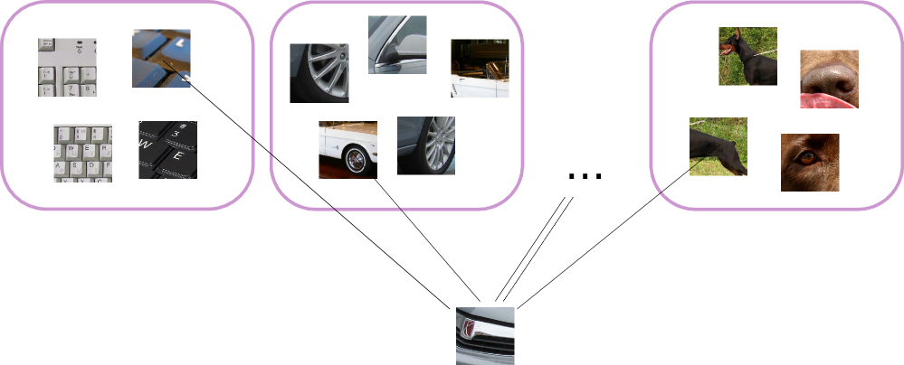
(a) The original NBNN asks, “Does this descriptor look like a keyboard? a car? … a dog?”

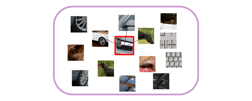
(b) Local NBNN asks, “What does this descriptor look like?”

Figure 1: Instead of considering classes individually, we search one merged index.

A widely used approach to object category recognition has been the bag-of-words method [7] combined with the spatial pyramid match kernel [14]. This approach uses visual feature extraction, quantizes features into a limited set of visual words, and performs classification, often with a support vector machine [12, 13].

In contrast to the bag-of-words method, Boiman et al. [3] introduced a feature-wise nearest neighbor algorithm called Naive Bayes Nearest Neighbor (NBNN). They do not quantize the visual descriptors and instead retain all of the reference descriptors in their original form.

Boiman et al. [3] showed that quantizing descriptors in the bag-of-words model greatly decreases the discriminativity of the data. The bag-of-words model usually reduces the high dimensional feature space to just a few thousand visual words.

Despite NBNN’s independence assumption (independence of the descriptors in the query image), Boiman et al. demonstrated state-of-the-art performance on several object recognition datasets, improving upon the commonly used SVM classifier with a spatial pyramid match kernel.

NBNN is a simple algorithm. The task is to determine the most probable class $\hat{C}$ of a query image $Q$. Let $d_{1},\ldots,d_{n}$ be all the descriptors in the query image. The training data for a class is a collection of descriptors extracted from a set of labelled example images. These are stored in data structures that allow for efficient nearest neighbor searches (the nearest neighbor of descriptor $d_{i}$ in class $C$ is $\operatorname{NN}_{C}(d_{i})$). The original NBNN is listed as Algorithm 1.

Algorithm 1 $\mbox{\sc NBNN}(Q)$ [3]

0:  A nearest neighbor index for each $C$, queried using ${\rm NN}_{C}()$.

0:  A query image $Q$, with descriptors $d_{i}$.

  for all descriptors $d_{i}\in Q$ do

     for all classes $C$ do

        ${\rm totals}[C]\leftarrow{\rm totals}[C]+\|d_{i}-{\rm NN}_{C}(d_{i})\|^{2}$

     end for

  end for

  return  $\operatornamewithlimits{argmin}_{C}{\rm totals}[C]$

Our contribution is a modification to the original NBNN algorithm that increases classification accuracy and provides a significant speed-up when scaling to large numbers of classes. We eliminate the need to search for a nearest neighbor in each of the classes. Instead, we merge the reference datasets together and use an alternative nearest neighbor search strategy in which we only adjust the scores for the classes nearest to any query descriptor. The question becomes, “What does this descriptor look like?”, instead of “Does this descriptor look like one from a car? a duck? a face? a plane? …” Figure 1 gives a conceptual visualization.

We also provide the first head-to-head comparison of NBNN based methods with spatial pyramid methods using a common feature set. Previous work [3, 19] has only provided comparisons with published figures while extracting different feature sets for their experiments.

2 Relation to previous work

An obvious issue with the naive Bayes approach is that it makes the unrealistic assumption that image features provide independent evidence for an object category.

In defense of the naive Bayes assumption, Domingos and Pazzani [9] demonstrate the applicability of the naive Bayes classifier even in domains where the independence assumption is violated. They show that while the independence assumption does need to hold in order for the naive Bayes classifier to give optimal probability estimates, the classifier can perform well as regards misclassification rate even when the assumption doesn’t hold. They perform extensive evaluations on many real-world datasets that violate the independence assumption and show classification performance on par with or better than other learning methods.

Behmo et al. [2] corrects NBNN for the case of unbalanced training sets. Behmo et al. implemented and compared a variant of NBNN that used $n$ 1-vs-all binary classifiers, highlighting the effect of unbalanced training data. In the experiments we present, the training sets are approximately balanced, and we compare our results to the original NBNN algorithm. Behmo et al. also point out that a major practical limitation of NBNN is the time that is needed to perform the nearest neighbor search, which is what our work addresses.

The most recent work on NBNN is by Tuytelaars et al. [19]. They use the NBNN response vector of a query image as the input features for a kernel SVM. This allows for discriminative training and combination with other complimentary features by using multiple kernels. The kernel NBNN gives increased classification accuracy over using the basic NBNN algorithm. Our work is complimentary to this in that the responses resulting from our local NBNN could also be fed into their second layer of discriminative learning. Due to the poor scaling of the original NBNN algorithm, Tuytelaars et al. had to heavily subsample the query images in order to obtain timely results for their experiments, hampering their absolute performance values. In NBNN, what dominates is the time needed to search for nearest neighbors in each of the object category search structures. Even approximate methods can be slow here and scale linearly with the number of categories.

The method we will introduce is a local nearest neighbor modification to the original NBNN. Other methods taking advantage of local coding include locality constrained linear coding by [20] and early cut-off soft assignment by [15]. Both limit themselves to using only the local neighborhood of a descriptor during the coding step. By restricting the coding to use only the local dictionary elements, these methods achieve improvements over their non-local equivalents. The authors hypothesize this is due to the manifold structure of descriptor space, which causes Euclidean distances to give poor estimates of membership in codewords far from descriptor being coded [15].

NBNN methods can be compared to the popular spatial pyramid methods [4, 14, 20], which achieve state-of-the-art results on image categorization problems. The original spatial pyramid method used hard codeword assignment and average pooling within each of the hierarchical histogram bins. Today, the best performing variants of spatial pyramid use local coding methods combined with max pooling [4, 5, 15, 20]. State-of-the-art spatial pyramid methods achieve high accuracy on benchmark datasets, but there has been no head-to-head comparison of NBNN methods against spatial pyramid methods. Previous work has only compared against published figures, but these comparisons are based on different feature sets, which makes it difficult to isolate the contributions of the features from the contributions of the methods.

3 Naive Bayes Nearest Neighbor

To help motivate and justify our modifications to the NBNN algorithm, this section provides an overview of the original derivation [3]. Each image $Q$ is classified as belonging to class $\hat{C}$ according to

$$\hat{C}=\operatornamewithlimits{argmax}_{C}p(C|Q).$$ (1)

Assuming a uniform prior over classes and applying Bayes’ rule,

$$\hat{C}=\operatornamewithlimits{argmax}_{C}\log(p(Q|C)).$$ (2)

The assumption of independence of the descriptors $d_{i}$ found in image $Q$ gives

$$\hat{C} =\operatornamewithlimits{argmax}_{C}\left[\log(\prod_{i=1}^{n}p(d_{i}|C))\right]$$ (3)

$$=\operatornamewithlimits{argmax}_{C}\left[\sum_{i=1}^{n}\log p(d_{i}|C)\right].$$ (4)

Next, approximating $p(d_{i}|C)$ in Equation 4 by a Parzen window estimator, with kernel $K$, gives

$$\hat{p}(d_{i}|C)=\frac{1}{L}\sum_{j=1}^{L}K(d_{i}-d_{j}^{C})$$ (5)

where there are $L$ descriptors in the training set for class $C$ and $d_{j}^{C}$ is the $j$-th nearest descriptor in class $C$. This can be further approximated by using only the $r$ nearest neighbors as

$$\hat{p}_{r}(d_{i}|C)=\frac{1}{L}\sum_{j=1}^{r}K(d_{i}-d_{j}^{C})$$ (6)

and NBNN takes this to the extreme by using only the single nearest neighbor ($\operatorname{NN}_{C}(d_{i})$):

$$\hat{p}_{1}(d_{i}|C)=\frac{1}{L}K(d_{i}-\operatorname{NN}_{C}(d_{i})).$$ (7)

Choosing a Gaussian kernel for $K$ and substituting Equation 7 (the single nearest neighbor approximation of $p(d_{i}|C)$) into Equation 4 (the sum of log probabilities) gives:

$$\hat{C} =\operatornamewithlimits{argmax}_{C}\left[\sum_{i=1}^{n}\log\frac{1}{L}e^{-\frac{1}{2\sigma^{2}}\|d_{i}-\operatorname{NN}_{C}(d_{i})\|^{2}}\right]$$ (8)

$$=\operatornamewithlimits{argmin}_{C}\left[\sum_{i=1}^{n}\|d_{i}-\operatorname{NN}_{C}(d_{i})\|^{2}\right].$$ (9)

Equation 9 is the NBNN classification rule: find the class with the minimum distance from the query image.

4 Towards local NBNN

Before introducing local NBNN, we first present some results demonstrating that we can be selective with the updates that we choose to apply for each query descriptor. We start by re-casting the NBNN updates as adjustments to the posterior log-odds of each class. In this section, we show that only the updates giving positive evidence for a class are necessary.

The effect of each descriptor in a query image $Q$ can be expressed as a log-odds update. This formulation is useful because it allows us to restrict updates to only those classes for which the descriptor gives significant evidence. Let $C$ be some class and $\overline{C}$ be the set of all other classes.

The odds ($\mathcal{O}$) for class $C$ is given by

$$\mathcal{O}_{C} =\frac{P(C|Q)}{P(\overline{C}|Q)}$$ (10)

$$=\frac{P(Q|C)P(C)}{P(Q|\overline{C})P(\overline{C})}$$ (11)

$$=\prod_{i=1}^{n}\frac{P(d_{i}|C)}{P(d_{i}|\overline{C})}\frac{P(C)}{P(\overline{C})}.$$ (12)

Taking the log and applying Bayes’ rule again gives:

$$\log(\mathcal{O}_{C}) =\sum_{i=1}^{n}\log\frac{P(d_{i}|C)}{P(d_{i}|\overline{C})}+\log\frac{P(C)}{P(\overline{C})}$$ (13)

$$=\sum_{i=1}^{n}\underbrace{\log\frac{P(C|d_{i})P(\overline{C})}{P(\overline{C}|d_{i})P(C)}}_{\text{increment}}+\underbrace{\log\frac{P(C)}{P(\overline{C})}}_{\text{prior}}.$$ (14)

Equation 14 has an intuitive interpretation. The prior odds are $P(C)/P(\overline{C})$. Each descriptor then contributes a change to the odds of a given class determined by the posterior odds of $C$ given $d_{i}$, $P(C|d_{i})/P(\overline{C}|d_{i})$, and how they differ from the prior odds as seen in the increment term of Equation 14. If the posterior odds are equal to the prior odds, $\text{increment}=0$, if the posterior odds are greater than the prior odds, $\text{increment}>0$, and if the posterior odds are less than the prior odds, the $\text{increment}<0$.

This allows an alternative classification rule that’s expressed in terms of log-odds increments:

$$\hat{C}=\operatornamewithlimits{argmax}_{C}\left[\sum_{i=1}^{n}\log\frac{P(C|d_{i})P(\overline{C})}{P(\overline{C}|d_{i})P(C)}+\log\frac{P(C)}{P(\overline{C})}\right]$$ (15)

where the prior term can be dropped if you assume equal class priors. The increment term is simple to compute if we leave $P(C|d_{i})\propto e^{-\|d_{i}-\operatorname{NN}_{C}(d_{i})\|^{2}}$ as in the original.

The benefit that comes from this formulation is that we can be selective about which increments to actually use: we can use only the significant log-odds updates. For example, we can decide to only adjust the class posteriors for which the descriptor gives a positive contribution to the sum in Equation 15. Table 1 shows that this selectivity does not affect classification accuracy.

Method	Avg. # increments	Accuracy %
Full NBNN	101	55.2 $\pm 0.97$
Positive increments only	55.0	55.6 $\pm 1.17$

Table 1: Effect of restricting increments to only the positive increments on a downsampled version (128x128) of the Caltech 101 dataset. The $\pm$ shows one standard deviation.

5 Local NBNN

The selectivity introduced in the previous section shows that we do not need to update each class’s posterior for each descriptor. This section shows that by focusing on a much smaller, local neighborhood (rather than on a particular log-odds threshold), we can use an alternate search strategy to speed up the algorithm, and also achieve better classification performance by ignoring the distances to classes far from the query descriptor.

Instead of performing a search for a query descriptor’s nearest neighbor in each of the classes’ reference sets, we search for only the nearest few neighbors in a single, merged dataset comprising all the features from all labelled training data from all classes. Doing one approximate k-nearest-neighbor search in this large index is much faster than querying each of the classes’ approximate-nearest-neighbor search structures. This is a result of the sublinear growth in computation time with respect to index size for approximate nearest neighbor search algorithms as discussed in Section 5.1. This allows the algorithm to scale up to handle many more classes, avoiding a prohibitive increase in runtime.

This is an approximation to the original method. For each test descriptor in a query image, we do not find a nearest neighbor from every class, only a nearest neighbor from classes that are represented in the $k$ nearest descriptors to that test descriptor. We call this local NBNN, visualized in Figure 2.

Figure 2: NBNN finds the nearest neighbor from each of the classes (the shapes, in this figure). Local NBNN retrieves only the local neighborhood, finding nearest neighbors from only some of the classes. The shaded descriptors are those that would be used for updating the distance totals. We only use the closest member from any class, and don’t find an example from each class.

It is important to properly deal with the set of background classes which were not found in the $k$ nearest neighbors of $d$. To handle the classes that were not found in the $k$ nearest neighbors, we conservatively estimate their distance to be the distance to the $k+1$-st nearest neighbor (this can be thought of as an upper bound on the density of background features). In practice, instead of adjusting the distance totals to every class, it is more efficient to only adjust the distances for the relatively few classes that were found in the $k$ nearest neighbors, but discount those adjustments by the distance to background classes (the $k$+1st nearest neighbor). This does not affect the minimum.

The local NBNN algorithm is as follows:

Algorithm 2 $\mbox{\sc LocalNBNN}(Q,k)$

0:  A nearest neighbor index comprising all descriptors, queried using ${\rm NN}({\it descriptor},{\it\#neighbors})$.

0:  A class lookup, ${\rm Class}({\it descriptor})$ that returns the class of a descriptor.

  for all descriptors $d_{i}\in Q$ do

     $\{p_{1},p_{2},\ldots,p_{k+1}\}\leftarrow{\rm NN}(d_{i},k+1)$

     ${\it dist}_{B}\leftarrow\|d_{i}-p_{k+1}\|^{2}$

     for all categories $C$ found in the $k$ nearest neighbors do

        ${\it dist}_{C}=\min_{\{p_{j}|{\rm Class}(p_{j})=C\}}\|d_{i}-p_{j}\|^{2}$

        ${\rm totals}[C]\leftarrow{\rm totals}[C]+{\it dist}_{C}-{\it dist}_{B}$

     end for

  end for

  return  $\operatornamewithlimits{argmin}_{C}{\rm totals}[C]$

5.1 Approximate nearest neighbors and complexity

Our algorithm scales with the log of the number of classes rather than linearly in the number of classes. This analysis depends on the nearest neighbor search structure that we use.

For both our implementation of the original NBNN and local NBNN, we use FLANN [17] to store descriptors in efficient approximate nearest neighbor search structures. FLANN is a library for finding approximate nearest neighbor matches that is able to automatically select from among several algorithms and tune their parameters for a specified accuracy. It makes use of multiple, randomized KD-trees as described by Silpa-Anan and Hartley [18] and is faster than single KD-tree methods like ANN [1] (used by Boiman et al. in the original NBNN) or locality sensitive hashing methods. The computation required and the accuracy of the nearest neighbor search is controlled by the number of leaf nodes checked in the KD-trees.

Following the analysis by Boiman et al. [3], let $N_{T}$ be the number of training images per class, $N_{C}$ the number of classes, and $N_{D}$ the average number of descriptors per image. In the original, each KD-tree contains $N_{T}N_{D}$ descriptors and each of the $N_{D}$ query descriptors requires an approximate search in each of the $N_{C}$ KD-tree structures. The accuracy of the approximate search is controlled by the number of distance checks, $c$. The time complexity for processing one query image under the original algorithm is $O(cN_{D}N_{C}\log(N_{T}N_{D}))$. In our method, there is a single search structure containing $N_{D}N_{C}N_{T}$ descriptors in which we search for $k$ nearest neighbors (using $c$ distance checks, where $c\gg k$). The time complexity for processing one query image under our method is $O(cN_{D}\log(N_{C}N_{T}N_{D}))$. The $N_{C}$ term has moved inside of the $\log$ term.

6 Experiments and results

We show results on both the Caltech 101 and Caltech 256 Datasets [10, 11]. Each image is resized so that its longest side is 300 pixels, preserving aspect ratio. We train using 15 and 30 images, common reference points from previously published results. SIFT descriptors [16] are extracted on a dense, multi-scale grid, and we discard descriptors from regions with low contrast. We have attempted to match as closely as possible the extraction parameters used by Boiman et al. [3]. We measure performance by the average per-class classification accuracy (the average of the diagonal of the confusion matrix) as suggested by [11].

Boiman et al. [3] also introduced an optional parameter, $\alpha$, that controls the importance given to the location of a descriptor when matching. For all experiments, we fix $\alpha=1.6$, based on coarse tuning on a small subset of Caltech 101.

As discussed, we use FLANN [17] to store reference descriptors extracted from the labelled images in efficient approximate nearest neighbor search structures.

6.1 Tuning Local NBNN

Figure 3 shows the effect of varying the cut-off, $k$, that defines the local neighborhood of a descriptor. This experiment shows that using a relatively low value for $k$ improves performance. Using too low a value for $k$ hurts performance, and using a much higher value for $k$ reverts to the performance of the original NBNN.

We also demonstrate that this improved accuracy comes at a significant time savings over the original. Instead of building 101 indices, local NBNN uses a single index comprising all the training data, storing a small amount of extra accessory data: the object class of each descriptor.

We vary the computation afforded to both NBNN and local NBNN, and track the associated classification accuracy. For local NBNN, we do a search for 10 nearest neighbors, which returns an example from approximately 7 of the classes on average. The selection of an appropriately low number of nearest neighbors is important (see Figure 3).

To control the computation for each method, we control a parameter of FLANN’s approximate nearest neighbor search: the number of leaf-nodes checked in the KD-trees. This also determines the accuracy of the approximation. The higher the number of checks, the more expensive the nearest neighbor searches, and the more accurate the nearest neighbors retrieved. While FLANN does allow for auto-tuning the parameters to achieve a particular accuracy setting, we fix the number of randomized KD-trees used by FLANN to 4 so that we can control the computation more directly. This setting achieves good performance with minimal memory use.

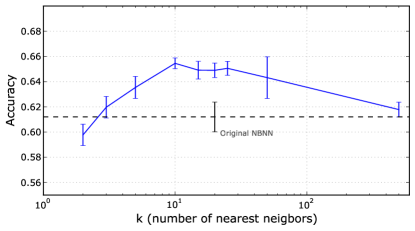
Figure 3: The effect of changing $k$, the number of nearest neighbors retrieved from the merged index. Using only the local neighbors (about 10) results in optimal performance. The absolute performance numbers are lower than in our final results because we extracted fewer SIFT descriptors for this experiment.

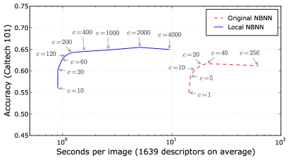
Figure 4: Comparison of accuracy against computation for NBNN vs local NBNN. Computation is determined primarily by the number of distance checks ($c$ in this figure) allowed in the approximate nearest neighbor search. For 101 classes, even a single check in each of the 101 indices is more expensive than one search with thousands of checks in the merged index due to the overhead of traversing each tree. These results were obtained on Caltech 101, using a sparser sampling of descriptors than in our final results.

Figure 4 shows the results of this experiment. There are significant improvements in both classification accuracy and computation time. Looking in each of the 101 separate class indices for just a single nearest neighbor in each, and checking only one leaf node in each of those search structures was still slower than localized search in the merged dataset. Even doing 1000, 2000, or 4000 leaf node checks in the merged dataset is still faster.

6.2 Scaling to many classes

Figure 5 further shows how the computation for these two methods grows as a function of the number of classes in the dataset. As new classes are added in our method, the depth of the randomized KD-tree search structures increases at a log rate. As we increase the number of classes to 256, local NBNN using the merged dataset runs 100 times faster than the original. In the original method, an additional search structure is required for each class, causing its linear growth rate. This requires a best-bin-first traversal of the each KD-tree. However, in the case where we query a single search structure for 10-30 nearest neighbors, the best-bin-first traversal from root to leaf happens only once, with the remainder of the nearest neighbors and distance checks being performed by backtracking. The preprocessing time to build the indices is almost identical between the two methods.

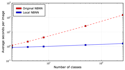
Figure 5: We varied the number of categories from 2 up to 256 and plot the run time of the two methods. When classifying 256 categories, our method is 100 times faster than the original.

6.3 Comparisons with other methods

Until now, no comparison has been done between NBNN and spatial pyramid methods using the same base feature set. We show those results in Table 2. (Runtime for the original NBNN on Caltech 256 was prohibitive, so we do not report those results.)

We choose to compare against two spatial pyramid methods. First, the original model introduced by Lazebnik et al. [14]. Second, a recent variant by Liu et al. [15] that takes advantage of local soft assignment in a manner similar to our local cut-off, and that uses max pooling [6] rather than average pooling within each spatial histogram bin. We trained a codebook of size 1024 for each of the training set regimes (Caltech 101 with 15 and 30 training images, Caltech 256 with 15 and 30 training images). Our spatial pyramid was 3 levels (1x1, 2x2, and 4x4 histogram arrangements). For classification, we trained one-vs-all SVMs using the histogram intersection kernel [14] and used a fixed regularization term for all training regimes.

We also compare against some previously published figures for NBNN. Notably, local NBNN gives the best performance of any NBNN method to date.

While local NBNN (and NBNN) performs better the original spatial pyramid model, it does not perform better than the model of Liu et al. The soft assignment avoids some of the information loss through quantization, and the discriminative training step provides an additional benefit.

The recent kernel NBNN of Tuytelaars et al. is a complimentary contribution, and we suspect that the combinations of local NBNN with the kernel NBNN would lead to even better performance. We hypothesize that this combination would lead to NBNN matching or improving upon the performance of state-of-the-art spatial pyramid methods.

There are other results using a single feature type that have higher published accuracy on these benchmarks. For example, Boureau et al. [5] show $77.1\%$ accuracy on Caltech 101 and $41.7\%$ on Caltech 256 with 30 training images, but they use a macro-feature built on top of SIFT as their base feature, so that is not directly comparable with our feature set. Combining different feature types together would also yield higher performance as shown frequently in literature [3, 19].

	Caltech 101 (15 training images)	Caltech 101 (30 training images)	Caltech 256 (15 training images)	Caltech 256 (30 training images)
Results from literature
NBNN [3]	65$\pm$1.14	70.4	30.51	37
NBNN [19]	62.7$\pm$0.5	65.5$\pm$1.0	-	-
NBNN kernel [19]	61.3$\pm$0.2	69.6$\pm$0.9	-	-
Results using our feature set
SPM (Hard-assignment, avg.-pooling)2	62.5$\pm$0.9	66.3$\pm$2.6	27.3$\pm$0.5	33.1$\pm$0.5
SPM (Local soft-assignment, max-pooling)3	68.6$\pm$0.7	76.0$\pm$0.9	33.2$\pm$0.8	39.5$\pm$0.4
NBNN (Our implementation)	63.2$\pm$0.94	70.3$\pm$0.6	-	-
Local NBNN	66.1$\pm$1.1	71.9$\pm$0.6	33.5$\pm$0.9	40.1

Table 2: Our local NBNN has consistent improvement over the original NBNN, outperforming all previously published results for NBNN using a single descriptor. We confirm NBNN outperforms the original spatial pyramid method, but is only competitive with the latest state-of-the-art variant.

• Boiman et al. did not do an experiment with 15 images on this dataset. The 30.5 is an interpolation from their plot.

• The original spatial pyramid match by Lazebnik et al. [14] (re-implementation).

• A recent variant of the spatial pyramid match from Liu et al. [15] (re-implementation).

• Our experiment using NBNN achieves $63.2\pm 0.9$ compared to $65.0\pm 1.14$ from [3]. The original implementation is not available, and we have had discussions with the authors to resolve these differences in performance. We attribute the disparity to unresolved differences in parameters of our feature extraction.

7 Conclusion

We have demonstrated that local NBNN is a superior alternative to the original NBNN, giving improved classification performance and a greater ability to scale to large numbers of object classes. Classification performance is improved by making adjustments only to the classes found in the local neighborhood comprising $k$ nearest neighbors. Additionally, it is much faster to search through a merged index for only the closest few neighbors rather than search for a descriptor’s nearest neighbor from each of the object classes.

Our comparison against spatial pyramid methods confirms previous results [3] claiming that NBNN outperforms the early spatial pyramid models. Further, while NBNN is competitive with the recent state-of-the-art variants of the spatial pyramid, additional discriminative training (as in the NBNN kernel of Tuytelaars et al. [19]) may be necessary in order to obtain similar performance.

As new recognition applications such as web search attempt to classify ever larger numbers of visual classes, we can expect the importance of scalability with respect to the number of classes to continue to grow in importance. For example, ImageNet [8] is working to obtain labelled training data for each visual concept in the English language. With very large numbers of visual categories, it becomes even more apparent that feature indexing should be used to identify only those categories that contain the most similar features rather than separately considering the presence of a feature in every known category.

References

- [1] S. Arya, D. M. Mount, N. S. Netanyahu, R. Silverman, and A. Y. Wu. An optimal algorithm for approximate nearest neighbor searching in fixed dimensions. Journal of the ACM, 45(6):891–923, Nov. 1998.
- [2] R. Behmo, P. Marcombes, A. Dalalyan, and V. Prinet. Towards optimal naive bayes nearest neighbor. In ECCV, pages 171–184, 2010.
- [3] O. Boiman, E. Shechtman, and M. Irani. In defense of nearest-neighbor based image classification. In CVPR, June 2008.
- [4] Y.-L. Boureau, F. Bach, Y. LeCun, and J. Ponce. Learning mid-level features for recognition. In CVPR, pages 2559–2566. IEEE, 2010.
- [5] Y.-L. Boureau, N. Le Roux, F. Bach, J. Ponce, and Y. LeCun. Ask the locals: multi-way local pooling for image recognition. In ICCV, 2011.
- [6] Y.-L. Boureau, J. Ponce, and Y. LeCun. A theoretical analysis of feature pooling in visual recognition. In ICML, 2010.
- [7] G. Csurka, C. Dance, L. Fan, J. Willamowski, and C. Bray. Visual categorization with bags of keypoints. In Workshop on Statistical Learning in Computer Vision, ECCV, volume 1, 2004.
- [8] J. Deng, W. Dong, R. Socher, L.-J. Li, K. Li, F.-F. Li, and L. Fei-Fei. ImageNet: A large-scale hierarchical image database. In CVPR, pages 248–255, June 2009.
- [9] P. Domingos and M. Pazzani. On the optimality of the simple Bayesian classifier under zero-one loss. Journal of Machine Learning - Special issue on learning with probabilistic representations, 29(2):103–130, 1997.
- [10] L. Fei-Fei, R. Fergus, and P. Perona. Learning generative visual models from few training examples: An incremental Bayesian approach tested on 101 object categories. In CVPR Workshop, Apr. 2004.
- [11] G. Griffin, A. Holub, and P. Perona. Caltech-256 Object Category Dataset. Technical report, California Institute of Technology, 2007.
- [12] F. Jurie and B. Triggs. Creating efficient codebooks for visual recognition. In CVPR, 2005.
- [13] C. H. Lampert, M. B. Blaschko, and T. Hofmann. Efficient subwindow search: a branch and bound framework for object localization. PAMI, 31(12):2129–42, Dec. 2009.
- [14] S. Lazebnik, C. Schmid, and J. Ponce. Beyond Bags of Features: Spatial Pyramid Matching for Recognizing Natural Scene Categories. CVPR, pages 2169–2178, 2006.
- [15] L. Liu, L. Wang, and X. Liu. In Defense of Soft-assignment Coding. In ICCV, 2011.
- [16] D. G. Lowe. Distinctive Image Features from Scale-Invariant Keypoints. IJCV, 60(2):91–110, Nov. 2004.
- [17] M. Muja and D. Lowe. Fast approximate nearest neighbors with automatic algorithm configuration. In VISSAPP, 2009.
- [18] C. Silpa-Anan and R. Hartley. Optimised KD-trees for fast image descriptor matching. In CVPR. IEEE, 2008.
- [19] T. Tuytelaars, M. Fritz, K. Saenko, and T. Darrell. The NBNN kernel. In ICCV, 2011.
- [20] J. Wang, J. Yang, K. Yu, F. Lv, T. Huang, and Y. Gong. Locality-constrained linear coding for image classification. In CVPR, pages 3360–3367. IEEE, 2010.