Relaxation in finite and isolated classical systems: an extension of Onsager’s regression hypothesis

Abstract

In order to derive the reciprocity relations, Onsager formulated a relation between thermal equilibrium fluctuations and relaxation widely known as regression hypothesis. It is shown in the present work how such relation can be extended to finite and isolated classical systems. This extension is derived from the fluctuation-dissipation theorem for the microcanonical ensemble. The results are exemplified with a nonintegrable system in order to motivate possible applications to dynamical systems and statistical mechanics of finite systems.

I Introduction

In his seminal work on the reciprocity relationsonsager1 ; *onsager2, Onsager formulated a hypothesis about the decay of thermal equilibrium fluctuations that was essential in his derivation. From this hypothesis, Onsager was able to relate the relaxation of nonequilibrium macroscopic observables, obtained from phenomenological equations, to the decay rate of equilibrium fluctuations of those quantities. Such a relation between those two apparently different phenomena is however quite expected from the point of view of the fluctuation-dissipation theorem derived callen 20 years after Onsager’s work. Indeed, since the derivation of the reciprocity relations from linear response theory, Onsager’s regression hypothesis is understood as a different but equivalent statement of the fluctuation-dissipation theorem.

On the other hand, Onsager’s reciprocity relations have already been extended to far from equilibrium conditions gallavotti1 in different contexts andrieux where nonlinear effects are taken into account. Those extensions are based on fluctuation theorems which quite often are derived from the so-called “chaotic hypothesis”gallavotti2 ; *gallavotti3. Hence the fluctuation theorems play the role of linear response theory beyond near equilibrium conditions and have been also applied to understand the nonequilibrium behavior of systems far from the thermodynamic limit jarzynski .

Onsager’s original work and its extensions mentioned above always focus on systems in contact with reservoirs. Here however we intend to study the near equilibrium behavior of isolated systems when they are finite and standard linear response theory cannot be applied. The relaxation to equilibrium of finite and almost isolated quantum systems has been studied experimentally using cold atoms weiss and has motivated several theoretical works which try to understand it and discuss the controversies related to the role played by the nonintegrability in this process rigol ; hanggi ; gogolin . For classical systems under such constraints, we show here that a simple extension of the fluctuation-dissipation theorem nielsen ; bonanca shows very clearly the importance of the dynamics in the relaxation to equilibrium within a description that is essentially Onsager’s regression hypothesis extended to this new situation. An important extension of the fluctuation-dissipation theorem for the microcanonical ensemble was first derived by Nielsen nielsen . It deals with thermodynamic responses to thermal disturbances as for example heat pulses. In Ref.bonanca , only the response to mechanical disturbances, i.e., those which can be described as additional terms in the Hamiltonian, are considered. Since they treat different aspects of the same subject, these works complement each other.

II Derivation

We start presenting the usual regression hypothesis expressed in mathematical terms. Let us consider a system described by the following Hamiltonian

$$H(\lambda_{o}+d\lambda)=H(\lambda_{o})+d\lambda\,\frac{\partial H}{\partial\lambda}\bigg{|}_{\lambda=\lambda_{o}}.$$ (1)

When the value of the parameter $\lambda$ is suddenly switched from $\lambda_{1}=\lambda_{o}+d\lambda$ to $\lambda_{o}$ at $t=t_{o}$, the nonequilibrium average value $\bar{B}$ of an observable $B$ of the system evolves as tuckerman

$$\bar{B}(t-t_{o})=\left\langle B\right\rangle_{\lambda_{o}}-\frac{d\lambda}{k_{B}T}C_{\lambda_{1}}(t-t_{o}),$$ (2)

for $t>t_{o}$, where $\langle\cdot\rangle_{\lambda_{o}}$ denotes the equilibrium average value when $\lambda=\lambda_{o}$, $k_{B}$ is the Boltzmann constant, $T$ is the temperature and

$$C_{\lambda_{1}}(t)=\langle\delta A(0)\delta B(t)\rangle_{\lambda_{1}}$$ (3)

is the correlation function with $\delta X(t)=X(t)-\langle X\rangle_{\lambda_{1}}$ and $A=(\partial H/\partial\lambda)|_{\lambda=\lambda_{o}}$.

Equation (2) is Onsager’s regression hypothesis expressed mathematically. It states that the relaxation of $\bar{B}$ to the equilibrium value is possible as long as the correlation function $C_{\lambda_{1}}(t)$ decays to zero. On the other hand, if the relaxation process can be described by some sort of phenomenological equation, one obtains the decay of $C_{\lambda_{1}}(t)$ from (2). Since Eq. (2) is derived in the usual context of the canonical ensemble, the decay of the correlation function is interpreted as a consequence of the heat bath influence.

We will now derive (2) in a different context, namely, when the system is isolated and finite, i.e. there is no heat bath and the number of degrees of freedom is such that the system is not in the thermodynamic limit. We consider first the system in equilibrium under $H(\lambda_{o}+d\lambda)$. When $t$ is equal to $t_{o}$, $\lambda_{1}$ is suddenly switched to $\lambda_{o}$. The system then relaxes to a new equilibrium state. Assuming that the system was not far from the final equilibrium state, a linear response calculation describes the relaxation process. Although the situation requires the microcanonical ensemble, the fundamental equations of linear response theory do not rely on any particular ensemble kubo . For $t>t_{o}$ the Hamiltonian is $H(\lambda_{o})$ and the situation can be stated as follows: a system, whose Hamiltonian is initially given by (1), is in equilibrium when at $t=t_{o}$ the generalized force $d\lambda$ is suddenly removed and $H(\lambda_{o}+d\lambda)\to H(\lambda_{o})$. Therefore, from linear response theory, one obtains kubo

$$\bar{B}(t-t_{o})-\langle B\rangle_{\lambda_{1}}=d\lambda\int_{-\infty}^{t}ds\,\phi_{BA}(E,t-s)\Theta(s-t_{o}),$$

(4)

where $\Theta(x)$ is the step function and $\langle B\rangle_{\lambda_{1}}$ is the following microcanonical average over the phase space points $(\mathbf{q},\mathbf{p})$

$$\langle B\rangle_{\lambda_{1}}=\int d\mathbf{q}\,d\mathbf{p}\,\rho_{\lambda_{1}}(\mathbf{q},\mathbf{p})\,B(\mathbf{q},\mathbf{p}),$$ (5)

with the distribution function $\rho_{\lambda_{1}}$ given by

$$\rho_{\lambda_{1}}(\mathbf{q},\mathbf{p})=\frac{\delta\left[E-H(\mathbf{q},\mathbf{p},\lambda_{1})\right]}{Z_{\lambda_{1}}(E)},$$ (6)

where $Z_{\lambda_{1}}(E)=\int d\mathbf{q}\,d\mathbf{p}\,\delta\left[E-H(\mathbf{q},\mathbf{p},\lambda_{1})\right]$.

The response function $\phi_{BA}(E,t-s)$ is kubo

$$\phi_{BA}(E,t-s)=\langle\left\{\delta A(s),\delta B(t)\right\}\rangle_{\lambda_{1}},$$ (7)

where $\left\{\cdot,\cdot\right\}$ is the Poisson bracket, $\delta X(t)=X(\mathbf{q}(t),\mathbf{p}(t))-\langle X\rangle_{\lambda_{1}}$, $(\mathbf{q}(t),\mathbf{p}(t))$ is the solution of Hamilton’s equations of motion for $N$ degrees of freedom, $B$ is any observable and $A=(\partial H/\partial\lambda)|_{\lambda=\lambda_{o}}$.

The fluctuation-dissipation theorem bonanca yields then

$$\tilde{F}_{BA}(z,\omega)=\frac{i}{z\omega}\tilde{\chi}_{BA}(z,\omega),$$ (8)

where

$$\tilde{\chi}_{BA}(z,\omega)=$$

$$\frac{1}{2\pi}\int_{-\infty}^{\infty}d\tau\int_{0}^{\infty}dE\,e^{-(i\omega\tau+Ez)}\left[Z_{\lambda}(E)\phi_{BA}(E,\tau)\right],$$

$$\tilde{F}_{BA}(z,\omega)=$$

$$\frac{1}{2\pi}\int_{-\infty}^{\infty}d\tau\int_{0}^{\infty}dE\,e^{-(i\omega\tau+Ez)}\left[Z_{\lambda}(E)C_{BA}(E,\tau)\right],$$

and $C_{BA}(E,\tau)$, with $\tau=t-s$, is the following correlation function

$$C_{BA}(E,t-s)=\langle\delta A(s)\delta B(t)\rangle_{\lambda},$$ (11)

which differs from (3) because of the microcanonical average.

Thus, Eq.(8) leads to

$$\phi_{BA}(E,\tau)=-\frac{1}{Z_{\lambda}(E)}\frac{\partial^{2}}{\partial\tau\partial E}\left[Z_{\lambda}(E)C_{BA}(E,\tau)\right].$$ (12)

The integral in (4) can be written as

$$\int_{-\infty}^{t}ds\,\phi_{BA}(t-s)\Theta(s-t_{o})=\int_{0}^{t-t_{o}}d\tau\,\phi_{BA}(\tau),$$ (13)

and from (12) and (13) one obtains

$$\int_{0}^{t-t_{o}}d\tau\,\phi_{BA}(\tau)=-\frac{1}{Z_{\lambda}}\frac{\partial}{\partial E}\left[Z_{\lambda}C_{BA}(\tau)\right]\bigg{|}_{0}^{t-t_{o}}$$ (14)

The dependence on $E$ was omitted for convenience.

Therefore, the relaxation of $B$ to the new equilibrium state is described by the following expression for $t>t_{o}$

$$\bar{B}(t-t_{o})=\langle B\rangle_{\lambda_{o}}-d\lambda\frac{1}{Z_{\lambda_{1}}}\frac{\partial}{\partial E}\left[Z_{\lambda_{1}}C_{BA}(t-t_{o})\right],$$ (15)

where

$$\langle B\rangle_{\lambda_{o}}=\langle B\rangle_{\lambda_{1}}+d\lambda\frac{1}{Z_{\lambda_{1}}}\frac{\partial}{\partial E}\left[Z_{\lambda_{1}}C_{BA}(0)\right],$$ (16)

since $\lim_{\tau\to\infty}C_{BA}(\tau)=0$ is assumed.

Analogously to Eq. (2), the relaxation to equilibrium of $B$ is ruled by a correlation function related to it and the relaxation rate is given in terms of the decay rate of equilibrium fluctuations. Thus, the physical contents of Eq. (15) allow us to interpret it as an extension of Onsager’s regression hypothesis to the context of finite and isolated classical systems.

Despite the analogy with (2), Eq.(15) shows that the relaxation rate of $\bar{B}$ [as well as the decay rate of $C_{BA}(E,t)$] is given only by the statistical properties of the dynamics produced by $H(\lambda_{o})$. Since the system is isolated, there is no influence of external thermal fluctuations on the decay of $C_{BA}(E,t)$ or $\bar{B}$ as in (2). Therefore, one might ask for which kind of dynamics relaxation occurs. For integrable systems, whose motion is quasiperiodic, $C_{BA}(E,t)$ would decay only for $N\to\infty$. Nevertheless, it is well known that $C_{BA}(E,t)$ decays for chaotic systems ruelle1 ; *ruelle2; gallavotti4 ; artuso . For nonintegrable systems, the complete spectrum of behaviors, from quasi-periodic to chaotic, could be approximately obtained.

In 1971, van Kampen made severe criticism of linear response theory kampen which here, in the context of isolated and finite systems, seems to be even harder to answer. However, some of the arguments in the literature kubo ; dorfman ; evans supporting standard linear response theory come from dynamical systems theory and are well suited for the present discussion. First, it is indeed possible, as mentioned above, that a finite and isolated system shows correlation functions which decay with time. In particular, if it has a statistical property called mixing ruelle1 ; *ruelle2; dorfman , it is possible to prove that such decay necessarily happens. Second, mixing is also responsible to ensure that an arbitrary smooth distribution in phase space will approach the microcanonical one for long times. Thus, although trajectories are very sensitive to small perturbations, the time evolution of distributions is rather stable. This would justify the linearization procedure leading to Eq. (4) at least for a class of systems. There should be also a constraint on time scales since the response function (12) would be ill defined for times much shorter than the inverse of the decay rate of correlations.

Figure 1: Correlation function $C_{BA}(E^{\prime},t)$ for $B=A=(q_{1}^{4}+q_{2}^{4})/4$ and $E^{\prime}=2.5$ The solid black lines were obtained numerically for $4\times 10^{5}$ initial conditions. The dashed red lines are the fitting of $\mathcal{A}^{\prime}e^{-\alpha^{\prime}t}\cos{(\omega^{\prime}t)}$. (a) $\lambda_{1}=0.1$, $\mathcal{A}^{\prime}=21.5$, $\alpha^{\prime}=0.20$ and $\omega^{\prime}=1.7$. (b) $\lambda_{1}=0.12$, $\mathcal{A}^{\prime}=14.5$, $\alpha^{\prime}=0.17$ and $\omega^{\prime}=1.8$.

Figure 2: Relaxation of $\bar{B}$ for $B=(q_{1}^{4}+q_{2}^{4})/4$ and initial energy $E=5.0$. The solid black lines were obtained numerically for $4\times 10^{5}$ initial conditions. The dashed red lines are the predictions of Eq. (15) using $C_{BA}$ obtained numerically and the scaling property. (a) $\lambda_{1}=0.1$ switched to $\lambda_{o}=0.12$ and the value of $\langle B\rangle_{\lambda_{1}}=7.54$ obtained numerically for $4\times 10^{5}$ initial conditions with $E=5.0$ and $\lambda_{1}=0.1$. (b) $\lambda_{1}=0.12$ switched to $\lambda_{o}=0.1$ and the value of $\langle B\rangle_{\lambda_{1}}=6.55$ obtained numerically for $4\times 10^{5}$ initial conditions with $E=5.0$ and $\lambda_{1}=0.12$

III Example

In order to motivate possible applications of Eq. (15) to both low-dimensional dynamical systems and statistical mechanics of finite systems, we will consider the relaxation process in a system described by the following Hamiltonian percival

$$H=\frac{p_{1}^{2}}{2}+\frac{p_{2}^{2}}{2}+\frac{q_{1}^{2}q_{2}^{2}}{2}+\lambda\frac{(q_{1}^{4}+q_{2}^{4})}{4},$$ (17)

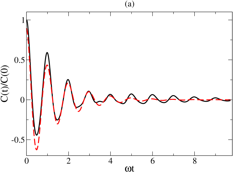
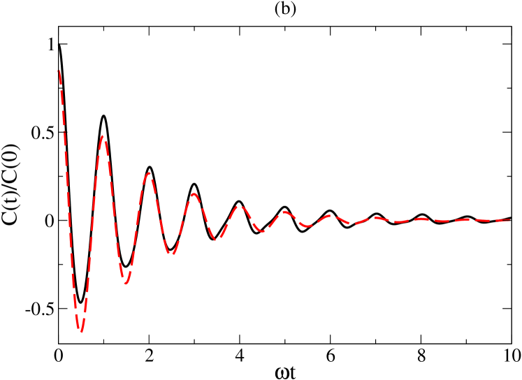
which is integrable only for $\lambda=1$. It can be verified through the Poincaré surface of sections that the motion generated by (17) gets less and less regular as $\lambda$ decreases from the value of unity. If on one hand the relaxation process is very well defined for low-dimensional hyperbolic systems, on the other hand most of the realistic models used in statistical mechanics of classical systems are nonintegrable. For a nonintegrable systems with as few degrees of freedom as (17), relaxation may or may not happen and one has to find numerically the range of parameters where it occurs. In our application of (15) to this case, we have chosen $A=(\partial H/\partial\lambda)|_{\lambda=\lambda_{o}}=(q_{1}^{4}+q_{2}^{4})/4$ and $B=A$. There is a small range of values of $\lambda$ ($0.9\lesssim\lambda\lesssim 0.13$) where $C_{BA}(\tau)$ can be fitted by the expression $\mathcal{A}e^{-\alpha\tau}\cos{(\omega\tau)}$ (see Fig.1). It is not our aim here to find the exact functional form of the correlation function. Instead we want to find out whether a simple description of it (as the one just written above) is enough to describe the relaxation process approximately.

The dynamics given by (17) is scalable with energy, i.e. the Hamilton equations remain invariant under a transformation $(q^{\prime}_{1,2},p^{\prime}_{1,2},t^{\prime})\to(q_{1,2},p_{1,2},t)$ given by the equations

$$\frac{q_{1,2}}{q^{\prime}_{1,2}}=\left(\frac{E}{E^{\prime}}\right)^{1/4},\;\frac{p_{1,2}}{p^{\prime}_{1,2}}=\left(\frac{E}{E^{\prime}}\right)^{1/4},\;\frac{t}{t^{\prime}}=\left(\frac{E^{\prime}}{E}\right)^{1/4},$$ (18)

This property of (17) yields $\mathcal{A}/\mathcal{A}^{\prime}=(E/E^{\prime})^{2}$ since $(q_{1}^{4}+q_{2}^{4})^{2}\propto(E/E^{\prime})^{2}$, $\alpha/\alpha^{\prime}=(E/E^{\prime})^{1/4}$ and $\omega/\omega^{\prime}=(E/E^{\prime})^{1/4}$. One can also verify that $Z_{\lambda}(E)\propto E^{1/2}$. Therefore, the scaling with energy allows us to perform the derivative in (15) taking a certain value $E^{\prime}$ as the reference and obtaining $C_{BA}(E,t)$ from the parameters of $C_{BA}(E^{\prime},t)$, keeping of course the same functional form and the same value of $\lambda$. In summary, the system described by (17) was chosen as an example because it allows a simple illustration of (15) applied to extremely few degrees of freedom. For models with Lennard-Jones potentials, for example, the dependence of correlation functions with energy is much more complicated and is accessible only numerically. Besides, it has been shown recently marchiori that a finite collection of (17) can act as an environment that induces relaxation on a simple degree of freedom.

IV Discussion and Conclusions

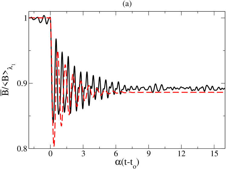
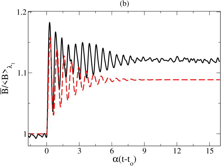
All the numerical results were obtained from the integration of the equations of motion of (17) using a fourth-order sympletic integrator forest . In Fig.1 is shown the numerical results for $C_{BA}(E^{\prime},t)$. Although it is clear that the fitting is not excellent, one obtains afterwards a good agreement between numerical and analytical results for the relaxation of $\bar{B}$. The analytical results should indeed be called semi-analytical since both $\langle B\rangle_{\lambda_{1}}$ and $C_{BA}$ were obtained numerically. In Fig.2, $\bar{B}(t-t_{o})$ is the result of the average over several $B(t-t_{o})$ obtained from the time evolution of initial conditions distributed over an energy surface with $E=5.0$. In Fig.2(a) a sudden switching of $\lambda_{1}=0.1$ to $\lambda_{o}=0.12$ at $t_{o}$ leads to the relaxation of $\bar{B}$ to a new equilibrium value. Although amplitude and frequency of oscillations are not correctly described, the relaxation time and the value of $\langle B\rangle_{\lambda_{o}}$ are well predicted. In Fig.2(b), the comparison between numerical and analytical results for $\bar{B}$ is shown for $\lambda_{1}=0.12$ switched to $\lambda_{o}=0.1$. As before, amplitude and frequency of oscillations are roughly described and the value predicted for $\langle B\rangle_{\lambda_{o}}$ is not as good as in Fig.2(a). The relaxation time however is still in good agreement with the numerical results.

In conclusion, we have derived an extension of Onsager’s regression hypothesis from linear response theory when the system of interest is isolated and finite. Although thermal fluctuations induced by a heat bath are absent in this context, the expression obtained relates, as usual, relaxation to equilibrium fluctuations. Hence the new feature is that the decay of correlations is given only by the instrinsic dynamics of the system. The relaxation of a nonintegrable systems with two degress of freedom has illustrated that. The outlook is to extend the present result to the quantum regime.