A Learning Framework for Self-Tuning Histograms

Abstract

In this paper, we consider the problem of estimating self-tuning histograms using query workloads. To this end, we propose a general learning theoretic formulation. Specifically, we use query feedback from a workload as training data to estimate a histogram with a small memory footprint that minimizes the expected error on future queries. Our formulation provides a framework in which different approaches can be studied and developed. We first study the simple class of equi-width histograms and present a learning algorithm, EquiHist, that is competitive in many settings. We also provide formal guarantees for equi-width histograms that highlight scenarios in which equi-width histograms can be expected to succeed or fail. We then go beyond equi-width histograms and present a novel learning algorithm, SpHist, for estimating general histograms. Here we use Haar wavelets to reduce the problem of learning histograms to that of learning a sparse vector. Both algorithms have multiple advantages over existing methods: 1) simple and scalable extensions to multi-dimensional data, 2) scalability with number of histogram buckets and size of query feedback, 3) natural extensions to incorporate new feedback and handle database updates. We demonstrate these advantages over the current state-of-the-art, ISOMER, through detailed experiments on real and synthetic data. In particular, we show that SpHist obtains up to $50\%$ less error than ISOMER on real-world multi-dimensional datasets.

1 Introduction

Histograms are a central component of modern databases. They are used to summarize data and estimate cardinalities of sub-expressions during query optimization. Typically, histograms are constructed solely from data and are not workload-aware. This approach has known limitations [2, 21]: First, a workload may access data non-uniformly due to which a workload-oblivious histogram might waste resources (e.g., space) on infrequently accessed parts of the data. Second, constructing a histogram from data can be expensive, requiring a scan or a sample of data; further, maintaining a histogram in the presence of updates is nontrivial. The standard approach is to rebuild histograms from scratch after a certain number of updates, resulting in possibly inaccurate histograms between builds [11].

To address these limitations, prior work has proposed self-tuning histograms [1, 2, 21]. Briefly, the idea is to collect query feedback information during query execution and to use this information to build and refine histograms. Query feedback is typically cardinalities of filter expressions over tables (e.g., $|\sigma_{5\leq A\leq 10\wedge 2\leq B\leq 3}(R)|=10$); following prior work [21] we call such cardinalities together with the corresponding query expressions as query feedback records (or QFRs). Such feedback can be collected with minimal overhead during query execution by maintaining counters at operators in the query plan [1, 15]. The overall idea is that since query feedback captures data characteristics relevant to a workload, histograms built using query feedback would be more accurate for similar workloads. Also, histograms can be refined as new feedback information is available and hence one can track changes in data characteristics arising from updates.

Over the years, several self-tuning histograms have been introduced, such as STGrid [1], STHoles [2], ISOMER [21]. Each of these methods uses an interesting way of selecting histogram bucket boundaries as well as fixing histogram bucket heights. However, most of the existing methods lack theoretical analyses/guarantees and do not scale well with high dimensions or large number of QFRs. Of particular interest is ISOMER, [21], the current state-of-the-art in self-tuning histograms. ISOMER uses query feedback to compute a “consistent” and unbiased histogram based on the maximum-entropy (maxent) principle. However, the obtained histogram might have $\Theta(N)$ buckets, given $N$ QFRs. To get a histogram with $k\ll N$ buckets, ISOMER heuristically eliminates up to $(N-k)$ feedback records. This step discards valuable feedback information and can have an adverse impact on quality, as empirically demonstrated in Section 4. Furthermore, it hinders the method’s scalability to high-dimensions or large number of QFRs. Another limitation of this approach is that it is not robust to database updates. Updates can produce inconsistent query feedback for which the maxent distribution is undefined. Again, ISOMER heuristically discards potentially useful QFRs to get a consistent subset.

In this paper, we propose and study a simple learning-theoretic formalization of self-tuning histograms. Informally, we model the QFRs as training examples drawn from some unknown distribution and the goal is to learn a $k$-bucket histogram that minimizes the expected cardinality estimation error on future queries. Our formalization is based on standard learning principles and confers several advantages: (1) Our learning algorithms leverage all available feedback information (unlike ISOMER) and in many scenarios this additional information translates to dramatic (order-of-magnitude) reductions in cardinality estimation errors (see Section 4). (2) Our framework lends itself to efficient algorithms that are scalable to multiple dimensions and large number of QFRs (3) Our formalization is database-update friendly: it is inherently robust to inconsistent QFRs and can easily incorporate natural strategies such as using higher weights for recent QFRs compared to older ones.

We next list our main algorithmic contributions:

1. Equi-width histograms: We begin by studying $1$-dimensional equi-width histograms in our learning framework and provide an efficient algorithm (EquiHist) for the same. When the number of buckets is reasonably large (relative to how spiky the true distribution is), this approach performs well in-practice. We also present a theoretical analysis that shows that the error incurred by the learned equi-width histogram is arbitrarily close to that of the best overall histogram under reasonable assumptions. This result is of independent theoretical interest; we know of no prior result that analyzes cases when equi-width histograms can be expected to succeed/fail.

2. Sparse-vector Recovery based method: One of the main contributions of this paper is a novel reduction from the general histogram learning problem to a sparse-vector recovery problem. Informally, using Haar wavelets, we represent a histogram as a sparse vector. We then cast our learning problem as that of learning a sparse-vector. To this end, we provide an efficient algorithm (SpHist) by adapting techniques from compressed sensing [22].

3. Multi-dimensional histograms: Our equi-width and sparse vector recovery algorithms admit straightforward generalizations to multi-dimensional settings. We also show that the error bounds for equi-width histograms extend to multiple dimensions. Also, SpHist admits a powerful class of histograms characterized by sparsity under Haar wavelet transformations. Using results in [24], we show that not only does this class of histograms have small memory footprint, but it can also estimate cardinality for high dimensional range queries as efficiently as existing self-tuning histograms.

4. Dynamic QFRs and Database Updates: We present online variants of our algorithms that maintain a histogram in the presence of new QFRs. We also present extensions to incorporate database updates that ensure that our learned histograms remain accurate.

Finally, we include extensive empirical evaluation of our proposed techniques over real and standard synthetic datasets, including comparisons with prior work such as ISOMER. Our empirical results demonstrate significant improvement over ISOMER in terms of accuracy in query cardinality estimation for several scenarios and databases.

Outline: We present notations and preliminaries in Section 2. We then present our equi-width as well sparse-recovery based approaches in Section 3. We provide empirical evaluation of our methods in Section 4 . In Section 5, we present some of the related works to our work and contrast them against our methods, and finally conclude with Section 6.

2 Notation and Preliminaries

In this section we introduce notation and review concepts from learning used in the paper.

For 1-dimensional histograms, $R$ and $A$ denote the relation and the column, respectively, over which a histogram is defined. We assume throughout that the domain of column $A$ is $[1,\ldots,r]$; our algorithms can be generalized to handle categorical and other numeric domains. Also, let $M$ be the number of records in $R$, i.e., $M=|R|$. A histogram over $A$ consists of $k$ buckets $B_{1},\ldots,B_{k}$. Each bucket $B_{j}$ is associated with an interval $[\ell_{j},u_{j}]$ and a count $n_{j}$ representing (an estimate of) the number of values in $R(A)$ that belong to interval $[\ell_{j},u_{j}]$. The intervals $[\ell_{j},u_{j}](1\leq j\leq k)$ are non-overlapping and partition the domain $[1,r]$. We say that the width of bucket $B_{j}$ is $(u_{j}-\ell_{j}+1)$. A histogram represents an approximate distribution of values in $R(A)$; the estimated frequency of value $i\in[\ell_{j},u_{j}]$ is $\frac{n_{j}}{u_{j}-\ell_{j}+1}$. We use interval $[\ell,u]$ to represent the range query $\sigma_{A\in[\ell,u]}(R)$.

For conciseness, we use a vector notation to represent queries and histograms. We denote vectors by lower-case bold letters (e.g. $\mathbf{\bm{w}}$) and matrices by upper-case letters (e.g., $A$). The term $w_{i}$ denotes the $i$-th component of $\mathbf{\bm{w}}$ and $\mathbf{\bm{a}}^{T}\mathbf{\bm{b}}$ (or $\mathbf{\bm{a}}\cdot\mathbf{\bm{b}}$) $=\sum_{i}a_{i}b_{i}$ denotes inner product between vectors $\mathbf{\bm{a}}$ and $\mathbf{\bm{b}}$. We represent a histogram as a vector $\mathbf{\bm{h}}\in\mathbb{R}^{r}$ specifying its estimated distribution, i.e., $h_{i}=\frac{n_{j}}{u_{j}-\ell_{j}+1}$. By definition $\mathbf{\bm{h}}$ is constant in each of $k$ bucket intervals and we refer to such vectors as $k$-piecewise constant. We represent a range query $q=[\ell,u]$ in unary form as $\mathbf{\bm{q}}\in\mathbb{R}^{r}$ where $q_{i}=1,\forall i\in[\ell,u]$ and $q_{i}=0$, otherwise. Hence, the estimated cardinality of $q$ using $\mathbf{\bm{h}}$, denoted $\hat{s}_{\mathbf{\bm{q}}}$, is given by $\hat{s}_{\mathbf{\bm{q}}}=\mathbf{\bm{q}}^{T}\mathbf{\bm{h}}.$

When discussing multi-dimensional histograms, we use $A_{1},\ldots,$ $A_{d}$ to denote the $d$ columns over which a histogram is defined. For ease of exposition, we assume all column domains are $[1,r]$. We first present notation for $d=2$: A histogram is a (estimated) value distribution over every possible assignment of values to columns $A_{1}$ and $A_{2}$, and can be represented as a matrix $H\in\mathbb{R}^{r\times r}$. A $k$-bucket histogram has $k$ non-overlapping rectangles with uniform estimated frequency within each rectangle; we also consider other kinds of “sparse” histograms that we define in Section 3.4. A query $Q$ is of the form $\sigma_{A_{1}\in[\ell_{1},u_{1}]\wedge A_{2}\in[\ell_{2},u_{2}]}(R)$ and can be represented in unary form as a matrix $Q\in\mathbb{R}^{r\times r}$. The estimated cardinality of query $Q$ using histogram $H$ is given by their inner product $\hat{s}_{Q}=\langle Q,H\rangle=Tr(Q^{T}H)$. For $d>2$, histograms and queries are $d$-dimensional tensors ($\in\mathbb{R}^{r\times\cdots\times r}$); estimated cardinality of query $Q\in\mathbb{R}^{r\times\cdots\times r}$ for histogram $H\in\mathbb{R}^{r\times\cdots\times r}$ is given by tensor inner product $\hat{s}_{Q}=\langle Q,H\rangle$.

$L_{p}$-norm: $\|\mathbf{\bm{x}}\|_{p}$ denotes $L_{p}$ norm of $\mathbf{\bm{x}}\in\mathbb{R}^{r}$ and is given by $\|\mathbf{\bm{x}}\|_{p}=(\sum_{i=1}^{r}|x_{i}|^{p})^{1/p}$.

Lipschitz Functions: A function $f:\mathbb{R}^{r}\rightarrow\mathbb{R}$ is $L$-Lipschitz continuous if: $\forall\mathbf{\bm{x}},\mathbf{\bm{y}},\ |f(\mathbf{\bm{x}})-f(\mathbf{\bm{y}})|\leq\|\mathbf{\bm{x}}-\mathbf{\bm{y}}\|_{2}\cdot L.$

Convex Functions: A function $f:\mathbb{R}^{r}\rightarrow\mathbb{R}$ is convex if:

$$\forall~{}0\leq\lambda\leq 1,\mathbf{\bm{x}},\mathbf{\bm{y}}\in\mathbb{R}^{r},\ f(\lambda\mathbf{\bm{x}}+(1-\lambda)\mathbf{\bm{y}})\leq\lambda f(\mathbf{\bm{x}})+(1-\lambda)f(\mathbf{\bm{y}}).\vspace*{-3pt}$$

Furthermore, a $f:\mathbb{R}^{r}\rightarrow\mathbb{R}$ is $\alpha$-strongly convex ($\alpha>0$) w.r.t. $L_{2}$ norm if, $\forall~{}0\leq\lambda\leq 1,\mathbf{\bm{x}},\mathbf{\bm{y}}\in\mathbb{R}^{r}$:

$$f(\lambda\mathbf{\bm{x}}+(1-\lambda)\mathbf{\bm{y}})\leq\lambda f(\mathbf{\bm{x}})+(1-\lambda)f(\mathbf{\bm{y}})-\alpha\frac{\lambda(1-\lambda)}{2}\|\mathbf{\bm{x}}-\mathbf{\bm{y}}\|_{2}^{2}.\vspace*{-3pt}$$

Let $H\in\mathbb{R}^{r\times r}$ be the Hessian of $f$, then $f$ is $\alpha$-strongly convex iff smallest eigenvalue of $H$ is greater than $\alpha$.

Empirical-risk minimization: In many learning applications, the input is a set of training examples $\mathcal{X}=\{\mathbf{\bm{x}}_{i},1\leq i\leq n\}$ and their labels/predictions $\mathbf{\bm{Y}}=\{y_{i},1\leq i\leq n\}$. The goal is to minimize expected error on unseen test points after training on a small training set $\mathcal{X}$. Empirical-risk minimization (ERM) is a canonical algorithm to provably achieve this goal for a setting given below.

Let each training sample $\mathbf{\bm{x}}_{i}$ be sampled i.i.d. from a fixed distribution $\mathcal{D}$, i.e. $\mathbf{\bm{x}}_{i}\sim\mathcal{D}$. Let $\ell(\mathbf{\bm{w}};\mathbf{\bm{x}}):\mathbb{R}^{r}\times\mathbb{R}^{r}\rightarrow\mathbb{R}$ be the loss function that provides loss incurred by model parameters $\mathbf{\bm{w}}$ for a given point $\mathbf{\bm{x}}$. Then, the goal is to minimize expected loss, i.e.,

$$\min_{\mathbf{\bm{w}}\in\mathcal{W}}F(\mathbf{\bm{w}})=\mathbb{E}_{\mathcal{D}}\left[\ell(\mathbf{\bm{w}};\mathbf{\bm{x}})\right].\vspace*{-3pt}$$ (1)

Let $\mathbf{\bm{w}}^{*}$ be the optimal solution to (1).

Typically, the distribution $\mathcal{D}$ is unknown. To address this, the empirical risk minimization (ERM)approach uses the empirical distribution derived from the training data in lieu of $\mathcal{D}$. Formally, ERM solves for:

$$\hat{\mathbf{\bm{w}}}=\min_{\mathbf{\bm{w}}\in\mathcal{W}}\hat{F}(\mathbf{\bm{w}})=\frac{1}{n}\sum_{i=1}^{n}\ell(\mathbf{\bm{w}};\mathbf{\bm{x}}_{i}).\vspace*{-3pt}$$ (2)

If loss function $\ell$ satisfies certain properties then we can prove bounds relating the quality (objective function value $F(\cdot)$) of $\hat{\mathbf{\bm{w}}}$ and $\mathbf{\bm{w}}^{*}$. In particular, [20] provided a bound on $F(\hat{\mathbf{\bm{w}}})$ for the case of strongly-convex loss functions:

Theorem 1 (Stochastic Convex Optimization [20])

Let $\ell(\mathbf{\bm{w}};\mathbf{\bm{x}})=f(\mathbf{\bm{w}}^{T}\mathbf{\bm{x}};\mathbf{\bm{x}})+h(\mathbf{\bm{w}})$, where $h:\mathbb{R}^{r}\rightarrow\mathbb{R}$ is a $\alpha$-strongly convex regularization function. Let $f(u;\mathbf{\bm{x}})$ be a convex $L_{f}$-Lipschitz continuous function in $u$ and let $\|\mathbf{\bm{x}}\|_{2}\leq R$. Let $\mathbf{\bm{w}}^{*}$ be the optimal solution of Problem (1) and $\hat{\mathbf{\bm{w}}}$ be the optimal solution of Problem (2). Then, for any distribution over $\mathbf{\bm{x}}$ and any $\delta>0$, with probability at least $1-\delta$ over a sample $\mathcal{X}$ of size $n$:

$$F(\hat{\mathbf{\bm{w}}})-F(\mathbf{\bm{w}}^{*})\leq O\left(\frac{R^{2}L_{f}^{2}\log(1/\delta)}{\alpha n}\right).\vspace*{-3pt}$$ (3)

Hence, the above theorem shows that solving ERM (i.e., Problem (2)) serves as a good “proxy” for solving the original problem (1) and also the additional expected error can be decreased linearly by increasing the number of training samples, i.e., $n$.

Haar-wavelets: Wavelets serve as a popular tool for compressing a regular signal (a vector in finite dimensions for our purposes) [14]. In particular, Haar wavelets can compress a piece-wise constant vector effectively and can therefore be used for a parsimonious representation of $k$-bucket histograms.

Haar wavelet performs a linear orthogonal transformation of a vector to obtain wavelet coefficients. In particular, given a vector $\mathbf{\bm{x}}\in\mathbb{R}^{r}$, we obtain a vector $\mathbf{\bm{\alpha}}\in\mathbb{R}^{r}$ of wavelet coefficient using:

$$\mathbf{\bm{\alpha}}=\Psi\mathbf{\bm{x}},$$ (4)

where $\Psi\in\mathbb{R}^{r\times r}$ is the wavelet transform matrix given by:

$$\Psi=\begin{cases}\frac{1}{\sqrt{r}}&\text{ if }i=1,0<j\leq r,\\ +\sqrt{\frac{2^{\left\lceil\log_{2}i\right\rceil}}{r}}&\text{ if }1<i\leq r,\frac{r}{2^{\left\lceil\log_{2}i\right\rceil}}(i-2^{\left\lceil\log_{2}i\right\rceil})<j\\ &\qquad\qquad\leq\frac{r}{2^{\left\lceil\log_{2}i\right\rceil}}(i+\frac{1}{2}-2^{\left\lceil\log_{2}i\right\rceil}),\\ -\sqrt{\frac{2^{\left\lceil\log_{2}i\right\rceil}}{r}}&\text{ if }1<i\leq r,\frac{r}{2^{\left\lceil\log_{2}i\right\rceil}}(i+\frac{1}{2}-2^{\left\lceil\log_{2}i\right\rceil})<j\\ &\qquad\qquad\leq\frac{r}{2^{\left\lceil\log_{2}i\right\rceil}}(i+1-2^{\left\lceil\log_{2}i\right\rceil}),\\ 0&\text{ otherwise. }\end{cases}$$ (5)

We can show that if $\mathbf{\bm{x}}$ is $k$-piecewise constant in Equation 4, $\mathbf{\bm{\alpha}}$ has at most $k\log r$ non-zero coefficients.

For signals in higher dimensions, wavelet transform can be obtained by first vectorizing the signal and then applying the transformation of Equation 4 (see [14] for more details). Several existing studies show that high-dimensional real-life data mostly resides in a small number of clusters and hence most of the wavelet coefficients are nearly zero [7], i.e., vector of coefficients is sparse.

3 Method

In this section, we present our learning theoretic framework and algorithms. We first review the architectural context for self-tuning histogram learning.

Architecture: We assume the architectural context of prior work in self-tuning histograms [21]. In particular, we assume operators in query plans are instrumented to maintain counters and produce query feedback records (QFRs) at the end of query execution. Recall that a QFR is a filter sub-expression and its cardinality. (In the following, we abuse notation and refer to such sub-expressions as queries although they are actually parts of a query.) These QFRs are available as input to our learning system either continuously or in a batched fashion (e.g., during periods of low system load). Although we present our learning framework assuming QFRs are the only input, we can extend our framework to incorporate workload-independent data characteristics, e.g., an initial histogram constructed from data.

First, in Section 3.1, we present our learning theoretic framework for self-tuning histograms. In Section 3.2 we study equi-width histograms in our framework and present a learning algorithm for the same (EquiHist). We also present formal error analysis for histograms learned by EquiHist. Equi-width histograms are known to be unsuitable in many settings, such as sparse high-dimensional datasets. To handle this, in Section 3.3, we present an algorithm (SpHist) for learning general histograms that relies on a reduction from histogram learning to sparse vector recovery. For presentational simplicity, Sections 3.1-3.3 assume static QFRs, no database updates, and 1-dimensional histograms. We extend our algorithms to multidimensional histograms in Section 3.4 and dynamic data and QFRs in Section 3.5.

3.1 Problem Formulation

We now formalize the histogram estimation problem. Our formulation is based on standard learning assumptions where we assume a training query workload of QFRs which is sampled from a fixed distribution and the goal is to estimate a $k$-bucket histogram that incurs small expected error for unseen queries from the same distribution. We consider histograms over column $A$ of relation $R$. Recall from Section 2 that domain of $A$ is $[1,r]$ and a $k$-bucket histogram $\mathbf{\bm{h}}\in\mathbb{R}^{r}$ is a $k$-piecewise constant vector.

Let $\mathcal{D}$ be a fixed (unknown) distribution of range queries over $R(A)$. Let $\mathcal{Q}=\{(\mathbf{\bm{q}}_{1},s_{\mathbf{\bm{q}}_{1}}),\dots,(\mathbf{\bm{q}}_{N},s_{\mathbf{\bm{q}}_{N}})\}$ be a query workload used for training where each $\mathbf{\bm{q}}_{i}\sim\mathcal{D},\forall 1\leq i\leq N$ and $s_{\mathbf{\bm{q}}}$ is the cardinality of query $\mathbf{\bm{q}}$ when evaluated over $R$.

Let $f(\hat{s}_{\mathbf{\bm{q}}};s_{\mathbf{\bm{q}}}):\mathbb{R}\times\mathbb{R}\rightarrow\mathbb{R}$ be a loss function that measures the error between the estimated cardinality, $\hat{s}_{\mathbf{\bm{q}}}$, and actual cardinality, $s_{\mathbf{\bm{q}}}$, of query $\mathbf{\bm{q}}$. Since the estimated cardinality of $\mathbf{\bm{q}}$ using histogram $\mathbf{\bm{h}}$ is $\hat{s}_{\mathbf{\bm{q}}}=\mathbf{\bm{q}}^{T}\mathbf{\bm{h}}$, the error incurred by $\mathbf{\bm{h}}$ on $\mathbf{\bm{q}}$ is $f(\mathbf{\bm{q}}^{T}\mathbf{\bm{h}};s_{\mathbf{\bm{q}}})$. Example loss functions include $L_{1}$ loss ($f(\mathbf{\bm{q}}^{T}\mathbf{\bm{h}};s_{\mathbf{\bm{q}}})=|\mathbf{\bm{q}}^{T}\mathbf{\bm{h}}-s_{\mathbf{\bm{q}}}|$) and $L_{2}$ loss ($f(\mathbf{\bm{q}}^{T}\mathbf{\bm{h}};s_{\mathbf{\bm{q}}})=(\mathbf{\bm{q}}^{T}\mathbf{\bm{h}}-s_{\mathbf{\bm{q}}})^{2}$).

Our goal is to learn a $k$-bucket histogram $\mathbf{\bm{h}}\in\mathbb{R}^{r}$ that minimizes the expected error $F(\mathbf{\bm{h}})=\mathbb{E}_{\mathbf{\bm{q}}\sim\mathcal{D}}[f(\mathbf{\bm{q}}^{T}\mathbf{\bm{h}};s_{\mathbf{\bm{q}}})]$ incurred by $\mathbf{\bm{h}}$ on test queries sampled from $\mathcal{D}$. Formally, we define our histogram estimation problem as:

$$\min_{\mathbf{\bm{h}}}\ \ F_{\mathcal{D}}(\mathbf{\bm{h}}),\quad\text{s.t.}\ \ \mathbf{\bm{h}}\in\mathcal{C},$$ (6)

and let $\mathbf{\bm{h}}^{*}$ be the optimal solution to the above problem, i.e.,

$$\mathbf{\bm{h}}^{*}=\mathop{\mathrm{argmin}}_{\mathbf{\bm{h}}\in\mathcal{C}}F_{\mathcal{D}}(\mathbf{\bm{h}}),$$ (7)

where $\mathcal{C}$ represents the following set of histograms:

$$\mathcal{C}=\{\mathbf{\bm{h}}\>:\> \mathbf{\bm{h}}\in\mathbb{R}^{r}\text{ is a histogram over range }[1,r]\text{with}$$

$$\text{at most }k\text{ buckets and minimum bucket-width }\Delta\}$$ (8)

Note that $\mathcal{C}$ only contains histograms whose each bucket is of width at least $\Delta$. Parameter $\Delta$ can be arbitrary; we introduce it for the purpose of analysis only. While our analysis do not make any assumption on $\Delta$, naturally, bounds would be better if $\Delta$ of the optimal histogram is large, i.e., the optimal histogram is relatively flat.

We next study equi-width histograms in our framework and provide an efficient algorithm for the same.

3.2 Equi-width Approach

In this section, we study equi-width histograms for solving Problem (6) and also provide approximation guarantees for the obtained method.

Observe that set $\mathcal{C}$ (Equation 8) is a non-convex set, hence we cannot apply standard convex optimization techniques to obtain the optimal solution to (6). To handle this, we relax the problem by fixing the bucket boundaries to be equi-spaced. That is, we first consider the class of histograms with $b$ equal-width buckets:

$$\mathcal{C}^{\prime}=\{\mathbf{\bm{h}}\>:\> \mathbf{\bm{h}}\in\mathbb{R}^{r}\text{ is a histogram over integer range }[1,r]$$

$$\text{with }b\text{ equal-width buckets}\}.$$ (9)

For ease of exposition, we assume $r$ is divisible by $b$. Note that, for any $\mathbf{\bm{h}}\in\mathcal{C}^{\prime}$, we can find $\mathbf{\bm{w}}\in\mathbb{R}^{b}$ such that $\mathbf{\bm{h}}=B\mathbf{\bm{w}}$, where $B\in\mathbb{R}^{r\times b}$ and

$$B_{ij}=\begin{cases}1&\text{ if }\frac{r}{b}\cdot(j-1)<i\leq\frac{r}{b}\cdot j,\\ 0&\text{otherwise}.\end{cases}$$ (10)

For illustration (with $\frac{r}{b}=2$),

$$\mathbf{\bm{h}}=\left[\begin{array}[]{c}w_{1}\\ w_{1}\\ w_{2}\\ w_{2}\\ \vdots\end{array}\right]=\left[\begin{array}[]{ccc}1&0&\cdots\\ 1&0&\cdots\\ 0&1&\cdots\\ 0&1&\cdots\\ \vdots&\vdots&\vdots\end{array}\right]\cdot\left[\begin{array}[]{c}w_{1}\\ w_{2}\\ \vdots\end{array}\right].$$ (11)

Therefore, searching for a histogram $\mathbf{\bm{h}}$ over $\mathcal{C}^{\prime}$ is equivalent to searching for a $\mathbf{\bm{w}}\in\mathbb{R}^{b}$. Furthermore, optimal $\mathbf{\bm{h}}^{*}$ to (6) should satisfy: $\|\mathbf{\bm{h}}^{*}\|_{1}=\sum_{i}h_{i}=M$, i.e., total number of database records. Also, $\mathbf{\bm{h}}^{*}$ should have minimum bucket width $\Delta$, hence $\|\mathbf{\bm{h}}^{*}\|_{\infty}\leq\frac{M}{\Delta}$. Using these observations, we can constraint $\mathbf{\bm{w}}$ to belong to a convex set $\mathcal{K}$:

$$\mathcal{K}=\{\mathbf{\bm{w}}\in\mathbb{R}^{b}|\ \|\mathbf{\bm{w}}\|_{1}=\frac{Mb}{r}\text{ and }\|\mathbf{\bm{w}}\|_{\infty}\leq\frac{M}{\Delta}\}.$$ (12)

Thus, $\mathcal{C}^{\prime}$ can be redefined as:

$$\mathcal{C}^{\prime}=\{\mathbf{\bm{h}}\>:\>\mathbf{\bm{h}}=B\mathbf{\bm{w}},\mathbf{\bm{w}}\in\mathcal{K}\},$$ (13)

and searching for a histogram $\mathbf{\bm{h}}$ over $\mathcal{C}^{\prime}$ induces a corresponding search for $\mathbf{\bm{w}}$ over $\mathcal{K}$, which is a convex set.

Using the above observations, we obtain the following relaxed problem:

$$\min_{\mathbf{\bm{w}}\in\mathcal{K}}F_{\mathcal{D}}(B\mathbf{\bm{w}}).$$ (14)

To avoid overfitting, we add entropy regularization to the above objective function. This leads to the following relaxed problem:

$$\min_{\mathbf{\bm{w}}\in\mathcal{K}}G_{\mathcal{D}}(\mathbf{\bm{w}})=E_{\mathcal{D}}\left[f(\mathbf{\bm{q}}^{T}B\mathbf{\bm{w}};s_{\mathbf{\bm{q}}})\right]-\lambda H(\frac{r}{Mb}\mathbf{\bm{w}}),$$ (15)

where $M$ is the size of the relation $R$, i.e., $M=|R|$, $\lambda>0$ is a constant specified later and $H(\frac{r}{Mb}\mathbf{\bm{w}})=-\sum_{j=1}^{b}\frac{w_{i}r}{Mb}$ $\times\log\frac{w_{i}r}{Mb}$ is the entropy of $\frac{r}{Mb}\mathbf{\bm{w}}$. Note that we normalized each $w_{i}$ by multiplying by $r/(Mb)$ to make it a probability distribution.

The distribution $\mathcal{D}$ is unknown except through the example queries in $\mathcal{Q}$, and so we cannot directly solve (15). As mentioned in Section 2, we instead optimize an empirical estimate ($\hat{G}(\cdot)$) of the objective $G_{\mathcal{D}}(\cdot)$, which finally leads us to the following problem:

$$\min_{\mathbf{\bm{w}}\in\mathcal{K}}\hat{G}(\mathbf{\bm{w}})=\frac{1}{N}\sum_{i=1}^{N}f(\mathbf{\bm{q}}_{i}^{T}B\mathbf{\bm{w}};s_{\mathbf{\bm{q}}_{i}})-\lambda H(\frac{r}{Mb}\mathbf{\bm{w}}),$$ (16)

where $\mathcal{K}$ is given by (12). Let $\hat{\mathbf{\bm{w}}}$ be the optimal solution to (16), i.e.,

$$\hat{\mathbf{\bm{w}}}=\mathop{\mathrm{argmin}}_{\mathbf{\bm{w}}\in\mathcal{K}}\hat{G}(\mathbf{\bm{w}}),\quad\hat{\mathbf{\bm{h}}}=B\hat{\mathbf{\bm{w}}}.$$

Now note that the above relaxed problem is a convex program and can be solved optimally and efficiently using standard convex optimization methods. However, the obtained solution need not be optimal for our original problem (6).

Interestingly, in the following theorem, we show that optimal equi-width histogram $\hat{\mathbf{\bm{h}}}\in\mathcal{C}^{\prime}$ is a provably approximate solution to the original problem (6). In particular, the theorem shows that by training with a finite number of queries ($N$) and selecting number of buckets $b$ to be a multiplicative factor larger than the required number of buckets $k$, the objective function (in Problem 6) at $\hat{\mathbf{\bm{h}}}$ is at most $\epsilon$ larger than the optimal value.

Theorem 2

Let $f:\mathbb{R}\times\mathbb{R}\rightarrow\mathbb{R}$ be a convex $L_{f}$-Lipschitz continuous loss function. Let $\hat{\mathbf{\bm{w}}}$ be the optimal solution to (16), $\hat{\mathbf{\bm{h}}}=B\hat{\mathbf{\bm{w}}}$ and let each query $\mathbf{\bm{q}}_{i}\sim\mathcal{D}$. Let $\mathbf{\bm{h}}^{*}$ be the optimal solution to (6) and has minimum bucket width $\Delta$. Let $|Q|=\max_{\mathbf{\bm{q}}\sim\mathcal{D}}\|\mathbf{\bm{q}}\|_{1}$, i.e., the largest range of any query and let $C_{1},C_{2}>0$ be universal constants. Then, if the number of training queries ($N$) satisfies:

$$N\geq C_{1}\left(\frac{|Q|}{\Delta}\right)^{3}\frac{L_{f}^{4}\log\frac{1}{\delta}}{\epsilon^{4}},$$

and if the number of buckets ($b$) in $\hat{\mathbf{\bm{h}}}$ satisfies: $b\geq C_{2}k\frac{|Q|L_{f}^{2}}{\Delta\epsilon^{2}},$ we have

$$F_{\mathcal{D}}(\hat{\mathbf{\bm{h}}})=\mathbb{E}_{\mathcal{D}}[f(\mathbf{\bm{q}}^{T}\hat{\mathbf{\bm{h}}};s_{\mathbf{\bm{q}}})]\leq F(\mathbf{\bm{h}}^{*})+M\epsilon.$$

See Appendix A.1 of our full-version [23] for a detailed proof.

Note that the above theorem shows that the histogram $\hat{\mathbf{\bm{h}}}$ that we learn satisfy both the required properties:

•  Number of buckets ($b$) in $\hat{\mathbf{\bm{h}}}$ is given by $b=C_{2}k\frac{|Q|L_{f}^{2}}{\Delta\epsilon^{2}}$. Hence, number of buckets in $\hat{\mathbf{\bm{h}}}$ are larger than $k$ by a small approximation factor. In fact if queries are generally “short”, i.e., $|Q|$ is smaller than $\Delta$, then the approximation factor is a constant dependent only on the accuracy parameter $\epsilon$.

•  Relative Expected Error incurred by $\hat{\mathbf{\bm{h}}}$ is only $\epsilon$, while sampling $N=C_{1}\left(\frac{|Q|}{\Delta}\right)^{3}\frac{L_{f}^{4}\log\frac{1}{\delta}}{\epsilon^{4}}$ queries. Note that our bound on $N$ is independent of $r$, hence the number of queries is not dependent on the range of the space, but only on the “complexity” of histograms and queries considered, i.e., on $\Delta$ and $|Q|$. Our bound confirms the intuition that if $\Delta$ is smaller, that is, the optimal histograms have more buckets and is more “spiky”, then the number of queries needed is also very large. However, if $\Delta$ is a constant factor of range $r$, then the number of queries required is a constant.

Now, the above bounds depend critically upon the loss function $f$ through its Lipschitz constant $L_{f}$. In the following corollary, we provide bounds for loss function $f(\mathbf{\bm{q}}^{T}\mathbf{\bm{h}};s_{\mathbf{\bm{q}}})=|\mathbf{\bm{q}}^{T}\mathbf{\bm{h}}-s_{\mathbf{\bm{q}}}|$.

Corollary 3

Let $f(\mathbf{\bm{q}}^{T}\mathbf{\bm{h}};s_{\mathbf{\bm{q}}})=|\mathbf{\bm{q}}^{T}\mathbf{\bm{h}}-s_{\mathbf{\bm{q}}}|$, then under the assumptions of Theorem 2 and by select $N,b$ to be:

$$N\geq C_{1}\left(\frac{|Q|}{\Delta}\right)^{3}\frac{\log\frac{1}{\delta}}{\epsilon^{4}},\ \ ,b\geq C_{2}k\frac{|Q|}{\Delta\epsilon^{2}}.$$

Then,

$$F_{\mathcal{D}}(\hat{\mathbf{\bm{h}}})=\mathbb{E}_{\mathcal{D}}[|\mathbf{\bm{q}}^{T}\hat{\mathbf{\bm{h}}}-s_{\mathbf{\bm{q}}}|]\leq F(\mathbf{\bm{h}}^{*})+M\epsilon.$$

Note that $f(\mathbf{\bm{q}}^{T}\mathbf{\bm{h}};s_{\mathbf{\bm{q}}})=|\mathbf{\bm{q}}^{T}\mathbf{\bm{h}}-s_{\mathbf{\bm{q}}}|$ is $1$-Lipschitz convex function. The above corollary now follows directly from Theorem 2.
EquiHist Method: While selecting the loss function to be $L_{1}$ loss ($f(\mathbf{\bm{q}}^{T}\mathbf{\bm{h}};s_{\mathbf{\bm{q}}})=|\mathbf{\bm{q}}^{T}\mathbf{\bm{h}}-s_{\mathbf{\bm{q}}}|$) provides tight bounds, in practice optimization with $L_{1}$ loss is expensive as it is not a smooth differentiable function. Instead, for our implementation, we use $L_{2}$ loss and select regularization parameter $\lambda=0$. Hence, the empirical risk minimization problem that our Equi-width Histogram method (EquiHist) solves is given by:

$$\hat{G}(\mathbf{\bm{w}})=\min_{\mathbf{\bm{w}}\in\mathbb{R}^{b}}\frac{1}{N}\sum_{i=1}^{N}(\mathbf{\bm{q}}_{i}^{T}B\mathbf{\bm{w}}-s_{\mathbf{\bm{q}}_{i}})^{2}.$$ (17)

Using techniques similar to Theorem 2, we can easily obtain approximation guarantees for the optima of the above problem. Also, the above optimization problem is the well-known Least-squares problem and its solution can be obtained in closed form. Algorithm 1 provides a pseudo-code of our method (EquiHist). Here, $\mathcal{Q}$ is a matrix whose each row contains the training query $\mathbf{\bm{q}}_{i}$ and $s$ is the column vector containing corresponding query cardinalities.

Algorithm 1 EquiHist: Equi-width histogram based method for Histogram Estimation (1-dimensional case)

1:  Input: Training Queries: $\mathcal{Q}\in\mathbb{R}^{r\times N}$ where $i$-th column $\mathcal{Q}_{i}\in\mathbb{R}^{r}$ is the $i$-th query $\mathbf{\bm{q}}_{i}$. $\mathbf{\bm{s}}=[s_{\mathbf{\bm{q}}_{1}};s_{\mathbf{\bm{q}}_{2}};\dots;s_{\mathbf{\bm{q}}_{N}}]\in\mathbb{R}^{N}$ is the column vector of training query cardinalities

2:  Parameters: $k$: number of histogram buckets

3:  $B\in\mathbb{R}^{r\times k}$ is as given (10) (with $b=k$).

4:  $\mathbf{\bm{w}}\leftarrow(B^{T}\mathcal{Q}\mathcal{Q}^{T}B)^{-1}B^{T}\mathcal{Q}\mathbf{\bm{s}}$ (solution to (17))

5:  $\mathbf{\bm{h}}=B\mathbf{\bm{w}}$

6:  Output: $\mathbf{\bm{h}}$

3.3 Sparse-vector Recovery based Approach

In the previous subsection, we provided an approximation algorithm for Problem 6, by fixing bucket boundaries to be equi-width. However, when the number of buckets required is extremely small then selecting large equi-width buckets might incur heavy error in practice. Furthermore, in high-dimensions the histograms can be very “spiky”, hence minimum bucket width $\Delta$ might be small, leading to poor accuracies both theoretically as well in practice.

To alleviate the above mentioned problem, we formulate a sparse-vector recovery based method that is able to use recently developed methods from sparse vector recovery domain. For this purpose, we use the $L_{2}$ loss for our objective function:

$$\hat{F}(\mathbf{\bm{h}})=\frac{1}{N}\sum_{i=1}^{N}(s_{\mathbf{\bm{q}}_{i}}-\mathbf{\bm{q}}_{i}^{T}\mathbf{\bm{h}})^{2}.$$ (18)

Now, we use wavelet basis to transform $\mathbf{\bm{h}}$ into its wavelet coefficients. Let $\Psi$ be the Haar wavelet basis, and $\mathbf{\bm{\alpha}}=\Psi\mathbf{\bm{h}}$ be the wavelet transform of $\mathbf{\bm{h}}$. Since $\Psi$ is orthonormal, we can rewrite cardinality estimation using $\mathbf{\bm{h}}$ as:

$$\mathbf{\bm{q}}^{T}\mathbf{\bm{h}}=\mathbf{\bm{q}}^{T}\Psi^{T}\Psi\mathbf{\bm{h}}=\mathbf{\bm{q}}^{T}\Psi^{T}\mathbf{\bm{\alpha}},$$ (19)

where $\mathbf{\bm{\alpha}}$ is the vector of Haar wavelet coefficients of $\mathbf{\bm{h}}$. Furthermore, using standard results in wavelet transforms [14], if $\mathbf{\bm{h}}$ is $k$-piecewise constant then the wavelet transform has at most $k\log r$ non-zero coefficients. As $k$ is significantly smaller than $R$, hence wavelet transform of $\mathbf{\bm{h}}$ should be sparse and we can use sparse-vector recovery techniques from compressed sensing community to recover these wavelet coefficients.

We now describe our sparse-vector recovery based approach to estimate histograms. Below, we formally specify our sparse-wavelet coefficient recovery problem:

$$\mathbf{\bm{\alpha}}^{*}=\mathop{\mathrm{argmin}}_{\text{supp}(\mathbf{\bm{\alpha}})\leq k}\frac{1}{N}\sum_{i=1}^{N}(s_{\mathbf{\bm{q}}_{i}}-\mathbf{\bm{q}}_{i}^{T}\Psi^{T}\mathbf{\bm{\alpha}})^{2},$$ (20)

where $\text{supp}(\mathbf{\bm{\alpha}})$ is the number of non-zeros in $\mathbf{\bm{\alpha}}$.

Note that the above problem is in general NP-hard. However, several recent work in the area of compressed sensing [5, 4] show that under certain settings $\mathbf{\bm{\alpha}}^{*}$ can be obtained up to an approximation factor. Unfortunately, random range queries do not satisfy necessary conditions for sparse-vector recovery and hence formal guarantees for this approach do not follow directly from existing proof techniques. We leave proof of our approach as future work.

Instead, we use sparse-recovery algorithms as heuristics for our problem. In particular, we use one of the most popular sparse-recovery algorithm, Orthogonal Matching Pursuit (OMP) [22]. OMP is a greedy technique that starts with an empty set of coefficients (i.e. $\text{supp}(\mathbf{\bm{\alpha}})=0$). Now, at each step OMP adds a coefficient to the support set which leads to largest decrease in the objective function value. After greedily selecting $k$ coefficients, we obtain $\mathbf{\bm{\alpha}}$ and its support set with at most $k$ coefficients.

Let, $\hat{\mathbf{\bm{\alpha}}}$ be computed using OMP method, then we obtain our estimated histogram $\hat{\mathbf{\bm{h}}}$ using:

$$\hat{\mathbf{\bm{h}}}=\Psi^{T}\hat{\mathbf{\bm{\alpha}}}.$$

Note that, if $\hat{\mathbf{\bm{\alpha}}}$ has $k$ non-zeros then $\hat{\mathbf{\bm{h}}}$ will have at most $3k$ non-zeros [16], hence our estimated histogram has small number of buckets. To further decrease the number of buckets to $k$, we use the dynamic programming based method by [12] that produces small number of buckets if heights (or probability density value) for each attribute value is provided. Also, the method of [12] runs in time quadratic in the number of attribute values, i.e., range $r$. However, since our frequency distribution (histogram $\hat{\mathbf{\bm{h}}}$) has only $3k$ buckets, we can modify the Dynamic Programming based algorithm of [12] so that it obtains the optimal solution in time $O(k^{2})$. Algorithm 2 provides a pseudo-code of our algorithm. $\mathcal{Q}$ denotes training queries matrix and $A_{\mathcal{S}}\in\mathbb{R}^{N\times|{\mathcal{S}}|}$ represents a sub-matrix of $A$ formed by $A$’s columns indexed by ${\mathcal{S}}$.

Algorithm 2 SpHist: Sparse-recovery based Histogram Estimation (1-dimensional case)

1:  Input: Training Queries: $\mathcal{Q}\in\mathbb{R}^{r\times N}$ where $i$-th column $\mathcal{Q}_{i}\in\mathbb{R}^{r}$ is the $i$-th query $\mathbf{\bm{q}}_{i}$. $\mathbf{\bm{s}}=[s_{q_{1}};s_{q_{2}};\dots;s_{q_{N}}]\in\mathbb{R}^{N}$ is the column vector of training query cardinalities

2:  Parameters: $k$: number of histogram buckets

3:  Set support set ${\mathcal{S}}=\phi$, residual $\mathbf{\bm{z}}_{0}=\mathbf{\bm{s}}$.

4:  Set $A=\mathcal{Q}^{T}\Psi^{T}$ (note that $A\in\mathbb{R}^{N\times r}$)

5:  $t=1$

6:  repeat

7:     Find index $I_{t}=\mathop{\mathrm{argmax}}_{j=1,...,r}\mathbf{\bm{z}}_{t-1}^{T}A_{j}$

8:     ${\mathcal{S}}={\mathcal{S}}\cup\{I_{t}\}$

9:     $\mathbf{\bm{\alpha}}^{t}=\bm{0}$ ($\mathbf{\bm{\alpha}}^{t}\in\mathbb{R}^{r}$)

10:     Least Squares Solution: $\mathbf{\bm{\alpha}}^{t}_{\mathcal{S}}=\mathop{\mathrm{argmin}}_{\mathbf{\bm{\alpha}}_{\mathcal{S}}\in\mathbb{R}^{|{\mathcal{S}}|}}\|A_{\mathcal{S}}\mathbf{\bm{\alpha}}_{\mathcal{S}}-\mathbf{\bm{s}}\|_{2}$. $//$ $A_{\mathcal{S}}$ is the column submatrix of $A$ whose columns are listed in ${\mathcal{S}}$. $\mathbf{\bm{\alpha}}^{t}_{\mathcal{S}}$ is the sub-vector of $\mathbf{\bm{\alpha}}^{t}$ with components listed in set ${\mathcal{S}}$.

11:     Update residual: $\mathbf{\bm{z}}_{t}=\mathbf{\bm{s}}-A\mathbf{\bm{\alpha}}^{t}$.

12:     $t=t+1$

13:  until ($t\leq k$)

14:  $\hat{\mathbf{\bm{\alpha}}}=\mathbf{\bm{\alpha}}^{k}$

15:  Form $\hat{\mathbf{\bm{h}}}=\Psi^{T}\hat{\mathbf{\bm{\alpha}}}$

16:  Apply modified version of DP Method of [12] to $\hat{\mathbf{\bm{h}}}$ to obtain $\mathbf{\bm{h}}$ with $k$ buckets

17:  Output: Histogram $\mathbf{\bm{h}}$ with $k$ buckets

3.4 Multi-dimensional Histograms

In the previous two subsections, we discussed our two approaches for $1$-dimensional case. In this section, we extend both the approaches for multi-dimensional case as well. In next subsection we discuss EquiHist generalization to multiple dimensions and in Subsection 3.4.2, we generalize our sparse recovery based approach.

3.4.1 Equi-width Approach

We first provide an extension of the equi-width approach to the 2-d case and then briefly discuss extensions to general multi-dimensional case.

Recall that, given a set of range queries $\mathcal{Q}=\{Q_{1},\dots,Q_{N}\}$ and their cardinality $\mathbf{\bm{s}}=\{s_{Q_{1}},s_{Q_{2}},\dots,s_{Q_{n}}\}$ where $Q_{i}\in\mathbb{R}^{r\times r}$ and $Q_{i}\sim\mathcal{D}$, the goal is to learn histogram $H\in\mathbb{R}^{r\times r}$ such that $H$ has at most $k$ buckets. For 2-D case, we consider a bucket to be a rectangle only. Note that $H$ can have arbitrary rectangular buckets, hence the class of $H$ considered is more general than STGrid. But, our class of $H$ is restricted compared to STHoles, which has an extra “universal” bucket. Now, as for the $1$-d case, the goal is to minimize expected error in cardinality estimation, i.e.,

$$\min_{H\in\mathcal{C}}E_{\mathcal{D}}\left[f(\langle Q,H\rangle;s_{Q})\right],$$ (21)

where $\langle Q,H\rangle=Tr(Q^{T}H)$ denotes the inner product between $Q$ and $H$, and $\mathcal{C}$ is given by:

$$\mathcal{C}=\{H\in\mathbb{R}^{r\times r}:\text{ H has }k\text{ rectangular buckets }\\ \text{ and minimum bucket size }\Delta\times\Delta\}$$ (22)

Similar to $1$-d case, we restrict histograms to set $\mathcal{C}^{\prime}$ that consists of $b=b_{1}\times b_{1}$ equi-width buckets. Now it is easy to verify that for any $H\in\mathcal{C}^{\prime}$, we can find a matrix $W\in\mathbb{R}^{b_{1}\times b_{1}}$ s.t.,

$$H=BWB^{T},$$ (23)

where $B\in\mathbb{R}^{r\times b_{1}}$ is as defined in (10).

Hence, $\mathcal{C}^{\prime}$ can be defined as:

$$\mathcal{C}^{\prime}=\{H:H=BWB^{T},W\in\mathcal{K}\},$$ (24)

where $\mathcal{K}$ is a convex set defined analogously to (12).

Selecting entropy regularization and using empirical estimate for optimization, we reduce (21) to the following problem:

$$\min_{W\in\mathcal{K}}\hat{G}(W)=\frac{1}{N}\sum_{i=1}^{N}f(\langle Q,BWB^{T}\rangle;s_{Q})-\lambda H\left(\frac{r\cdot r}{Mb}W\right),$$ (25)

where $M=|R|$, i.e. relation cardinality and $\lambda>0$ is a constant.

Let $\hat{W}$ be the optimal solution to the above problem and let $\hat{H}=B\hat{W}B^{T}$. Now, similar to 1-D case, we bound the expected error incurred by $\hat{H}$ when compared to the optimal histogram $H^{*}\in\mathcal{C}$ to Problem 21.

Theorem 4

Let $f:\mathbb{R}\times\mathbb{R}\rightarrow\mathbb{R}$ be a convex $L_{f}$-Lipschitz continuous loss function. Let $\hat{W}=\mathop{\mathrm{argmin}}_{W\in\mathcal{K}}\hat{G}(W)$ and $\hat{H}=B\hat{W}B^{T}$ and each $Q_{i}\sim\mathcal{D}$. Let $\mathcal{K}\subset\mathbb{R}^{b_{1}\times b_{1}}$ be a convex set; if each $W\in\mathcal{K}$ is treated as a $b_{1}\times b_{1}=b$-dimensional vector, then $\mathcal{K}$ is selected to be the intersection of the $L_{1}$ ball of radius $\frac{Mb}{r}$ and $L_{\infty}$ ball of radius $\frac{M}{\Delta}$. If we are given that

$$N\geq\left(\frac{|Q|}{\Delta}\right)^{3}\frac{L_{f}^{4}\log\frac{1}{\delta}}{\epsilon^{4}},\ \ \ b\geq k^{2}\frac{|Q|^{2}L_{f}^{2}}{\epsilon^{4}}.$$

then we have

$$F(\hat{H})=\mathbb{E}_{\mathcal{D}}[f(\langle Q,\hat{H}\rangle;s_{Q})]\leq F(H^{*})+M\epsilon.$$

See Appendix A.2 of our full-version [23] for a detailed proof.

Similar to $1$-dimensional case, we can obtain tighter bounds for Problem (21) using $L_{1}$ loss functions, but for implementation ease we select $L_{2}$ loss. For ease of exposition, we stated our problem formulation and analysis with equal range $r$ for both the attributes and equal number of buckets $b_{1}$ along each dimension. However, our method can be easily generalized to different range sizes and bucket sizes along each dimension.

Also, note that for extension from $1$-dimensional case to $2$ dimensional case, we just rewrote the query cardinality estimation as a linear function of our restricted set of parameters $W$, i.e.,

$$\hat{s}_{Q}=\langle Q,BWB^{T}\rangle.$$

Similarly, for $d$-dimensions,

$$\hat{s}_{Q}=\langle Q,W\times_{1}B\times_{2}B\dots\times_{d}B\rangle,$$

where “$\times_{i}$” is $i$-th mode tensor product and $\langle A,B\rangle$ represents tensor inner product of tensors $A$ and $B$ in $d$-dimensions. Hence, for $d$-dimensions, the corresponding least squares problem for our EquiHist method would be:

$$\min_{W\in\mathbb{R}^{b_{1}\times b_{1}\times b_{1}\dots\times b_{1}}}\frac{1}{N}\sum_{i=1}^{N}(s_{Q_{i}}-\langle Q_{i},W\times_{1}B\times_{2}B\dots\times_{d}B\rangle)^{2}.$$ (26)

See Algorithm 3 for pseudo-code of our general $d$-dimensional EquiHist method.

Algorithm 3 EquiHist: Equi-width histogram based method for Histogram Estimation ($d$-dimensional case)

1:  Input: Training Queries: $Q_{i}\in\mathbb{R}^{r\times r\times...\times r},1\leq i\leq N$, $s_{Q_{i}}$: response cardinality for query $Q_{i}$

2:  Parameters: $k$: number of histogram buckets

3:  $W\leftarrow$ solution to (26) (a $d$-dimensional tensor)

4:  $H=W\times_{1}B\times_{2}B\dots\times_{d}B$, where $B$ is as given in (10)

5:  Output: $H$ ($d$-dimensional histogram with $k$ buckets)

3.4.2 Sparse-recovery Approach

In Subsection 3.3, we introduced a technique for estimating $1$-dimensional histograms using sparse-vector recovery techniques. In this section, we briefly discuss extension of our approach to multiple dimensions. Recall that, we use wavelet transform of a histogram to convert it into a sparse-vector, i.e., $\mathbf{\bm{\alpha}}=\Psi\mathbf{\bm{h}}$. Similarly, for any general $d$-dimensional histogram $H$, $H$ can be vectorized and then multi-dimensional wavelet transform can again be viewed as a linear orthogonal transform. That is, let $\mathbf{\bm{h}}^{d}\in\mathbb{R}^{r^{d}}$ be an appropriately vectorized version of histogram $H\in\mathbb{R}^{r\times r\dots\times r}$. Then, wavelet coefficients $\mathbf{\bm{\alpha}}^{d}\in\mathbb{R}^{r^{d}}$ can be obtained by applying an orthogonal transform $\Psi^{d}\in\mathbb{R}^{r^{d}\times r^{d}}$, i.e.,

$$\mathbf{\bm{\alpha}}^{d}=\Psi^{d}\mathbf{\bm{h}}.$$

We omit details for forming $\Psi^{d}$ and refer interested readers to [14].

Now, as in $1$-dimensional case, we can show that if there are at most $k$-cuboidal buckets in the histogram $H$, then the number of non-zero wavelet coefficients is at most $O(kr^{d-1}\log r)$. In fact, in practice the number of non-zero coefficients turn out to be even smaller. This can be explained by the fact that in practice most of the data is clustered in small pockets and hence the number of non-zero coefficients at lowest levels is significantly smaller than theoretical bounds.

Hence, similar to $1$-dimensional case, our histogram learning problem is reduced to:

$$\mathop{\mathrm{argmin}}_{\text{supp}(\mathbf{\bm{\alpha}}^{d})\leq k}\frac{1}{N}\sum_{i=1}^{N}\left(s_{Q_{i}}-(\mathbf{\bm{q}}_{i}^{d})^{T}(\Psi^{d})^{T}\mathbf{\bm{\alpha}}^{d}\right)^{2},$$ (27)

where $\mathbf{\bm{q}}_{i}\in\mathbb{R}^{r^{d}}$ is the vectorized tensor $Q_{i}$ in $d$-dimensions. Now, similar to $1$-dimensional case, sparse wavelet coefficients $\mathbf{\bm{\alpha}}^{d}$ are estimated using Orthogonal Matching Pursuit algorithm and then the histogram $H$ is obtained after inverse wavelet transform of $\mathbf{\bm{\alpha}}^{d}$ and re-arranging coefficients appropriately (See Algorithm 2).

Recall that our sparse-recovery method represents histograms by their corresponding wavelet coefficients $\mathbf{\bm{\alpha}}^{d}$. Since, $\mathbf{\bm{\alpha}}^{d}$ has only $k$ non-zero coefficients, the memory footprint of this representation is small. But for computing cardinality of an unseen test query, the time requirement might be large, especially for large dimensions. However, [24] showed that for range queries, cardinality estimation from $k$ non-zero wavelet coefficients can be performed in $O(kd)$ time using error tree data structure, but with $O(kd)$ space overhead.

3.5 Dynamic QFRs and Database Updates

In previous sections, we assumed a static set of input QFRs and a static database. We now present extensions to our algorithms that relax these assumptions.

Dynamic QFRs and updates introduce several engineering challenges: (1) Do we keep histograms continuously up-to-date as new QFRs are available or update them in a batch fashion periodically or when system load is low? (2) How and at what level of detail is information about updates conveyed to the learning system? A comprehensive study of such engineering considerations is beyond the scope of this paper. However, we believe that the extensions we present below can form a conceptual basis for implementing many engineering design choices addressing the questions above.

Our extensions are based on two ideas: making the learning algorithms online and modifying the empirical query distribution by biasing it towards recent QFRs.

Online learning: Online learning algorithms [18], at every time step $t$, maintain a current histogram $\mathbf{\bm{h}}_{t}$. In response to a new QFR $\langle\mathbf{\bm{q}}_{t},s_{\mathbf{\bm{q}}t}\rangle$, they suitably modify $\mathbf{\bm{h}}_{t}$ to produce $\mathbf{\bm{h}}_{t+1}$. Recall that in EquiHist algorithm, a histogram $\mathbf{\bm{h}}_{t}$ is parametrized by $\mathbf{\bm{w}}_{t}\in\mathbb{R}^{b}$ such that $\mathbf{\bm{h}}_{t}=B\mathbf{\bm{w}}_{t}$. To update $\mathbf{\bm{w}}_{t}$ to $\mathbf{\bm{w}}_{t+1}$ in response to a new QFR $\langle\mathbf{\bm{q}}_{t},s_{\mathbf{\bm{q}}t}\rangle$, we use a well-known strategy called Follow the Regularized Leader (FTRL) [18]. Formally, the update step is given by:

$$\mathbf{\bm{w}}_{t+1}=\min_{\mathbf{\bm{w}}\in\mathbb{R}^{b}}\left[\frac{1}{t}\sum_{i=1}^{t}(s_{\mathbf{\bm{q}}_{i}}-\mathbf{\bm{q}}_{i}^{T}B\mathbf{\bm{w}})+\lambda\|\mathbf{\bm{w}}\|_{2}^{2}\right]$$ (28)

where $\lambda\geq 0$ is an appropriately selected constant and note that $\mathbf{\bm{h}}_{t+1}=B\mathbf{\bm{w}}_{t+1}$. From Equation 28, it might seem that we are just “relearning” a histogram from scratch at every time step. However, we can show that $\mathbf{\bm{w}}_{t+1}$ can be computed from $\mathbf{\bm{w}}_{t}$ using $O(k^{2})$ time (independent of $t$) by maintaining appropriate data structures. We can also prove formal guarantees on the error incurred by this approach using techniques in [18]. We omit these details due to space considerations.

Similar to EquiHist, SpHist also solves a least squares problem once it greedily selects a small set ${\mathcal{S}}$ of non-zero wavelet coefficients. To make SpHist online, we propose modifying ${\mathcal{S}}$ only infrequently (say every night using all QFRs accumulated that day). In between these modification, ${\mathcal{S}}$ remains unchanged and we can update the current histogram using techniques similar to ones we presented above for EquiHist.

Since new QFRs capture changes to workload and data characteristics, the histogram maintained by online learning algorithms can adapt changes to workload and data characteristics. The online learning algorithms, however, weigh older QFRs, which might contain outdated information, and newer QFRs equally. For faster adaptation to changes, it might be useful to assign a higher weight to recent QFRs as we discuss how to do this next.

Biasing for recency: Recall that our learning formulation involves a query distribution $\mathcal{D}$ and that our algorithms approximate $\mathcal{D}$ using an empirical distribution $\hat{\mathcal{D}}$ that assigns an equal probability that each training sample. To bias for recency, we simply use an alternate empirical distribution that assigns a higher probability for recent training QFRs compared to older QFRs. The modifications to our algorithms to incorporate this change are straightforward and we omit the details.

4 Experiments

In this section, we empirically evaluate our algorithms (EquiHist and Sphist) and present comparison against ISOMER [21], current state-of-the-art in self-tuning histograms. In particular, we compare our algorithms and ISOMER on quality of learned histograms and on various performance parameters including scalability with number of histogram buckets, training data size, dimensionality of histograms, and size of attribute domain. We use both real and synthetic data for our evaluation.

Our experiments involve using one of the algorithms above to learn a histogram from an input training set of QFRs. We use a separate test set of QFRs to measure the quality of learned histograms. In particular, we measure quality using percentage Average Relative Error achieved over the test QFRs:

$$\text{Avg. Rel. Error}=\frac{1}{N_{\text{test}}}\sum_{i=1}^{N_{\text{test}}}\frac{|s_{\mathbf{\bm{q}}_{i}}-\widehat{s}_{\mathbf{\bm{q}}_{i}}|}{\max\{100,s_{\mathbf{\bm{q}}_{i}}\}}\times 100,$$ (29)

where $s_{\mathbf{\bm{q}}_{i}}$ and $\widehat{s}_{\mathbf{\bm{q}}_{i}}$ denote respectively the actual and estimated cardinalities of test query $\mathbf{\bm{q}}_{i}$ and $N_{\text{test}}$ denotes the number of test queries. The same measure is used in ISOMER [21].

In Section 4.1, we discuss details of data and query workloads used in our experiments; we also present implementation details of algorithms in this section. We present results for 1-dimensional histograms in Section 4.2 and multi-dimensional histograms, in Section 4.3. Finally, in Section 4.4 we report results relating to online learning for dynamic QFRs.

4.1 Data, Workload, and Implementation

For real-world data, we used the Census dataset from the UCI Machine Learning Repository [9] also used in STHoles [2]. For synthetic data, we used the data generator used by STHoles [2]; all synthetic datasets are essentially mixtures of Gaussians.

(a)	(b)	(c)	(d)

Figure 1: a) Synthetic Type I data distribution, b) “spiky” Synthetic Type II data distribution, c) Census $1$-D data distribution, d) Relative error incurred by various methods as range of the attribute in Synthetic Type I dataset varies. Clearly, SpHist and EquiHist scales better with increasing range than ISOMER. Also, as expected due to Theorem 2, the error increases at sub-linear rate with increasing range.

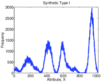
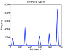
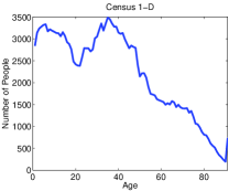
We conduct experiments for one-dimensional case using two different types of synthetic data and a $1$-D projection of Census data (see Figure 1 (a),(b),(c) for the data distributions of the above three datasets):

• Synthetic Type I: For this dataset, we sampled points from a mixture of seventeen Gaussians, each with variance $625$ and means selected uniformly at random from $[0,r]$.

• Synthetic Type II: Here, we sampled from a mixture of five Gaussians and means of each Gaussian is selected uniformly at random. The variance is selected to be just $100$, leading to “spiky” distribution, i.e., most records are concentrated around a small number of attribute-values.

• Census 1-D: We use the Age attribute of the standard Census dataset with $199,523$ database records. Range ($r$) here is $91$.

Similarly, for multi-dimensional histogram experiments, we generated synthetic data using multi-dimensional Gaussians and use multi-dimensional projections of Census data. That is,

• Synthetic Multi-D: We generated 2 and 3 dimensional datasets for a given range by sampling from a mixture of spherical Gaussians of corresponding number of dimensions. For 2-dimensional datasets, we used a mixture of 9 Gaussians with random means and variance equal to 100. For 3-dimensional case we used a mixture of 5 Gaussians with random means and variance set to 25. The range along each attribute was fixed to 32.

• Census Multi-D: We used the $2$-dimensional dataset obtained by selecting the “Age” and “Number of Weeks worked” attributes. For the $3$-dimensional dataset we chose the attributes of “Age”, “Marital status” and “Education”.

Given the above datasets, we now describe the models to generate QFRs used for training and testing learned histograms. We used two standard models of range query generation models proposed by [17] and later used by [2]:

• Data-dependent Query Model: In this model, first query “center” is sampled from the underlying data distribution. Then, the query is given by a hyper-rectangle whose centroid is given by the generated “center” and whose volume is at most $20$% of the total volume.

• Uniform Query Model: In this model, query “centers” are selected uniformly at random from the data range. Then, similar to the above query model, each query is a hyper-rectangle generated around the “center” and volume at most $20$% of the total volume.

As mentioned in [2], the above two models are considered to be fairly realistic and mimics many real-world query workloads. We generated separate training and test sets (of QFRs) in all the experiments. In each of the experiments, we evaluated various methods using a test set of $5000$ QFRs.

Implementation Details: For experiments with one-dimensional histograms, we implemented both of our methods EquiHist and SpHist, as well as ISOMER using Matlab. We modified an C++ implementation of STHoles [2] for multi-dimensional histograms experiments. For these experiments, we implemented both ISOMER as well as our equi-width approach (EquiHist) using C++. SpHist was implemented in MATLAB. For each experiment, we report numbers averaged over 10 runs.

For solving the max-entropy problem in ISOMER, we use an iterative solver based on Bregman’s method [6]. We found Bregman’s method for solving max-entropy problem to be significant faster than the Iterative Scaling method used by [21].

4.2 Results for One-Dimensional Histograms

(a)	(b)	(c)	(d)

Figure 2: Comparison of average relative error (on log-scale) with varying number of training queries. (a) Test error for Synthetic Type I dataset with queries generated from Uniform Query model. Both EquiHist and SpHist converges at around $200$ training queries only, and incurs $0.5\%$ and $1.4\%$ less error than ISOMER, respectively, for $700$ training queries. (b) Test error on Synthetic Type I dataset with queries generated from Data-dependent Query Model. Here again, both EquiHist and SpHist converges at around $200$ training queries and are finally obtains $0.3\%$ and $1.6\%$ less error than ISOMER. (c) Test error on “spiky” Synthetic Type II dataset with queries from Data-dependent Query model. For $700$ training queries, ISOMER incurs $26.87\%$ error, while SpHist incurs only $1.37\%$ error. (d) Test error on the Age attribute of Census $1$-d data with queries generate from Uniform Query model. For $200$ queries, EquiHist incurs approximately $0.5\%$ less error than ISOMER, while SpHist incurs $1.5\%$ less error.

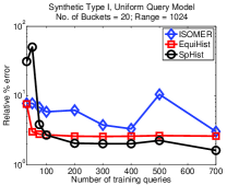
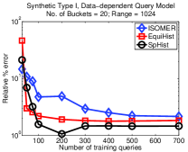
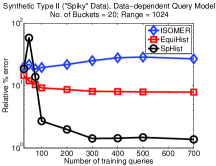
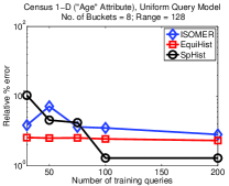
We now present results for 1-D histograms and study how the performance varies under different conditions: first, as the number of training queries increases, second, as the number of buckets in the histogram being learnt increases, and finally, as the range of attribute value increases.
Varying Number of Training Queries:
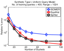
We first compare our EquiHist and SpHist method with ISOMER for varying number of training queries. Figure 2 (a) compares relative error incurred on test queries by the three methods on Synthetic Type I dataset for queries generated from Uniform Query Model. Here, we vary the number of training queries from $25$ to $700$, while the range $r$ of attribute values is fixed to be $1024$ and the number of buckets in the histogram is fixed to be $20$. Naturally, the error incurred by each of the methods decreases with increasing number of training queries. However, both of our methods are able to decrease the relative error more rapidly. For example, in around $200$ queries, error converges for both EquiHist and SpHist. In contrast, error incurred by ISOMER decreases slowly and oscillates, primary reason being in the final round ISOMER uses only twice the number of queries (approximately) as number of buckets ($20$) and hence over-fits in some runs. Furthermore, even with $700$ queries, our SpHist method is $1.4\%$ more accurate than ISOMER, while EquiHist is $0.5\%$ more accurate.

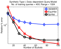
Next, we compare the three methods on Synthetic Type I dataset with queries generated from Data-dependent Query Model (See Fig. 2 (b)). Here again, both EquiHist and SpHist requires only $300$ training queries to converge, and are about $0.3\%$ and $1.6\%$ more accurate than ISOMER.

Figure 3: Figure shows learned histogram by ISOMER (top plot), EquiHist (middle plot) and SpHist (bottom plot) for “spiky” Synthetic Type II dataset with $700$ data-dependent queries and $20$ buckets. Clearly, bucket boundaries discovered by ISOMER do not align well with the peaks of the true frequency distribution(see Figure 2 (c)), leading to high error. EquiHist is constrained to partition range at equal intervals, hence is mis-aligned with several peaks. In contrast, SpHist is able to accurately align bucket boundaries to the true frequency distribution, hence incurs less test error.

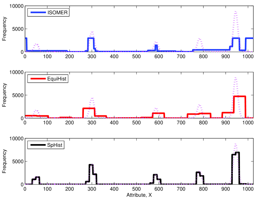
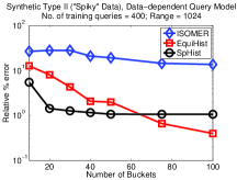
In Fig. 2 (c) we compare performances on the spiky Synthetic Type II dataset with queries generated from Data-dependent Query Model. For this experiment, all the three methods converge at about $300$ queries. However, SpHist is significantly more accurate than both ISOMER and EquiHist. Specifically, SpHist incurs only $1.37\%$ error, while EquiHist incurs $7.85\%$ error and ISOMER incurs $26.87\%$ error. EquiHist naturally is a little inaccurate as EquiHist’s bin boundaries will typically be much wider than optimal histograms boundaries. Interestingly, SpHist is able to learn correct bucket boundaries with small number of training queries and hence provides a histogram very similar to the underlying distribution. Figure 3 shows the recovered histograms by the different methods overlayed on the true frequency distribution. We observe that SpHist is able to align bin boundaries accurately with respect to the true distribution. In comparison, ISOMER and EquiHist’s buckets are not as well aligned, leading to higher test errors.

In Fig. 2 (d) we compare the three methods on the Census 1-D dataset and queries generated from Uniform Query Model. As in the previous case, SpHist incurs less error than both ISOMER and EquiHist ($1.5\%$ and $1.0\%$ less error respectively), and is able to learn from a smaller number of training queries.

(a)	(b)	(c)	(d)

Figure 4: Comparison of average relative error (on log-scale) with varying number of histogram buckets. (a) Test error on Synthetic Type I datasets with queries generated from Uniform Query model. For most values, both EquiHist and SpHist are significantly more accurate than ISOMER. As expected, for small number of buckets, SpHist is more accurate than EquiHist while for large number of buckets, EquiHist incurs less error. In particular, for $10$ buckets, SpHist is $18\%$ more accurate than ISOMER and $6\%$ more accurate than EquiHist. (b) Test error on Synthetic Type I dataset with queries generated from Data-dependent Query Model. Here again, SpHist is around $5\%$ more accurate than EquiHist for $10$ buckets and is around $0.3\%$ less accurate than ISOMER. (c) Test error on Synthetic Type II dataset with queries from Data-dependent Query model. Here, SpHist incurs significantly less error than both ISOMER (by $21\%$) and EquiHist (by $6\%$) for $10$ buckets. (d) Test error on Census 1-D dataset with queries generate from Uniform Query model. For $5$ buckets, SpHist incurs about $2\%$ less error than EquiHist and $20\%$ less error than ISOMER.

Varying Number of Buckets:
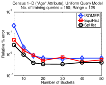
Here, we study our methods as number of buckets in the histograms vary. First, we consider Synthetic Type I dataset and vary number of buckets from $10$ to $100$, while range and number of training queries are fixed to be $1024$ and $400$, respectively. Figure 4 (a) shows error incurred by the three methods for varying number of buckets when queries are generated using Uniform Query Model. Clearly, for small number of buckets, SpHist achieves significantly better error rates than EquiHist and ISOMER. Specifically, for $10$ buckets, SpHist incurs $8.3\%$ error, while EquiHist incurs $14.09\%$ error and ISOMER incurs $26.84\%$ error. However, EquiHist performs better than both ISOMER and SpHist as number of buckets increase. Figure 4 (b) shows a similar trend when queries are generated from Data-dependent Query Model. Here, interestingly, for $10$ buckets, ISOMER performs significantly better than EquiHist and performs similar to SpHist. However, with larger number of buckets ISOMER converges to significantly higher error than both EquiHist and SpHist.

Next, we consider the Synthetic Type II dataset with Data-dependent Query Model and vary number of buckets from $10$ to $1000$. Figure 4 (c) compares test error incurred by the three methods. Here again, SpHist performs best of the three methods. In particular, for $10$ buckets, SpHist incurs $5.48\%$ error while EquiHist incurs $12.68\%$ error and ISOMER incurs $26.66\%$ error.

Finally, we consider Census 1-D data with queries drawn from Uniform Query Model. We vary the number of buckets from $5$ to $50$; note that the range of Age attribute is only $91$. Similar to the above experiments, SpHist incurs significantly less error than ISOMER (by $20\%$) and EquiHist (by $2\%$).

Varying Range of Attribute Values:
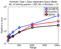
In the next experiment, we study performance of the different methods for varying range of attribute values. Here, we use Synthetic Type I dataset with Data-dependent Query Model and fix the number of buckets to $15$, the number of training queries are fixed to be $200$. Figure 1 (d) compares error incurred by SpHist and EquiHist to ISOMER on Synthetic Type I dataset with queries from Data-dependent Query Model. Here again, our methods are significantly better than ISOMER. Also, as predicted by our theoretical results (see Theorem 2), EquiHist does not depend heavily on the range and is able to learn low-error histograms with small number of queries. Similar trends were observed for Uniform Query Model and Synthetic Type II data as well.

We summarize our results for $1$-dimensional histogram settings as follows:

•  Both EquiHist and SpHist converge quicker than ISOMER with respect to number of queries and in general incurs less error for all training queries numbers.

•  SpHist incurs significantly less error than EquiHist and ISOMER for “spiky” data (Synthetic Type II dataset).

•  EquiHist and SpHist consistently outperform ISOMER with varying number of buckets.

•  SpHist demonstrates a clear advantage over the other two methods for smaller number of buckets. For larger number of buckets, EquiHist incurs less error than SpHist.
•  Both EquiHist and SpHist scale well with increasing range of the attribute values.

4.3 Multi-dimensional Histograms

In this section, we empirically compare our EquiHist and SpHist methods with ISOMER for learning multi-dimensional histograms. For these experiments also, we use synthetic as well Census data. Also, we use Data-dependent Query Model for all the multi-dimensional histogram experiments.

(a)	(b)	(c)	(d)

Figure 5: Comparison of average relative error (on log-scale) for various methods on two-dimensional datasets with queries generated from Data-dependent Query model. (a) Test error on Synthetic 2-D dataset with varying number of training queries. For $1200$ queries, both SpHist and EquiHist incurs about $26\%$ less error than ISOMER. (b) Test error for Synthetic 2-D dataset with varying number of buckets. For $16$ buckets, SpHist incurs $13.95\%$ error while EquiHist incurs $26.68\%$ error and ISOMER incurs $33.99\%$ error. (c) Test error for Census 2-D data with varying number of training queries. For $1200$ queries, SpHist incurs $4.64\%$ error, while EquiHist incurs $109.54\%$ error and ISOMER incurs $35.55\%$ error. EquiHist incurs more error than both SpHist and ISOMER due to “spikiness” of the data (see Figure 7 (a)). (d) Test error for Census 2-D data with varying number of histogram buckets. For $16$ buckets, SpHist incurs $10.21\%$ error while ISOMER incurs $66.34\%$ error and EquiHist incurs $148.7\%$ error. Similar to plot (b), EquiHist incurs larger error due to heavily skewed data (see Figure 7 (a)).

(a)	(b)	(c)	(d)

Figure 6: Comparison of average relative error (on log-scale) for various methods on three-dimensional datasets with queries generated from Data-dependent Query model. a), b) Test error on Synthetic 3-D dataset with varying number of training queries and varying number of buckets. Here, both EquiHist and SpHist are able to learn reasonable histograms (incurs about $10\%$ error) and follow similar trends to two-dimensional experiments (see Figure 5). We do not report test error for ISOMER, as our implementation of ISOMER did not finish even after two days, c), d) Test error on Census 3-D dataset with varying number of training queries and number of buckets . Similar to Census 2-D dataset, SpHist incurs significantly less error than both EquiHist and ISOMER. For example, in plot (c), for $1500$ queries, SpHist incurs about $11\%$ less error than ISOMER and $30\%$ less error than EquiHist.

(a)	(b)	(c)	(d)

Figure 7: a) Frequency distribution of “Age” and “Number of Weeks Worked” attributes of Census $2$-D data, b) Estimated histogram for Census $2$-D data using SpHist method with $1000$ training queries and $64$ buckets (See plot (a) for true distribution). SpHist is able to recover the underlying distribution well using small number of buckets and training queries. In particular, the high density areas for “Weeks Worked” attribute values $0$ and $52$ are captured accurately, c) Running times of SpHist and EquiHist for Synthetic $3$-D dataset (on a dual-core 2GHz processor with 4GB RAM). Note that our methods mostly finish with in 30 seconds, while on the same experiment our implementation of ISOMER did not finish in 2 days, d) Streaming queries and database updates experiment. Test error incurred by online version of EquiHist as well as batch version for Synthetic Type I dataset. At each step, one training query is provided; at $1000$-th step database is updated by randomly permuting $30\%$ of the database. EquiHist (1-1000) represents batch Equihist histogram obtained by training on first $1000$ queries, while EquiHist(1001-2000) trains on the batch of $1001-2000$-th queries.

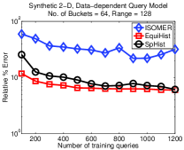
Experiments with 2-dimensional Datasets: We first compare our methods to ISOMER for varying number of training queries on Synthetic 2-D dataset. Figure 5 (a) shows the test error obtained by all the three methods for different number of training queries, where queries are generated using Data-dependent Query Model and the number of histogram buckets is fixed to be $64$. Clearly, our methods outperform ISOMER and are able to reduce error rapidly with increasing number of training queries. For example, for $1000$ training queries, both SpHist and EquiHist incurs about $6.0\%$ error while ISOMER incurs $31\%$ error.

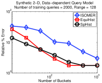
Next, we compare the three methods on Synthetic 2-D dataset, while varying number of buckets, with number of training queries is fixed at $2000$ (see Figure 5 (b)). Here again, both EquiHist and SpHist outperform ISOMER for small number of buckets. For $128$ buckets, ISOMER incurs $10.36\%$ error while EquiHist and SphHist incur around $2.91\%$ and $3.83\%$ error respectively.

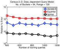
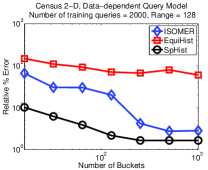
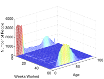
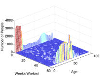
In the next set of experiments, we compare the performance of the three algorithms on real-world Census 2-D dataset (see Figure 5 (c)). Recall that Census 2-D dataset projects Census data on “Age” and “Number of Weeks Worked” attributes. Now, for most database records, “Number of Weeks Worked” are concentrated around either $0$ or $53$ weeks. That is, the data is extremely “spiky”. However, EquiHist still tries to approximate the entire space using equi-width buckets leading to several “empty” buckets. Consequently, EquiHist incurs large error ($109\%$ for $1200$ queries), while ISOMER also incurs $35.55\%$ error. However, SpHist is still able to approximate the underlying distribution well and incurs only $4.64\%$ error. Figure 7 (b) shows the histogram estimated by SpHist with $1000$ queries and $64$ buckets. Clearly, SpHist is able to capture high-density regions well; there are small peaks in low-density areas which contribute to the error that SpHist incurs.

Finally, we report test error incurred by the three methods on Census-2D dataset in Figure 5 (d), as we vary the number of buckets from $5$ to $2048$, while number of training queries is fixed at $2000$. For this data as well, SpHist outperforms both EquiHist and ISOMER significantly, especially for small number of buckets. Specifically, for $16$ buckets, SpHist incurs only $10.21\%$ relative error while EquiHist and ISOMER incur about $148.7\%$ and $66.34\%$ relative error, respectively.
3-dimensional Datasets: We now consider $3$-dimensional datasets to study scalability of our methods with increasing dimensions.

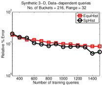
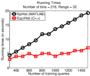
We first conduct experiments on the Synthetic 3-D dataset, which is drawn from a mixture of spherical 3-D Gaussians. Figure 6 (a) shows relative error incurred by our methods when queries are generated from Data-dependent Query Model and the number of training queries vary, while number of buckets is fixed at $216$. For $2000$ queries, SpHist incurs $5.59\%$ error while EquiHist incurs $8.39\%$ error. Note that we are not able to report error incurred by ISOMER as our implementation of ISOMER did not terminate even after running for two days. Primary reason being, even in 3-dimensions, number of variables in ISOMER’s max-entropy problem becomes large, e.g., for our experiments with $1000$ queries ISOMER had $27,000$ variables in the first round. Furthermore, ISOMER needs to iteratively re-optimize after throwing out a fixed number of queries, thus further increasing run-times. In contrast, both of our methods are very efficient, and need to run the optimization only once. We observed that in all our experiments, our methods terminated in less than $1$ minutes (see Figure 7(c)).

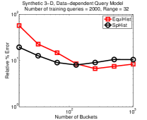
Next, we vary number of buckets while number of training queries is fixed to be $2000$. Figure 6 (b) shows relative error incurred by our methods. Clearly, for small number of buckets SpHist is significantly better than EquiHist. For example, for $16$ buckets SpHist incurs $19.51\%$ error while EquiHist incurs $57.36\%$ error.

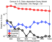
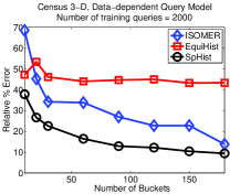
Finally, we repeat these experiments on our Census 3-D dataset (which, considers the “Age”, “Marital Status” and “Education” as the 3 attributes), i.e., we vary number of training queries (Figure 6 (c)) as well as number of buckets (Figure 6(d)). Overall, we observe the same trend as 2-dimensional case with SpHist being most accurate and EquiHist being most inaccurate, e.g., for $200$ buckets SpHist incurs $7\%$ error while ISOMER incurs $20\%$ error and EquiHist incurs $38\%$ error.

4.4 Dynamic QFRs and data updates

We now study the performance of online version of EquiHist (Section 3.5) for dynamic QFRs and in the presence of data updates. (The performance of online SpHist is similar when the set ${\mathcal{S}}$ of non-zero wavelet coefficients is kept unchanged.) The goal is to show that our online updates are effective, converge to the optimal batch solution quickly, and are robust to database updates.

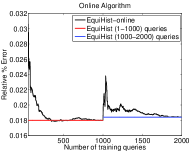
For this experiment, we consider Synthetic Type I dataset with queries generated from the Uniform Query Model. We compare our online version of EquiHist against the batch-version of EquiHist. After each update of the online version, we measure relative error on $5000$ test queries. We also, measure relative test error incurred by the batch EquiHist method (that can observe all the training queries beforehand). Figure 7 (d) compares relative error incurred by online EquiHist to batch method. For $1$ to $1000$ steps, the database remains the same. Clearly, online learning algorithm quickly (in around $250$ steps) converges to relative error similar to batch method (red line) with $1000$ training queries.

Now at $1000$-th step, we update our database by randomly perturbing $30\%$ of the database. This leads to larger error for online EquiHist for a few steps after $1000$-th step (see Figure 7 (d)), however it quickly converges to the optimal batch solution (blue line) for the updated database (using queries $1001$ to $2000$).

4.5 Comparison to ISOMER

Here, we summarize our experimental results and discuss some of the advantages that our method enjoys over ISOMER.

•  ISOMER reduces the number of histogram buckets by removing queries. Hence for small number of buckets, ISOMER removes almost all the queries and ends up over-fitting to a few queries, leading to high relative error. In contrast, our methods use all the queries and hence are able to generalize significantly better.

•  ISOMER has to re-run max-entropy solver after each query-reduction step, hence time required by ISOMER is significantly larger than our methods.

•  For multi-dimensional case, ISOMER’s data structure forms large number of buckets even though the final number of buckets required is small. For this reason, ISOMER doesn’t scale well to high-dimensions; in contrast, our method apriori fixes the number of buckets and hence scales fairly well with high-dimensions.

•  Database updates lead to inconsistent QFRs, which which needs to be thrown away by ISOMER in a heuristic manner. In comparison, our methods easily extend to database updates.

5 Related Work

Simplicity and efficiency of histograms have made them the choice data-structure to summarize information for cardinality estimation, a critical component of query optimization. Consequently, histograms are used in most commercial database systems. Most of the prior work on histograms has focused on constructing and maintaining histograms from data, and we refer the reader to [11] for a survey.

Self-tuning histograms were first introduced by [1] to exploit workload information for more accurate cardinality estimation. The method proposed in [1] is typically referred to as STGrid and it merges and splits buckets according to bin densities. However, it does not have any known provable bounds on the expected relative error and is restricted by the grid structure for high-dimensional cases. [3] introduced STHoles data-structure which is significantly more powerful than the simple grid structure used by STGrid. However, this method requires fine-grained query feedback corresponding to each bucket in the current histogram and therefore imposes a nontrivial overhead while collecting feedback. Furthermore, if the number of queries is small then STHoles is not “consistent”, i.e., different ways of constructing data-structure can lead to different query cardinality estimations . This consistency problem was addressed by [21] who designed a maximum entropy based method called ISOMER. ISOMER uses a data-structure similar to STHoles, but learns frequency values in each bucket using a maximum-entropy solution. Note that, ISOMER is considered to be the state-of-the-art method for self-tuning histograms [8] and hence we compare against the same both theoretically as well as empirically. Recent work [13, 19] has extended to maximum entropy approach to handle feedback involving distinct values. [13] also present a histogram construction that is similar to EquiHist, but this algorithm only handles 1-dimensional histograms. Self-tuning histograms are part of a larger effort that seeks to leverage execution feedback for query optimization [15].

Wavelets are a popular signal-processing tool for compressing signals. Haar wavelets are one of the most popular and simple wavelets that are especially effective for piecewise constant signals. As histograms are piecewise constant signals, Haar wavelets are extensively used in the context of databases. Specifically, [16] introduced a wavelet based histogram that can be used for selectivity estimation. Similarly, [7] also defined a method for selectivity estimation using wavelets. [10] introduced a probabilistic method to decide the wavelet coefficients to be used and provides error guarantees for the same. However, most of these methods compute wavelets coefficients using a complete scan of the database and are not self-tuning. In contrast, we introduce a method that uses sparse-vector recovery techniques to learn appropriate wavelet coefficients for estimating self-tuning histograms.

6 Conclusions

In this paper, we introduced a learning theoretic framework for the problem of self-tuning histograms. We cast the problem in an empirical loss minimization framework, and propose two different approaches in this framework. Our first approach (EquiHist) efficiently learns well-known equi-width histograms. We also show that the equi-width approach, despite limitations, can still solve our histogram estimation problem up to an additive approximation factor while requiring only a finite number of training queries. To the best of our knowledge, this is the first theoretical guarantee for equi-width histograms in the context of self-tuning histograms.

However, in high-dimensions where data is sparse or for “spiky” datasets, equi-width approach suffers as it wastes many buckets on empty region. Our second approach (SpHist) handles this problem where, by using Haar wavelet transform, we cast the problem as that of learning a sparse vector. Next, we adapt the popular Orthogonal Matching Pursuit (OMP) method [22] for solving the transformed problem.

Both of our techniques can be easily extended to multi-dimensional settings, dynamic QFRs and database updates. To demonstrate effectiveness of our methods in all these scenarios, we provide a variety of empirical results. Overall, our empirical results show that SpHist is consistently better than EquiHist as well as ISOMER, especially for multi-dimensional datasets as well as for small number of buckets—both critical parameters for real-world databases. For example, SpHist is able to recover back the true distribution reasonably well for Census 2-D dataset (see Figure 7(b)).

For future work, we intend to work on theoretical analysis of SpHist. Another interesting direction is further study of the multi-dimensional buckets output by SpHist, so as to further improve its efficiency. Finally, we intend to apply our techniques to real-world query workloads.

Appendix A Proofs of Equi-width Approach

A.1 Proof of Theorem 2

Proof A.5.

Now,

$$F(\hat{\mathbf{\bm{h}}})-F(\mathbf{\bm{h}}^{*}) =F(\hat{\mathbf{\bm{h}}})-F(\tilde{\mathbf{\bm{h}}})+F(\tilde{\mathbf{\bm{h}}})-F(\mathbf{\bm{h}}^{*}),$$ (30)

$$=E_{1}+E_{2},$$ (31)

where $\tilde{\mathbf{\bm{h}}}\in\mathcal{C}^{\prime}$ is given by $\tilde{\mathbf{\bm{h}}}=B\tilde{\mathbf{\bm{w}}}$, $\tilde{\mathbf{\bm{w}}}$ being the optimal solution to (15), $E_{1}=F(\hat{\mathbf{\bm{h}}})-F(\tilde{\mathbf{\bm{h}}})$ is the excess generalization error incurred by $\hat{\mathbf{\bm{h}}}$ compared to the optimal solution $\tilde{\mathbf{\bm{h}}}$ and $E_{2}=F(\tilde{\mathbf{\bm{h}}})-F(\mathbf{\bm{h}}^{*})$ is the difference between optimal error achievable by histograms in $\mathcal{C}^{\prime}$ to the histograms in $\mathcal{C}$. Intuitively, $E_{2}$ measures how expressive set $\mathcal{C}^{\prime}$ is w.r.t. $\mathcal{C}$. Below we bound both the error individually and finally combine the two errors to obtain error bound on $F(\hat{\mathbf{\bm{h}}})-F(\mathbf{\bm{h}}^{*})$.
Bound on $E_{1}$: Let $\tilde{\mathbf{\bm{h}}}=B\tilde{\mathbf{\bm{w}}}$. Now, since $G_{\mathcal{D}}(\cdot)$ is the regularized expected risk under a convex risk function ($f(\mathbf{\bm{q}}^{T}B\mathbf{\bm{w}};s_{q})$) we can use standard results from stochastic convex optimization to bound the generalization error. In particular, using Theorem 3 by [20], with probability $1-\delta$:

$$\mathbb{E}_{\mathbf{\bm{q}}\sim\mathcal{D}}[f(\mathbf{\bm{q}}^{T}B\hat{\mathbf{\bm{w}}};s_{\mathbf{\bm{q}}})]-\lambda H(\frac{r}{Mb}\hat{\mathbf{\bm{w}}})\leq\mathbb{E}_{\mathbf{\bm{q}}\sim\mathcal{D}}[f(\mathbf{\bm{q}}^{T}B\tilde{\mathbf{\bm{w}}};s_{\mathbf{\bm{q}}})]\\ -\lambda H(\frac{r}{Mb}\tilde{\mathbf{\bm{w}}})+O\left(\frac{\Omega^{2}L_{f}^{2}M^{2}b\log\frac{1}{\delta}}{r\Delta\lambda N}\right),$$ (32)

where:

• $\Omega=\max_{\mathbf{\bm{q}}\sim\mathcal{D}}\|B^{T}\mathbf{\bm{q}}\|$. Assuming each query covers only $|Q|$ attribute values, $\Omega=|Q|$.

• $L_{f}$ is the Lipschitz constant of function $f(u;s_{q})$ w.r.t. $u$. Note that as $\mathcal{K}$ is a compact set, $L_{f}\leq\max_{u\in\Omega\|\mathcal{K}\|_{2}}\|{\nabla}f(u)\|_{2}$.

• $\lambda>0$ is a constant. Also, note that entropy function $H(\frac{r}{Mb}\mathbf{\bm{w}})$ is $\frac{r\Delta}{M^{2}b}$-strongly convex.

Now, $H(\frac{r}{Mb}\hat{\mathbf{\bm{w}}})\leq\log b$. Hence, using (32),

$$F(\hat{\mathbf{\bm{w}}})-F(\tilde{\mathbf{\bm{w}}}) \leq\lambda\log b+O\left(\frac{|Q|^{2}L_{f}^{2}M^{2}b\log\frac{1}{\delta}}{r\Delta\lambda N}\right),$$

$$\leq O\left(\sqrt{\frac{b\log b\log\frac{1}{\delta}}{r\Delta N}}M|Q|L_{f}\right),$$ (33)

where the second inequality follows by selecting

$$\lambda=\sqrt{\frac{b\log\frac{1}{\delta}}{r\log b\Delta N}}M|Q|L_{f}.$$

That is,

$$E_{1}=F(\hat{\mathbf{\bm{h}}})-F(\tilde{\mathbf{\bm{h}}})=F(\hat{\mathbf{\bm{w}}})-F(\tilde{\mathbf{\bm{w}}})\\ \leq O(\sqrt{\frac{b\log b\log\frac{1}{\delta}}{r\Delta N}}M|Q|L_{f}).$$ (34)

Bound on $E_{2}$: To bound $E_{2}$, we first observe that

$$F(\tilde{\mathbf{\bm{h}}})\leq F(\mathbf{\bm{h}})+\lambda\log b,\forall\mathbf{\bm{h}}\in\mathcal{C}^{\prime}.$$

Hence,

$$E_{2}\leq F(\mathbf{\bm{h}})-F(\mathbf{\bm{h}}^{*})+E_{1},\forall\mathbf{\bm{h}}\in\mathcal{C}^{\prime}.$$ (35)

Now, given any $\mathbf{\bm{h}}^{*}$ we construct a new vector $\overline{\mathbf{\bm{h}}}^{*}\in\mathcal{C}^{\prime}$ for which we can bound the error $F(\overline{\mathbf{\bm{h}}}^{*})-F(\mathbf{\bm{h}}^{*})$.

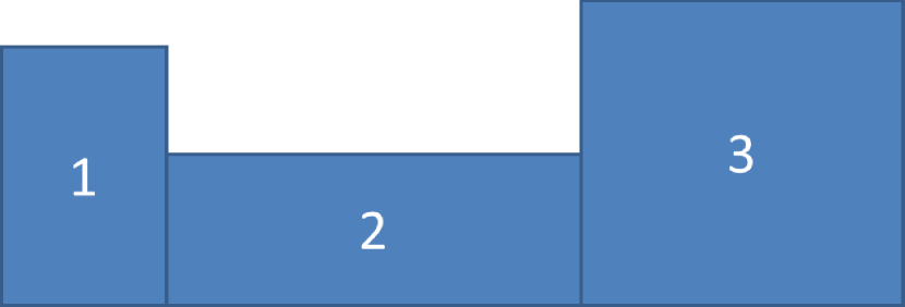
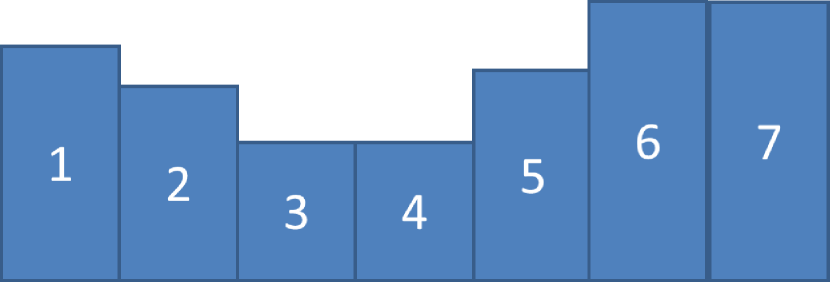
Now, $\overline{\mathbf{\bm{h}}}^{*}$ has $b$ buckets and each the value in each bucket ( i.e., $\overline{\mathbf{\bm{w}}}^{*}_{i},1\leq b$) is the average of the histogram heights of $\mathbf{\bm{h}}^{*}$ in that particular bucket. Formally,

$$\overline{\mathbf{\bm{w}}}^{*}_{i}=\frac{1}{r/b}\sum_{j=\frac{r}{b}(i-1)}^{\frac{r}{b}\cdot i}\mathbf{\bm{h}}^{*}_{j}.$$ (36)

See Figure 8 for an illustration of our conversion scheme from $\mathbf{\bm{h}}^{*}$ to $\overline{\mathbf{\bm{h}}}^{*}$.

Figure 8: Conversion of $\mathbf{\bm{h}}^{*}$ to $\overline{\mathbf{\bm{h}}}^{*}$. Top figure shows $\mathbf{\bm{h}}^{*}$ while the bottom one shows $\overline{\mathbf{\bm{h}}}^{*}$. Note that buckets 1,3,4,6,7 of $\overline{\mathbf{\bm{h}}}^{*}$ lie with-in buckets of $\mathbf{\bm{h}}^{*}$, hence we assign same heights to them as the corresponding buckets in $\mathbf{\bm{h}}^{*}$. Buckets 2, 5 of $\overline{\mathbf{\bm{h}}}^{*}$ are at the intersection of of buckets 1 and 2, 2 and 3 of $\mathbf{\bm{h}}^{*}$, hence a convex combination of heights of those buckets are assigned to Buckets 2, 5 of $\overline{\mathbf{\bm{h}}}^{*}$.

Now, note that,

$$\sum_{j=1}^{r}\overline{\mathbf{\bm{h}}}^{*}_{j}=\sum_{j=1}^{r}\mathbf{\bm{h}}^{*}=M.$$

Furthermore, assuming $\frac{r}{b}\leq\Delta$ (i.e., width of buckets in $\overline{\mathbf{\bm{h}}}^{*}$ is smaller than the smallest bucket of $\mathbf{\bm{h}}^{*}$), average is over at most two different heights of $\mathbf{\bm{h}}^{*}$ in each bucket of $\overline{\mathbf{\bm{h}}}^{*}$. Since there are only $k$ buckets in $\mathbf{\bm{h}}^{*}$, only $k-1$ buckets in $\overline{\mathbf{\bm{h}}}^{*}$ are at the intersection of buckets in $\mathbf{\bm{h}}^{*}$. Let $I$ be the set of all the buckets in $\overline{\mathbf{\bm{h}}}^{*}$ that are at intersection of buckets in $\mathbf{\bm{h}}^{*}$. Now consider $\|\mathbf{\bm{h}}^{*}-\overline{\mathbf{\bm{h}}}^{*}\|_{2}^{2}$. Clearly, if a bucket in $\overline{\mathbf{\bm{h}}}^{*}$ do not lie in $\mathbf{\bm{h}}^{*}$ then it do not contribute to $\|\mathbf{\bm{h}}^{*}-\overline{\mathbf{\bm{h}}}^{*}\|_{2}^{2}$, as value of attributes in that bucket is same as the value of attributes in the corresponding bucket of $\mathbf{\bm{h}}^{*}$. Thus,

$$\|\mathbf{\bm{h}}^{*}-\overline{\mathbf{\bm{h}}}^{*}\|_{2}^{2}=\sum_{J\in I}\sum_{i\in J}(\mathbf{\bm{h}}^{*}_{i}-\overline{\mathbf{\bm{h}}}^{*}_{i})^{2}\leq\sum_{J\in I}\sum_{i\in J}(\mathbf{\bm{h}}^{*}_{i})^{2}\leq\frac{r}{b}\sum_{J\in I}h_{i}^{*}\|\mathbf{\bm{h}}^{*}\|_{\infty},.$$ (37)

where last inequality follows using Cauchy-Schwarz inequality. Now, $\|\mathbf{\bm{h}}^{*}\|_{\infty}\leq\frac{M}{\Delta}$, as each bucket is of at least $\Delta$ width and there are at most $M$ records to fill in one bucket. Similarly,

$$\Delta\sum_{J\in I}h_{i}^{*}\leq\|\mathbf{\bm{h}}^{*}\|_{1}=M.$$

Hence, using (37), with the above observations

$$\|\mathbf{\bm{h}}^{*}-\overline{\mathbf{\bm{h}}}^{*}\|_{2}\leq\frac{M}{\Delta}\sqrt{\frac{r}{b}}.$$ (38)

Now, we bound $F(\mathbf{\bm{h}}^{*})-F(\overline{\mathbf{\bm{h}}}^{*})$:

$$F(\mathbf{\bm{h}}^{*})-F(\overline{\mathbf{\bm{h}}}^{*}) =\mathbb{E}_{\mathbf{\bm{q}}\sim\mathcal{D}}[f(\mathbf{\bm{q}}^{T}\mathbf{\bm{h}}^{*};s_{q})-f(\mathbf{\bm{q}}^{T}\overline{\mathbf{\bm{h}}}^{*};s_{q})],$$

$$\leq\mathbb{E}_{\mathbf{\bm{q}}\sim\mathcal{D}}[L_{f}|\mathbf{\bm{q}}^{T}\overline{\mathbf{\bm{h}}}^{*}-\mathbf{\bm{q}}^{T}\mathbf{\bm{h}}^{*}|],$$

$$\leq\mathbb{E}_{\mathbf{\bm{q}}\sim\mathcal{D}}[L_{f}\|\mathbf{\bm{q}}\|_{2}\|\mathbf{\bm{h}}^{*}-\overline{\mathbf{\bm{h}}}^{*}\|_{2}],$$

$$\leq\sqrt{|Q|}L_{f}\frac{M}{\Delta}\sqrt{\frac{r}{b}},$$ (39)

where last inequality follows from the fact that $\mathbf{\bm{q}}$ is over $|Q|$ attributes only and using (38).

Now using (39) and (35):

$$E_{2}\leq\sqrt{|Q|}L_{f}\frac{M}{\Delta}\sqrt{\frac{r}{b}}+E_{1}.$$ (40)

Hence, by combining (31), (34), (40):

$$F(\hat{\mathbf{\bm{h}}})-F(\mathbf{\bm{h}}^{*}) \leq\sqrt{|Q|}L_{f}\frac{M}{\Delta}\sqrt{\frac{r}{b}}$$

$$\qquad+O\left(\sqrt{\frac{b\log b\log\frac{1}{\delta}}{r\Delta N}}M|Q|L_{f}\right),$$

$$\leq M\left(L_{f}\left(\frac{|Q|}{\Delta}\right)^{3/4}\left(\frac{\log\frac{1}{\delta}}{N}\right)^{1/4}\right),$$

$$\leq M\epsilon,$$ (41)

where last inequality follows by selecting N using:

$$N\geq C_{1}\left(\frac{|Q|}{\Delta}\right)^{3}\frac{L_{f}^{4}\log\frac{1}{\delta}}{\epsilon^{4}},$$ (42)

where $C_{1}>0$ is a constant. Now, second inequality in (41) follows by selecting $b$ using:

$$b=C_{2}r\left(\left(\frac{1}{|Q|\Delta}\right)^{1/2}\left(\frac{N}{\log\frac{1}{\delta}}\right)^{1/2}\right)\\ \geq C_{2}r\frac{|Q|L_{f}^{2}}{\Delta^{2}\epsilon^{2}}\geq C_{2}k\frac{|Q|L_{f}^{2}}{\Delta\epsilon^{2}},$$ (43)

where last inequality follows using $k\geq\frac{r}{\Delta}$ as $\Delta$ is the minimum bucket width and $C_{2}>0$ is a constant.

Hence proved.

A.2 Proof of Theorem 4

Proof A.6.

Similar to proof of Theorem 2:

$$F(\hat{H})-F(H^{*}) =F(\hat{H})-F(\tilde{H})+F(\tilde{H})-F(H^{*}),$$ (44)

$$=E_{1}+E_{2},$$ (45)

where $\tilde{H}\in\mathcal{C}^{\prime}$ is given by $\tilde{H}=B\tilde{W}B^{T}$.

Recall that,

$$G_{\mathcal{D}}(W)=E_{\mathcal{D}}\left[f(\langle Q,BWB^{T}\rangle;s_{Q})\right]-\lambda H(\frac{r\cdot r}{Mb}W),$$ (46)

and $\tilde{W}$ is the optimal solution to (46). Also, $E_{1}=F(\hat{H})-F(\tilde{H})$ is the excess generalization error incurred by $\hat{H}$ compared to the optimal solution $\tilde{H}$ and $E_{2}=F(\tilde{H})-F(H^{*})$ is the difference between optimal error achievable by histograms in $\mathcal{C}^{\prime}$ to the histograms in $\mathcal{C}$. Below we bound both the errors individually:
Bound on $E_{1}$: Recall that $\tilde{H}=B\tilde{W}B^{T}$. Also, note that
$\langle Q,BWB^{T}\rangle=\langle B^{T}QB,W\rangle$ is the inner product function over matrices. As $G_{\mathcal{D}}(\cdot)$ is the regularized empirical risk under a convex risk function $f$, using Theorem 3, with probability $1-\delta$:

$$\mathbb{E}_{Q\sim\mathcal{D}}[f(\langle Q,B\hat{W}B^{T}\rangle;s_{Q})]-\lambda H(\frac{r^{2}}{Mb}\hat{W})\\ \leq\mathbb{E}_{Q\sim\mathcal{D}}[f(\langle Q,B\tilde{W}B^{T}\rangle;s_{Q})]-\lambda H(\frac{r^{2}}{Mb}\tilde{W})\\ +O\left(\frac{\Omega^{2}L_{f}^{2}M^{2}b\log\frac{1}{\delta}}{r\Delta\lambda N}\right),$$ (47)

where:

• $L_{f}$ is the Lipschitz constant of function $f(u;s_{q})$ w.r.t. $u$, over a finite set. Hence, $L_{f}\leq\max_{|u|\leq\Omega\|\mathcal{K}\|_{2}}\|{\nabla}f(u)\|_{2}$

• $\Omega=\max_{\mathbf{\bm{q}}\sim\mathcal{D}}\|B^{T}QB\|_{F}$. Assuming each query covers only $|Q|$ attribute values, $\Omega=|Q|$.

• $\lambda$ is a constant. Also, note that entropy function $H(\frac{r^{2}}{Mb}W)$ is $\frac{r^{2}\Delta}{M^{2}b}$-strongly convex.

Now, $H(\frac{r^{2}}{Mb}\hat{W})\leq\log b$. Hence, using (47),

$$F(\hat{\mathbf{\bm{w}}})-F(\tilde{\mathbf{\bm{w}}}) \leq\lambda\log b+O\left(\frac{L_{f}^{2}|Q|^{2}M^{2}b\log\frac{1}{\delta}}{r^{2}\Delta\lambda N}\right),$$

$$\leq O(\sqrt{\frac{b\log b\log\frac{1}{\delta}}{r^{2}\Delta N}}L_{f}M|Q|),$$ (48)

where the second inequality follows by selecting

$$\lambda=\sqrt{\frac{b\log\frac{1}{\delta}}{r^{2}\log b\Delta N}}M|Q|L_{f}.$$

That is,

$$E_{1}=F(\hat{H})-F(\tilde{H})=F(\hat{W})-F(\tilde{W})\\ \leq O\left(\sqrt{\frac{b\log b\log\frac{1}{\delta}}{r^{2}\Delta N}}L_{f}M|Q|\right).$$ (49)

Bound on $E_{2}$: To bound $E_{2}$, we first observe that

$$F(\tilde{H})\leq F(H)+\lambda\log b,\forall\ H\in\mathcal{C}^{\prime}.$$

Hence,

$$E_{2}\leq F(H)-F(H^{*})+E_{1},\forall H\in\mathcal{C}^{\prime}.$$ (50)

Now, given any $H^{*}$ we construct a new vector $\overline{H}^{*}\in\mathcal{C}^{\prime}$ for which we can bound the error $F(\overline{H}^{*})-F(H^{*})$.

Note that along any of the axis, the number of 1-dimensional buckets are at most $k$. Hence, using error analysis from 1-dimensional case (see Equation 38),

$$\|H^{*}-\overline{H}^{*}\|_{F}\leq\frac{M}{\Delta}\frac{r}{\sqrt{b_{1}}}.$$ (51)

Now, we bound $F(\mathbf{\bm{h}}^{*})-F(\overline{\mathbf{\bm{h}}}^{*})$:

$$F(H^{*})-F(\overline{H}^{*}) =\mathbb{E}_{Q\sim\mathcal{D}}[f(\langle Q,H^{*}\rangle;s_{Q})-f(\langle Q,\overline{H}^{*}\rangle;s_{Q})],$$

$$\leq\mathbb{E}_{Q\sim\mathcal{D}}[L_{f}|\langle Q,\overline{H}^{*}\rangle-\langle Q,H^{*}\rangle|],$$

$$\leq\mathbb{E}_{Q\sim\mathcal{D}}[L_{f}\|Q\|_{F}\|H^{*}-\overline{H}^{*}\|_{F}],$$

$$\leq L_{f}\sqrt{|Q|}\frac{M}{\Delta}\frac{r}{\sqrt{b_{1}}},$$ (52)

where the second inequality follows using Lipschitz property of $f$, and last inequality follows from the fact that $\mathbf{\bm{q}}$ is over $|Q|$ attributes only and using (51).

Now using (52) and (50):

$$E_{2}\leq L_{f}\sqrt{|Q|}\frac{M}{\Delta}\frac{r}{\sqrt{b_{1}}}+E_{1}.$$ (53)

Hence, by combining (45), (49), (53):

$$F(\hat{H})-F(H^{*}) \leq L_{f}\sqrt{|Q|}\frac{M}{\Delta}\frac{r}{\sqrt{b_{1}}}$$

$$\qquad+O\left(\sqrt{\frac{b\log b\log\frac{1}{\delta}}{r\Delta N}}M|Q|L_{f}\right),$$

$$\leq M\left(L_{f}\left(\frac{|Q|}{\Delta}\right)^{3/4}\left(\frac{\log\frac{1}{\delta}}{N}\right)^{1/4}\right),$$

$$\leq M\epsilon,$$ (54)

where last inequality follows by selecting N using:

$$N\geq\left(\frac{|Q|}{\Delta}\right)^{3}\frac{L_{f}^{4}\log\frac{1}{\delta}}{\epsilon^{4}}.$$ (55)

Now, second inequality in (54) follows by selecting $b$ using:

$$b=r^{4}\left(\left(\frac{1}{|Q|\Delta}\right)\left(\frac{N}{\log\frac{1}{\delta}}\right)\right)\geq r^{4}\frac{|Q|^{2}}{\Delta^{4}\epsilon^{4}}\geq k^{2}\frac{|Q|^{2}L_{f}^{2}}{\epsilon^{4}},$$ (56)

where last inequality follows using $k\geq\frac{r^{2}}{\Delta^{2}}$ as $\Delta$ is the minimum bucket width. Hence proved.

References

- [1] A. Aboulnaga and S. Chaudhuri. Self-tuning histograms: Building histograms without looking at data. In SIGMOD Conference, pages 181–192, 1999.
- [2] N. Bruno and S. Chaudhuri. Exploiting statistics on query expressions for optimization. In SIGMOD Conference, pages 263–274, 2002.
- [3] N. Bruno, S. Chaudhuri, and L. Gravano. Stholes: A multidimensional workload-aware histogram. In SIGMOD Conference, pages 211–222, 2001.
- [4] E. Candes. The restricted isometry property and its implications for compressed sensing. Compte Rendus de l’Academie des Sciences, Paris, Serie I, 1:589–592, 2008.
- [5] E. J. Candès and T. Tao. Decoding by linear programming. CoRR, abs/math/0502327, 2005.
- [6] Y. A. Censor and S. A. Zenios. Parallel Optimization: Theory, Algorithms and Applications. Oxford University Press, 1997.
- [7] K. Chakrabarti, M. N. Garofalakis, R. Rastogi, and K. Shim. Approximate query processing using wavelets. VLDB J., 10(2-3):199–223, 2001.
- [8] S. Chaudhuri and V. R. Narasayya. Self-tuning database systems: A decade of progress. In VLDB, pages 3–14, 2007.
- [9] A. Frank and A. Asuncion. UCI machine learning repository, 2010.
- [10] M. N. Garofalakis and P. B. Gibbons. Wavelet synopses with error guarantees. In SIGMOD Conference, pages 476–487, 2002.
- [11] Y. E. Ioannidis. The history of histograms (abridged). In VLDB, pages 19–30, 2003.
- [12] H. V. Jagadish, N. Koudas, S. Muthukrishnan, V. Poosala, K. C. Sevcik, and T. Suel. Optimal histograms with quality guarantees. In VLDB, pages 275–286, 1998.
- [13] R. Kaushik and D. Suciu. Consistent histograms in the presence of distinct value counts. PVLDB, 2(1):850–861, 2009.
- [14] S. Mallat. A Wavelet Tour of Signal Processing. AP Professional, London, 1997.
- [15] V. Markl, G. M. Lohman, and V. Raman. Leo: An autonomic query optimizer for db2. IBM Systems Journal, 42(1):98–106, 2003.
- [16] Y. Matias, J. S. Vitter, and M. Wang. Wavelet-based histograms for selectivity estimation. In SIGMOD Conference, pages 448–459, 1998.
- [17] B.-U. Pagel, H.-W. Six, H. Toben, and P. Widmayer. Towards an analysis of range query performance in spatial data structures. In PODS, pages 214–221, 1993.
- [18] A. Rakhlin. Lecture notes on online learning, 2009. http://www-stat.wharton.upenn.edu / rakhlin/papers/online_learning.pdf.
- [19] C. Ré and D. Suciu. Understanding cardinality estimation using entropy maximization. In PODS, pages 53–64, 2010.
- [20] S. Shalev-Shwartz, O. Shamir, N. Srebro, and K. Sridharan. Stochastic convex optimization. In COLT, 2009.
- [21] U. Srivastava, P. J. Haas, V. Markl, M. Kutsch, and T. M. Tran. Isomer: Consistent histogram construction using query feedback. In ICDE, page 39, 2006.
- [22] J. A. Tropp and A. C. Gilbert. Signal recovery from random measurements via orthogonal matching pursuit. IEEE Transactions on Information Theory, 53(12):4655–4666, 2007.
- [23] R. Viswanathan, P. Jain, S. Laxman, and A. Arasu. A learning framework for self-tuning histograms. Arxiv, abs/1111.7295, 2011.
- [24] J. S. Vitter and M. Wang. Approximate computation of multidimensional aggregates of sparse data using wavelets. In Proceedings of the 1999 ACM SIGMOD international conference on Management of data, SIGMOD ’99, pages 193–204, New York, NY, USA, 1999. ACM.