General approach for studying first-order phase transitions at low temperatures

Abstract

By combining different ideas, a general and efficient protocol to deal with discontinuous phase transitions at low temperatures is proposed. For small $T$’s, it is possible to derive a generic analytic expression for appropriate order parameters, whose coefficients are obtained from simple simulations. Once in such regimes simulations by standard algorithms are not reliable, an enhanced tempering method, the parallel tempering – accurate for small and intermediate system sizes with rather low computational cost – is used. Finally, from finite size analysis, one can obtain the thermodynamic limit. The procedure is illustrated for four distinct models, demonstrating its power, e.g., to locate coexistence lines and the phases density at the coexistence.

First-order phase transitions (FOPT) are ubiquitous in nature books-first-order , associated to a countless number of processes lebowitz . Moreover, they take place in different temperature scales, e.g., from 2800 K in the Earth core-mantle oganov-matyska to few and near zero Kelvin range (for many systems, in a rather similar way kuwahara ), or even being responsible for unique effects, but across a very broad range of $T$’s silvera . In special, FOPT at low temperatures underpin important phenomena, like field-induced metal-insulator transitions, magnetoresistance, superfluidity, and Bose-Einstein condensation, among many others.

So, it is understandable and desirable the multitude of approaches (mainly numerically janke given the difficulty to obtain general exact results pfister ) developed to study FOPT. In certain instances, nevertheless, many of them can face procedural difficulties, not leading to precise results for the sough thermodynamical quantities, say, the exact location of coexistence lines.

As particularly powerful methods we can cite cluster algorithms bouabci , multicanonical berg and Wang-Landau wang . In cluster, non-local configuration exchanges often ensure the crossing of even high free-energy barriers. But a drawback is its specialization: each model requires a specific and efficient algorithm to implement the transitions, not available in many cases. On the other hand, Wang-Landau and multicanonical are general and have been applied successfully in a great diversity of problems. However, the former may demand very large computational time to calculate the density of states, specially considering that the number of states can increases very fast with the system size pla . The latter relies on histogram reweighting techniques to obtain the appropriate averages, a difficult task for large systems (see, e.g., okamoto ).

Given so, here we present a protocol to study FOPT at low temperatures by means of direct and simple numerical simulations. Extending previous results fiore-carneiro , it considers around any transition a general parametric analytical expression for relevant thermodynamic quantities (like order parameter, density, magnetization, compressibility, etc). The parameters are then obtained by simulating small systems, making the approach computationally fast. Finally, from proper extrapolations, the correct thermodynamic limit is obtained. Once standard algorithms usually fail for FOPT at low $T$’s, even for small systems, we consider tempering methods (already shown reliable for FOPT, see fiore-luz-1 ; fiore-luz-2 and Refs. therein). Thus, we use the parallel tempering, PT, very efficient for small and intermediate system sizes. As we exemplify with four different lattices models, the approach leads to a precise way to determine the coexistence regions.

We begin recalling a rigorous analysis for finite systems having $\mathcal{N}$ coexisting phases at $\xi^{*}$, with $\xi$ an appropriate phase transition parameter control (e.g., temperature or chemical potential). It has been shown rBoKo that at low $T$’s and around $\xi^{*}$, the partition function is very accurately given by $Z=\sum_{n=1}^{\mathcal{N}}\,\alpha_{n}\,\exp[-\beta Vf_{n}]$, with $\beta=(kT)^{-1}$. For the phase $n$, $f_{n}$ is the (metastable) free energy rBoKo per volume $V$ and $\alpha_{n}$ is the degeneracy, resulting from eventual symmetries of the problem.

Next observe that $W=-\partial_{\xi}\ln[Z]/(\beta\,V)$ ($\partial_{x}\equiv\partial/\partial x$) is frequently the start point to calculate distinct order parameters (density, magnetization, etc). Since close to $\xi^{*}$, $f_{n}\approx f^{*}+f_{n}^{\prime*}\,y$ comment for $f_{n}^{\prime*}=\partial_{\xi^{*}}f_{n}(\xi^{*})$ and $y\equiv\xi-\xi^{*}$, we find the following general form for $W$:

$$W=(b_{1}+\sum_{n=2}^{\mathcal{N}}b_{n}\,\exp[-a_{n}y])/(1+\sum_{n=2}^{\mathcal{N}}c_{n}\,\exp[-a_{n}y]).$$ (1)

The coefficients $a_{n}$, $b_{n}$ and $c_{n}$ depend on $\xi^{*}$, $f_{n}^{\prime*}$, $T$, and other system parameters. But only the $a_{n}$’s are (linear) functions of $V$. Then, at the coexistence ($y=0$) $W$ is independent on the volume and for all $V$ the curves $W\times\xi$ cross at $\xi=\xi^{*}$. In this way, Eq. (1) can be used not only to locate the transition point, but also to determine the coexistence order parameters at the thermodynamic limit. Moreover, if the $f$’s are ordered such that $f_{1}^{\prime*}=f_{2}^{\prime*}=\ldots=f_{m}^{\prime*}<f_{m+1}^{\prime*}<\ldots<f_{k}^{\prime*}=f_{k+1}^{\prime*}=\ldots=f_{\mathcal{N}}^{\prime*}$, for $V\rightarrow\infty$ and $y\rightarrow 0^{\pm}$ we have $W_{\pm}=\sum_{n=v_{\pm}}^{n=u_{\pm}}b_{n}/c_{n}$, with $v_{+}=1,u_{+}=m,v_{-}=k,u_{-}={\mathcal{N}}$. For $k={\mathcal{N}}$ ($m=1$) $W_{+}$ ($W_{-}$) is given in terms of the sole phase which is immediately to the right (left) of $\xi^{*}$.

Thus, considering relatively small $V$’s we can obtain the parameters $a$’s $b$’s and $c$’s and hence, from the curves $W$, appropriate order parameters and response functions – e.g., through derivatives of the order parameter – at the transition point. For instance, if $\xi=\mu$ is the chemical potential, $\rho(\mu,T)=-W$ is the density and $\chi=\partial_{\mu}\rho|_{T}$ is the isothermal compressibility. Finally, from a simple scaling analysis w-janke , but using analytical smooth expressions, the thermodynamical properties are determined.

The above will work properly only with methods which correctly sample the configuration space bouabci ; wang , yielding reliable fittings for Eq. (1) parameters. Often, this is not so when systems displaying strong discontinuous transitions are simulated by conventional one-flip approaches, even for small sizes. The solution is then to consider enhanced sampling, like parallel nemoto and simulated marinari tempering algorithms, PT and ST. Since the former is particularly appropriate for FOPT (see fiore-luz-1 for details as well as for implementation), here we use the PT in our “combo” procedure for phase transitions at low $T$’s.

To illustrate the protocol, next we analyze four different lattice models displaying strong FOPT at low $T$’s. In each case, what operationally sets a low temperature is the validity of the previous $Z$ decomposition. Physically, it corresponds to $T$’s for which there is no overlap between the peaks of the order parameter bimodal distribution at the coexistence. In all examples we perform accurate numerics with the PT algorithm and compare with the general Eq. (1), whose parameters are always obtained using only four points from the simulations.

As the first example, we consider a rather complex system, the associative lattice-gas (ALG) model alg , aimed to reproduce liquid polimorphism and water-like anomalies. A site $i$ may or may not be occupied ($\sigma_{\scriptscriptstyle{i}}=$ 1 or 0) by a molecule in a triangular lattice. The orientational variable $\tau_{\scriptscriptstyle{i}}^{ij}=0,\,1$ represents the possibility of hydrogen bonding (in a maximum of four) between the molecule in site $i$ and those in the adjacent six neighbors $j$, provided $\tau_{i}^{ij}\tau_{j}^{ji}=1$. Two first neighbor molecules have an interaction energy of $-v$ ($-v+2u$) if there is (there is not) a hydrogen bond between them. The Hamiltonian reads

$${\cal H}=2u\sum_{<i,j>}\sigma_{i}\sigma_{j}[(1-v/(2u))-\tau_{i}^{ij}\tau_{j}^{ji}]-\mu\sum_{i}\sigma_{i}.$$ (2)

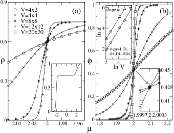
It presents one gas and two liquid, LDL and HDL, phases of densities $\rho=0$, $\rho=3/4$, and $\rho=1$, respectively. For fixed $T$, by increasing $\mu$ we pass through two FOPT, namely, gas-LDL and LDL-HDL.

Figure 1: The ALG model for the parameters as in the text and different $V=L\times L$. The continuous lines are curves from Eq. (1) for: (a) $\rho\times\mu$ around the gas-LDL transition (the inset shows $\rho\times\mu$ in the whole $\mu$ range where the two FOPS take place); and (b) $\phi(=4\rho-3)\times\mu$ around the LDL-HDL transition. The blow up shows the crossing for $L=8,12,20$. The expected linear $a\times V$ behavior is displayed in the inset of (b) (the log-log scale is just for accommodating both cases). For comparison, the simulations for $V=4\times 2$ are exact.

We study the ALG model gas-LDL and LDL-HDL FOPT by plotting the density vs $\mu$ for $T=0.300$, $u=v=1$, and different $V$’s. For the gas-LDL case, we show the results in Fig. 1 (a). We clearly see a good coincident crossing of all curves at $\mu=-1.9986(2)$, for $\rho=0.600(1)$. The exact transition density $\rho=3/5=0.6$ is understood recalling that at the coexistence both gas ($\rho=0$) and LDL ($\rho=3/4$) phases have equal weight. Given that $\alpha_{LDL}=4$, the value follows. Around LDL-HDL, $\rho$ does not vanish, inset of Fig. 1 (a). Since $3/4$ (the totality) of the lattice is filled by molecules in the LDL (HDL) phase, a better order parameter is the rescaled density $\phi=(4\rho-3)$. Thus, in Fig. 1 (b) we display $\phi\times\mu$ for the LDL-HDL transition. Again, all the isotherms are well described by Eq. (1), crossing at $\mu=2.0000(3)$ with $\rho=0.857(1)$. In Fig. 1 (b) inset we confirm the expected linear dependence on $V$ for the parameter $a_{2}=a$ (a single $a$ once we have only two phases in each transition).

Next we consider the Bell-Lavis (BL) model, which also displays water-like anomalies. The sites may or may not be occupied ($\sigma_{\scriptscriptstyle{i}}=$ 1 or 0) by molecules of two possible orientations. But differently from the ALG, the van-der-Waals interaction between two adjacent molecules is attractive, $-\epsilon_{vdw}$. So, there is no energetic punishment if hydrogen bonds (of energy $-\epsilon_{hb}$) are not formed. Such distinctions from the ALG, e.g., result in a second order phase transition for LDL-HDL, but still a FOPS for the gas-LDL. It is described by ($\zeta\equiv\epsilon_{vdw}/\epsilon_{hb}$)

$${\mathcal{H}}=-\epsilon_{hb}\,\sum_{<i,j>}\sigma_{i}\,\sigma_{j}\,[\tau_{i}^{ij}\,\tau_{j}^{ji}+\zeta]-\mu\sum_{i}\sigma_{i}.$$ (3)

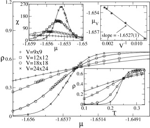
For $\zeta<1/3$, the BL presents three phases, gas ($\rho=0$), LDL ($\rho=2/3$ in a honeycomb structure), and HDL ($\rho=1$) bell . In the numerics we set $\epsilon_{hb}=1$ and $\epsilon_{vdw}=1/10$.

For $T=0.25$, in Fig. 2 we plot $\rho\times\mu$ around the FOPT gas-LDL. Once more, the simulations are well described by Eq. (1). The isotherms cross at $\mu=-1.6528(1)$, with $\rho\approx 0.507(2)$ very close to the exact $\rho=1/2$ (which can be inferred as done for the ALG model). In the upper-left inset we show $\chi=(\frac{\partial\rho}{\partial\mu})_{T}$ by properly differentiating Eq. (1) (continuous lines) and by numerically simulating $\chi=V(\langle\rho^{2}\rangle-\langle\rho\rangle^{2})$. Note the remarkable agreement, again illustrating the power of Eq. (1) to describe relevant thermodynamic quantities around FOPT. The upper-right inset displays the values of $\mu=\mu_{V}$ (for which $\chi$ is maximum) vs $V^{-1}$. This type of scaling extrapolation also can give the thermodynamic limit for the transition, here $\mu=-1.6527$, basically the same value obtained from the crossing. Finally, instead of $\mu$ one could take $T$ as the control parameter. Setting $\mu=-1.6528$ and varying $T$ we see in the lower inset of Fig. 2 the gas-LDL transition. As it should be, the curves cross at $T=0.25$, with $\rho\approx 1/2$. Finally, we note that for $T>0.43$, the results from the present method starts to be less accurate.

Figure 2: For the BL model gas-LDL FOPT and parameters as in the text, $\rho\times\mu$ for distinct $V$’s and $T=0.25$. All the continuous lines are properly obtained from Eq. (1). The upper insets show the isothermal compressibility $\chi$ vs $\mu$ and $\mu_{V}$ (the values of $\mu$ at the peaks of $\chi$) vs $V^{-1}$. The lower inset shows $\rho\times T$ curves for $\mu=-1.6528$, which cross at $T=0.25$.

The Blume-Emery-Griffiths (BEG) model yields BEGMODEL

$${\cal H}=-\sum_{<i,j>}[J\sigma_{i}\,\sigma_{j}+K\sigma_{i}^{2}\sigma_{j}^{2}]-\sum_{i}[H\sigma_{i}-D\sigma_{i}^{2}],$$ (4)

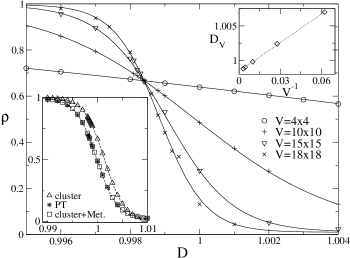
where a site $i$ is either empty or occupied by two different type of species ($\sigma_{i}=0,\pm 1$). Parameters $J$ and $K$ are interaction energies and $D$ and $H$ denote linear combination of the species $\mu$’s. This system is a particularly interesting test because the otherwise very reliable cluster algorithm for the BEG model bouabci fails for some particular $K/J$’s, e.g., the value we address $K/J=-0.5$. So, for a better comparison with our procedure, we also propose a new cluster-Metropolis hybrid approach, which includes intermediary Metropolis algorithm steps (details will appear elsewhere). We note, nevertheless, that the Metropolis alone is not able to cross the high free energy barriers at the phases coexistence.

Figure 3: For the BEG model, $\rho\times\mu$ for parameters as in the text and distinct $V$’s. The results for $V=4\times 4$ are exact. The continuous lines properly come from Eq. (1). The right inset shows $D_{V}$ ($D$ for which $\chi$ is maximum) vs $V^{-1}$. The left inset compares numerical simulations from the PT, cluster and hybrid cluster-Metropolis algorithms for $V=10\times 10$.

In Fig. 3 we plot $\rho\times D$ for $H=0$, $J=1$, $K=-0.5$, $T=0.20$, and different $V$’s. We have a FOPT with all the isotherms crossing at $D=0.9984(1)$ and $\rho\approx 2/3$. The right inset of Fig. 3 shows the position $D_{V}$ of the peak of $\chi=-(\frac{\partial\rho}{\partial D})_{T}$, calculated directly from Eq. (1). A linear extrapolation of $D_{V}\times V^{-1}$ gives $D=0.99845(5)$, in excellent agreement with the crossing value. For $V=10\times 10$, we plot in the left inset simulations from the usual cluster, the improved (but dedicated) cluster-Metropolis, and PT algorithms. The latter two display very good concordance, with the cluster given poorer results. We should mention that for the BEG and ALG models there are no precise simulations in the literature for the parameter conditions here considered.

Lastly, we discuss the asymmetric Ising Hamiltonian on a triangular lattice (of sublattices $(\alpha,\beta,\gamma)$) landau86

$${\cal H}=-J\sum_{<i,j>}\sigma_{i}\sigma_{j}-K\sum_{<i,j,k>}\sigma_{i}\sigma_{j}\sigma_{k}-H\sum_{i}\sigma_{i}.$$ (5)

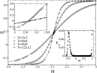
The second sum is over first neighbors trios forming triangles. Using the Wang-Landau method wang , the model has been studied in details wang2 (but for larger systems and lower numerical precision). It displays one ferrimagnetic, $(--+)$, and two ferromagnetic, $(+++)$ and $(---)$, phases. For very low temperatures, by increasing $H$ the system displays a second-order phase transition $(---)\rightarrow(--+)$ and then a FOPT $(--+)\rightarrow(+++)$. The $(--+)$ phase disappears in a critical endpoint ($T_{c}=2.443(1),H_{c}=-2.934(1)$), above it giving rise only to a FOPT between the two ferromagnetic phases. Although the magnetization per site $m$ is not the actual order parameter, for rather small system sizes we can extract from it any relevant FOPT information.

In Fig. 4 we plot $m\times H$ for $J=1,K=2$ and $T=5.00$ for the $(---)\rightarrow(+++)$ FOPT. We see that Eq. (1) represents quite well the transition. In the right inset we show the histogram magnetization density probability $P_{m}$ vs $m$ for $L=12$, $T=5.00$ and $H=-2.3325$, illustrating further that the phases coexistence is being properly characterized fiore-luz-1 . Likewise, the FOPT $(--+)\rightarrow(+++)$ for $T=2.40$ in the left inset is well described by our method. All the isotherms cross at $H=-2.2863(5)$ and $H=-2.9357(5)$ (left inset), in fair agreement (given the different numerical accuracies) with the estimates $H=-2.284(1)$ and $H=-2.939(1)$ by the authors of Ref. wang2 (private communication).

Figure 4: For the asymmetric Ising model and parameters as in the text, $m\times H$ for distinct $V$’s and $T=5.00$ ($T=2.40$, left inset). Continuous lines are the curves from Eq. (1). The right inset shows $P_{m}\times m$ for the $T=5.00$ case.

By considering Eq. (1), derived from rigorous results at low $T$’s, we have proposed a general protocol to study FOPT. It is accurate and demands only few simulations for relatively small systems, hence a computationally low cost procedure. The approach has been very successfully applied to four distinct lattice models. Of course, more analyzes, e.g., for higher dimensions and continuous systems (presently under progress, but with promising preliminary findings) are in order as further tests. Nevertheless, we believe the method already shows itself a valuable tool to analyze the very important problem of FOPT at low temperatures.

Research grants are provided by CNPq and CT-Infra.

References

- (1) S. Koch, Dynamics of first order phase transitions in equilibrium and nonequilibrium systems, Lectures Notes in Physics 207 (Springer-Verlag, New York, 1984); R. E. Kunz, Dynamics of first-order phase transitions in mesoscopic and macroscopic equilibrium and nonequilibrium systems (H. Deutsch Verlag, Frankfurt, 1995).
- (2) J. L. Lebowitz, Rev. Mod. Phys. 71, S346 (1999).
- (3) A. R. Oganov and S. Ono, Nature 430, 445 (2004); C. Matyska and D. A. Yuen, Earth Planet. Sci. Lett. 234, 71 (2005).
- (4) H. Kuwahara, Y. Tomioka, A. Asamitsu, Y. Moritomo, and Y. Tokura, Science 270, 961 (1995).
- (5) I. F. Silvera and J. Tempere, Phys. Rev. Lett. 100, 117602 (2008).
- (6) W. Janke, in Computer Simulations of Surfaces and Interfaces, edited by B. D?nweg, D.P. Landau, and A.I. Milchev, NATO Science Series II: Mathematics, Physics and Chemistry 114 (Kluwer, Dordrecht, 2003), pp. 111-135.
- (7) C. E. Pfister, Ensaios Matematicos 9, 1 (2005).
- (8) M. B. Bouabci and C. E. I. Carneiro, Phys. Rev. B 54, 359 (1996); A. Rachadi and A. Benyoussef, Phys. Rev. B 68, 064113 (2003).
- (9) B. A. Berg and T. Neuhaus, Phys. Lett. B 267, 249 (1991); ibid, Phys. Rev. Lett. 68, 9 (1992).
- (10) F. Wang and D. P. Landau, Phys. Rev. Lett. 86, 2050 (2001).
- (11) C. J. Silva, A. A. Caparica, and J. A. Plascak, Phys. Rev. E 73, 036702 (2006); J. Yin and D. P. Landau, Phys. Rev. E 80, 051117 (2009).
- (12) Y. Okamoto, J. Mol. Graph. and Modelling 22, 425 (2004).
- (13) C. E. Fiore and C. E. I. Carneiro, Phys. Rev. E 76, 021118 (2007).
- (14) C. E. Fiore and M. G. E. da Luz, Phys. Rev. E 82, 031104 (2010)
- (15) C. E. Fiore and M. G. E. da Luz, J. Chem. Phys. 133, 244102 (2010).
- (16) C. Borgs and R. Kotecký, J. Stat. Phys. 61, 79 (1990); ibid, Phys. Rev. Lett. 68, 1734 (1992).
- (17) For the details about the analyticity of the ’s see rBoKo .
- (18) W. Janke, Phys. Rev. B 47, 14757 (1993).
- (19) K. Hukushima and K. Nemoto, J. Phys. Soc. Jpn. 65, 1604 (1996); C. J. Geyer, in Computing Science and Statistics: Proceedings of the 23rd Symposium on the Interface, eds. J. R. Kettenring and E. M. Keramidas, (1991) pp. 156-163.
- (20) E. Marinari and G. Parisi, Europhys. Lett. 19, 451 (1992).
- (21) G. M. Bell and D. A. Lavis, J. Phys. A 3, 568 (1970); C. E. Fiore, M. M. Szortyka, M. C. Barbosa, and V. B. Henriques, J. Chem. Phys 131, 164506 (2009).
- (22) A. L. Balladares, V. B. Henriques, and M. C. Barbosa, J. Phys. C 19, 116105 (2007).
- (23) V. B. Henriques and M. C. Barbosa, Phys. Rev. E 71, 031504 (2005).
- (24) M. Blume, V. J. Emery, and R. B. Griffiths, Phys. Rev. A 4, 1071 (1971); W. Hoston and A. N. Berker, Phys. Rev. Lett. 67, 1027 (1991).
- (25) K. K. Chin and D. P. Landau, Phys. Rev. B 36, 275 (1987).
- (26) S. Tsai, F. Wang and D. P. Landau, Phys. Rev. E 75, 061108 (2007).