HU-EP-11/55
SFB/CPP-11-71
Three-Loop Calculation of the Higgs Boson Mass in
Supersymmetry
Abstract
A Key feature of the minimal supersymmetric extension of the Standard Model (mssm) is the existence of a light Higgs boson, the mass of which is not a free parameter but an observable that can be predicted from the theory. Given that the lhc is able to measure the mass of a light Higgs with very good accuracy, a lot of effort has been put into a precise theoretical prediction.
We present a calculation of the susy-qcd corrections to this observable to three-loop order. We perform multiple asymptotic expansions in order to deal with the multi-scale three-loop diagrams, making heavy use of computer algebra and keeping a keen eye on the numerical error introduced.
We provide a computer code in the form of a Mathematica package that combines our three-loop susy-qcd calculation with the literature of one- and two-loop corrections to the Higgs mass, providing a state-of-the-art prediction for this important observable.
1 Introduction
The minimal supersymmetric extension of the Standard Model (mssm) is a promising candidate for physics beyond the Standard Model. Its Higgs sector is a two-Higgs doublet model with the additional constraint that supersymmetry relates the quartic Higgs couplings to the gauge couplings of the theory. This increases the predictiveness of the model and allows the Higgs sector to be parametrised by just two new parameters, the mass of the pseudoscalar Higgs and the ratio of the vacuum expectation values of the Higgs doublets.
In particular, the mass of the light Higgs boson is not a free parameter, but can be predicted. At tree level, is bounded above by , but radiative corrections shift the value significantly. Since will be a precision observable once the Higgs is found at the Large Hadron Collider (lhc), it is imperative to have a precise theoretical prediction. Consequently, a lot of effort has been put into the calculation of radiative corrections to at the one- and two-loop level (see, for example [1, 2, 3, 4, 5, 6, 7, 8]). The remaining theoretical uncertainty has been estimated to be about GeV [9, 10], which is confirmed by a study of the leading and next-to-leading terms in , where is the typical scale of susy particle masses, at three-loop order [11].
This uncertainty of the theoretical prediction justifies a calculation of the next term in the perturbative expansion. A study of the corrections to shows that the contributions from loops of top quarks and their superpartners, the stops, are dominant at the one- and two-loop level. In [12, 13], we have calculated three-loop susy-qcd corrections to these diagrams. The calculation of these terms is the subject of this talk.
2 Calculation of the Three-Loop Corrections
Motivated by the discussion above, we restrict the calculation at the three-loop level to the susy-qcd corrections where the Higgs couples to a top quark or its superpartners. In the perturbative expansion of , these are the terms of , where is the strong coupling and denotes the coupling of the Higgs to the top quark.
We thus have to evaluate three-loop propagator diagrams in susy-qcd, which faces us with two complications. First, we need a convenient regulator that respects supersymmetry, and second, a lot of masses appear in our diagrams.
2.1 Regularisation by Dimensional Reduction
The regularisation workhorse of multi-loop calculations is dimensional regularisation (dreg) [14], where the number of spacetime dimensions is altered from to , and the divergences of the loop integrals are manifest as poles in .
Unfortunately, dreg does not respect supersymmetry. An easy way to see this is that changing the number of spacetime dimensions also changes the number of degrees of freedoms of the vector fields, and supersymmetry requires an equal number of bosonic and fermionic degrees of freedom. While it is possible (but tedious) to manually construct finite counterterms that restore the supersymmetric ward identities, a more convenient approach was suggested by Siegel under the name of dimensional reduction (dred) [15]. The main idea is that the change of dimensions need only affect momenta in order to regularise the loop integrals. In dred, one splits the four dimensional space into orthogonal spaces of dimension and , and restricts the loop momenta to the dimensional subspace while all gauge fields are kept four dimensional. The components of the gauge fields transform as a tuple of scalar fields and are called -scalars.
The consistent formulation of dred is more involved than sketched here [16], and the question whether the inclusion of the -scalars truly restores the supersymmetric ward identities in all cases is not yet resolved. However, dred has successfully been applied in many multi-loop calculations[17, 18, 19, 20, 21, 22, 23, 24, 25, 26], so far without observing a violation of the ward identities.
2.2 Asymptotic Expansion in the Masses
The difficulty of calculating a Feynman diagram rises with the number of loops, the number of external momenta and the number of masses in the diagram. To obtain the terms of , we have to evaluate diagrams with three loops, two legs and a lot of masses: treating the light quarks as massless and their superpartners as mass degenerate with mass , we are left with five masses: the top quark mass , the masses of its superpartners , , the mass of the gluino and . Calculating these diagrams without any approximations is not feasible with contemporary methods.
Given the mild dependence of the one-loop corrections to on the external momentum, it is reasonable to expand the diagrams in small external momentum, reducing the problem to the evaluation of vacuum diagrams. A further simplification is possible by performing nested asymptotic expansions [27, 28, 29, 30], which expresses the multi-mass diagrams as a series in ratios of the masses and logarithms of these ratios. The coefficients in the series involve only one-scale integrals. Assuming that the ratios of the masses are small, the series should give good approximations to the original diagrams.
Of course, before carrying out the asymptotic expansions, one has to identify which mass ratios are small. Given that so far none of the superpartner masses are known, this is an undecidable problem. So, instead of calculating with a fixed, known, hierarchy among the masses, one has to systematically consider various possible mass hierarchies and carry out the calculation for each of these. To get a prediction of for a specific point in the parameter space of the mssm, where the masses of the superpartners have specific values, one has to choose whichever hierarchy fits these values best.
We carry out the calculation using the following setup: In a first step, all diagrams contributing to at are found using the program qgraf [31]. There are diagrams. For each hierarchy, these diagrams are expanded asymptotically using q2e/exp [32]. The one-scale integrals are then calculated using the form [33] program matad [34].
2.3 Renormalisation
For the renormalisation of the parameters entering our calculation, we adopt a variation of the -scheme, i.e. minimal subtraction using dimensional reduction. This leads to a much better behaviour of the perturbative series compared to using on-shell renormalisation (see Fig. 1).

3 Computer Code
In order to provide a precise prediction for the value of within the mssm, our terms have to be combined with the wealth of corrections from other sectors of the mssm at one- and two-loop level that are available in the literature [1, 2, 3, 4, 5, 6, 7, 8]. Also, the choice of hierarchy mentioned in 2.2 should be automatised. In [13], we have presented the Mathematica package H3m, which is publicly available, to address these points. For convenience, it implements the Susy Les Houches Accord slha [35] and has an interface to the spectrum generators softsusy [36], SuSpect [37] and SPheno [38].
The program uses FeynHiggs [39, 9] to get a two-loop approximation of . An obstacle for adding our terms of to the result delivered by FeynHiggs is the usage of on-shell renormalisation in FeynHiggs. In order to be consistent, we have to convert the and terms that contain on-shell parameters to the scheme. Thanks to [7], which gives a compact expression for these terms both in the and in the on-shell scheme, this obstacle is easily overcome.
The corrections to depend very strongly on the mass of the top quark and the strong coupling . These parameters must be known, within susy-qcd renormalised in the scheme, as precisely as possible. In [40], the relation between the top mass in the - and the on-shell scheme in susy-qcd has been calculated to . Using the library tsil [41], this relation can be used to obtain from the known value of the top quark pole mass.
We determine in susy-qcd from the value of in five-flavour qcd at the mass following [42] by running, within five-flavour qcd, to the decoupling scale where we perform the transition to the full theory. We then run, within susy-qcd, to the desired value of the renormalisation scale.
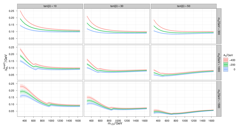
In order to choose the most appropriate hierarchy and get an estimate for the error introduced by the asymptotic expansion, we compute an approximation to the two-loop corrections of using asymptotic expansions in the mass ratios and compare this approximation to the result of [7]. The hierarchy that matches the exact two-loop result best is chosen for the calculation of the three-loop term, and the error at two-loop level is recorded to get a handle on the error in the three-loop result (see Fig. 4).
4 Numerical Results
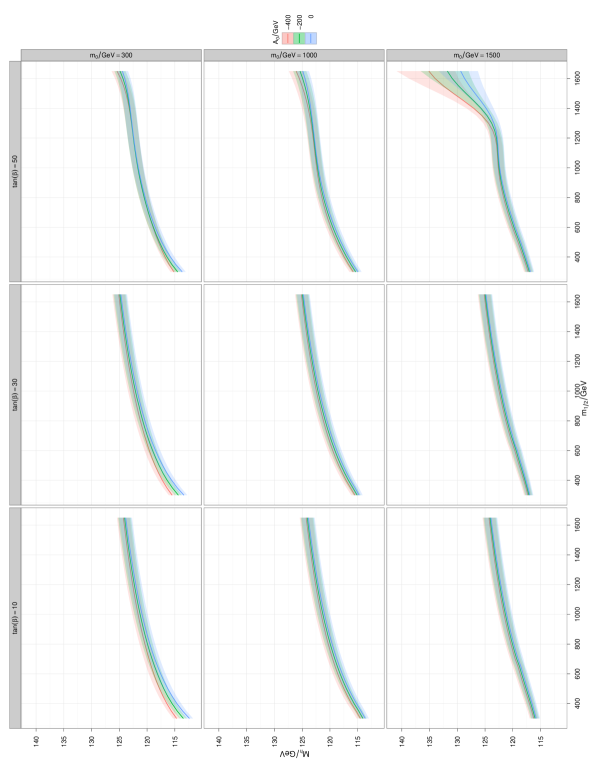
In this chapter, we present a state-of-the-art numerical prediction for in the msugra model that has been obtained with H3m. Fig. 2 shows the dependence of on the parameters , , , and for . The shaded bands around the individual curve show the variation of when is varied between GeV and GeV. We restrict the plot to values of GeV in light of the latest exclusions from the lhc experiments [43, 44, 45, 46].
We observe that of all msugra parameters, varying has by far the largest impact on the Higgs mass. We also observe that the present uncertainty of the top mass directly translates to a parametric uncertainty of about one GeV of the Higgs mass.

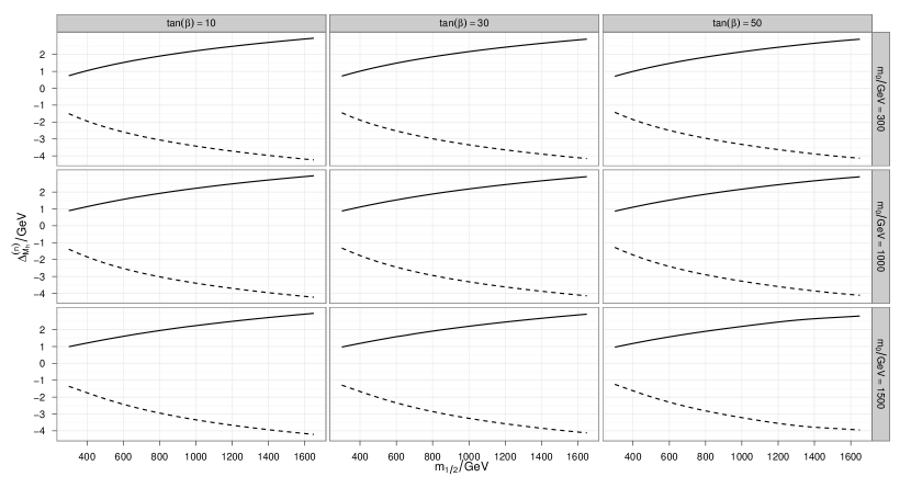
To estimate the effect of unknown higher orders, Fig. 3 shows the two- and three-loop corrections to . We observe a partial cancellation between the two- and three-loop correction. We also observe that while the higher order corrections do decrease in magnitude, they do not do so by a large factor. Thus, we should be careful when estimating the magnitude of the missing higher order contributions. We choose to assign % of the three-loop contribution as a theoretical error. This amounts to a hundred MeV for low values of and to about one GeV for above one GeV. Using the scale variation as an error estimate would lead to a smaller error [13].

By performing asymptotic expansions, we have introduced an additional source of uncertainty to the prediction of . With Fig. 4, we can analyse how large this uncertainty is. It shows the error that we would have introduced had we made the same approximation at the two-loop level. We see that this error is typically at or below MeV, or MeV for low values of and . Since the three-loop corrections are smaller than the two-loop corrections, we expect the actual error due to asymptotic expansions to be below MeV.

5 Conclusions
We have presented a calculation of the corrections to the mass of the light Higgs boson in the mssm. These contributions shift the value of by GeV, depending on the mass spectrum of the superpartners.
The results have been implemented in the program H3m, which is freely available [13].
Using our results, we improve the theoretical error significantly. The theoretical error is now on the order of about MeV for light and GeV for heavy superpartner masses. This is comparable to the parametric uncertainty with the top mass and .
6 Acknowledgements
This work was supported by the DFG through SFB/TR-9 and by the Helmholtz Alliance “Physics at the Terascale”. We thank Robert Harlander, Luminita Mihaila and Matthias Steinhauser, with whom this work was done, Pietro Slavich and Steve Martin for providing us with private code that implements results from [7] and [40], respectively, and Thomas Hahn for useful discussions about some technical details of FeynHiggs.
References
References
- [1] Hempfling R and Hoang A H 1994 Phys. Lett. B331 99–106 (Preprint hep-ph/9401219) \nonumHaber H E, Hempfling R and Hoang A H 1997 Z. Phys. C75 539–554 (Preprint hep-ph/9609331)
- [2] Zhang R 1999 Phys. Lett. B447 89–97 (Preprint hep-ph/9808299)
- [3] Heinemeyer S, Hollik W and Weiglein G 1998 Phys. Rev. D58 091701 (Preprint hep-ph/9803277)
- [4] Pilaftsis A and Wagner C E M 1999 Nucl. Phys. B553 3–42 (Preprint hep-ph/9902371)
- [5] Carena M S et al. 2000 Nucl. Phys. B580 29–57 (Preprint hep-ph/0001002)
- [6] Espinosa J R and Navarro I 2001 Nucl. Phys. B615 82–116 (Preprint hep-ph/0104047)
- [7] Degrassi G, Slavich P and Zwirner F 2001 Nucl. Phys. B611 403–422 (Preprint hep-ph/0105096)
- [8] Martin S P 2003 Phys. Rev. D67 095012 (Preprint hep-ph/0211366)
- [9] Degrassi G, Heinemeyer S, Hollik W, Slavich P and Weiglein G 2003 Eur. Phys. J. C28 133–143 (Preprint hep-ph/0212020)
- [10] Allanach B, Djouadi A, Kneur J, Porod W and Slavich P 2004 JHEP 0409 044 (Preprint hep-ph/0406166)
- [11] Martin S P 2007 Phys. Rev. D75 055005 (Preprint hep-ph/0701051)
- [12] Harlander R V, Kant P, Mihaila L and Steinhauser M 2008 Phys. Rev. Lett. 100 191602 (Preprint 0803.0672)
- [13] Kant P, Harlander R V, Mihaila L and Steinhauser M 2010 JHEP 08 104 (Preprint 1005.5709)
- [14] Wilson K G 1973 Phys. Rev. D7 2911–2926 \nonum’t Hooft G and Veltman M J G 1972 Nucl. Phys. B44 189–213 \nonumBreitenlohner P and Maison D 1977 Commun. Math. Phys. 52 11–38
- [15] Siegel W 1979 Phys. Lett. B84 193
- [16] Stöckinger D 2005 JHEP 03 076 (Preprint hep-ph/0503129)
- [17] Harlander R V, Jones D R T, Kant P, Mihaila L and Steinhauser M 2006 JHEP 12 024 (Preprint hep-ph/0610206)
- [18] Marquard P, Mihaila L, Piclum J and Steinhauser M 2007 Nucl.Phys. B773 1–18 (Preprint hep-ph/0702185)
- [19] Bednyakov A 2007 Int.J.Mod.Phys. A22 5245–5277 (Preprint 0707.0650)
- [20] Jack I, Jones D R T, Kant P and Mihaila L 2007 JHEP 09 058 (Preprint 0707.3055)
- [21] Signer A and Stockinger D 2009 Nucl.Phys. B808 88–120 (Preprint 0807.4424)
- [22] Mihaila L 2009 Phys.Lett. B681 52–59 (Preprint 0908.3403)
- [23] Pak A, Steinhauser M and Zerf N 2011 Eur.Phys.J. C71 1602 (Preprint 1012.0639)
- [24] Harlander R V, Hofmann F and Mantler H 2011 JHEP 1102 055 (Preprint 1012.3361)
- [25] Kilgore W B 2011 Phys.Rev. D83 114005 (Preprint 1102.5353)
- [26] Hermann T, Mihaila L and Steinhauser M 2011 Phys.Lett. B703 51–59 (Preprint 1106.1060)
- [27] Tkachov F V 1993 Int. J. Mod. Phys. A8 2047–2117 (Preprint hep-ph/9612284) \nonumPivovarov G B and Tkachov F V 1993 Int. J. Mod. Phys. A8 2241–2286 (Preprint hep-ph/9612287)
- [28] Gorishnii S G and Larin S A 1987 Nucl. Phys. B283 452
- [29] Smirnov V A and Chetyrkin K G In Alushta 1987, Proceedings, Problems of quantum field theory 48-53. \nonumChetyrkin K G MPI-PH-91-13
- [30] Smirnov V A 1990 Commun. Math. Phys. 134 109–137 \nonumSmirnov V A Basel, Switzerland: Birkhaeuser (1991) 380 p. (Progress in physics, 14)
- [31] Nogueira P 1993 J. Comput. Phys. 105 279–289
- [32] Seidensticker T 1999 (Preprint hep-ph/9905298) \nonumHarlander R, Seidensticker T and Steinhauser M 1998 Phys. Lett. B426 125–132 (Preprint hep-ph/9712228)
- [33] Vermaseren J A M 2000 (Preprint math-ph/0010025)
- [34] Steinhauser M 2001 Comput. Phys. Commun. 134 335–364 (Preprint hep-ph/0009029)
- [35] Skands P Z et al. 2004 JHEP 07 036 (Preprint hep-ph/0311123)
- [36] Allanach B 2002 Comput.Phys.Commun. 143 305–331 (Preprint hep-ph/0104145)
- [37] Djouadi A, Kneur J L and Moultaka G 2007 Comput.Phys.Commun. 176 426–455 (Preprint hep-ph/0211331)
- [38] Porod W and Staub F 2011 (Preprint 1104.1573) \nonumPorod W 2003 Comput.Phys.Commun. 153 275–315 (Preprint hep-ph/0301101)
- [39] Heinemeyer S, Hollik W, Weiglein G 2000 Comput. Phys. Commun. 124 76–89 (Preprint hep-ph/9812320) \nonumHeinemeyer S, Hollik W and Weiglein G 1999 Eur. Phys. J. C9 343–366 (Preprint hep-ph/9812472) \nonumFrank M et al. 2007 JHEP 02 047 (Preprint hep-ph/0611326)
- [40] Martin S P 2005 Phys. Rev. D72 096008 (Preprint hep-ph/0509115)
- [41] Martin S P and Robertson D G 2006 Comput. Phys. Commun. 174 133–151 (Preprint hep-ph/0501132)
- [42] Harlander R V, Mihaila L and Steinhauser M 2007 Phys. Rev. D76 055002 (Preprint 0706.2953)
- [43] Atlas Collaboration 2011 (Preprint 1110.2299)
- [44] ATLAS Collaboration 2011 Phys.Rev.D (Preprint 1109.6606)
- [45] Padhi S (for the CMS Collaboration) 2011 (Preprint 1111.2733)
- [46] Schettler H (for the CMS Collaboration) 2011 (Preprint 1111.2256)