Implications of Family Nonuniversal $Z^{\prime}$ Model on $B\to K_{0}^{*}\pi$ Decays

Abstract

Within the QCD factorization formalism, we study the possible impacts of the nonuniversal $Z^{\prime}$ model, which provides a flavor-changing neutral current at the tree level, on rare decays $B\to K_{0}^{*}\pi$. Under two different scenarios (S1 and S2) for identifying the scalar meson $K_{0}^{*}(1430)$, the branching ratios, $CP$ asymmetries, and isospin asymmetries are calculated in both the standard model (SM) and the family nonuniversal $Z^{\prime}$ model. We find that the branching ratios and $CP$ asymmetries are sensitive to weak annihilation. In the SM, with $\rho_{A}=1$ and $\phi_{A}\in[-30^{\circ},30^{\circ}]$, the branching ratios of S1 (S2) are smaller (larger) than the experimental data. Adding the contribution of the $Z^{\prime}$ boson in two different cases (Case-I and Case-II), for S1, the branching ratios are still far away from experiment. For S2, in Case-II, the branching ratios become smaller and can accommodate the data; in Case-I, although the center values are enhanced, they can also explain the data with large uncertainties. Similar conclusions are also reached for $CP$ asymmetries. Our results indicate that S2 is more favored than S1, even after considering new physics effects. Moreover, if there exists a nonuniversal $Z^{\prime}$ boson, Case-II is preferred. All results can be tested in the LHC-b experiment and forthcoming super-B factory.

I Introduction

Recently, with rich events in two $B$ factories, measurements of $B$ meson nonleptonic charmless decays involving scalar mesons have become available. Among these decays, the processes $B\to K_{0}^{*}\pi$ are attractive since they are dominantly induced by the flavor-changing neutral current (FCNC) transition $b\to s\bar{q}q~{}(q=u,d,s)$. Such a transition forbidden at the tree level in the Standard Model (SM) is expected to be an excellent ground for testing SM and searching for new physics (NP) beyond SM. Therefore, many similar decay modes induced by FCNC have been explored widely in the literatures, such as $B\to K\pi,K\eta^{(\prime)},\phi K^{(*)}$. The recent reviews can be found, for example, in Ref. Cheng:2010yv . For the concerned decay modes $B\to K_{0}^{*}\pi$, the latest world averaged branching ratios from Heavy Flavor Average Group Asner:2010qj are listed as:

$${BR}(B^{+}\to K^{*0}_{0}(1430)\pi^{+}) = (45.1\pm 6.3)\times 10^{-6};$$

$${BR}(B^{0}\to K^{*+}_{0}(1430)\pi^{-}) = (33.5^{+3.9}_{-3.8})\times 10^{-6};$$

$${BR}(B^{0}\to K^{*0}_{0}(1430)\pi^{0}) = (11.7^{+4.2}_{-3.8})\times 10^{-6}.$$ (1)

Direct $CP$ asymmetries of above decays have also been measured recently by BaBar and Belle experiments, which will be shown in Sec. IV. As direct $CP$ violation is sensitive to the strong phase involved in the decay process, the comparison between theory and experiment will offer us information on the strong phases necessary for producing the measured direct $CP$ asymmetries. Comparing the predicted results of the SM Cheng:2005nb with experimental data, ie. Eq.(I), we notice that the theoretical results cannot accommodate the data well even with large uncertainties. So, it is worth while to explore whether some new physics models could explain the data.

When discussing the $B$ meson non-leptonic charmless decays, the hadronic matrix elements are required. In the past few years, several novel methods have been proposed to study matrix elements related to exclusive hadronic $B$ decays, such as naive factorization (NF) Wirbel:1985ji , generalized factorization Ali:1998eb , the perturbative QCD method (pQCD) Lu:2000em , QCD factorization (QCDF) Beneke:1999br , the soft collinear effective theory (SCET) Bauer:2001cu , and so on. Among these approaches, QCDF based on collinear factorization is a systematic framework to compute these matrix elements from QCD theory, and it holds in the heavy quark limit $m_{b}\to\infty$ and the heavy quark symmetry. Thus, we shall use QCDF approach in the following calculations.

Although the study of scalar meson spectrum has been an interesting topic for a long time, the underlying structure of the light scalar meson is still controversial until now. In the literature, there are many schemes for the classification of them. Here we present two typical scenarios to describe the scalar mesons Tornqvist:1982yv . Scenario-1 (S1) is the naive 2-quark model: the nonet mesons below 1 GeV are treated as the lowest lying states, and the ones near 1.5 GeV are the first orbitally excited states. In scenario-2 (S2), the nonet mesons near 1.5 GeV are regarded as the lowest lying states, while the mesons below 1 GeV may be viewed as exotic states beyond the two-quark model. Since the mass of $K^{*}_{0}(1430)$ is very near 1.5 GeV, thus it should be composed by two quarks in both S1 and S2, but the decay constants and distribution amplitudes are different in the different scenarios. Under above pictures, the two body nonleptonic $B$ decays involving scalar mesons have been explored in both QCDF Cheng:2005ye ; Cheng:2005nb ; Cheng:2007st and pQCD approaches Chen:2002si ; Chen:2005cx ; Wang:2006ria ; shen ; Kim:2009dg .

As stated before, $B\to K_{0}^{*}\pi$ decays are dominantly induced by FCNC $b\to s\bar{q}q$ transition, hence they are sensitive to new physics contributions even if they are suppressed by a large mass parameter which characterizes the new physics scale. To search for signals of NP, a model independent analysis is not suitable for the current status. It is the purpose of this work to show that a new physics effect of similar size can be obtained from some models with an extra $Z^{\prime}$ boson. $Z^{\prime}$ bosons are known to naturally exist in certain well-motivated extensions of the SM, such as the string theory String , the grand unified theories GUTs , the little Higgs modelsLH , light U-boson model Uboson , by adding additional $U(1)^{\prime}$ gauge symmetry. Among those models, a well-motivated $Z^{\prime}$ model for low energy systems is the so-called family non-universal $Z^{\prime}$ model, where the $Z^{\prime}$ couplings are affected by fermion mixing and are not diagonal in the mass basis. Non-trivial flavor-changing neutral current (FCNC) effects at the tree level mediated by the $Z^{\prime}$ therefore are induced, which play an important role in explaining the $CP$ asymmetries in the current high energy experiments by introducing new weak phases. The effects of $Z^{\prime}$ boson in $B$ sector have been investigated in a number of papers Langacker:2000ju ; Barger:2009hn ; Cheung:2006tm ; Chang:2009wt ; Langacker:2008yv . In this work, we will show the implications of the family nonuniversal $Z^{\prime}$ model on $B\to K_{0}^{*}\pi$ decays.

The layout of this paper is as follows. In Sec.II, we firstly present the formulaes of $B\to K_{0}^{*}\pi$ in the SM within the QCDF approach, involving the effective Hamiltonian and the amplitudes. In Sec.III, we specify our flavor-changing $Z^{\prime}$ model, and how the effective Hamiltonian responsible for hadronic $B$ decays is modified. The numerical results and discussions are given in Sect.IV.The conclusions are presented in the final section.

II Calculation in the Standard Model

In the two-quark picture of S1 and S2, the two kinds of decay constants of scalar meson $S$ are defined by:

$$\langle S(p)|\bar{q}_{2}\gamma_{\mu}q_{1}|0\rangle=f_{S}p_{\mu},\,\,\,\,\,\,\,\,\,\,\,\langle S(p)|\bar{q}_{2}q_{1}|0\rangle=m_{S}\bar{f_{S}}.$$ (2)

The vector decay constant $f_{S}$ and the scale-dependent scalar decay constant $\bar{f}_{S}$ are related by equations of motion

$$\mu_{S}f_{S}=\bar{f}_{S},\qquad\quad{\rm with}~{}~{}\mu_{S}=\frac{m_{S}}{m_{2}(\mu)-m_{1}(\mu)},$$ (3)

where $m_{2}$ and $m_{1}$ are the running current quark masses. Therefore, contrary to the case of pseudoscalar one, the vector decay constant of the scalar meson, namely, $f_{S}$, will vanish in the SU(3) limit. In other words, the vector decay constant of $K_{0}^{*}(1430)$ is fairly small.

As for the scalar meson wave function, the twist-2 and twist-3 light-cone distribution amplitudes (LCDAs) for different components could be combined into a single matrix element:

$$\langle K_{0}^{*+}(p)|\bar{u}_{\beta}(z)s_{\alpha}(0)|0\rangle=\frac{1}{\sqrt{6}}\int^{1}_{0}dxe^{ixp\cdot z}\bigg{\{}p\!\!\!\!/\phi_{K^{*+}_{0}}(x)+m_{S}\phi^{S}_{K^{*+}_{0}}(x)+\frac{1}{6}m_{S}\sigma_{\mu\nu}p^{\mu}z^{\nu}\phi^{\sigma}_{K^{*+}_{0}}(x)\bigg{\}}_{\alpha\beta}.$$ (4)

The distribution amplitudes $\phi_{K^{*}_{0}}(x)$, $\phi^{S}_{K^{*}_{0}}(x)$, and $\phi^{\sigma}_{K^{*}_{0}}(x)$ are normalized as:

$$\int^{1}_{0}dx\phi_{K^{*}_{0}}(x)=\frac{f_{K^{*}_{0}}}{2\sqrt{6}},\,\,\,\,\,\,\int^{1}_{0}dx\phi^{S}_{K^{*}_{0}}(x)=\int^{1}_{0}dx\phi^{\sigma}_{K^{*}_{0}}(x)=\frac{\bar{f}_{K^{*}_{0}}}{2\sqrt{6}},$$ (5)

and $\phi^{T}_{K^{*}_{0}}(x)=\frac{1}{6}\frac{d}{dx}\phi^{\sigma}_{K^{*}_{0}}(x)$. The twist-2 LCDA can be expanded in the Gegenbauer polynomials:

$$\phi_{S}(x,\mu)=\frac{1}{\sqrt{2N_{c}}}\bar{f}_{S}(\mu)6x(1-x)\sum_{m=1}^{\infty}B_{m}(\mu)C^{3/2}_{m}(2x-1).$$ (6)

The decay constants and the Gegenbauer moments for twist-2 wave function in two different scenarios have been studied explicitly in Ref. Cheng:2005ye ; Cheng:2005nb using the QCD sum rule approach. As for the explicit form of the Gegenbauer moments for the twist-3 wave functions, there exist few drawbacks in the theoretical calculation Lu:2006fr , thus we choice the asymptotic form for simplicity:

$$\phi^{s}_{S}=\frac{1}{\sqrt{2N_{c}}}\bar{f}_{f},\,\,\,\,\,\,\,\,\,\,\,\,\,\,\,\,\,\,\phi_{S}^{T}=\frac{1}{\sqrt{2N_{c}}}\bar{f}_{S}(1-2x).$$ (7)

For the pion meson, the asymptotic forms for twist-2 and twist-3 distribution amplitudes are also adopted:

$$\phi_{P}(x)=f_{P}6x(1-x),\,\,\,\,\,\,\,\,\,\phi_{P}^{p}(x)=f_{P},\,\,\,\,\,\,\,\,\,\phi_{P}^{\sigma}(x)=f_{P}6x(1-x).$$ (8)

The form factors of $B\to P,S$ transitions are defined by Wirbel:1985ji :

$$\langle P(p^{\prime})|V_{\mu}|B(p)\rangle=\left(P_{\mu}-{m_{B}^{2}-m_{P}^{2}\over q^{2}}\,q_{\mu}\right)F_{1}^{BP}(q^{2})+{m_{B}^{2}-m_{P}^{2}\over q^{2}}q_{\mu}\,F_{0}^{BP}(q^{2}),$$

$$\langle S(p^{\prime})|A_{\mu}|B(p)\rangle=-i\Bigg{[}\left(P_{\mu}-{m_{B}^{2}-m_{S}^{2}\over q^{2}}\,q_{\mu}\right)F_{1}^{BS}(q^{2})+{m_{B}^{2}-m_{S}^{2}\over q^{2}}q_{\mu}\,F_{0}^{BS}(q^{2})\Bigg{]},$$ (9)

where $P_{\mu}=(p+p^{\prime})_{\mu}$, $q_{\mu}=(p-p^{\prime})_{\mu}$. Various form factors have been evaluated by utilizing the relativistic covariant light-front quark model CCH . And the momentum dependence is fitted to a 3-parameter form

$$F(q^{2})=\,{F(0)\over 1-a(q^{2}/m_{B}^{2})+b(q^{2}/m_{B}^{2})^{2}}\,.$$ (10)

The parameters $a$ and $b$ relevant for our purposes are refereed to Ref. CCH .

Although we concentrate on the study of new physics, the used notation for new interacting operators will be similar to those presented in the SM. Therefore, it is useful to introduce the effective operators of the SM. Thus, we describe the effective Hamiltonian for $b\to sq\bar{q}$ decays as

$$H_{{\rm eff}}={\frac{G_{F}}{\sqrt{2}}}\sum_{p=u,c}\lambda_{p}\left[C_{1}(\mu)O_{1}^{(q)}(\mu)+C_{2}(\mu)O_{2}^{(q)}(\mu)+\sum_{i=3}^{10}C_{i}(\mu)O_{i}(\mu)\right]\;,$$ (11)

where $\lambda_{q}=V_{qb}V_{qs}^{*}$ are the Cabibbo-Kobayashi-Maskawa (CKM) matrix elements and the operators $O_{1}$-$O_{10}$ are defined as Buchalla

$$O_{1}^{(q)}=(\bar{s}_{\alpha}q_{\beta})_{V-A}(\bar{q}_{\beta}b_{\alpha})_{V-A}\;,\;\;\;\;\;\;\;\;O_{2}^{(q)}=(\bar{s}_{\alpha}q_{\alpha})_{V-A}(\bar{q}_{\beta}b_{\beta})_{V-A}\;,$$

$$O_{3}=(\bar{s}_{\alpha}b_{\alpha})_{V-A}\sum_{q}(\bar{q}_{\beta}q_{\beta})_{V-A}\;,\;\;\;\;O_{4}=(\bar{s}_{\alpha}b_{\beta})_{V-A}\sum_{q}(\bar{q}_{\beta}q_{\alpha})_{V-A}\;,$$

$$O_{5}=(\bar{s}_{\alpha}b_{\alpha})_{V-A}\sum_{q}(\bar{q}_{\beta}q_{\beta})_{V+A}\;,\;\;\;\;O_{6}=(\bar{s}_{\alpha}b_{\beta})_{V-A}\sum_{q}(\bar{q}_{\beta}q_{\alpha})_{V+A}\;,$$

$$O_{7}=\frac{3}{2}(\bar{s}_{\alpha}b_{\alpha})_{V-A}\sum_{q}e_{q}(\bar{q}_{\beta}q_{\beta})_{V+A}\;,\;\;O_{8}=\frac{3}{2}(\bar{s}_{\alpha}b_{\beta})_{V-A}\sum_{q}e_{q}(\bar{q}_{\beta}q_{\alpha})_{V+A}\;,$$

$$O_{9}=\frac{3}{2}(\bar{s}_{\alpha}b_{\alpha})_{V-A}\sum_{q}e_{q}(\bar{q}_{\beta}q_{\beta})_{V-A}\;,\;\;O_{10}=\frac{3}{2}(\bar{s}_{\alpha}b_{\beta})_{V-A}\sum_{q}e_{q}(\bar{q}_{\beta}q_{\alpha})_{V-A}\;,$$ (12)

with $\alpha$ and $\beta$ being the color indices. In Eq.(11), $O_{1}$-$O_{2}$ are from the tree level of weak interactions, $O_{3}$-$O_{6}$ are the so-called QCD penguin operators and $O_{7}$-$O_{10}$ are the electroweak penguin operators, while $C_{1}$-$C_{10}$ are the corresponding Wilson coefficients.

In the QCDF approach, the contribution of the non-perturbative sector is dominated by the form factors and the non-factorizable impact in the hadronic matrix elements is controlled by hard gluon exchange. The hadronic matrix elements of the decay can be written as

$$\langle M_{1}M_{2}|O_{i}|B\rangle=\sum_{j}F_{j}^{B\rightarrow M_{1}}\int_{0}^{1}dxT_{ij}^{I}(x)\Phi_{M_{1}}(x)+\int_{0}^{1}d\xi\int_{0}^{1}dx\int_{0}^{1}dyT_{i}^{II}(\xi,x,y)\Phi_{B}(\xi)\Phi_{M_{1}}(x)\Phi_{M_{2}}(y).$$ (13)

Here $T_{ij}^{I}$ and $T_{i}^{II}$ denote the perturbative short-distance interactions and can be calculated perturbatively. $\Phi_{X}(x)$ are non-perturbative light-cone distribution amplitudes, which should be universal. Using the weak effective Hamiltonian given by Eq.(11) and the definitions of $a_{i}$ and $b_{i}$ in Ref.Beneke:1999br ; Cheng:2005nb , we can now write the decay amplitudes of $B\to K_{0}^{*}\pi$ as:

$$A(B^{-}\to\overline{K}^{*0}_{0}\pi^{-}) = \frac{G_{F}}{\sqrt{2}}\sum_{p=u,c}\lambda_{p}\Bigg{\{}\left(a_{4}^{p}-r_{\chi}^{K^{*}_{0}}a_{6}^{p}-{1\over 2}(a_{10}^{p}-r_{\chi}^{K^{*}_{0}}a_{8}^{p})\right)_{\pi K^{*}_{0}}f_{K_{0}^{*}}F_{0}^{B\pi}(m_{K_{0}^{*}}^{2})(m_{B}^{2}-m_{\pi}^{2})$$ (14)

$$+f_{B}\big{(}b_{2}\delta_{u}^{p}+b_{3}+b_{\rm 3,EW}\big{)}_{\pi K^{*}_{0}}\Bigg{\}},$$

$$A(B^{-}\to K^{*-}_{0}\pi^{0}) = \frac{G_{F}}{2}\sum_{p=u,c}\lambda_{p}\Bigg{\{}\left(a_{1}\delta_{u}^{p}+a_{4}^{p}-r_{\chi}^{K^{*}_{0}}a_{6}^{p}+a_{10}^{p}-r_{\chi}^{K^{*}_{0}}a_{8}^{p}\right)_{\pi K^{*}_{0}}f_{K_{0}^{*}}F_{0}^{B\pi}(m_{K_{0}^{*}}^{2})(m_{B}^{2}-m_{\pi}^{2})$$

$$- \left[a_{2}\delta_{u}^{p}+{3\over 2}(a_{9}-a_{7})\right]_{K^{*}_{0}\pi}f_{\pi}F_{0}^{BK^{*}_{0}}(m_{\pi}^{2})(m_{B}^{2}-m_{K_{0}^{*}}^{2})+f_{B}\big{(}b_{2}\delta_{u}^{p}+b_{3}+b_{\rm 3,EW}\big{)}_{\pi K^{*}_{0}}\Bigg{\}},$$

$$A(\overline{B}^{0}\to K^{*-}_{0}\pi^{+}) = \frac{G_{F}}{\sqrt{2}}\sum_{p=u,c}\lambda_{p}\Bigg{\{}\left(a_{1}\delta_{u}^{p}+a_{4}^{p}-r_{\chi}^{K^{*}_{0}}a_{6}^{p}+a_{10}^{p}-r_{\chi}^{K^{*}_{0}}a_{8}^{p}\right)_{\pi K^{*}_{0}}f_{K_{0}^{*}}F_{0}^{B\pi}(m_{K_{0}^{*}}^{2})(m_{B}^{2}-m_{\pi}^{2})$$ (16)

$$+ f_{B}\big{(}b_{3}-{1\over 2}b_{\rm 3,EW}\big{)}_{\pi K^{*}_{0}}\Bigg{\}},$$

$$A(\overline{B}^{0}\to\overline{K}^{*0}_{0}\pi^{0}) = \frac{G_{F}}{2}\sum_{p=u,c}\lambda_{p}\Bigg{\{}\left(-a_{4}^{p}+r_{\chi}^{K^{*}_{0}}a_{6}^{p}+{1\over 2}(a_{10}^{p}-r_{\chi}^{K^{*}_{0}}a_{8}^{p})\right)_{\pi K^{*}_{0}}f_{K_{0}^{*}}F_{0}^{B\pi}(m_{K_{0}^{*}}^{2})(m_{B}^{2}-m_{\pi}^{2})$$

$$- \left[a_{2}\delta_{u}^{p}+{3\over 2}(a_{9}-a_{7})\right]_{K^{*}_{0}\pi}f_{\pi}F_{0}^{BK^{*}_{0}}(m_{\pi}^{2})(m_{B}^{2}-m_{K_{0}^{*}}^{2})+f_{B}\big{(}-b_{3}+{1\over 2}b_{\rm 3,EW}\big{)}_{\pi K^{*}_{0}}\Bigg{\}},$$

where $\lambda_{p}\equiv V_{pb}V_{ps}^{*}$ and

$$r^{K^{*}_{0}}_{\chi}(\mu)={2m_{K_{0}^{*}}^{2}\over m_{b}(\mu)(m_{s}(\mu)-m_{q}(\mu))}.$$ (18)

In the above formulaes, the order of the arguments of the $a_{i}^{p}(M_{1}M_{2})$ and $b_{i}(M_{1}M_{2})$ coefficients is dictated by the subscript $M_{1}M_{2}$, where $M_{2}$ is the emitted meson and $M_{1}$ shares the same spectator quark with the $B$ meson. For the annihilation diagram, $M_{1}$ is referred to the one containing an anti-quark from the weak vertex, while $M_{2}$ contains a quark from the weak vertex. Note that the coefficients $a_{i}$ come from vertex corrections and hard spectator corrections, and $b_{i}$ represent of contribution of annihilation diagrams. Both $a_{i}$ and $b_{i}$ can be found in Ref.Cheng:2005nb . It must be emphasized that we shall evaluate the vertex corrections to the decay amplitudes at the scale $\mu=m_{b}/2$. In contrast, the hard spectator and annihilation contributions should be evaluated at the hard-collinear scale $\mu_{h}=\sqrt{\mu\Lambda_{h}}$ with $\Lambda_{h}\approx 500$ MeV.

In QCDF approach, the annihilation amplitude has endpoint divergences even at twist-2 level and the hard spectator scattering diagram at twist-3 order is power suppressed and posses soft and collinear divergences arising from the soft spectator quark. Since the treatment of endpoint divergences is model dependent, subleading power corrections generally can be studied only in a phenomenological way. We shall follow Beneke:1999br ; Cheng:2005nb to parameterize the endpoint divergence $X_{A}\equiv\int^{1}_{0}dx/\bar{x}$ in the annihilation diagram as

$$X_{A}=\ln\left({m_{B}\over\Lambda_{h}}\right)(1+\rho_{A}e^{i\phi_{A}}),$$ (19)

with the unknown real parameters $\rho_{A}$ and $\phi_{A}$. Likewise, the endpoint divergence $X_{H}$ in the hard spectator contributions can be parameterized in a similar manner. In the Sec.IV, we will see that such divergence is the main source of the uncertainty for the concerned decay modes.

III The Family Non-universal $Z^{\prime}$ Model

As mentioned before, a family non-universal $Z^{\prime}$ model leads to FCNC at the tree level due to the non-diagonal chiral coupling matrix, which makes itself become interesting in some penguin dominate processes. The basic formalism of flavor changing effects in the $Z^{\prime}$ model with family nonuniversal and/or nondiagonal couplings has been laid out in Refs. Langacker:2000ju ; Langacker:2008yv , to which we refer readers for detail. The detailed phenomenological analysis for various low energy physics, especially for $B$ meson decays, could be found in Refs. Barger:2009hn ; Cheung:2006tm ; Chang:2009wt . Here we just briefly review the ingredients needed in this paper.

In practice, neglecting the renormalization group (RG) running between $m_{W}$ and $m_{Z^{\prime}}$ and mixing between $Z^{\prime}$ and $Z$ boson of the SM, we write the $Z^{\prime}$ term of the neutral-current Lagrangian in the gauge basis as

$${\cal L}=-g^{\prime}J^{\prime}_{\mu}Z^{\prime\mu},$$ (20)

where $g^{\prime}$ is the gauge coupling constant of extra $U(1)^{\prime}$ group at the electro-weak $m_{W}$ scale. The chiral current $J^{\prime}_{\mu}$ is expressed as:

$$J^{\prime}_{\mu}=\bar{\psi}_{i}\gamma_{\mu}\bigg{[}(B_{ij}^{L})P_{L}+(B_{ij}^{R})P_{R}\bigg{]}~{}\psi_{j},$$ (21)

where the chirality projection operators are $P_{L,R}\equiv(1\pm\gamma_{5})/2$ and $B_{ij}^{X}$ refers to the effective $Z^{\prime}$ couplings to the quarks $i$ and $j$ at the electroweak scale. For simplicity, we assume that the right hand couplings are flavor-diagonal and neglect $B_{sb}^{R}$. Compared with Eq.(11), the effective Hamiltonian for $b\to s\bar{q}q$ transition with $Z^{\prime}$ boson can be written as

$${\cal H}_{\rm eff}^{\rm Z^{\prime}}=\frac{2G_{F}}{\sqrt{2}}\big{(}\frac{g^{\prime}m_{Z}}{g_{1}m_{Z^{\prime}}}\big{)}^{2}\,B_{sb}^{L}(\bar{s}b)_{V-A}\sum_{q}\big{[}B_{qq}^{L}(\bar{q}q)_{V-A}+B_{qq}^{R}(\bar{q}q)_{V+A}\big{]}+{\rm h.c.}\,,$$ (22)

where $m_{Z^{\prime}}$ is the mass of the new gauge boson. In fact, the forms of four-quark operators in Eq. (22) already exist in the SM, so we rewrite it as

$${\cal H}_{\rm eff}^{\rm Z^{\prime}}=-\frac{G_{F}}{\sqrt{2}}V_{tb}V_{ts}^{\ast}\sum_{q}\big{(}\Delta C_{3}O_{3}^{q}+\Delta C_{5}O_{5}^{q}+\Delta C_{7}O_{7}^{q}+\Delta C_{9}O_{9}^{q}\big{)}+{\rm h.c.}\,,$$ (23)

where $O_{i}^{q}~{}(i=3,5,7,9)$ are the effective four-quark operators in the SM. $\Delta C_{i}$ denote the modifications to the corresponding SM Wilson coefficients, which are expressed as

$$\Delta C_{3,5} = -\frac{2}{3V_{tb}V_{ts}^{\ast}}\,\big{(}\frac{g^{\prime}m_{Z}}{g_{1}m_{Z^{\prime}}}\big{)}^{2}\,B_{sb}^{L}\,(B_{uu}^{L,R}+2B_{dd}^{L,R})\,,$$

$$\Delta C_{9,7} = -\frac{4}{3V_{tb}V_{ts}^{\ast}}\,\big{(}\frac{g^{\prime}m_{Z}}{g_{1}m_{Z^{\prime}}}\big{)}^{2}\,B_{sb}^{L}\,(B_{uu}^{L,R}-B_{dd}^{L,R})\,,$$ (24)

Generally, the diagonal elements of the effective coupling matrices $B_{qq}^{L,R}$ are expected to be real as a consequence of the hermiticity of the effective weak Hamiltonian. However, the off-diagonal one $B_{sb}$ perhaps contains a new weak phase $\phi_{s}$. We also suppose $B_{qq}^{L}=B_{qq}^{R}=B_{qq}$, so as to reduce the new parameters. For convenience we can represent $\Delta C_{i}$ as

$$\Delta C_{3,5}=2\,\frac{|V_{tb}V_{ts}^{\ast}|}{V_{tb}V_{ts}^{\ast}}\,\zeta\,e^{i\phi_{s}}\,,\quad\Delta C_{9,7}=4\,\frac{|V_{tb}V_{ts}^{\ast}|}{V_{tb}V_{ts}^{\ast}}\,\xi\,e^{i\phi_{s}}\,,$$ (25)

where $\zeta$ and $\xi$ are defined, respectively, as

$$\zeta = -\frac{1}{3}\,\big{(}\frac{g^{\prime}M_{Z}}{g_{1}M_{Z^{\prime}}}\big{)}^{2}\,\big{|}\frac{B_{sb}^{L}}{V_{tb}V_{ts}^{\ast}}\big{|}\,(B_{uu}+2B_{dd}),$$

$$\xi = -\frac{1}{3}\,\big{(}\frac{g^{\prime}M_{Z}}{g_{1}M_{Z^{\prime}}}\big{)}^{2}\,\big{|}\frac{B_{sb}^{L}}{V_{tb}V_{ts}^{\ast}}\big{|}\,(B_{uu}-B_{dd}).$$ (26)

It is stressed that the other SM Wilson coefficients may also receive contributions from the $Z^{\prime}$ boson through renormalization group (RG) evolution. With our assumption that no significant RG running effect between $M_{Z}^{\prime}$ and $M_{W}$ scales, the RG evolution of the modified Wilson coefficients is exactly the same as the ones in the SM Buchalla .

In order to show the effects of $Z^{\prime}$ boson clearly, our analysis are divided into the two cases with two different simplifications,

$$\left\{\begin{array}[]{llll}B_{uu}=-2B_{dd},&\zeta=0,&\xi=X,&\hbox{Case I;}\\ B_{uu}=B_{dd},&\zeta=-X,&\xi=0,&\hbox{Case II.}\end{array}\right.$$ (29)

with

$$X=\big{(}\frac{g^{\prime}M_{Z}}{g_{1}M_{Z^{\prime}}}\big{)}^{2}\,\left|\frac{B_{sb}^{L}B_{dd}}{V_{tb}V_{ts}^{\ast}}\right|=y\left|\frac{B_{sb}^{L}B_{dd}}{V_{tb}V_{ts}^{\ast}}\right|\,.$$ (30)

Thus, there are only two parameters, $X$ and weak phase $\phi_{s}$ left, in the sequential numerical calculations and discussions.

IV Numerical Results and Discussions

To obtain the numerical results, we list the parameters related to the SM firstly. As stated in Section. I, because we have not a clear conclusion whether $K_{0}^{*}(1430)$ belongs to the first orbitally excited state (S1) or the low lying state (S2), we have to calculate the processes under both scenarios. So, the decay constants, Gegenbauer moments, and form factors in different scenarios are listed as follows Cheng:2005nb :

$$\mathbf{S1}:\bar{f}_{K_{0}^{*}}(1.0~{}~{}\mathrm{GeV})=-300~{}~{}\mathrm{MeV};\bar{f}_{K_{0}^{*}}(2.1~{}~{}\mathrm{GeV})=-370~{}~{}\mathrm{MeV};B_{1}(1.0~{}~{}\mathrm{GeV})=0.58;$$

$$B_{1}(2.1~{}~{}\mathrm{GeV})=0.39;B_{3}(1.0~{}~{}\mathrm{GeV})=-1.20;B_{3}(2.1~{}~{}\mathrm{GeV})=-0.70;F_{0}^{BK_{0}^{*}}(0)=F_{1}^{BK_{0}^{*}}(0)=0.21;$$ (31)

$$\mathbf{S2}:\bar{f}_{K_{0}^{*}(1430)}(1.0~{}~{}\mathrm{GeV})=445~{}~{}\mathrm{MeV};\bar{f}_{K_{0}^{*}(1430)}(2.1~{}~{}\mathrm{GeV})=550~{}~{}\mathrm{MeV};B_{1}(1.0~{}~{}\mathrm{GeV})=-0.57;$$

$$B_{1}(2.1~{}~{}\mathrm{GeV})=-0.39;B_{3}(1.0~{}~{}\mathrm{GeV})=-0.42;B_{3}(2.1~{}~{}\mathrm{GeV})=-0.25;F_{0}^{BK_{0}^{*}}(0)=F_{1}^{BK_{0}^{*}}(0)=0.26;$$ (32)

Now that the uncertainties for the above parameters have been explored explicitly in Ref.Cheng:2005nb , and we will not discuss the errors caused by them in the current work.

In Ref. Cheng:2005nb , the authors concluded that the theoretical errors are dominated by the $1/m_{b}$ power corrections due to the weak annihilations. Moreover, the weak annihilation contributions to $B\to SP$ could be much larger than the $B\to PP$ case, because the helicity suppression appeared in the $B\to PP$ case can be alleviated in the scalar production with the non-vanishing orbital angular momentum in the scalar state. In order to accommodate the data, one has to take into account the power corrections due to the $\rho_{H}$ and $\rho_{A}$ from the hard spectator interactions and weak annihilations, respectively. In Ref. Cheng:2005nb , Cheng et.al found that the predictions are far away from the experimental data if by setting $\rho_{A}=0$, which indicates that $\rho_{A}$ will be nonzero. Meanwhile, for $B\to PP,PV$ modes Beneke:1999br , the errors due to weak annihilations are comparable to or much smaller than the center values, and the fitting results show that $\rho_{A}=1$ and $\phi_{A}=0^{\circ}$. Hence, in this work, we adopt $\rho_{H}=\rho_{A}=1$, and set the strong phases $\phi_{A,H}$ in the ranges $[-30^{\circ},30^{\circ}]$.

Table 1: Branching ratios (in units of $10^{-6}$) of $B\to K_{0}^{*}\pi$ in the SM and the non-universal $Z^{\prime}$ model.

	S1			S2
Decay Mode	SM	Case I	Case II	SM	Case I	Case II	Expt
$B^{-}\to\overline{K}_{0}^{*0}\pi^{-}$	$23.0^{+1.2}_{-5.9}$	$25.7^{+5.0+2.8}_{-4.7-7.7}$	$17.2^{+1.3+19.6}_{-5.1-5.0}$	$74.7^{+1.0}_{-20.6}$	$93.8^{+1.7+20.6}_{-25.8-50.6}$	$53.8^{+1.3+16.5}_{-17.5-17.4}$	$45.1^{+6.3}_{-6.3}$
$B^{-}\to K_{0}^{*-}\pi^{0}$	$9.3^{+1.0}_{-1.9}$	$17.9^{+0.8+11.4}_{-3.3-17.3}$	$6.8^{+1.1+8.7}_{-1.6-2.2}$	$38.9^{+0.4}_{-8.9}$	$75.3^{+0.0+46.8}_{-14.5-73.1}$	$28.2^{+0.5+8.4}_{-7.7-8.9}$
$\overline{B}^{0}\to K_{0}^{*-}\pi^{+}$	$21.3^{+0.7}_{-5.1}$	$27.2^{+0.2+6.8}_{-6.4-15.6}$	$15.9^{+0.8+18.4}_{-4.4-4.6}$	$70.0^{+0.6}_{-17.2}$	$83.3^{+0.0+13.4}_{-16.2-36.3}$	$50.2^{+0.9+15.6}_{-14.6-16.4}$	$33.5^{+3.9}_{-3.8}$
$\overline{B}^{0}\to\overline{K}_{0}^{*0}\pi^{0}$	$12.9^{+0.3}_{-3.6}$	$9.4^{+0.3+12.0}_{-2.7-2.9}$	$9.8^{+0.3+10.3}_{-3.1-2.7}$	$33.6^{+0.4}_{-9.8}$	$22.0^{+0.5+41.9}_{-7.2-8.5}$	$23.8^{+0.5+7.7}_{-8.2-8.0}$	$11.7^{+4.2}_{-3.8}$

Table 2: $CP$ asymmetry (in $\%$) of $B\to K_{0}^{*}\pi$ in the SM and the non-universal $Z^{\prime}$ model.

	S1			S2
Decay Mode	SM	Case I	Case II	SM	Case I	Case II	Expt
$B^{-}\to\overline{K}_{0}^{*0}\pi^{-}$	$1.0^{+1.9}_{-1.9}$	$1.0^{+1.4+0.2}_{-1.6-0.1}$	$1.2^{+2.4+0.2}_{-2.1-0.4}$	$0.06^{+0.6}_{-0.7}$	$0.06^{+0.4+0.3}_{-0.5-0.3}$	$0.03^{+0.66+0.03}_{-0.82-0.07}$	$-5^{+5}_{-8}$
$B^{-}\to K_{0}^{*-}\pi^{0}$	$-0.5^{+3.8}_{-2.6}$	$-0.4^{+2.7+0.6}_{-2.0-2.8}$	$-0.6^{+4.6+0.4}_{-2.8-0.2}$	$1.0^{+2.4}_{-2.9}$	$0.7^{+1.8+5.4}_{-2.0-1.2}$	$1.2^{+2.7+0.3}_{-3.5-0.2}$
$\overline{B}^{0}\to K_{0}^{*-}\pi^{+}$	$2.0^{+2.7}_{-3.9}$	$1.7^{+2.3+1.5}_{-2.6-0.7}$	$2.4^{+3.1+1.0}_{-4.6-1.4}$	$-0.8^{+2.9}_{-2.7}$	$-0.7^{+2.1+0.6}_{-2.2-0.9}$	$-1.1^{+3.6+0.2}_{-3.3-0.5}$	$-7^{+14}_{-14}$
$\overline{B}^{0}\to\overline{K}_{0}^{*0}\pi^{0}$	$3.1^{+2.6}_{-4.0}$	$3.7^{+3.0+1.3}_{-4.7-2.0}$	$3.7^{+2.9+1.0}_{-4.5-1.8}$	$-1.9^{+4.0}_{-3.5}$	$-2.5^{+5.3+3.3}_{-4.4-2.2}$	$-2.5^{+4.9+0.5}_{-4.1-1.0}$	$-34^{+19}_{-19}$

With above parameters, we present our predictions of the SM in Table.1 under two different scenarios. For the center values, we also assign $\phi_{A}=\phi_{H}=0$. In order to obtain the errors, we scan randomly the points in the ranges $\phi_{A}\in[-30^{\circ},30^{\circ}]$ and $\phi_{H}\in[-30^{\circ},30^{\circ}]$. So, the only theoretical errors of the SM results are due to the strong phases $\phi_{A}$ and $\phi_{H}$. Because we fully consider the weak annihilations, our results are much larger than those in Ref.Cheng:2005nb , especially for the center values. Compared with the data, the theoretical results in this work are still much smaller (larger) than the data under two scenarios, except for mode $\overline{B}^{0}\to\overline{K}_{0}^{*0}\pi^{0}$. If one want to fit the data absolutely, $\rho_{A}\approx 1.3$ for S1 and $\rho_{A}\approx 0.7$ for S2 are required, respectively, which are a bit larger/smaller by $30\%$ than the fitted results from $B\to PP,PV$. Compared with predictions of Ref. shen obtained in the pQCD approach based on $k_{T}$ factorization, our results are a bit larger than theirs in S2, but agree with their results in S1 with large uncertainties.

We next turn to the implications of the non-universal $Z^{\prime}$ model for the $B\to K_{0}^{*}\pi$ decays. Let us firstly consider the range of $X$, which is the most important parameter in this model. Generally, we always expect $g^{\prime}/g_{1}\sim 1$, if both the $U(1)$ gauge groups have the same origin from some grand unified theories. $M_{Z}/M_{Z^{\prime}}\sim 0.1$ for TeV scale neutral $Z^{\prime}$ boson is also expected so as to the $Z^{\prime}$ could be detected in the running Large Hadron Collider (LHC), which results in $y\sim 10^{-2}$. In the first paper of Ref. Barger:2009hn assuming a small mixing between $Z-Z^{\prime}$ bosons, the value of $y$ is taken as $y\sim 10^{-3}$. In order to explain the mass difference of $B_{s}-\bar{B}_{s}$ mixing, $|B_{sb}^{L}|\sim|V_{tb}V_{ts}^{*}|$ is required. Similarly, the CP asymmetries in $B\to\phi K,\pi K$ can be resolved if $|B_{sb}^{L}B_{ss}^{L,R}|\sim|V_{tb}V_{ts}^{*}|$, which indicates $|B_{qq}^{L}|\sim 1$. Above issues have been discussed widely in Ref. Cheung:2006tm . Summing up above analysis, we thereby assume that $X\in(10^{-3},10^{-2})$. For weak phase $\phi_{s}$, though many attempts have been done to constrain it Chang:2009wt , we here left it as a free parameter.

The calculated results for branching ratios with two different cases in the family non-universal $Z^{\prime}$ model are also exhibited in Table.1, and for the center values we use $X=0.005$ and $\phi_{s}=0^{\circ}$. To obtain the second errors, we also scan randomly the points in the ranges $X\in[0.001,0.01]$ and $\phi_{s}\in[-180^{\circ},180^{\circ}]$, while the first errors come from the weak annihilations. The table shows to us that the two cases of $Z^{\prime}$ models can change the branching ratios remarkably in the two different scenarios. It is clear that the $Z^{\prime}$ will enhance the branching ratios in Case-I, while in Case-II the branching ratios are decreased. The reason is that the variation tendencies of Wilson coefficients are different in the two different cases, which could be seen in Eq.(25) and (27) easily.

For S1, the branching ratios of the first three decay modes cannot agree with data unless the upper limits in Case-II of the $Z^{\prime}$ model are taken. Unfortunately, with the upper limit values, the branching ratio of $\overline{B}^{0}\to\overline{K}_{0}^{*0}\pi^{0}$ is much larger than the experimental data. For S2, the branching ratios with a $Z^{\prime}$ boson can accommodate experimental data well in two cases with large uncertainties. If we care about the center values very much, it seems that results of Case-II are preferable. If further theories and/or experiments can confirm the existence of $Z^{\prime}$, one could correspondingly cross-check the couplings and the mass of it with all above results in turn.

In the experimental side, another important observable in $B$ physics is $CP$ asymmetry, in particular of the direct $CP$ asymmetry. In Table.2, we list the direct $CP$ asymmetries of concerned modes in different scenarios and different cases of the $Z^{\prime}$ model. Generally, the strong phases calculable in the QCD factorization are so small that the $CP$ asymmetries are at most a few percent, as shown in the table. In S1 we note that the center values have different signs with the experimental data. Adding the $Z^{\prime}$ contribution, although the large uncertainties perhaps alleviate the disparity of $B^{-}\to\overline{K}_{0}^{*0}\pi^{-}$, but the large asymmetries in the $\overline{B}^{0}\to K_{0}^{*-}\pi^{+}$ and $\overline{B}^{0}\to K_{0}^{*0}\pi^{0}$ cannot be explained yet. In S2, for $\overline{B}^{0}\to K_{0}^{*-}\pi^{+}$ and $\overline{B}^{0}\to K_{0}^{*0}\pi^{0}$, the signs of center values are same as those of data. Furthermore, the $CP$ asymmetries of $B^{-}\to\overline{K}_{0}^{*0}\pi^{-}$ in the SM and $Z^{\prime}$ model are almost null, which are close to the upper limits of experiment. Considering the large uncertainties, the results of S2 in both SM and $Z^{\prime}$ models can accommodate the data, except for the unexpectedly large asymmetry of $\overline{B}^{0}\to K_{0}^{*0}\pi^{0}$, which should be measured critically in future. However, as pointed out in Ref. CCS , final state interaction may have important effects on the decay rates and their direct $CP$ violations, especially for the latter. However, this is beyond the scope of the present work.

Let us now analyze the impact of $Z^{\prime}$ on the isospin symmetry breaking. To explore the deviation from the isospin limit, it is convenient to define the following three parameters:

$$R_{1} \equiv {{BR}(\overline{B}^{0}\to\overline{K}_{0}^{*0}(1430)\pi^{0})\over{BR}(\overline{B}^{0}\to K_{0}^{*-}(1430)\pi^{+})},$$ (33)

$$R_{2} \equiv {{BR}(B^{-}\to K_{0}^{*-}(1430)\pi^{0})\over{BR}(B^{-}\to\overline{K}_{0}^{*0}(1430)\pi^{-})},$$ (34)

$$R_{3} \equiv \frac{\tau(B^{0})}{\tau(B^{-})}\,\,{{BR}(B^{-}\to\overline{K}_{0}^{*0}(1430)\pi^{-})\over{BR}(\overline{B}^{0}\to K_{0}^{*-}(1430)\pi^{+})}.$$ (35)

Because they are the ratios of the branching fractions, they should be less sensitive to the non-perturbative inputs than other observables discussed before, therefore it is more persuasive to test them in both theoretical and experimental sides. In the isospin limits, i.e., ignoring the electroweak penguins, $R_{1}$, $R_{2}$ and $R_{3}$ are equal to 0.5, 0.5, and 1.0, respectively. So, the deviations reflect the magnitudes of the electroweak penguins directly. The results of SM and the non-universal $Z^{\prime}$ model are listed in Table.3. In the SM, it appears that the deviations from the isospin limit are not large in both scenarios, which shows that the QCD penguins are dominant. For Case-I of the $Z^{\prime}$ model, the new physics just revise the Wilson coefficients of electroweak penguin operators, which could break the isospin symmetry. So, the ratios will be changed remarkably in both scenarios, as shown in the table. In Figure.1, we also present the variations $R_{1,2}$ as functions of the new weak phase $\phi$ with different $X=0.001,0.005,0.01$ in S1 (up panels) and S2 (down panels), so as to show the effect of two parameters $X$ and $\phi$. From the figures, we see that the $R_{1,2}$ change remarkably when $X=0.01$ and $0.005$. As $X=0.001$, $R_{1,2}$ almost have same values as predictions of the SM. For Case-II, the $Z^{\prime}$ boson changes the Wilson coefficients of QCD penguins, so the isospin symmetries are almost unchanged, as shown in Table.3. To sum up, the measurements of the $R_{i}$ will help us determine whether QCD or electroweak interactions will be changed and then test the corresponding new physics models.

Table 3: Ratios of the branching fractions in the SM and the non-universal $Z^{\prime}$ model.

	S1			S2
$~{}~{}~{}~{}R_{i}~{}~{}~{}~{}$	SM	Case I	Case II	SM	Case I	Case II	Expt.
$R_{1}$	$0.60^{+0.00}_{-0.04}$	$0.35^{+0.03+1.50}_{-0.02-0.15}$	$0.62^{+0.00+0.02}_{-0.05-0.03}$	$0.48^{+0.01}_{-0.03}$	$0.26^{+0.02+1.09}_{-0.04-0.12}$	$0.48^{+0.01+0.00}_{-0.03-0.00}$	$0.35^{+0.18}_{-0.15}$
$R_{2}$	$0.40^{+0.04}_{-0.00}$	$0.70^{+0.04+0.33}_{-0.09-0.66}$	$0.39^{+0.05+0.02}_{-0.00-0.01}$	$0.52^{+0.03}_{-0.01}$	$0.80^{+0.09+0.26}_{-0.05-0.75}$	$0.52^{+0.04+0.01}_{-0.01-0.00}$
$R_{3}$	$1.00^{+0.03}_{-0.02}$	$0.87^{+0.28+0.59}_{-0.05-0.10}$	$1.00^{+0.04+0.01}_{-0.02-0.01}$	$0.99^{+0.02}_{-0.03}$	$1.05^{+0.08+0.27}_{-0.10-0.21}$	$0.99^{+0.02+0.01}_{-0.04-0.00}$	$1.25^{+0.36}_{-0.29}$

                  

                  

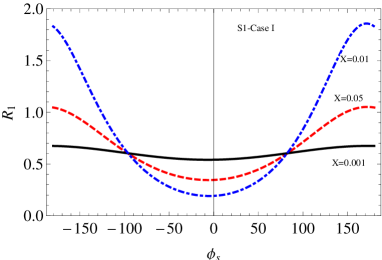
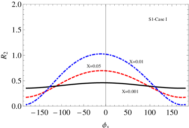
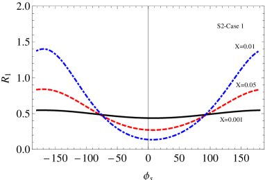
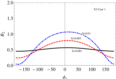
Figure 1: $R_{1}$ and $R_{2}$ as functions of weak phase $\phi_{s}$ with different $X$ in different scenarios and cases.

Finally, we will go back to the discussion of two scenarios. As aforementioned, $K_{0}^{*}(1430)$ is regarded as two-quark state in both S1 and S2, but the only controversy is whether it belongs to ground state or the first excited state. Through calculation and comparison above, we favor the second scenario, which means that $K_{0}^{*}(1430)$ is the lowest lying $\bar{q}q$ state. Namely, the scalar mesons lower than $1\mathbf{GeV}$ are four-quark states. This conclusion is also consistent with those of Refs.Cheng:2005nb ; shen ; Chen:2002si .

V Summary

Based on the QCD factorization approach, we have investigated in this work $B\to K_{0}^{*}\pi$ decays in the SM and a family non-universal $Z^{\prime}$ model. Because the inner structure of $K_{0}^{*}(1430)$ is not clear enough, we calculated the branching ratios under two different scenarios (S1 and S2). After calculation, we found that the branching ratios are sensitive to the weak annihilations. In the SM, with $\rho_{A}=1$ and $\phi_{A}\in[-30^{\circ},30^{\circ}]$, the branching ratios of S1 (S2) are smaller (larger) than the experimental data. Considering the $Z^{\prime}$ boson in two different cases, for S1, the branching ratios are still far away from experiment. For S2, the branching ratios become smaller and can accommodate the data in Case-II; in Case-I, the results can also explain the data but with large uncertainties. Furthermore, the other interesting observables, such as $CP$ asymmetries and isospin asymmetries, are also calculated. Compared with data, we favor that $K_{0}^{*}(1430)$ is the lowest lying $\bar{q}q$ state. Moreover, if there exists a $Z^{\prime}$ boson, Case-II is preferable. All above results will be tested in the B factories, LHC-b and the forthcoming super-B factory.

References

-
(1)
H. Y. Cheng and C. K. Chua,
Nucl. Phys. Proc. Suppl. 207-208, 391 (2010)
[arXiv:1012.5504 [hep-ph]];
A. J. Buras, arXiv:1106.0998 [hep-ph]. -
(2)
D. Asner et al. [Heavy Flavor Averaging Group],
arXiv:1010.1589 [hep-ex];
http://www.slac.stanford.edu/xorg/hfag. - (3) H. Y. Cheng, C. K. Chua and K. C. Yang, Phys. Rev. D 73, 014017 (2006) [arXiv:hep-ph/0508104].
-
(4)
M. Wirbel, B. Stech and M. Bauer,
Z. Phys. C 29, 637 (1985);
M. Bauer, B. Stech and M. Wirbel, Z. Phys. C 34, 103 (1987). -
(5)
A. Ali, G. Kramer, C. -D. Lu,
Phys. Rev. D58, 094009 (1998).
[hep-ph/9804363];
A. Ali, G. Kramer, C. -D. Lu, Phys. Rev. D59, 014005 (1999). [hep-ph/9805403];
H. -Y. Cheng and B. Tseng, Phys. Rev. D 58, 094005 (1998) [hep-ph/9803457]. -
(6)
Y. Y. Keum, H. N. Li and A. I. Sanda,
Phys. Rev. D 63, 054008 (2001)
[arXiv:hep-ph/0004173];
C. D. Lu, K. Ukai and M. Z. Yang, Phys. Rev. D 63, 074009 (2001) [arXiv:hep-ph/0004213]. -
(7)
M. Beneke, G. Buchalla, M. Neubert and C. T. Sachrajda,
Phys. Rev. Lett. 83, 1914 (1999)
[arXiv:hep-ph/9905312];
M. Beneke, G. Buchalla, M. Neubert and C. T. Sachrajda, Nucl. Phys. B 591, 313 (2000) [arXiv:hep-ph/0006124];
M. Beneke and M. Neubert, Nucl. Phys. B 675, 333 (2003) [arXiv:hep-ph/0308039]. -
(8)
C. W. Bauer, D. Pirjol and I. W. Stewart,
Phys. Rev. Lett. 87, 201806 (2001)
[arXiv:hep-ph/0107002];
C. W. Bauer, D. Pirjol and I. W. Stewart, Phys. Rev. D 65, 054022 (2002) [arXiv:hep-ph/0109045]. -
(9)
N. A. Tornqvist,
Phys. Rev. Lett. 49, 624 (1982);
G.L. Jaffe Phys. Rev. D 15, 267 (1977); Erratum-ibid. Phys. Rev. D 15 281 (1977);
A. L. Kataev, Phys. Atom. Nucl. 68, 567 (2005), Yad. Fiz. 68, 597(2005);
A. Vijande, A. Valcarce, F. Fernandez and B. Silvestre-Brac, Phys. Rev. D72, 034025 (2005). - (10) H. Y. Cheng and K. C. Yang, Phys. Rev. D 71, 054020 (2005) [arXiv:hep-ph/0501253].
- (11) H. Y. Cheng, C. K. Chua and K. C. Yang, Phys. Rev. D 77, 014034 (2008) [arXiv:0705.3079 [hep-ph]].
- (12) C. H. Chen, Phys. Rev. D 67, 014012 (2003) [arXiv:hep-ph/0210028].
- (13) C. H. Chen, C. Q. Geng, Y. K. Hsiao and Z. T. Wei, Phys. Rev. D 72, 054011 (2005) [arXiv:hep-ph/0507012].
- (14) W. Wang, Y. L. Shen, Y. Li and C. D. Lu, Phys. Rev. D 74, 114010 (2006) [arXiv:hep-ph/0609082].
- (15) Y. L. Shen, W. Wang, J. Zhu and C. D. Lu, Eur. Phys. J. C 50, 877 (2007) [arXiv:hep-ph/0610380];
-
(16)
C. s. Kim, Y. Li and W. Wang,
Phys. Rev. D 81, 074014 (2010)
[arXiv:0912.1718 [hep-ph]];
X. Liu, Z. Q. Zhang and Z. J. Xiao, Chin. Phys. C 34, 157 (2010) [arXiv:0904.1955 [hep-ph]];
X. Liu and Z. J. Xiao, Commun. Theor. Phys. 53, 540 (2010) [arXiv:1004.0749 [hep-ph]];
Z. Q. Zhang, Phys. Rev. D 82, 034036 (2010) [arXiv:1006.5772 [hep-ph]];
Z. Q. Zhang, Phys. Rev. D 82, 114016 (2010) [arXiv:1106.0103 [hep-ph]];
X. Liu, Z. J. Xiao and Z. T. Zou, arXiv:1105.5761 [hep-ph]. - (17) C. H. Chen and C. Q. Geng, Phys. Rev. D 75, 054010 (2007) [arXiv:hep-ph/0701023].
- (18) M. Cvetic and P. Langacker, Phys. Rev. D54, 3570 (1996) [arXiv:hep-ph/ 9511378].
- (19) R. W. Robinett and J. L. Rosner, Phys. Rev. D25, 3036 (1982) [Erratumibid. D 27, 679 (1983)].
- (20) N. Arkani-Hamed, A. G. Cohen and H. Georgi, Phys. Lett. B513, 232 (2001) [arXiv:hep-ph/0105239].
-
(21)
P. Fayet, Phys. Rev. D75, 115017 (2007)[arXiv:hep-ph/0702176];
C. H. Chen, C. Q. Geng and C. W. Kao, Phys. Lett. B663, 400 (2008) [arXiv:0708.0937 [hep-ph]]. - (22) P. Langacker and M. Plumacher, Phys. Rev. D 62, 013006 (2000) [arXiv:hep-ph/0001204].
-
(23)
V. Barger, et. al,
Phys. Lett. B 580, 186 (2004)
[arXiv:hep-ph/0310073];
V. Barger, et. al, Phys. Lett. B 598, 218 (2004) [arXiv:hep-ph/0406126];
V. Barger, et. al, arXiv:0906.3745 [hep-ph];
V. Barger, et. al, Phys. Rev. D 80, 055008 (2009) [arXiv:0902.4507 [hep-ph]]. -
(24)
K. Cheung, et. al,
Phys. Lett. B 652, 285 (2007)
[arXiv:hep-ph/0604223];
C. W. Chiang, et. al, JHEP 0608, 075 (2006) [arXiv:hep-ph/0606122]; -
(25)
Q. Chang, X. Q. Li and Y. D. Yang,
JHEP 0905, 056 (2009)
[arXiv:0903.0275 [hep-ph]];
Q. Chang, X. Q. Li and Y. D. Yang, JHEP 1002, 082 (2010) [arXiv:0907.4408 [hep-ph]];
Q. Chang, X. Q. Li and Y. D. Yang, JHEP 1004, 052 (2010) [arXiv:1002.2758 [hep-ph]];
Q. Chang and Y. H. Gao, Nucl. Phys. B 845, 179 (2011) [arXiv:1101.1272 [hep-ph]];
Y. Li, J. Hua and K. C. Yang, Eur. Phys. J. C 71, 1775 (2011) [arXiv:1107.0630 [hep-ph]];
J. Hua, C. S. Kim and Y. Li, Phys. Lett. B 690, 508 (2010) [arXiv:1002.2532 [hep-ph]];
J. Hua, C. S. Kim and Y. Li, Eur. Phys. J. C 69, 139 (2010) [arXiv:1002.2531 [hep-ph]]. - (26) P. Langacker, Rev. Mod. Phys. 81, 1199 (2009) [arXiv:0801.1345 [hep-ph]].
- (27) C. D. Lu, Y. M. Wang and H. Zou, Phys. Rev. D 75, 056001 (2007) [arXiv:hep-ph/0612210].
- (28) H.Y. Cheng, C.K. Chua, and C.W. Hwang, Phys. Rev. D 69, 074025 (2004).
-
(29)
G. Buchalla, A. J. Buras, and M. E. Lautenbacher, Rev. Mod. Phys. 68, 1125 (1996)
[hep-ph/9512380];
A. J. Buras, [hep-ph/9806471]. - (30) H.Y. Cheng, C.K. Chua, and A. Soni, Phys. Rev. D 71, 014030 (2005).